Integrated Operation of Multi-Reservoir and Many-Objective System Using Fuzzified Hedging Rule and Strength Pareto Evolutionary Optimization Algorithm (SPEA2)

Abstract

In this paper, a many-objective optimization algorithm was developed using SPEA2 for a system of four reservoirs in the Karun basin, including hydropower, municipal and industrial, agricultural, and environmental objectives. For this purpose, using 53 years of available data, hedging rules were developed in two modes: with and without applying fuzzy logic. SPEA2 was used to optimize hedging coefficients using the first 43 years of data and the last 10 years of data were used to test the optimized rule curves. The results were compared with those of non-hedging methods, including the standard operating procedures (SOP) and water evaluation and planning (WEAP) model. The results indicate that the combination of fuzzy logic and hedging rules in a many-objectives system is more efficient than the discrete hedging rule alone. For instance, the reliability of the hydropower requirement in the fuzzified discrete hedging method in a drought scenario was found to be 0.68, which is substantially higher than the 0.52 from the discrete hedging method. Moreover, reduction of the maximum monthly shortage is another advantage of this rule. Fuzzy logic reduced 118 million cubic meters (MCM) of deficit in the Karun-3 reservoir alone. Moreover, as expected, the non-hedging SOP and WEAP model produced higher reliabilities, lower average storages, and less water losses through spills.

1. Introduction

Iran is part of the arid and semi-arid regions of the world, with an average annual precipitation of about 250 mm, which is less than one-third of the world’s average annual rainfall. In such circumstances, optimum use of available water resources and the extracting optimize rule curve is important. The rule curve, as the main pattern of reservoir operation policy, determines the amount of water stored or released at each time step [1].

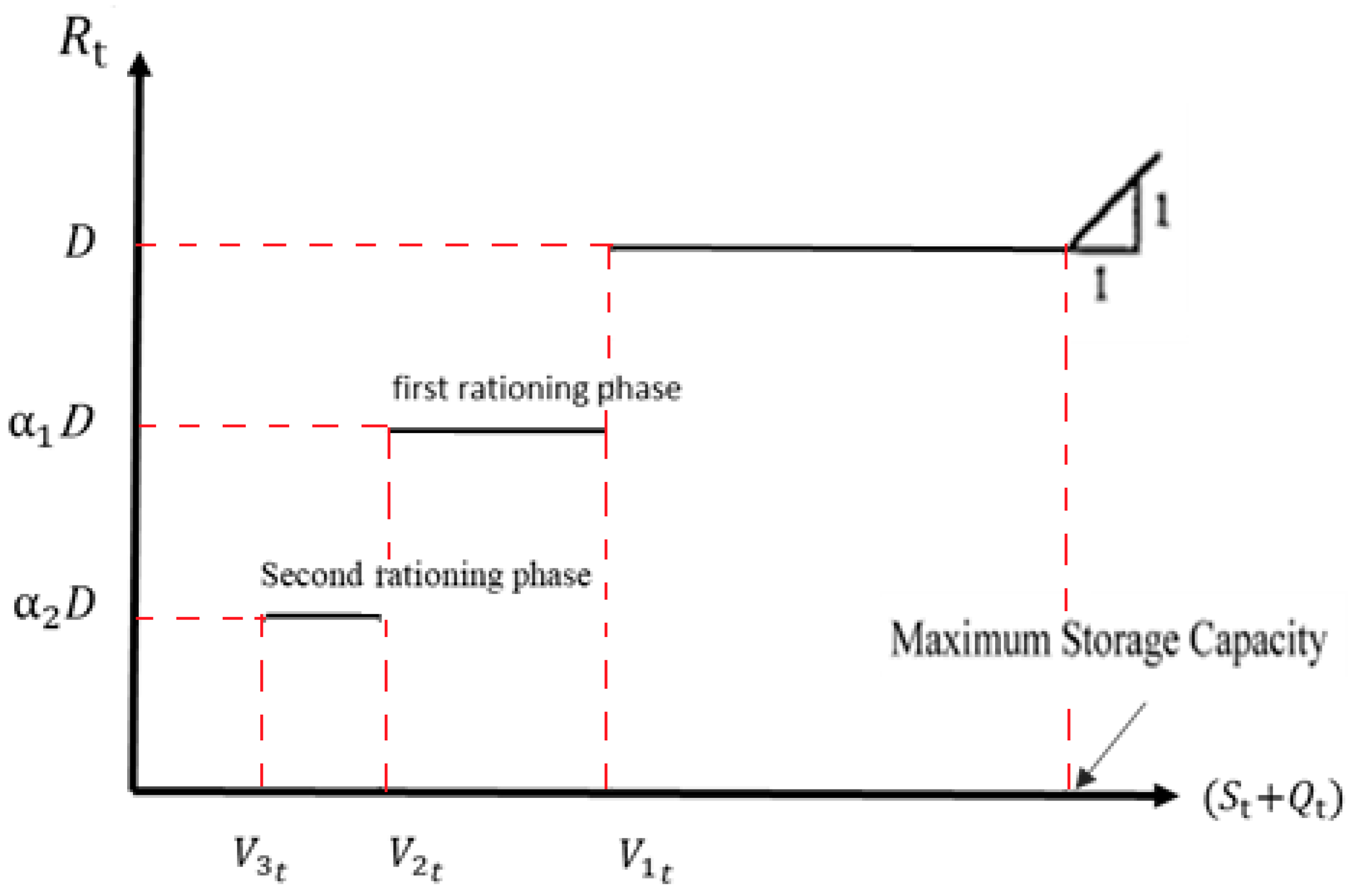
Applying hedging policies during drought periods can improve the utilization of water resources. This method is based on the fact that the higher number of drought periods with less intensity is preferred to fewer periods with higher intensity, mainly due to the nonlinear cost function of shortages. In other words, the relation between damages and deficiency is not linear [2]. The continuous hedging method was introduced in 1982 by Hashimoto et al. [3]. Later, Shih and ReVelle [4] introduced the discrete hedging method. In 1999, Neelakantan and Pundarikanthan improved the reservoir operation performance through the simulation–optimization procedure with the application of the hedging rule [5]. Considering the provision of hedging policies in recent years, many studies have been conducted to optimize utilization policies in drought periods, including the study by Dariane [2] to reduce the effect of drought. Dariane and Karami [6] presented an online optimization scheme for combined use of artificial neural networks (ANN), hedging policies, and the harmony search algorithm (HS) in developing optimum operating policies in a multiple-reservoir system. They developed a simulation–optimization methodology in which the management decision variables were passed from the optimization model to the simulation one to obtain the value of the objective function. Spiliotis et al. [7] presented a method by using the particle swarm optimization (PSO) algorithm for adopting the best hedging policy for reservoir operation. Jin et al. [8] reviewed the reservoir operation policies based on the discrete hedging method by using linear programming for the Hapcheon Reservoir in South Korea. In his research, hedging involved four phases, concern, caution, warning, and severe dehydration, in which the reservoir operation policies were determined based on the amount of available water and the tendency of the remaining reservoir in the existing phase. The amount of water in the reservoir also consisted of water stored at the beginning of the period plus the inflow into the reservoir.

In addition, in the past decades, a large number of papers have presented the fuzzy approach for improving the operation of reservoirs. For example, Russell and Campbell [9] used fuzzy logic programming to extract operational rules. Shrestha et al. [10] used a fuzzy rule-based model to derive operation rules for a multi-purpose reservoir. In this context, further research has been proposed using fuzzy logic theory to improve the efficiency in reservoir operation [11,12,13,14,15,16,17]. Ahmadinefar et al. [18,19] showed that the combination of hedging methods and fuzzy logic reduced the effects of drought because the rationing factors do not change suddenly when the combination is used. Rajendra et al. [20] and Kambalimath and Chandra Deka [21] reviewed fuzzy logic models for the operation of a single-purpose reservoir and hydrology and water resources domain, respectively.

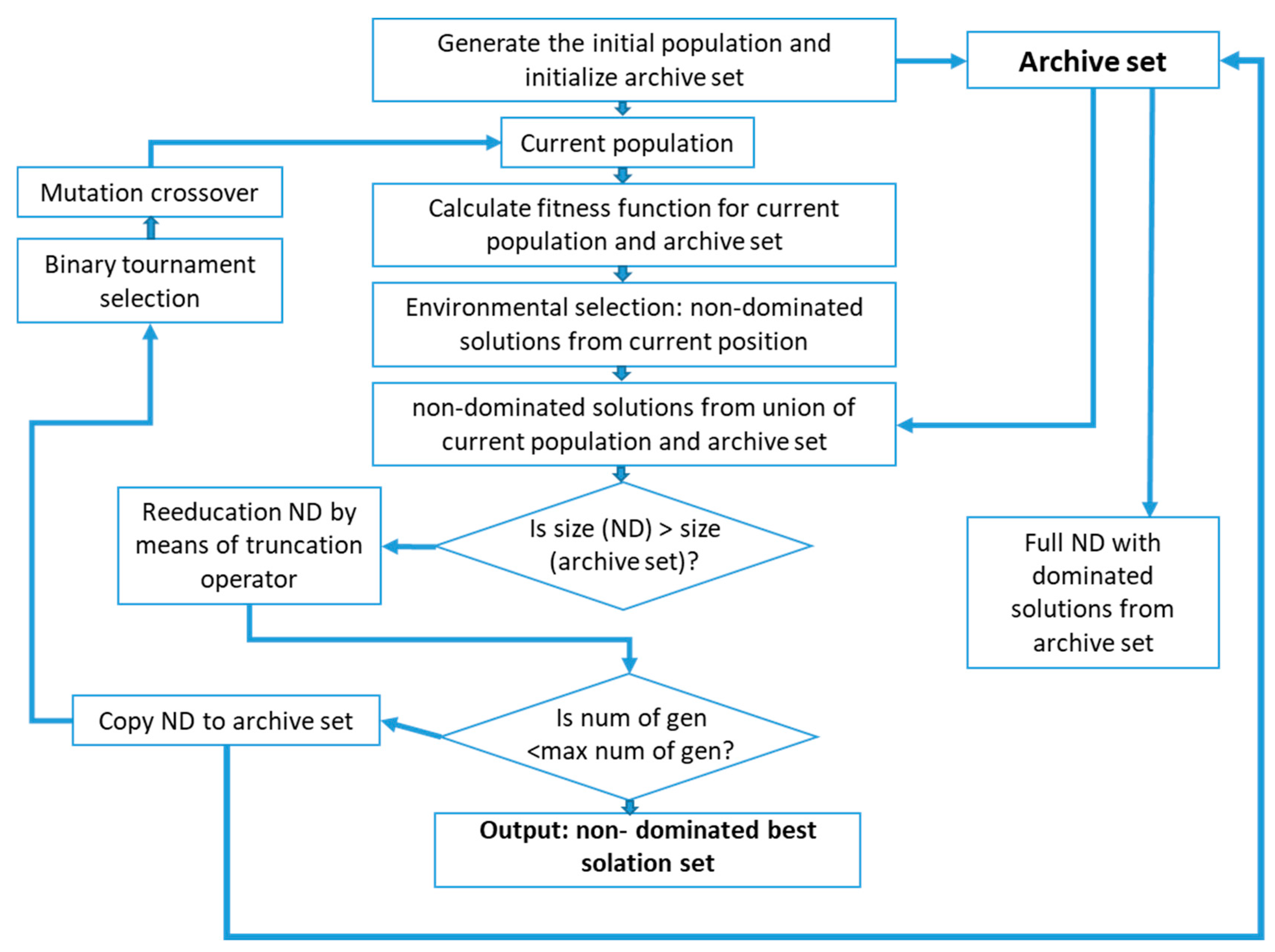
In discussing many-objective optimization algorithms (problems with more than three objective functions) visualization of a high-dimensional objective space and obtaining a good convergence of the Pareto front are challenges because the proportion of non-dominated objective solutions increases when the number of objectives exceeds four. This makes ranking difficult. Zitzler and Thiele [22] introduced the SPEA algorithm. This algorithm consists of a population set and an external set. The program begins with the initial population and the outer blanket, and the following operations are performed on each repetition. The dominant answers are copied to the empty set, and the evaluation function for all the existing answers is calculated. It is worth noting that the goal is to minimize the evaluation function. The SPEA2 method is the modified version of SPEA [23].

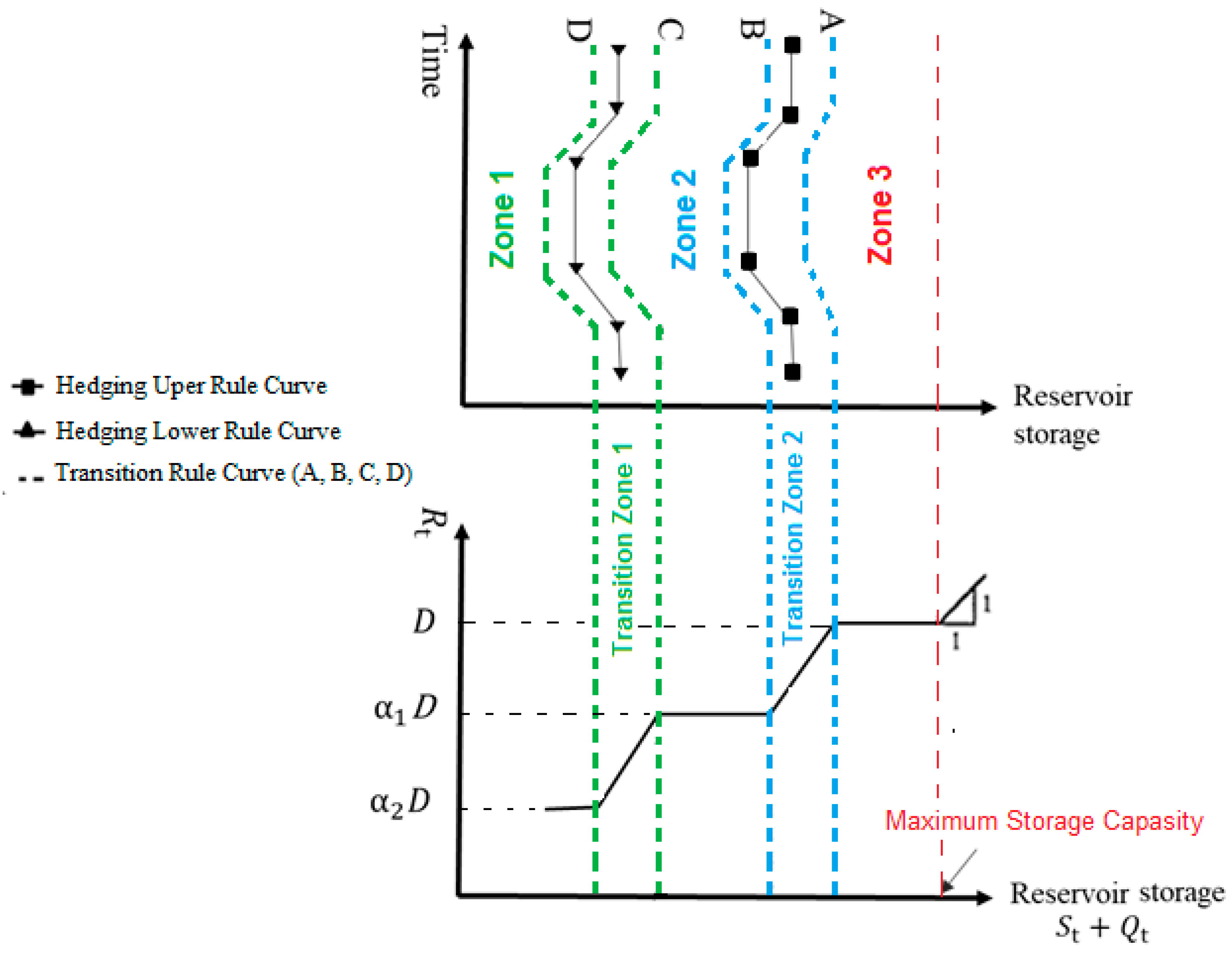
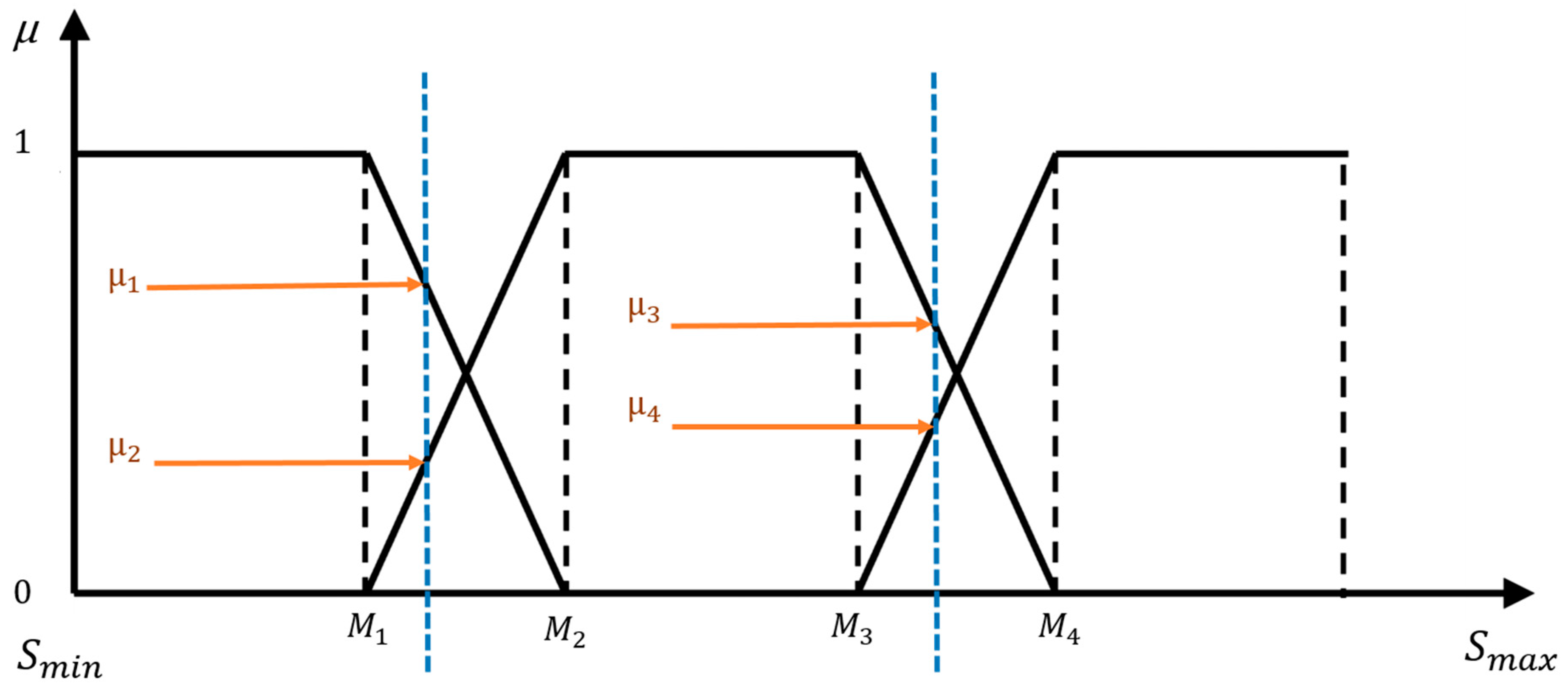
According to the importance of operating policies in drought periods, this study attempted to optimize the operation rules for a many-objective system (more than three objective functions), including the Karun-4, Karun-3, Karun-1, and Gotvand reservoirs, by using the hedging and fuzzy approach with the SPEA2 optimization algorithm. This study can help decision makers to decide how much water should be released now and how much should be retained for future uses, which is the major task of reservoir operation. This simple choice becomes complex in the presence of uncertain future inflows and nonlinear economic benefits for released water. Combining fuzzified hedging policies optimized with the SPEA2 optimization algorithm is a useful method in occurrence of severe and frequent droughts and can improve reservoir operation rules and aid water supply operators in coping with the risk of dramatic water deficiencies to the users. This is a new strategy for optimal operation of multiple reservoirs by combining discrete hedging and fuzzy theory during drought and water scarcity for a multi-reservoir, many-objective systems. It proposes water supply policies in the form of a rule curve and reduces drought effects in meeting demands. In the discrete hedging method, the hedging coefficient changes abruptly in each phase. Using the fuzzy approach creates a transition region for this coefficient and causes the coefficient to change gradually and mitigates the intensity of drought periods. In fact, the flexibility of the hedging factors increases by using fuzzy logic. Finally, vulnerability assessment, scarcity and reliability criteria are used to demonstrate the function of the fuzzy approach in hedging rules.

2. Methodology

2.1. Discrete Hedging Method

In this study, similar to Shih and ReVelle [4] and as shown in Figure 1, three hedging levels were assumed for the operation of reservoirs. In each reservoir, the amount of total available water (TAW), i.e., the sum of the initial reservoir storage, S_t, and the projected inflow, Q_t, in period t, was calculated during each time step. If TAW is above V_1t, then the normal condition is assumed, and all demands are fully met. In this case, the reservoir will spill if TAW increases to above the reservoir capacity plus demand. Hedging occurs when TAW falls under V_1t. If TAW is between V_1t and V_2t, the first water rationing phase is implemented where demand supply is cut down and only α₁ percent of the demand is released (0.4 ≤ α₁ ≤ 0.85). The second rationing phase is implemented if TAW falls further to a level between V_2t and V_3t, and α₂ percent of the demand is provided where 0.4 ≤ α₂ ≤ α₁ ≤ 0.85.

Therefore, decision variables for each reservoir examined in this study were: V_1t, V_2t, V_3t, α₁, and α₂. V_3t is equal to the minimum reservoir capacity (${\mathrm{S}}_{\min \mathrm{t}}$) according to the constraints of the problem, meaning no release occurs below this level. Hence, we must decide on four variables per month which is a total of 48 variables in a year. After determining the variables, the reservoir operation policy is applied in the following way:

$$\mathrm{If} {\mathrm{S}}_{\mathrm{ti}}+{\mathrm{Q}}_{\mathrm{ti}}< \mathrm{V}{3}_{\mathrm{t}} \mathrm{Then} {\mathrm{R}}_{\mathrm{ti}}=0$$

(1)

$$\mathrm{Else} \mathrm{If} {\mathrm{V}}_{3\mathrm{ti}} < {\mathrm{S}}_{\mathrm{ti}}+{\mathrm{Q}}_{\mathrm{ti}}< {\mathrm{V}}_{2\mathrm{ti}} \mathrm{Then} {\mathrm{R}}_{\mathrm{ti}}=\mathsf{\alpha }{2}_{\mathrm{ti}} * {\mathrm{D}}_{\mathrm{ti}}$$

(2)

$$\mathrm{Else} \mathrm{If} {\mathrm{V}}_{2\mathrm{ti}} < {\mathrm{S}}_{\mathrm{ti}}+{\mathrm{Q}}_{\mathrm{ti}}< {\mathrm{V}}_{1\mathrm{ti}} \mathrm{Then} {\mathrm{R}}_{\mathrm{ti}}=\mathsf{\alpha }{1}_{\mathrm{ti}} * {\mathrm{D}}_{\mathrm{ti}}$$

(3)

$$\mathrm{Else} \mathrm{If} {\mathrm{V}}_{1\mathrm{ti}} < {\mathrm{S}}_{\mathrm{ti}}+{\mathrm{Q}}_{\mathrm{ti}} \mathrm{Then} {\mathrm{R}}_{\mathrm{ti}}={\mathrm{D}}_{\mathrm{ti}}$$

(4)

$$\begin{array}{c}\mathrm{Else} \mathrm{if} {\mathrm{S}}_{\max \mathrm{i}}> {\mathrm{S}}_{\mathrm{ti}}+{\mathrm{Q}}_{\mathrm{ti}} \mathrm{Then} {\mathrm{R}}_{\mathrm{ti}}={\mathrm{D}}_{\mathrm{ti}} \mathrm{and} {\mathrm{Spill}}_{\mathrm{ti}}+{\mathrm{Q}}_{\mathrm{ti}}={\mathrm{S}}_{\mathrm{ti}}+{\mathrm{Q}}_{\mathrm{ti}}-\\ {\mathrm{S}}_{\max \mathrm{i}}\end{array}$$

(5)

where R_ti, D_ti, S_ti, Q_ti, Spill_ti is the release, demand, storage, inflow, and spill of reservoir i in period t. S_{min t} and S_{max t} are the minimum and maximum capacity of the reservoir i. If the constraints of the problem are violated, a penalty is considered for R_ti in order to remove that choice from the optimization process and make it feasible.

2.2. Fuzzified Discrete Hedging Method

Fuzzy logic was first introduced by Zadeh in 1973. In fuzzy logic, the membership function specifies how each point is mapped to a membership value between 0 and 1 [24,25]. If the membership grade of an element is 0, then that member is completely out of the set, and if it is equal to 1, that member is completely in the set. Now, if it is between 0 and 1, this number represents the degree of gradual membership. In this research, the trapezoidal membership function was used to apply fuzzy logic. In the discrete hedging method, the hedging coefficient changes suddenly in each phase. Using the fuzzy approach creates a transition region for this coefficient and causes the coefficient to change gradually. The schematic diagram (Figure 2) shows the fuzzy hedging rule.

In Figure 2, there are two line curves (upper and lower curves) and four transition paths. When the available water is in zone 2 (between transmission lines B and C), α₁ percent of demand is provided. If the available water is higher than the transmission line B, the coefficient is determined between α₁ and 1 by using the fuzzy membership function. It is the first phase of hedging for slight droughts. The same trend is considered for the second phase for severe droughts. When the available water is below the transmission line C, the coefficient is determined between α₂ and α₁ by using the fuzzy membership function. Using transition zones around the rule curves in fuzzy logic prevents the sudden change of coefficients. In the other words, where the reservoir level is going from one zone to another, the hedging coefficients will be increased or decreased gradually. Trapezoidal membership function is shown in Figure 3.

The operation policy of each reservoir is defined by Equations (6)–(15). μ is the degree of belongingness to a fuzzy set and Equations (6)–(9) present the parameters of determining the trapezoidal membership function. The main approach for the developed hedging rule is illustrated in Equations (10)–(15).

$${\mathrm{M}}_{1\mathrm{ti}}={\mathrm{S}}_{\min \mathrm{i}}+({\mathrm{V}}_{2\mathrm{ti}} -{ \mathrm{S}}_{\min \mathrm{i}}) * {\mathsf{\beta }}_{1\mathrm{ti}}$$

(6)

$${\mathrm{M}}_{2\mathrm{ti}}={\mathrm{V}}_{2\mathrm{ti}}+({\mathrm{V}}_{1\mathrm{ti}} - {\mathrm{V}}_{2\mathrm{ti}}) * {\mathsf{\beta }}_{2\mathrm{ti}}$$

(7)

$${\mathrm{M}}_{3\mathrm{ti}}={\mathrm{M}}_2+({\mathrm{V}}_{1\mathrm{ti}} - {\mathrm{M}}_{2\mathrm{ti}}) * {\mathsf{\beta }}_{3\mathrm{ti}}$$

(8)

$${\mathrm{M}}_{4\mathrm{ti}}={\mathrm{V}}_{1\mathrm{ti}}+({\mathrm{S}}_{\max \mathrm{i} }-{ \mathrm{V}}_{1\mathrm{ti}}) * {\mathsf{\beta }}_{4\mathrm{ti}}$$

(9)

$$\mathrm{If} {\mathrm{S}}_{\mathrm{ti}}+{\mathrm{Q}}_{\mathrm{ti}} Є \mathrm{zone} 3 \mathrm{Then} {\mathrm{R}}_{\mathrm{ti}}={\mathrm{D}}_{\mathrm{ti}}$$

(10)

$$\mathrm{If} {\mathrm{S}}_{\mathrm{ti}}+{\mathrm{Q}}_{\mathrm{ti}} Є \mathrm{transition} \mathrm{zone} 2 \mathrm{Then} {\mathrm{R}}_{\mathrm{ti}}=( {\mu }_3{\mathsf{\alpha }}_{1\mathrm{ti}}+{\mu }_4) * {\mathrm{D}}_{\mathrm{ti}}$$

(11)

$$\mathrm{If} {\mathrm{S}}_{\mathrm{ti}}+{\mathrm{Q}}_{\mathrm{ti}} Є \mathrm{zone} 2 \mathrm{Then} {\mathrm{R}}_{\mathrm{ti}}={\mathsf{\alpha }}_{1\mathrm{ti}} * {\mathrm{D}}_{\mathrm{ti}}$$

(12)

$$\mathrm{If} {\mathrm{S}}_{\mathrm{ti}}+{\mathrm{Q}}_{\mathrm{ti}} Є \mathrm{transition} \mathrm{zone} 1 \mathrm{Then} {\mathrm{R}}_{\mathrm{ti}}=( {\mu }_1{\mathsf{\alpha }}_{2\mathrm{ti}}+{\mu }_2{\mathsf{\alpha }}_{1\mathrm{ti}}) * {\mathrm{D}}_{\mathrm{ti}}$$

(13)

$$\mathrm{If} {\mathrm{S}}_{\mathrm{ti}}+{\mathrm{Q}}_{\mathrm{ti}} Є \mathrm{zone} 1 \mathrm{Then} {\mathrm{R}}_{\mathrm{ti}}={\mathsf{\alpha }}_{1\mathrm{ti}} * {\mathrm{D}}_{\mathrm{ti}}$$

(14)

$$\mathrm{If} {\mathrm{S}}_{\mathrm{ti}}+{\mathrm{Q}}_{\mathrm{ti}} < \mathrm{V}{3}_{\mathrm{ti}} \mathrm{Then} {\mathrm{R}}_{\mathrm{ti}}=0$$

(15)

S, Q, V, R, D, and α were defined before in Section 2.1. β_1ti, β_2ti, β_3ti, and β_4ti are the membership function parameters and are obtained by applying optimization algorithm. Hence, based on this method, with V_1t, V_2t, α₁, and α₂, there are eight decision variables for optimization in each time period.

2.3. SPEA2 Optimization Algorithm

The SPEA algorithm consists of a population set and an external set [22]. The program begins with the initial population and the blank outer set, and the following operations are performed on each repetition. The dominant answers are copied to the empty external set, and the evaluation function for all the existing answers is calculated as follows (Figure 4). It is worth noting that the goal is to minimize the evaluation function. For each solution (i) in the external, S(i) is assigned between 0 and 1. This is the ratio of solutions that are dominated by i to the population size plus 1 and represents the evaluation function of that answer. For the solutions (j) in the population set, the evaluation function is obtained from the sum of S(i) for solutions dominant j plus 1. Finally, depending on the evaluation function, the mating, combination and mutation operators are performed, and the new set replaces the previous one.

The SPEA2 method is the modified version of SPEA. In this algorithm, S(i) and R(i) are computed as follows. ${\mathrm{P}}_{\mathrm{t}}$ and $\overline{{\mathrm{P}}_{\mathrm{t}}}$ in are population and external sets, respectively. In the following equations, the ≺ symbol indicates that solution i is dominant j [23].

$$\mathrm{S}\left(\mathrm{i}\right)=\left|\left\{\mathrm{j}| \mathrm{j} \mathsf{ϵ}{ \mathrm{P}}_{\mathrm{t}}+\overline{{\mathrm{P}}_{\mathrm{t}}} ^\mathrm{i} > \mathrm{j} \right\}\right|$$

(16)

$$\mathrm{R}(\mathrm{i})={{\displaystyle \sum }}_{{\mathrm{P}}_{\mathrm{t}}+\overline{{\mathrm{P}}_{\mathrm{t}}} , \mathrm{J}>\mathrm{i}}\mathrm{S}\left(\mathrm{j}\right)$$

(17)

To calculate the evaluation function of each solution, the D(i) parameter, which also contains the distance information from the nearest neighbor, k, is added to R(i). For this purpose, the distance between the solution i and all solutions in the population and the external set j is calculated and incrementally arranged in a list. The solution k is represented by ${\mathsf{\sigma }}_{\mathrm{i}}^{\mathrm{k}}$, where k is the root of total number of solutions in population and external sets. Finally, D(i) and the evaluation function F(i) are calculated as follows.

$$\mathrm{D}(\mathrm{i})=\frac{1}{{\mathsf{\sigma }}_{\mathrm{i}}^{\mathrm{k}}+2}$$

(18)

F(i) = R(i) + D(i)

(19)

In this research, the number of iterations was considered as 3000.

2.4. Water Evaluation and Planning (WEAP)

WEAP is a software tool that was developed for integrated water resources simulation. It can cover a wide range of issues, such as water protection, rights and allocation priorities, simulation of surface water and groundwater, reservoir operation, hydropower generation, pollution control, ecosystem demands, vulnerability assessment, and benefit–cost analysis of the project [26].

Water allocation in this program is based on priorities that can range from 1 to 99. Reservoirs are also considered as a demand site with a priority of 99 so they will fill only when there is additional water in the system. The objective function is maxmization of the coverage rate for all demand sites. WEAP uses linear programming and iterates for each priority so that demands with priority 1 are supplied first and before priority 2. Hence, the program is run at least once for each priority. If one demand site can be able to supply its water from several sources, the resources are also prioritized. The WEAP simulation model is able to optimize allocations among different users in each time step. It is not capable of maximizing throughout the time and has no hedging mechanism by itself, and thus acts similar to the standard operating procedures (SOP) method in this regard. Here, the output of this model was mainly used as a base solution for comparison purposes.

3. Case Study

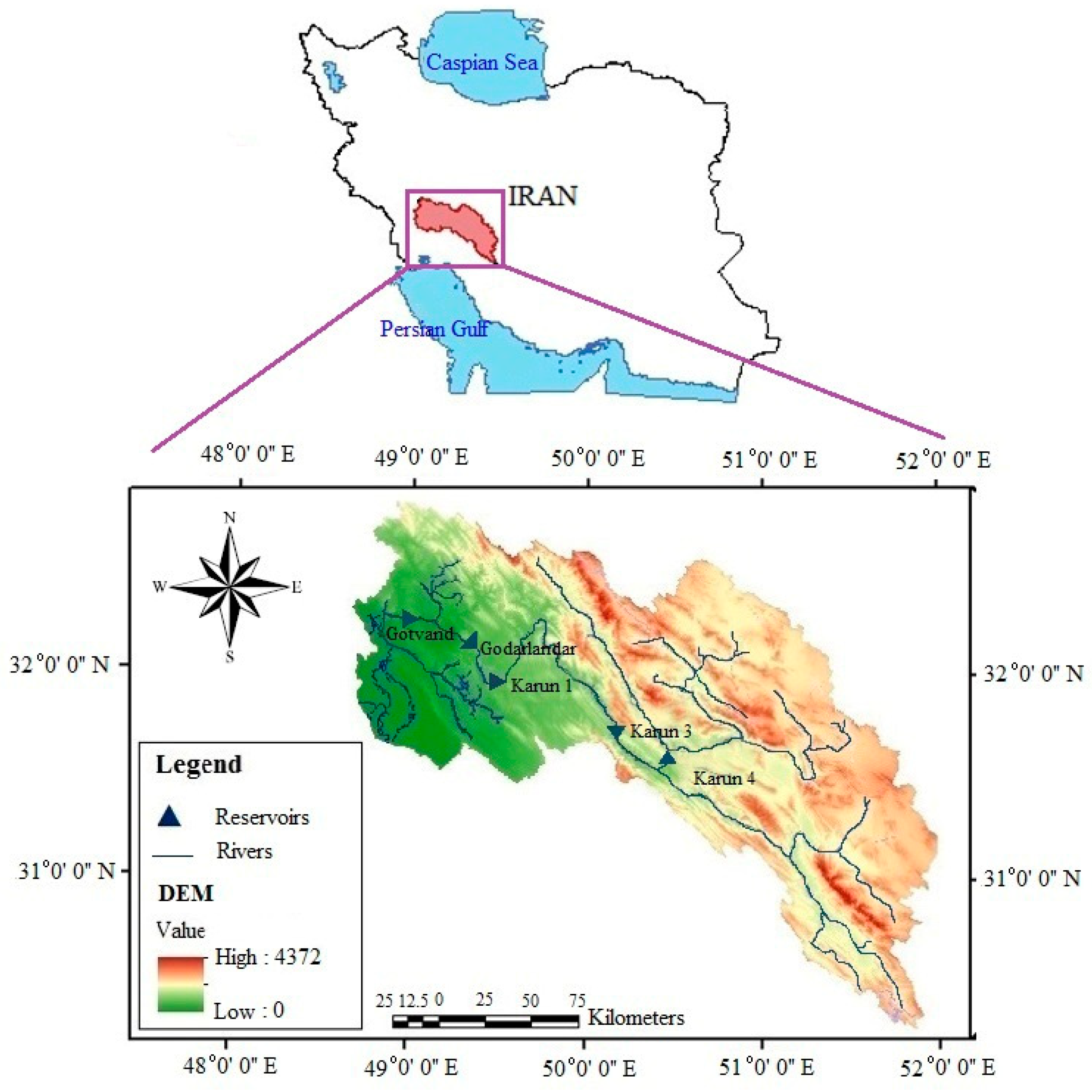
The study area was the Karun basin in southwestern Iran. Five reservoirs, including the Karun-4, Karun-3, Karun-1, Godarlandar, and Gotvand reservoirs, along with their demand site were used in this paper to evaluate the methods (Figure 5). It should be noted that the Godarlandar reservoir does not play a role in downstream flow regulations; therefore, it was removed from the optimization process, leaving a system of four reservoirs.

The whole Karun basin area is about 67,100 km², where 68% is in the mountains and 32% is in the plains. Karun River, with a length of 950 km, is the longest river in the country and one of the longest in the Middle East. The river originates from the Zagros Mountains and drains into Persian Gulf after passing the Khuzestan Plain. The river is also considered the largest river in Iran in terms of annual discharge [27].

The schematic of the study area is shown in Figure 6.

Data and System Specifications

The time series studied in this paper were monthly data during the 1961–1962 to 2013–2014 water years, from which the initial 43 years were considered for optimization of decision parameters and the last 10 years were used for testing the performance of the optimized rule curves.

Table 1. Specifications of reservoirs and power plants.

Parameter	Karun-4	Karun-3	Karun-1	Gotvand
Normal water level, masl *	1028	845	532.5	372
Top of active storage, masl	996	800	490	185
Total reservoir capacity, MCM	2279	2718	2438	4671
Active storage, MCM	834.2	1624.5	1614	3050.5
Hydropower plant capacity, MW **	1000	2000	2000	2000
Number of HP units	4	8	8	8
Design discharge, cms +	684	1370.5	1471	1686.3
Design head, m ++	162	161	154	130
HP efficiency, %	92	92.4	90	93
Peak power duration, h ~	4	4	4	6
Average head loss, m	3	4.5	8	4

* meters above sea level, ** megawatts, ⁺ cubic meters per second, ⁺⁺ meters, ^~ hours.

shows a summary of the reservoir information.

The priority of demands for the Karun-4, Karun-3, and Karun-1 reservoirs is as follows: 1-hydropower, 2-municipal, 3-environmental, and 4-agricultural demands. In the Gotvand reservoir, energy production is the secondary objective after all others. Therefore, due to high agricultural and municipal demands and in order to increase the reservoir efficiency for the secondary demand (hydropower), two outlets were devised. The height of the penstock (for releasing water for hydropower generation) is 181 masl and the height of the reservoir lower outlet for other uses (e.g., agriculture, municipal, etc.) is 161 masl. All other demands are released through the penstock for energy generation as long as possible. In dry periods, where the storage level falls below the penstock level (i.e., 181 m), the demand is released through the lower outlet of the reservoir.

Table 2. Municipal and agricultural demands (MCM).

Sector	Karun-4	Karun-3	Karun-1	Gotvand
Municipal	0.4	9.8	0.8	116.2
Agricultural	1.3	0.4	8.6	497.2

shows the monthly average municipal and agricultural demands in each reservoir site.

The returned water from agricultural fields is not usually estimated accurately and there is no report regarding this parameter in the area. Hence, in the present study, the rate of return flow was considered as 20% of the diverted flow. Moreover, according to the recommendation of Tennant [28], the monthly minimum streamflow for environmental concerns at the downstream of each reservoir was assumed as the 10% of average monthly natural streamflow.

To calculate the reservoir’s hydropower requirement, following parameters are needed:

(1)

Hydropower plant capacity (MW), design head (m), and head loss (m), which can be expressed as a constant or a function of other parameters.

(2)

Number of units of power plants and the peak hours, which can be different for each month.

(3)

Efficiency (%), flood level (m of sea level), and design discharge rate (cms).

(4)

Moreover, the net head (m), the required discharge rate for firm energy production (cms), and the hydropower demand are obtained from Equations (20)–(22).

$${\mathrm{H}}_{\mathrm{net},\mathrm{t}}=\frac{{\mathrm{H}}_{\mathrm{t}}+{\mathrm{H}}_{\mathrm{t}+1}}{2}-\mathrm{TWL}-\mathrm{HL}$$

(20)

$${\mathrm{Q}}_{\mathrm{req},\mathrm{t}}=(\frac{\mathrm{P} \ast 1000}{9.81{ \ast \mathsf{\eta } \ast \mathrm{H}}_{\mathrm{net},\mathrm{t}}})$$

(21)

$${\mathrm{D}}_{\mathrm{t}} ={\mathrm{Q}}_{\mathrm{req},\mathrm{t}}\ast \mathrm{PT}\ast \mathrm{Nday} \ast 3600/{10}^6$$

(22)

where H_t, TWL, HL, H_net,t, P, η, D_t, PT, and Nday are the reservoir level at the beginning of period t (masl), tail water level (masl), head loss (m), net head (m), power plant installation capacity (MW), plant efficiency (%), required water for hydropower demand (MCM), and daily peak hours and number of days in a month, respectively.

4. Applications

In this study the objective functions were the minimization of the normalized deficits for each demand as described by Equations (23)–(26).

$${ \mathrm{Min} \mathrm{TSD}}_{\mathrm{mun}}={\sum }_{\mathrm{i}=1}^4{\sum }_{\mathrm{t}=1}^{\mathrm{T}}{(\frac{{\mathrm{D}}_{\mathrm{tmun} \mathrm{i}}-{\mathrm{R}}_{\mathrm{tmun} \mathrm{i}}}{{\mathrm{D}}_{\mathrm{tmun} \mathrm{i}}})}^2 \mathrm{Municipal}$$

(23)

$${\mathrm{Min} \mathrm{TSD}}_{\mathrm{agr}}={\sum }_{\mathrm{i}=1}^4{\sum }_{\mathrm{t}=1}^{\mathrm{T}}{(\frac{{\mathrm{D}}_{\mathrm{tagr} \mathrm{i}}-{\mathrm{R}}_{\mathrm{tagr} \mathrm{i}}}{{\mathrm{D}}_{\mathrm{tagr} \mathrm{i}}})}^2 \mathrm{Agriculture}$$

(24)

$${\mathrm{Min} \mathrm{TSD}}_{\mathrm{env}}={\sum }_{\mathrm{i}=1}^4{\sum }_{\mathrm{t}=1}^{\mathrm{T}}{(\frac{{\mathrm{D}}_{\mathrm{tenv} \mathrm{i}}-{\mathrm{R}}_{\mathrm{tenv} \mathrm{i}}}{{\mathrm{D}}_{\mathrm{tenv} \mathrm{i}}})}^2 \mathrm{Environmental}$$

(25)

$${\mathrm{Min} \mathrm{TSD}}_{\mathrm{hyd}}={\sum }_{\mathrm{i}=1}^4{\sum }_{\mathrm{t}=1}^{\mathrm{T}}{(\frac{{\mathrm{D}}_{\mathrm{thyd} \mathrm{i}}-{\mathrm{R}}_{\mathrm{thyd} \mathrm{i}}}{{\mathrm{D}}_{\mathrm{thyd} \mathrm{i}}})}^2 \mathrm{Hydropower}$$

(26)

In the above equations, the index i represents the reservoir number (1 to 4), R_ti and D_ti are the reservoir release and demand, respectively.

Constraints and assumptions of the problem are given as follows.

$${\mathrm{S}}_{\mathrm{t}+1 \mathrm{i}}={\mathrm{S}}_{\mathrm{ti}}+{\mathrm{Q}}_{\mathrm{ti}}-{\mathrm{R}}_{\mathrm{ti}}-{\mathrm{Spill}}_{\mathrm{ti}}-{\mathrm{E}}_{\mathrm{ti}} \mathrm{mass} \mathrm{balance}$$

(27)

$${\mathrm{S}}_{\min \mathrm{i}}< {\mathrm{S}}_{\mathrm{ti}} < {\mathrm{S}}_{\max \mathrm{i}}\mathrm{capacity} \mathrm{constraint}$$

(28)

$$0.4 < {\mathsf{\alpha }}_{2\mathrm{i}}< {\mathsf{\alpha }}_{1\mathrm{i}} < 0.85 \mathrm{assumptions} \mathrm{of} \mathrm{hedging}$$

(29)

$${\mathrm{S}}_{\min \mathrm{i}}< {\mathrm{V}}_{2\mathrm{i}} < {\mathrm{V}}_{1\mathrm{i}} < {\mathrm{S}}_{\max \mathrm{i}} \mathrm{assumptions} \mathrm{of} \mathrm{hedging}$$

(30)

$${\mathrm{S}}_{1\mathrm{i}}=0.9 * {\mathrm{S}}_{\max \mathrm{i}} \mathrm{initial} \mathrm{storage}$$

(31)

$$\mathrm{If} {\mathrm{R}}_{\mathrm{thyd} \mathrm{i}}>{\mathrm{R}}_{\mathrm{tmun} \mathrm{i}}+{\mathrm{R}}_{\mathrm{tagr} \mathrm{i}}+{\mathrm{R}}_{\mathrm{tenv} \mathrm{i}}=> \mathrm{extra}={\mathrm{R}}_{\mathrm{thyd} \mathrm{i}}- ({\mathrm{R}}_{\mathrm{tmun} \mathrm{i}}+{\mathrm{R}}_{\mathrm{tenv} \mathrm{i}})$$

(32)

$$\begin{array}{c}{\mathrm{Q}\prime }_{\mathrm{ti}+1}={\mathrm{Q}}_{\mathrm{ti}+1}-0.9 * {\mathrm{Q}}_{\mathrm{ti}}+{\mathrm{Spill}}_{\mathrm{ti}}+0.2 * {\mathrm{R}}_{\mathrm{tagr} \mathrm{i}}+{\mathrm{R}}_{\mathrm{tenv} \mathrm{i}}+\mathrm{extra} \mathrm{The}\\ \mathrm{relationship} \mathrm{between} \mathrm{each}\mathrm{upstream} \mathrm{and} \mathrm{the} \mathrm{next} \mathrm{downstream} \mathrm{reservoirs}\end{array}$$

(33)

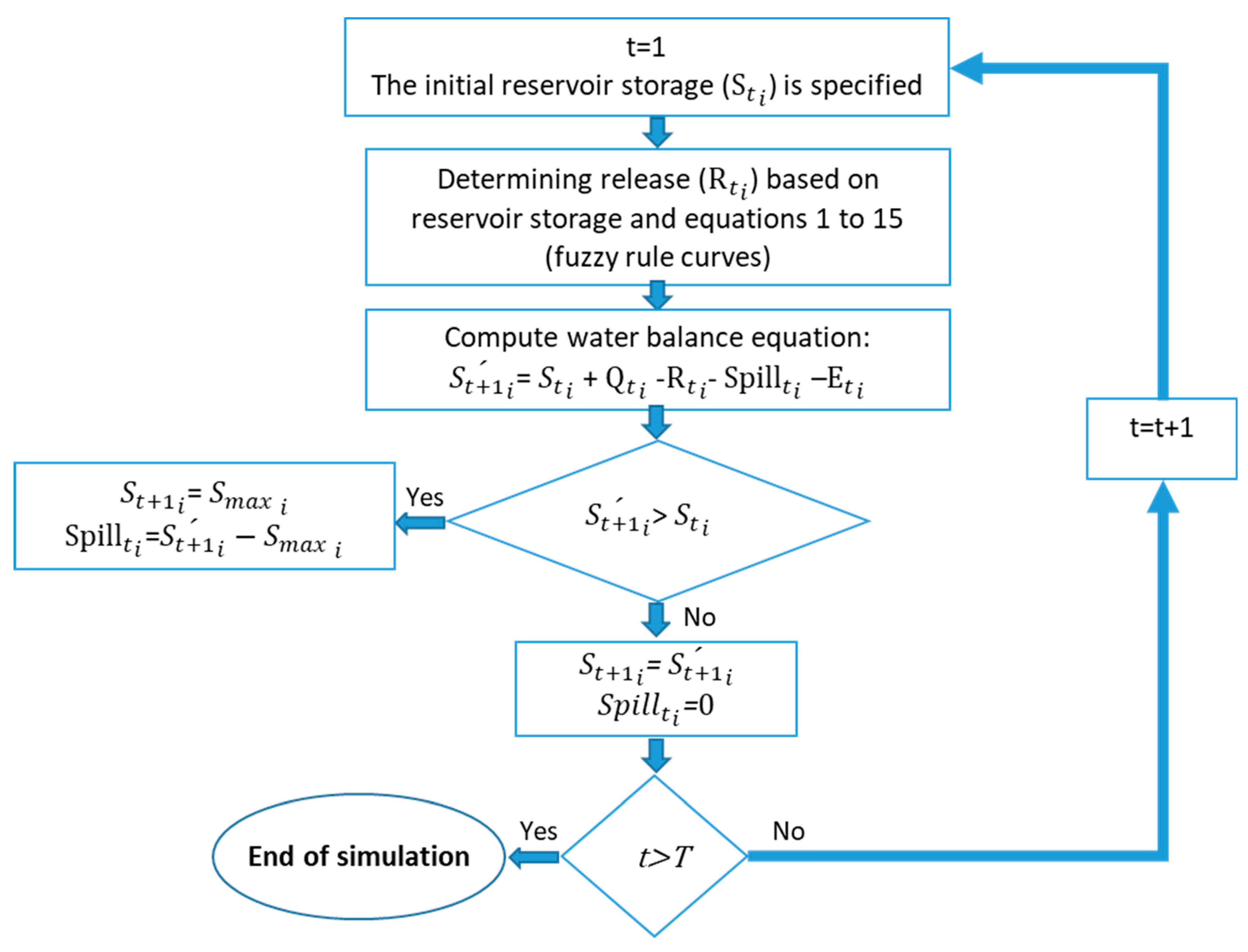
The simulation method for a fuzzified discrete hedging approach is presented in Figure 7. The steps are as follows:

1.

For the first month (t = 1), the initial reservoir storage (${\mathrm{S}}_1{}_{\mathrm{i}}$) is equal to ${\mathrm{S}}_{\mathrm{m}\mathrm{a}\mathrm{x} }{}_i$ and ${\mathrm{Spill}}_1{}_i=$ 0.

2.

The releases (${\mathrm{R}}_t{}_i$) are obtained in each period according to the rule curve based on optimized coefficients (according to Equations (1)–(5) for discrete hedging and 10 to 15 for the fuzzified discrete hedging method).

3.

The mass balance equation (Equation (27)) is calculated, and spill and reservoir storage are determined in the next month.

4.

The above steps are repeated until the last month of the time series.

In this study, 53 years of measured data were available from which 43 years of data were used for the optimization phase and the last 10 years were applied for testing the performance of optimized rule curves.

5. Results

5.1. Calibration Stage

In this section, the results of the fuzzified discrete hedging rule are compared with the discrete hedging rule, the SOP method, and the WEAP model. The convergence graph of the fuzzified discrete hedging rule is illustrated in Figure 8. According to this figure, the SPEA2 optimization algorithm had almost the same trend for all four objective functions. The agricultural and municipal functions had the most and the least convergence rates, respectively.

Table 3. Discrete hedging and fuzzified discrete hedging coefficients.

Method	Reservoir	Coef.	Mar	Apr	May	June	July	Aug	Sep	Oct	Nov	Dec	Jan	Feb	Avg
Fuzzified Discrete Hedging	Karun-4	${\mathrm{V}}_{1\mathrm{P}}$	2052	2085	1962	1951	1963	2028	1905	2101	2001	1463	1839	1861	1934
	Karun-3	${\mathrm{V}}_{1\mathrm{P}}$	1298	1352	1895	2061	2392	1647	1209	1654	1990	1984	1769	1758	1751
	Karun-1	${\mathrm{V}}_{1\mathrm{P}}$	1754	2041	2130	1633	1997	1505	2438	2409	1620	1883	2285	1246	1912
	Gotvand	${\mathrm{V}}_{1\mathrm{P}}$	3738	2833	1913	2677	3401	3059	3586	4668	4320	3327	2870	2794	3266
	Karun-4	${\mathrm{V}}_{2\mathrm{P}}$	1841	1504	1445	2001	1514	1480	1646	1881	1719	1641	1445	1742	1655
	Karun-3	${\mathrm{V}}_{2\mathrm{P}}$	1094	1306	1094	1202	1094	1510	1094	1459	1094	1414	1292	1190	1237
	Karun-1	${\mathrm{V}}_{2\mathrm{P}}$	1510	934	824	1068	1741	1471	2240	2067	824	1678	2142	824	1443
	Gotvand	${\mathrm{V}}_{2\mathrm{P}}$	1976	1710	1710	2450	2662	2562	3452	3208	1710	3224	1710	1710	2340
	Karun-4	α1	0.71	0.84	0.85	0.76	0.72	0.73	0.76	0.74	0.85	0.85	0.6	0.59	0.75
	Karun-3	α1	0.64	0.61	0.85	0.85	0.76	0.6	0.81	0.85	0.84	0.85	0.6	0.57	0.73
	Karun-1	α1	0.82	0.83	0.65	0.83	0.7	0.84	0.85	0.6	0.57	0.65	0.84	0.85	0.75
	Gotvand	α1	0.79	0.75	0.7	0.85	0.64	0.73	0.67	0.63	0.81	0.52	0.85	0.76	0.72
	Karun-4	α2	0.54	0.62	0.69	0.73	0.65	0.58	0.53	0.61	0.59	0.77	0.58	0.4	0.61
	Karun-3	α2	0.59	0.49	0.81	0.4	0.66	0.57	0.77	0.59	0.4	0.72	0.59	0.4	0.58
	Karun-1	α2	0.43	0.78	0.5	0.57	0.67	0.66	0.62	0.58	0.4	0.54	0.68	0.57	0.58
	Gotvand	α2	0.47	0.68	0.59	0.41	0.58	0.42	0.46	0.63	0.7	0.44	0.46	0.61	0.54
Discrete-Hedging	Karun-4	${\mathrm{V}}_{1\mathrm{P}}$	1895	2019	2181	1646	2000	1838	1863	2030	1902	2232	2007	1875	1957
	Karun-3	${\mathrm{V}}_{1\mathrm{P}}$	1794	1973	1367	2106	1984	1159	1781	2330	2718	2215	2141	2108	1973
	Karun-1	${\mathrm{V}}_{1\mathrm{P}}$	1815	1987	1210	1519	1688	1137	2438	1803	1595	1919	1837	1425	1698
	Gotvand	${\mathrm{V}}_{1\mathrm{P}}$	3513	2764	3440	3912	2571	3425	3109	3925	3423	3759	3002	4071	3400
	Karun-4	${\mathrm{V}}_{2\mathrm{P}}$	1648	1837	1984	1536	1774	1757	1753	1817	1525	1719	1513	1844	1726
	Karun-3	${\mathrm{V}}_{2\mathrm{P}}$	1485	1284	1343	1867	1856	1094	1440	1891	2379	1954	1984	2056	1719
	Karun-1	${\mathrm{V}}_{2\mathrm{P}}$	1590	1279	1163	1039	1221	872	1985	1724	1118	1478	1075	1414	1330
	Gotvand	${\mathrm{V}}_{2\mathrm{P}}$	1710	2009	2818	2379	1710	3368	1912	2353	2686	3367	2365	2665	2445
	Karun-4	α1	0.67	0.6	0.76	0.85	0.73	0.64	0.71	0.74	0.72	0.69	0.74	0.68	0.71
	Karun-3	α1	0.63	0.85	0.79	0.85	0.69	0.64	0.72	0.49	0.69	0.79	0.81	0.53	0.71
	Karun-1	α1	0.74	0.8	0.79	0.79	0.64	0.7	0.65	0.78	0.71	0.68	0.67	0.78	0.73
	Gotvand	α1	0.85	0.57	0.65	0.79	0.72	0.66	0.64	0.63	0.58	0.61	0.84	0.58	0.68
	Karun-4	α2	0.52	0.57	0.55	0.43	0.67	0.4	0.52	0.66	0.4	0.68	0.67	0.52	0.55
	Karun-3	α2	0.61	0.79	0.4	0.76	0.58	0.63	0.69	0.48	0.57	0.4	0.46	0.41	0.56
	Karun-1	α2	0.69	0.67	0.74	0.6	0.63	0.6	0.58	0.71	0.67	0.64	0.46	0.74	0.64
	Gotvand	α2	0.57	0.48	0.63	0.69	0.48	0.42	0.53	0.46	0.56	0.52	0.47	0.47	0.52

shows the coefficients obtained in the calibration process for the hedging and fuzzy hedging methods for each reservoir. According to the table, the ${\mathrm{V}}_{1\mathrm{P}}$ coefficients for the fuzzified discrete hedging rule were less than the discrete hedging level for all months. As shown in Figure 1, the value of ${\mathrm{V}}_{1\mathrm{P}}$ indicates the starting point of the hedging, and the lower the value, more needs are fully met. The same is true for ${\mathrm{V}}_{2\mathrm{P}}$. Moreover, α coefficients were generally higher with the fuzzified discrete hedging rule compared to the discrete hedging rule. Alpha coefficients are the percentages of the supply in hedging phases. Therefore, higher alpha values indicate lower hedging intensity.

5.2. Test Stage

The performance of rule curves derived in the calibration (optimization) stage was evaluated using a test period with data independent from those used in the calibration. This was done through different criterions, as explained in the following sections.

5.2.1. Reliability

To define the reliability, assume that the system outputs are divided into two sets of satisfactory (S) and failure (F) conditions. The probability that the reservoir provides the outflow required to satisfy various water demands is called reliability (α) as defined by Equation (34) [3].

$$\mathsf{\alpha }=\mathrm{Prob} [{\mathrm{X}}_{\mathrm{t}}\mathsf{ϵ} \mathrm{S} ]$$

(34)

Although a system with higher reliability is preferred, it should be noted that higher reliability does not always mean a better performance. For a better and comprehensive evaluation, more criterions are needed. Thus, the maximum monthly deficiency, the monthly average storage volume, and the total spills were used along with the reliability in this paper.

Table 4. Average monthly reliability for the test period.

Method	Reservoir	Municipal	Agriculture	Environmental	Hydropower	Average
Fuzzified discrete hedging	Karun-4	1	1	1	0.967	0.992
	Karun-3	1	1	1	0.933	0.983
	Karun-1	1	1	1	0.95	0.988
	Gotvand	1	0.767	1	-	0.922
	average	1	0.942	1	0.951	0.971
Discrete hedging	Karun-4	1	1	1	0.983	0.996
	Karun-3	1	1	1	0.883	0.971
	Karun-1	1	1	1	0.913	0.978
	Gotvand	1	0.75	1	-	0.917
	average	1	0.938	1	0.926	0.966
SOP	Karun-4	1	1	1	0.97	0.993
	Karun-3	1	1	1	0.948	0.987
	Karun-1	1	1	1	0.942	0.986
	Gotvand	1	0.775	1	-	0.925
	average	1	0.944	1	0.953	0.973
WEAP	Karun-4	1	1	1	0.968	0.992
	Karun-3	1	1	1	0.926	0.982
	Karun-1	1	1	1	0.958	0.99
	Gotvand	1	0.817	1	-	0.939
	average	1	0.954	1	0.951	0.976

shows the average monthly reliability values for the test period.

According to this Table, the results indicate that the response of the model was based on the priorities of objective functions. The reliabilities of the SOP method were higher than all other methods, as expected. The hedging policy spreads deficit between periods to reduce its severity. Hence, it reduces reliability and improves vulnerability. However, results show that reduction in reliability was not high and the fuzzified discrete hedging rule had better performance compared to the non-fuzzified hedging rule. The average reliability of the hydropower requirement in the fuzzified discrete hedging method was 0.951, which is better than the 0.926 from the discrete hedging method. This difference and improvement in the reliability of the hydroelectricity was more than others (0.933 versus 0.883) in the Karun-3 reservoir. Moreover, in the Gotvand reservoir, the reliability for the agricultural demands was better using the fuzzy discrete hedging method than the regular discrete hedging method. In addition, as can be seen from Table 4, the reliability values of the WEAP were very close to the SOP method because of the similar basis.

Considering the impact of unprecedented drought and climate change in the studied area, as well as possible projects for transferring the headwaters of the Karun River to neighboring provinces such as Isfahan and Yazd, the scenario of reducing the natural inflows by 30% was also investigated. Accordingly,

Table 5. Average monthly reliability for the test period assuming a drought and water transmission scenario.

Method	Reservoir	Municipal	Agriculture	Environmental	Hydropower	Average
Fuzzified discrete hedging	Karun-4	1	1	1	0.62	0.905
	Karun-3	1	1	1	0.643	0.911
	Karun-1	1	1	1	0.761	0.94
	Gotvand	1	0.75	1	-	0.917
	average	1	0.938	1	0.675	0.918
Discrete hedging	Karun-4	1	1	1	0.45	0.863
	Karun-3	1	1	1	0.504	0.876
	Karun-1	1	1	1	0.603	0.901
	Gotvand	1	0.65	1	-	0.883
	average	1	0.913	1	0.519	0.881
SOP	Karun-4	1	1	1	0.581	0.895
	Karun-3	1	1	1	0.662	0.916
	Karun-1	1	1	1	0.761	0.94
	Gotvand	1	0.851	1	-	0.95
	average	1	0.963	1	0.668	0.925
WEAP	Karun-4	1	1	1	0.536	0.884
	Karun-3	1	1	1	0.591	0.898
	Karun-1	1	1	1	0.694	0.924
	Gotvand	1	0.782	1	-	0.927
	average	1	0.946	1	0.607	0.908

shows the average monthly reliabilities for the test period, assuming a drought and water transmission scenario.

As can be seen from the table, the tangible superiority of fuzzified discrete hedging method in dealing with the drought period was evident in comparison with other algorithms. For example, the average reliability of hydropower using the fuzzified discrete hedging method was 0.675 versus 0.519 using the discrete hedging method. In addition, the improvement of the reliability in the Karun-3 reservoir was more than other reservoirs (0.620 versus 0.450). In addition, a similar trend to Table 4 was observed for the agricultural demands of the Gotvand reservoir. As in the previous table, the WEAP reliability values were very close to the SOP values. As expected, the WEAP and SOP methods performed better than both of the hedging rules. However, the fuzzified discrete hedging method produced better rules in terms of reliability than the regular discrete hedging method.

5.2.2. Maximum Monthly Deficiency

The maximum monthly deficiency is given in

Table 6. Maximum monthly deficiency during the test period (MCM).

Method	Reservoir	Municipal	Agriculture	Environmental	Hydropower
Fuzzified discrete hedging	Karun-4	0	0	0	90
	Karun-3	0	0	0	292
	Karun-1	0	0	0	334
	Gotvand	0	419	0	-
	sum	0	419	0	626
Discrete hedging	Karun-4	0	0	0	145
	Karun-3	0	0	0	410
	Karun-1	0	0	0	301
	Gotvand	0	188	0	-
	sum	0	188	0	856
SOP	Karun-4	0	0	0	134
	Karun-3	0	0	0	364
	Karun-1	0	0	0	520
	Gotvand	0	0	0	-
	sum	0	0	0	1018
WEAP	Karun-4	0	0	0	140
	Karun-3	0	0	0	379
	Karun-1	0	0	0	469
	Gotvand	0	1.8	0	-
	sum	0	0	0	988

. Results indicate the overall superiority of the fuzzified hedging method over other methods. For example, the maximum deficiency of hydropower demand in the fuzzified method was 334 (Karun-1) versus 410 MCM (Karun-3) in the non-fuzzified hedging method, 520 MCM (Karun-1) in the SOP method, and 469 MCM in the WEAP method. In addition, the sum of maximum deficiencies of the fuzzified method for hydropower was 626 MCM versus 856 MCM for the regular discrete method, 1018 MCM for the SOP method, and 988 MCM for the WEAP model. However, both hedging methods showed deficits in agricultural water demand in the Gotvand reservoir, which was absent in the SOP and WEAP models. Overall, we can conclude that the fuzzified hedging method performs better than all other methods and both hedging methods accomplish more than the non-hedging SOP or WEAP methods.

5.2.3. Average Storage

Table 7. Average storages during the test period (MCM).

Method	Reservoir	Mar	Apr	May	June	July	Aug	Sep	Oct	Nov	Dec	Jan	Feb	Avg.
Fuzzified discrete hedging	Karun-4	2020	1859	1751	1841	1827	1871	2018	2203	2265	2264	2164	2110	2016
	Karun-3	2139	1898	1664	1518	1672	1791	1982	2261	2374	2183	2275	2190	1996
	Karun-1	1473	1355	1292	1400	1386	1441	1621	2128	2061	2041	1471	1511	1598
	Gotvand	4403	4216	3677	3780	4044	4178	4093	4058	4371	4004	4513	4341	4140
Discrete hedging	Karun-4	2127	1966	1819	1828	1830	1890	2015	2157	2267	2276	2265	2219	2055
	Karun-3	2211	2028	1846	1777	1892	1939	2075	2269	2271	2315	2269	2197	2091
	Karun-1	2168	1923	1716	1778	1807	1884	2008	2170	2301	2351	2342	2259	2059
	Gotvand	4624	4547	4128	4234	4380	4395	4299	4283	4431	4638	4671	4671	4442
SOP	Karun-4	2049	1888	1757	1767	1789	1847	2012	2191	2251	2273	2193	2137	2013
	Karun-3	1844	1702	1585	1610	1636	1689	1845	1978	2023	2046	1972	1926	1821
	Karun-1	1578	1424	1334	1524	1556	1562	1748	2160	2135	2199	1671	1646	1711
	Gotvand	4294	4122	3607	3638	3887	4083	3948	4003	4396	4030	4487	4301	4066

shows average storages during the test period of all methods (WEAP is left out for similarity to SOP). As can be seen, in the SOP method storages were lower since in each time period it tried to release the demand and had no hedging or storage of water for future possible needs. The fuzzified hedging also kept storage at low levels and had lower storages than the regular hedging while performing better in terms of meeting the demands, as explained earlier. As a rule of thumb, lower storage means less water loss due to spillage, which is discussed in the following section.

5.2.4. Spill

The total spill volumes during the test period for the four reservoirs are shown in

Table 8. Total spillage (MCM).

Reservoir	Fuzzified Discrete Hedging	Discrete Hedging	SOP
Karun-4	17,900	109,320	15,987
Karun-3	16,201	15,841	18,907
Karun-1	26,913	26,554	24,980
Gotvand	131,370	132,260	53,078
Sum	192,384	283,975	112,952

. As expected, the SOP method resulted in the least spillage thanks to its lower reservoir storages. Next stands the fuzzified method with 192,384 MCM of total spillage. The regular discrete hedging method had the highest total spillage with an amount equal to 283,975 MCM. It was evident that although non-hedging methods did better in terms of reliability and spillage, they did suffer from large amounts of deficits that could result in huge amounts of damages.

The following steps must be performed for practical implementation of the model:

(1)

Input data collection such as inflow and minimum and maximum capacity for each reservoir

(2)

Determining demands for all reservoirs such as municipal, agricultural, environment, flood control, and hydropower demands for each reservoir

(3)

Prioritizing objective functions for each reservoir

(4)

Specifying how reservoirs relate to each other and writing of equations

(5)

Writing mass balance equations, reservoir constraints, and restrictions related to hedging

(6)

Writing equations related to the membership functions of the fuzzy method (sensitivity analysis can be performed for the study area on a variety of membership functions)

(7)

Assigning initial values for hedging, fuzzy, and SPEA2 parameters (please note that, different values do not affect the final result, but their logical selection helps to speed up the algorithm.)

(8)

Selecting appropriate evaluation criteria or an appropriate number of repetitions for stopping the algorithm. (This criterion should be selected so that the parameters are well calibrated. The convergence diagram of the functions can be used for this purpose.)

(9)

Model implementation

(10)

Extraction of hedging coefficients and the threshold for beginning phases one and two of hedging

(11)

Determining operation policy of the system

6. Conclusions

In this paper, the performance of the many-objective algorithm SPEA2 was evaluated using fuzzified and regular discrete hedging rules. It was compared to the non-hedging methods of SOP and WEAP using a four-reservoir system in the Karun basin in Iran with four objective functions related to meeting municipal, agricultural, environmental, and hydropower water demands. Results indicated that using fuzzy logic improves the performance of the discrete hedging rule. The hedging methods were able to reduce the overall vulnerability of the system by reducing the maximum water demand shortages. In addition, the fuzzified hedging method performed better than the regular algorithm in all aspects, including reliability, vulnerability, and losses through spills. Moreover, as expected the non-hedging SOP and WEAP methods produced higher reliabilities, lower average storages, and less water losses through spills. The key index in comparing the reservoir operation methods in here is the maximum vulnerability, which may cause great amounts of system damages and losses. The proposed many-objective algorithm SPEA2 coupled with fuzzified discrete hedging in a multi-reservoir, multi-user site proved to be superior to non-fuzzified hedging and non-hedging methods, including the SOP and WEAP.

References

1. Votruba, L.; Broža, V. Water management in reservoirs. Elsevier 1989, 33, 441. [Google Scholar]
2. Dariane, A.B. Reservoir operation during droughts. International. J. Eng. Trans. B Appl. 2003, 16, 209–216. [Google Scholar]
3. Hashimoto, T.; Stedinger, J.R.; Loucks, D.P. Reliability, resiliency, and vulnerability criteria for water resource system performance evaluation. Water Resour. Res. 1982, 18, 14–20. [Google Scholar] [CrossRef] [Green Version]
4. Shih, J.S.; ReVelle, C. Water supply operations during drought: A discrete hedging rule. Eur. J. Oper. Res. 1995, 82, 163–175. [Google Scholar] [CrossRef]
5. Neelakantan, T.R.; Pundarikanthan, N.V. Hedging rule optimisation for water supply reservoirs system. Water Resour. Manag. 1999, 13, 409–426. [Google Scholar] [CrossRef]
6. Dariane, A.B.; Karami, F. Deriving hedging rules of multi-reservoir system by online evolving neural networks. Water Resour. Manag. 2014, 28, 3651–3665. [Google Scholar] [CrossRef]
7. Spiliotis, M.; Mediero, L.; Garrote, L. Optimization of hedging rules for reservoir operation during droughts based on particle swarm optimization. Water Resour. Manag. 2016, 30, 5759–5778. [Google Scholar] [CrossRef]
8. Jin, Y.; Jung, T.; Lee, S.; Kang, S. Reservoir operations of Hapcheon dam applying a discrete hedging rule and ensemble streamflow prediction to cope with droughts. J. Korean Soc. Hazard Mitig. 2016, 16, 93–101. [Google Scholar] [CrossRef] [Green Version]
9. Russell, S.O.; Campbell, P.F. Reservoir operating rules with fuzzy programming. J. Water Resour. Plan. Manag. 1996, 122, 165–170. [Google Scholar] [CrossRef]
10. Shrestha, B.P.; Duckstein, L.; Stakhiv, E.Z. Fuzzy rule-based modeling of reservoir operation. J. Water Resour. Plan. Manag. 1996, 122, 262–269. [Google Scholar] [CrossRef]
11. Teegavarapu, R.S.; Simonovic, S.P. Modeling uncertainty in reservoir loss functions using fuzzy sets. Water Resour. Res. 1999, 35, 2815–2823. [Google Scholar] [CrossRef]
12. Ponnambalam, K.; Karray, F.; Mousavi, S. Minimizing Variance of Reservoir Systems Operations Benefits using Soft Computing Tools. Fuzzy Sets Syst. 2003, 139, 451–461. [Google Scholar] [CrossRef]
13. Dubrovin, T.; Jolma, A.; Turunen, E. Fuzzy model for real-time reservoir operation. J. Water Resour. Plan. Manag. 2002, 128, 66–73. [Google Scholar] [CrossRef]
14. Akter, T.; Simonovic, S.P. Modelling uncertainties in short-term reservoir operation using fuzzy sets and a genetic algorithm/Modélisation d’incertitudes dans la gestion de barrage à court terme grâce à des ensembles flous et à un algorithme génétique. Hydrol. Sci. J. 2004, 49, 1081–1097. [Google Scholar] [CrossRef]
15. Huang, W.C.; Yuan, L.C. A drought early warning system on real-time multireservoir operations. Water Resour. Res. 2004, 40, W06401. [Google Scholar] [CrossRef]
16. Deka, P.C.; Chandramouli, V. Fuzzy neural network modeling of reservoir operation. J. Water Resour. Plan. Manag. 2009, 135, 5–12. [Google Scholar] [CrossRef]
17. Choudhari, S.A.; Raj, P.A. Multiobjective multireservoir operation in fuzzy environment. Water Resour. Manag. 2010, 24, 2057–2073. [Google Scholar] [CrossRef]
18. Ahmadianfar, I.; Adib, A.; Taghian, M. Optimization of fuzzified hedging rules for multipurpose and multireservoir systems. J. Hydrol. Eng. 2016, 21, 1–10. [Google Scholar] [CrossRef]
19. Ahmadianfar, I.; Adib, A.; Taghian, M. Optimization of multi-reservoir operation with a new hedging rule: Application of fuzzy set theory and NSGA-II. Appl. Water Sci. 2017, 7, 3075–3086. [Google Scholar] [CrossRef] [Green Version]
20. Rajendra, M.S.R.; Kanade, G.N.; Patil, A.B. Review of reservoir operation management by fuzzy logic. Int. Res. J. Mod. Eng. Technol. Sci. 2020, 2, 726–732. [Google Scholar]
21. Kambalimath, S.; Deka, P.C. A basic review of fuzzy logic applications in hydrology and water resources. Appl. Water Sci. 2020, 10, 1–14. [Google Scholar] [CrossRef]
22. Zitzler, E.; Laumanns, M.; Thiele, L. SPEA2: Improving the strength Pareto evolutionary algorithm. TIK-Rep. 2001, 103. [Google Scholar] [CrossRef]
23. Zitzler, E.; Thiele, L. Multiobjective evolutionary algorithms: A comparative case study and the strength Pareto approach. IEEE Trans. Evol. Comput. 1999, 3, 257–271. [Google Scholar] [CrossRef] [Green Version]
24. Zadeh, L.A. Toward a theory of fuzzy information granulation and its centrality in human reasoning and fuzzy logic. Fuzzy Sets Syst. 1997, 90, 111–127. [Google Scholar] [CrossRef]
25. Zadeh, L.A. Outline of a new approach to the analysis of complex systems and decision processes. IEEE Trans. Syst. Man Cybern. 1973, SMC-3, 28–44. [Google Scholar] [CrossRef] [Green Version]
26. WEAP Tutorial and User Guide. 2016. Available online: WWW.Weap21.org (accessed on 19 April 2021).
27. Hatamkhani, A.; Moridi, A.; Yazdi, J. A simulation–Optimization models for multi-reservoir hydropower systems design at watershed scale. Renew. Energy 2020, 149, 253–263. [Google Scholar] [CrossRef]
28. Tennant, D.L. Instream flow regimens for fish, wildlife, recreation and related environmental resources. Fisheries 1976, 1, 6–10. [Google Scholar] [CrossRef]
Figure 1. The discrete hedging method.
Water 13 01995 g001
Figure 2. Schematic of the fuzzified discrete hedging rule.
Water 13 01995 g002
Figure 3. Trapezoidal membership function for fuzzy hedging coefficients.
Water 13 01995 g003
Figure 4. Optimization process in the SPEA2 algorithm.
Water 13 01995 g004
Figure 5. The study area, Karun basin.
Water 13 01995 g005
Figure 6. Schematic diagram of the system.
Water 13 01995 g006
Figure 7. Simulation method for fuzzified discrete hedging rule.
Water 13 01995 g007
Figure 8. Convergence graph of the fuzzified discrete hedging rule.
Water 13 01995 g008