
Examining the Applicability of Wavelet Packet Decomposition on Different Forecasting Models in Annual Rainfall Prediction


1
School of Hydraulic Engineering, Changsha University of Science and Technology, Changsha 410114, China
2
Henan Key Laboratory of Water Resources Conservation and Intensive Utilization in the Yellow River Basin, College of Water Resources, North China University of Water Resources and Electric Power, Zhengzhou 450046, China
*
Author to whom correspondence should be addressed.
Water 2021, 13(15), 1997; https://doi.org/10.3390/w13151997
Submission received: 17 June 2021
/
Revised: 15 July 2021
/
Accepted: 17 July 2021
/
Published: 21 July 2021
(This article belongs to the Special Issue Application of Data Pre-post Processing Methods for Modeling Hydro-Climatologic Processes)
Abstract
:Accurate precipitation prediction can help plan for different water resources management demands and provide an extension of lead-time for the tactical and strategic planning of courses of action. This paper examines the applicability of several forecasting models based on wavelet packet decomposition (WPD) in annual rainfall forecasting, and a novel hybrid precipitation prediction framework (WPD-ELM) is proposed coupling extreme learning machine (ELM) and WPD. The works of this paper can be described as follows: (a) WPD is used to decompose the original precipitation data into several sub-layers; (b) ELM model, autoregressive integrated moving average model (ARIMA), and back-propagation neural network (BPNN) are employed to realize the forecasting computation for the decomposed series; (c) the results are integrated to attain the final prediction. Four evaluation indexes (RMSE, MAE, R, and NSEC) are adopted to assess the performance of the models. The results indicate that the WPD-ELM model outperforms other models used in this paper and WPD can significantly enhance the performance of forecasting models. In conclusion, WPD-ELM can be a promising alternative for annual precipitation forecasting and WPD is an effective data pre-processing technique in producing convincing forecasting models.
1. Introduction
Precipitation prediction takes a key role in many practical applications, i.e., agriculture [1], streamflow forecasting [2,3], flood prediction [4], water resources management [5], urban flooding prediction [6], facilities maintenance and control [7], etc. Accurate precipitation prediction can help plan for different environmental water demands and provide an extension of lead-time for the tactical and strategic planning of courses of action. In hydrology, the forecasts of precipitation are commonly obtained from numerical weather prediction models. However, numerical weather prediction models are unable to provide quantitative precipitation forecasts in sufficient spatial and time resolutions compatible with the time-space variability of precipitation processes [8]. Soft computing approaches have several advantages: they are easy to operate and can carry out large-scale data operation, and can adjust the model structure according to the characteristics of the watershed, and the performance is indeed very competitive compared to numerical models [9].
The Box-Jenkins models [10], which can be considered as the most conventional and comprehensive technology for time series prediction, include AR (auto-regressive), ARMA (autoregressive moving average), ARIMA (auto-regressive integrated moving average), etc. These methods have been extensively utilized in non-stationary data analysis and prediction in recent decades [11,12,13,14,15]. Rainfall forecasting was performed assuming that hourly rainfall follows an autoregressive moving average (ARMA) process [16]. The performances of singular spectrum analysis (SSA) and moving average (MA) were investigated as data-preprocessing technology. They were combined with forecasting models to improve model accuracy for precipitation prediction [17]. A combination of maximal overlap discrete wavelet transforms (MODWT) and ARMA model was presented for daily rainfall prediction, and the hybrid model was an effective way to improve forecasting accuracy [18]. The Box-Jenkins method was applied to forecast short-term monthly rainfall, and the model was fit in generating reliable future forecasts as well as depicting past precipitation data [19]. A seasonal Autoregressive Integrated Moving Average (SARIMA) model was adopted to predict monthly precipitation for thirty stations in Bangladesh with twelve months lead-time [20]. The Box–Jenkins forecasting method with the ARIMA model was used to predict changes in precipitation for the projected years [21].
In recent years, artificial intelligence (AI) methods such as artificial neural networks (ANN) have been a powerful technology to solve forecasting problems. Hung et al. [22] developed an ANN technique to improve rainfall forecast performance in Bangkok, Thailand with lead times of 1 to 6 h. Nastos et al. [23] developed ANNs to forecast the maximum daily precipitation for the next year in Athens, Greece. Abbot and Marohasy [24] used ANNs to forecast Queensland monthly rainfall and the forecasting results of ANNs were superior to those of Australian officials. Abbot and Marohasy [25] performed seasonal and monthly rainfall forecasts by mining historical climate data using ANNs. A comparison of several advanced AI methods, namely ANFIS (Adaptive Network-based Fuzzy Inference System) optimized with PSO (Particle Swarm Optimization), SVM, and ANN, for the prediction of daily rainfall was undertaken by Pham et al. [26].
Among various ANN models, extreme learning machine (ELM) is a novel forecasting method, which is employed for the non-differential activation function. It can avoid troublesome problems such as training period, learning rate, local minimum, stopping criterion, etc. Compared with other ANNs, the ELM can make significant improvements in generalization ability and execution efficiency. Thus, the ELM has been broadly used in many areas.
In the last few years, many works have been done to enhance the prediction ability of soft computing approaches by data preprocessing technologies such as wavelet analysis. Wavelet Transform (WT) is a multi-resolution signal identification and analysis tool, which can provide a time-frequency representation of signal [27,28]. Time series modeling techniques with wavelets have attracted enormous interest in hydrologic data analysis and prediction. The wavelet regression (WR) technique was proposed for short-term runoff forecasting and results illustrated that the performance of WR was better than those of ARMA and ANN models [29]. The accuracy of the wavelet and support vector machine (SVM) hybrid model was investigated in monthly streamflow prediction and experiment results indicated that the hybrid model could improve the prediction accuracy [3]. A new wavelet-SVM hybrid model was proposed for daily rainfall forecasting and results indicated that the model could dramatically improve the forecasting accuracy of a single SVM [30]. A wavelet predictor-corrector model was developed by [31] for the simulation and prediction of monthly discharge time series. The SSA-ARIMA model was developed to forecast mid- to long-term streamflow and results showed that the conjunction model provided the best performance among others [32]. Karthikeyan and Nagesh Kumar [33] ascertained the predictability of four non-stationary runoff sites using EMD (Empirical Mode Decomposition) and wavelet-based ARMA. The wavelet neural network was studied to predict the monthly rainfall series [34]. Three different methods (generalized regression neural network; radial basis function; feed-forward back-propagation) based on WT were utilized for daily rainfall forecasting [35]. The wavelet transform and Frank copula function were coupled with mutual information-based input variable selection for non-linear rainfall forecasting models [36]. A model was developed for performance enhancement of rainfall forecasting over the Langat River Basin through the integration of WT and convolutional neural network [37]. The main deficiency of WT was the restriction on the number of frequency bands. WPD was a further extension of the WT technique [38]. WPD could provide a more complete wavelet packet tree, which extracted the features of the original signal more comprehensively [28]. WPD has been proved to exhibit good performance for time series forecastings, such as wind speed forecasting [39,40] and river stage forecasting [41]. However, few studies have investigated the performance of combined WPD and prediction models for prediction in the hydrology field, which needs further exploration.
Motivated by the principle of “decomposition and ensemble” [42,43], the raw annual rainfall data can be decomposed into different components. Each component can be predicted with the purpose of fine results and easy forecasting tasks, and the forecasting results of all components are aggregated to generate the final prediction [2,14]. In this paper, a novel hybrid precipitation prediction framework is presented based on an extreme learning machine (ELM) and WPD. The framework can be described as follows: (a) WPD is used to decompose the original precipitation data into several linear sub-layers; (b) ELM model is employed to realize the forecasting computation for the decomposed series; (c) results of (b) are integrated to produce the final prediction. To ascertain the performance of the proposed framework, six models are employed for benchmark comparison: ARIMA, ARIM-WPD, BPNN, BPNN-WPD, ELM, and ELM-WPD. Validation of the model performance is made using four evaluation criteria, namely RMSE (root mean square errors), R (coefficient of correlation), NSEC (Nash-Sutcliffe efficiency coefficient), and MAE (mean absolute error).
2. Study Area and Methods
2.1. Study Area
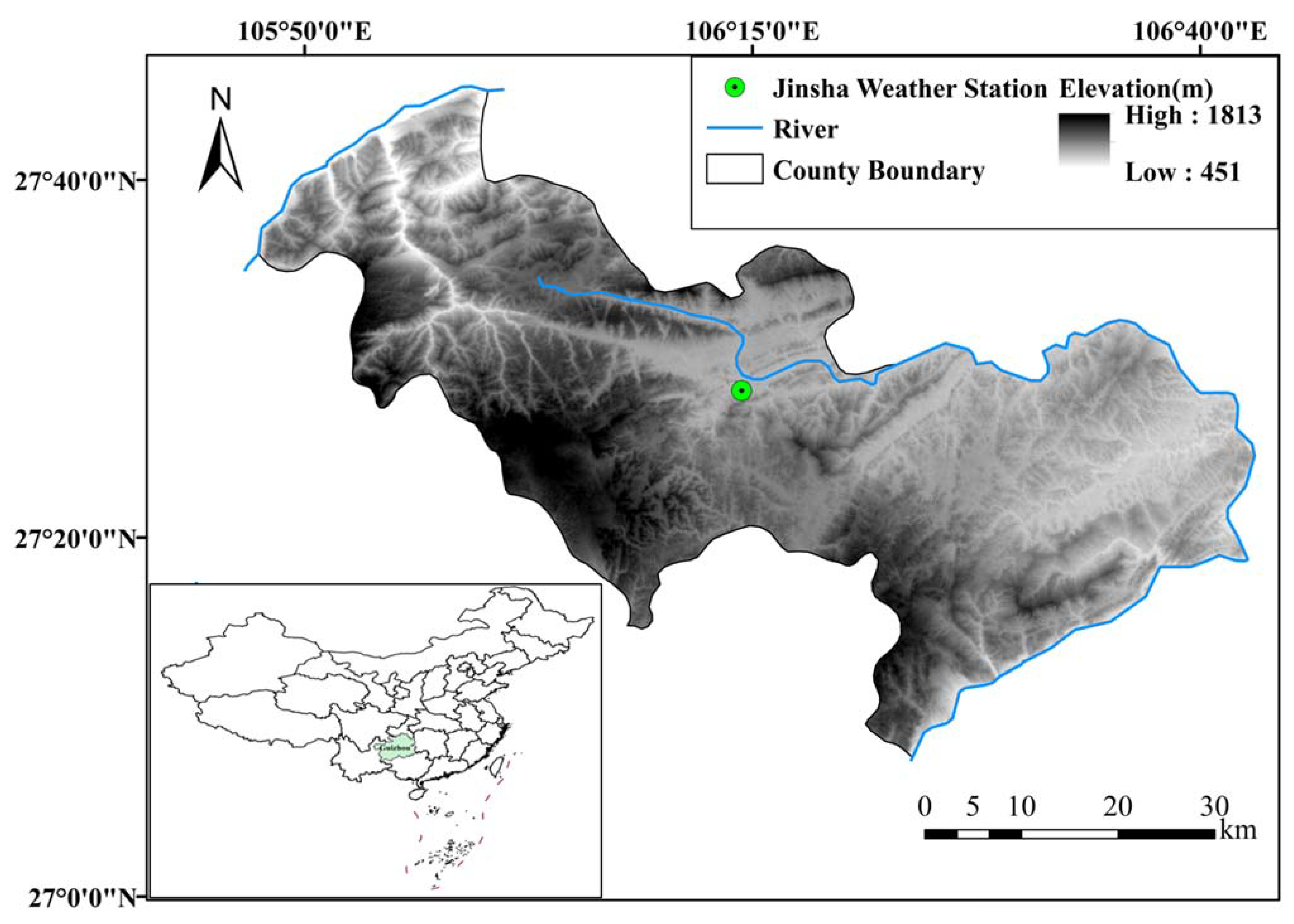
In this paper, annual precipitation data measured at Jinsha weather station, Chishui River located in the northwest of Guizhou Province were used. Figure 1 displays the location of the study area. The average annual precipitation of the Chishui River Basin is 800–1200 mm, and the average surface precipitation depth is 1020.6 mm. Abundant precipitation, frequent torrential rain events, and a fragile geological environment lead to the frequent occurrence of debris flow, landslide, and other mountain torrents. Therefore, it is of practical significance to forecast precipitation in this area for flood control, disaster reduction, and agricultural production.
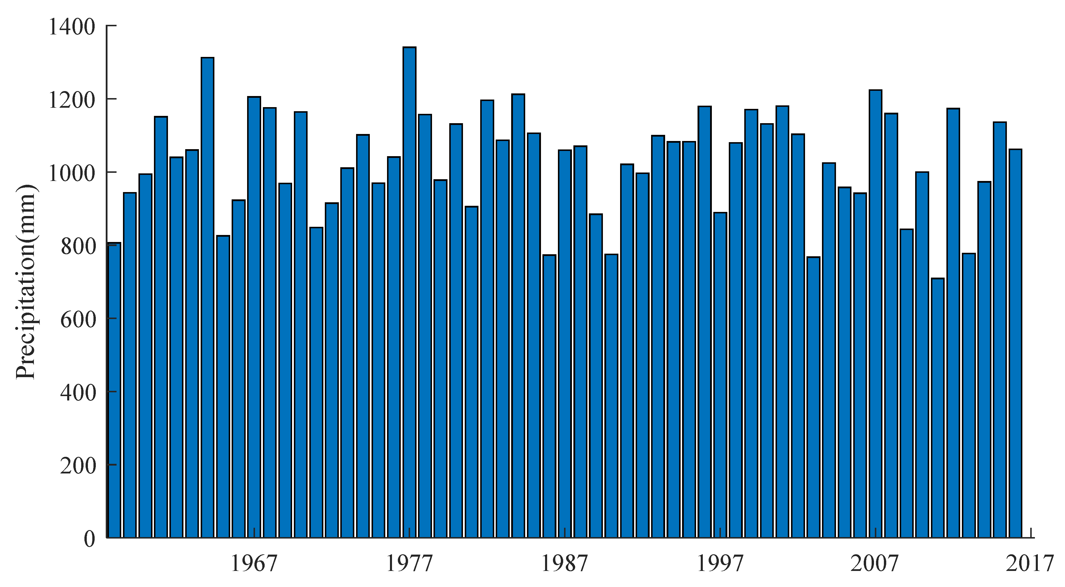
The annual rainfall data from 1958 to 2016 were employed. Figure 2 shows the original data for Jinsha station, data from 1958 to 2011 were adopted for training and those from 2012 to 2016 were used for testing. Statistical parameters of the original data are listed in Table 1. It can be observed that the original data shows obvious skewness, indicating a high difficulty of modeling.
2.2. Wavelet Packet Decomposition WPD
WPD is similar to WD, yet the former complements the defect of WD [44]. A three-layer binary tree structure of WPD is shown in Figure 3. WPD decomposes the signal into approximation coefficients and detail coefficients by a mother wavelet function. The decomposition level and mother wavelet function has a significant influence on the performance of WPD. WPD comprises continuous wavelet transform (CWT) and discrete wavelet transform (DWT). CWT is expressed as follows:
where is the input signal, a is the scale parameter, b is the translation parameter, ∗ is the complex conjugate, is the mother wavelet function. and in the DWT are expressed as:
where and are the scale parameter and translation parameter, respectively.
2.3. Extreme Learning Machine (ELM)
The ELM proposed by Huang et al. [45] is a single hidden layer feed-forward network (SLFN), which is a modified version of a traditional ANN with the characteristic of no adjustment made on internal parameters [46]. The ELM selects the hidden threshold randomly in training the network. The computation of output weight does not need complicated iteration, which greatly enhances the training speed.
For a vector (), , , ELM can be modeled by:
where denotes the weight connecting the nodes of the hidden layer and output layer, denotes the activation function, denotes the weight vector connecting the nodes of the input layer and output layer, denotes input vectors, denotes the threshold of the hidden node, denotes the output value, and denotes the number of hidden nodes.
The goal of the ELM is to minimize the error between the original and predicted values, , there exist , and . So,
Equation (4) can be expressed by the following equation:
where:
H stands for the output matrix of hidden nodes, is the output weight, Y is the target output. Thus the minimum norm least-squares solution of Equation (5) is:
where represents the Moore-Penrose generalized inverse (MPGI) of H and Y is the target.
2.4. Back-Propagation Neural Network (BPNN)
The BPNN proposed by McClelland and Rumelhart [47] is a common multilayered ANN. BPNN includes input nodes, hidden layers, and output layers. The characteristic of BPNN is the forward transmission of the signal and the reverse transmission of the error. BPNN minimizes the global error according to the gradient descent approach [48]. The connection weights are modified based on errors between the input and output data in the reverse transmission. Forward and backward propagation is repeated until the errors reach the expected precision. In this study, the Levenberg-Marquardt (LM) method, sigmoid function, and the purelin formula were adopted as the training function, transfer function, and output function, respectively. The mathematical formula of the BPNN model can be expressed as follows:
where represents the input data of node in layer m − 1, is weight of , is the bias of layer m, is the output value of node i in layer m; denotes the transfer function of layer m, which can be written as:
The purelin formula is expressed as follows:
2.5. ARIMA
ARIMA, proposed by Box [49], is normally utilized in time series analysis. The mathematical forecasting equation of ARIMA is linear, in which the predictors include autoregressive (AR) terms and moving average (MA) terms. The representation of ARIMA is ARIMA (p, d, q), and the representation of SARIMA (seasonal ARIMA) is ARIMA (p, d, q) × (P, D, Q)s, where (p, d, q) represents the non-seasonal order and (P, D, Q)s denotes the seasonal order. The ARIMA [50] model can be expressed as:
where is the time series, is the AR coefficient, is the MA coefficient, is the model parameter, p is the order of AR component, q is the order of MA component, and d is the order of differentiation.
2.6. Framework of the Proposed Hybrid Model
The architecture of the hybrid precipitation prediction framework (WPD-ELM) is presented in Figure 4. Detailed steps of the model are indicated as follows:
Step 1: Data pre-processing. (a) WPD was adopted to decompose the original precipitation series into several sub-series; (b) data (both in original series and sub-series) were partitioned into training and testing sets; (c) all data were tested by the Augmented Dickey-fuller Test (ADF); (d) normalize all data within [0, 1] by:
where is the original data, is the normalized data series, n the number of data.
Step 2: Model building. (a) partial autocorrelation function (PACF) and precipitation theory were employed to select the number of input variables; (b) values of the model parameters, such as the number of hidden layers in ANN and the optimized parameters for ARIMA, were set; (c) ELM, ARIMA, and BPNN were used as forecasting tools to model and predict each decomposed sub-sequence separately; (d) the results were integrated to produce the final prediction.
2.7. Evaluation Indicators
Results of the models were evaluated with respect to four evaluation indicators. These indexes included root mean square errors (RMSE) [51], mean absolute error (MAE) [52], Nash-Sutcliffe efficiency coefficient (NSEC) [53], and coefficient of correlation (R). Their equations are provided below.
where , , and are the estimated, observed, mean estimated, and mean observed values of precipitation, respectively.
3. Results
3.1. Decomposition Results
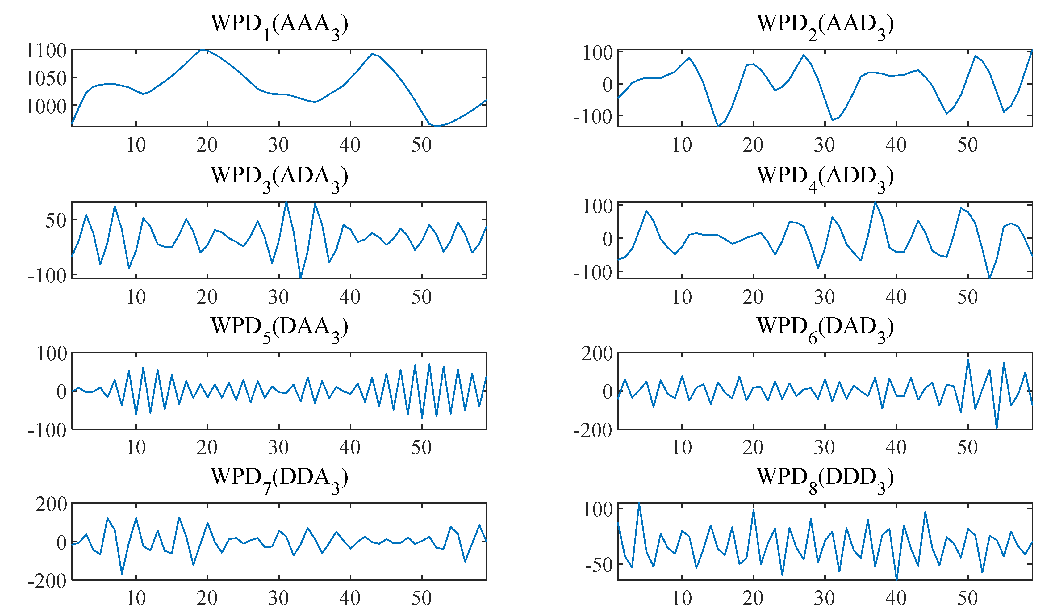
WPD was adopted to split the original annual precipitation data into several sub-series. The frequency of the sub-series was different, and each sub-series played a different role in the original dataset. The decomposed results for the Jinsha weather station using WPD at level 3 are shown in Figure 5.
3.2. Selection of Input Variable
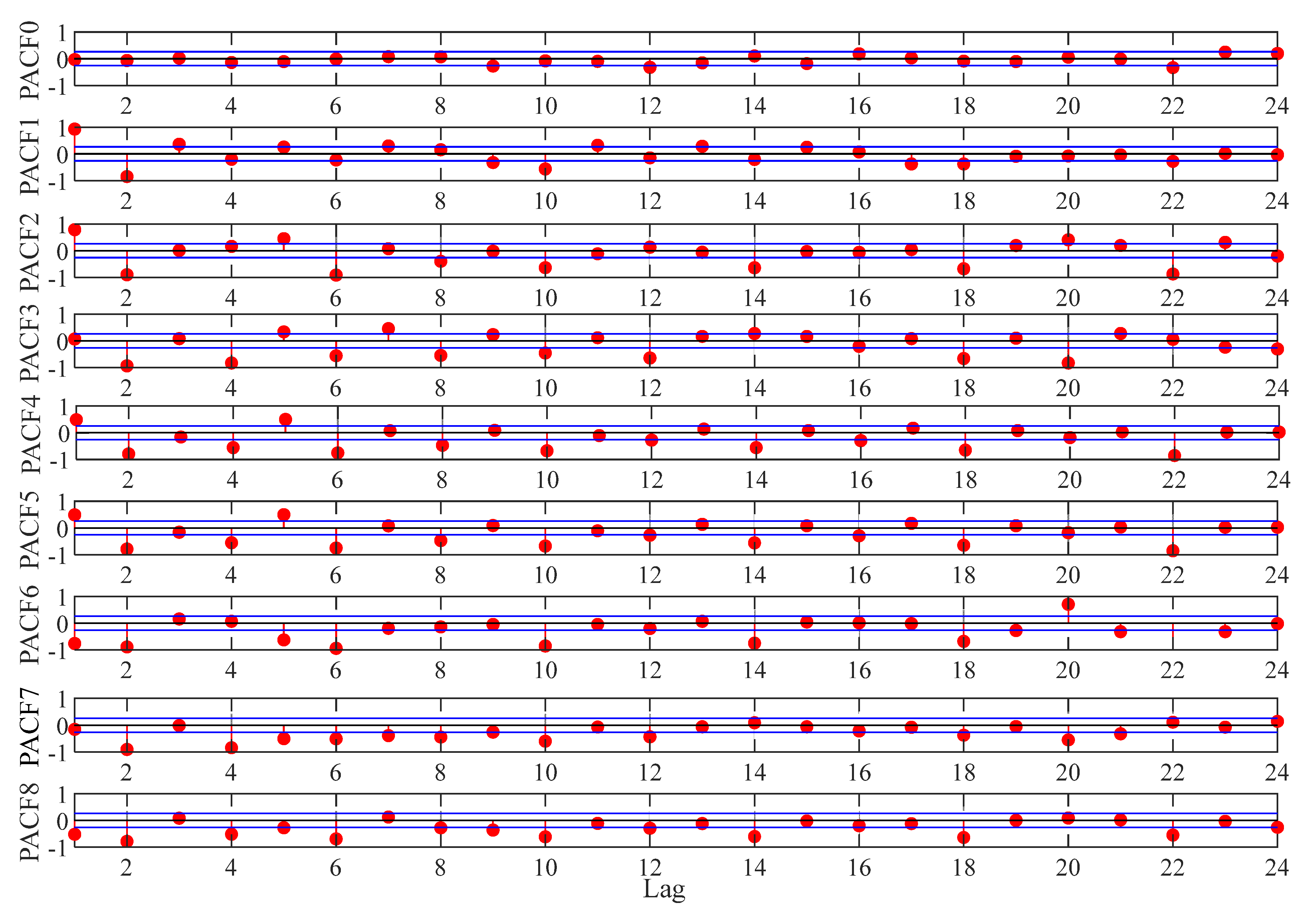
The selection of input variables has a significant effect on the prediction results. In this paper, two methods were utilized to select input combinations: (a) trial-and-error method; (b) PACF statistical approach. PACF values for all series from the Jinsha weather station are shown in Figure 6, where PACF0 denotes the original rainfall series and others are for the sub-series. Twelve ANN models with different input combinations were employed. Table 1 lists the input variables for different series with respect to the information in Figure 6 and the trial-and-error method, where represents the estimated value of rainfall and is the rainfall at time t − p.
3.3. Model Development
To verify the WPD-ELM model, six models, namely ELM, BPNN, ARIMA, WPD-ELM, WPD-BPNN, WPD-ARIMA, were employed for benchmark comparison. Detailed information relating to these models is described in this section.
- (1)
- ELM and BPNN models
For conventional ELM and BPNN models, the observed precipitation values are adopted as the target value. The number of nodes in the input and output layers is equal to the number of input variables and one, respectively. The best number of nodes in the hidden layer is determined by the trial-and-error method. In this paper, the best numbers of nodes in the hidden layer in the ELM and BPNN were set to twenty and eight, respectively. The LM algorithm is adopted to train the BPNN model and the training epoch was set to 500. The sigmoidal function was selected as the activation function of the ELM and the MPGI method was adopted to determine the hidden output weights after randomly setting its hidden threshold and weight vector between the hidden and input layers.
- (2)
- ARIMA
The Augmented Dickey-Fuller (ADF) unit root test was first employed to judge the stationarity of the input series. If the dataset was nonstationary, the difference and MA could be used to smooth it. The results are shown in Table 2. Value h = 1 means that the test rejects the null hypothesis of a unit root. The significance level of the p-value was determined as 0.05. Thus, when the t-statistic value was less than the critical value and the p-value < 0.05, the test results could be considered feasible and it would reject the null hypothesis. It can be seen from Table 2 that the sample dataset was stationary without a single root effect. Subsequently, the optimal ARIMA (p, d, q) structure was mainly determined according to the minimum Bayes information criteria (BIC) value. The resulting ARIMA models are shown in Table 3.
- (3)
- WPD-ANN and WPD-ARIMA
For WPD-ELM, WPD-BPNN, and WPD-ARIMA models, the original precipitation is split into eight sub-series using WPD, and several special hybrid models are reconstructed for each subsequence. For the WPD method, the selection of an appropriate wavelet basis function is very significant. The symlet wavelet is an improved approximate symmetric wavelet function based on Daubechies wavelet, which can avoid signal distortion during decomposition and reconstruction. Thus, a three-scale and four-order Symlet wavelet was considered as the wavelet basis function in this paper.
3.4. Comparative Analysis
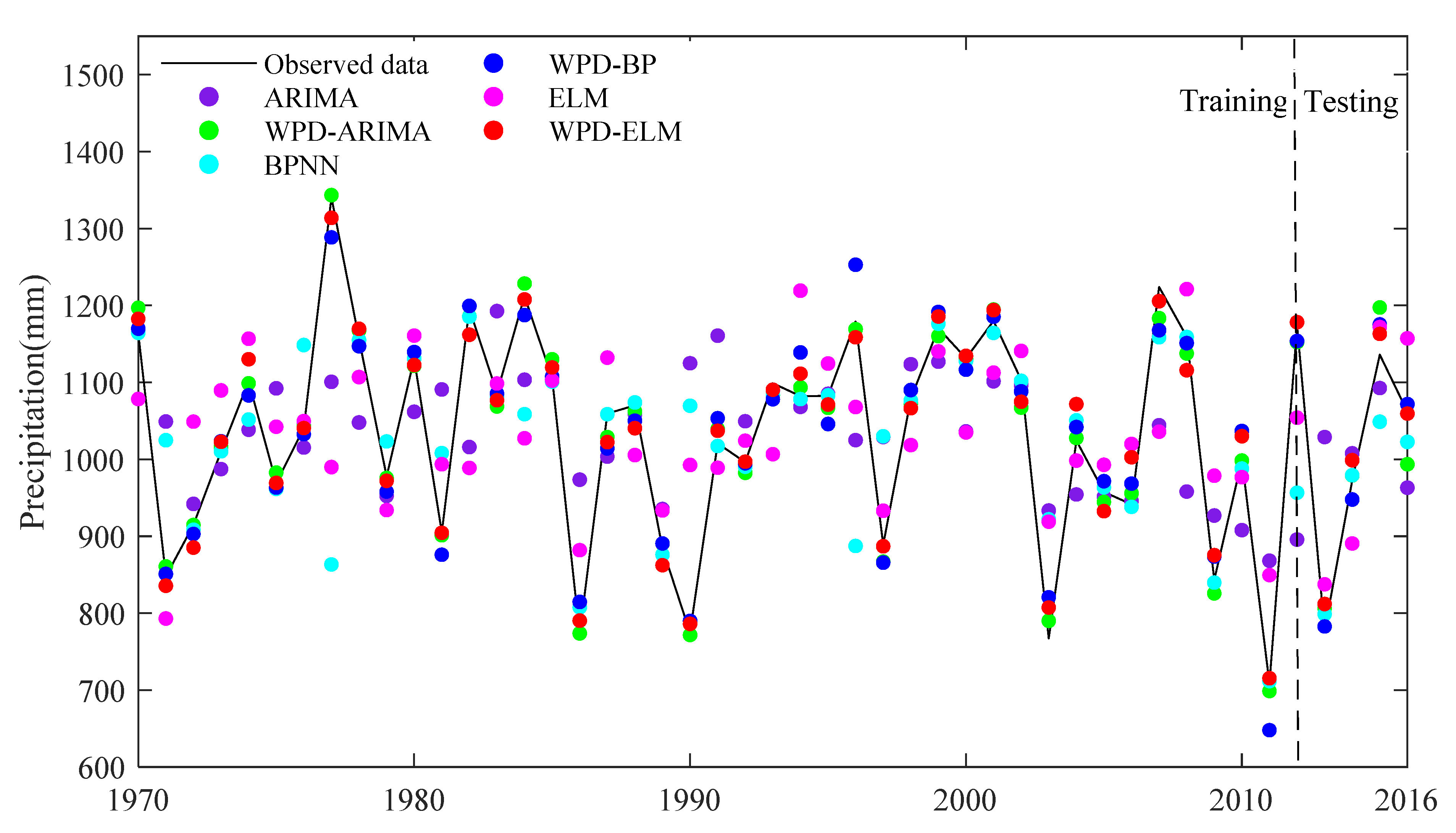
The forecast of the series was implemented using the above models with the input data of original annual precipitation and extracted subseries. The assessment results obtained by different models in training and test phases are shown in Table 4 and Table 5. Figure 7 exhibits the forecasting results using the six models.
One can see from Table 4 that when forecasting the annual precipitation in the Jinsha weather station, WPD-ELM could attain the best results in terms of four evaluation indexes. For example, in the testing period, the proposed hybrid model exhibited the highest R (0.997) and NSEC (0.973) and exhibited the lowest RMSE (23.069) and MAE (19.051). Compared with the prediction accuracy of six models in the training period, WPD-ARIMA provided the best results in terms of four evaluation indexes, the performance of WPD-ELM was slightly lower than WPD-ARIMA.
Table 5 lists the improvements obtained by several models. In the training period, WPD-ELM improved the ELM model with a 77.69% and 78.33% reduction in MAE and RMSE, respectively. Besides, improvements in prediction results regarding the NSEC and R were 146.35% and 56.91%, respectively. In the testing period, compared to the ELM model, WPD-ELM yielded reductions in terms of MAE and RMSE with 75.78% and 72.44%, respectively. Besides, the improvements in the forecasting results of WPD-ELM regarding the NSEC and R were 49.89% and 21.66%, respectively. Compared with the WPD-BPNN and WPD-ELM models, WPD-ARIMA could exhibit the best improvements in terms of all measures during both training and testing periods. Meanwhile, we could see that the improvements of WPD-BPNN were superior to WPD-ELM, whilst there was no dramatic difference between them.
The following conclusions could be drawn based on this analysis: (a) when comparing the performance of three single models with three hybrid models, the hybrid models attained better performance during both training and testing periods; (b) ELM outperformed the other single methods; (c) WPD-ARIMA demonstrated the optimal performance in terms of all measures in the training period, and WPD-ELM attained the best forecasting accuracy in terms of four evaluation indexes during the testing phase; (d) ARIMA provided the worst results during both training and testing periods; (e) there was no significant difference in the forecasting accuracy between BPNN and ELM and those between WPD-BPNN and WPD-ELM.
In addition, the prediction accuracy was different in terms of different phrases. The performance of the ARIMA method during the testing period was far inferior to that during the training period. The WPD-ARIMA model was of the highest level in the training period, but the performance in the testing period was the worst among several hybrid models, which meant the generalization ability of WPD-ARIMA was very poor. However, it was considered that the model had strong generalization capability for reliable performance when it performed modestly during the training period and well in the testing period, e.g., BPNN, WPD-BPNN, ELM, WPD-ELM.
The performances of all forecasting models developed in this paper during the training and testing phases are shown in Figure 7. One can clearly see that the performances of the hybrid models were better than those single methods as their trend lines were very close to the original data line. Meanwhile, the algorithm prior to the improvements had difficulty capturing the drastic changes in rainfall.
3.5. Discussion of Results
The following should be considered before analyzing the results. The forecasting performance of the testing phase plays a greater role than that of the training phase because the training phase is utilized to train the model, and its performance is measured by the data related to the modeling. However, the testing dataset does not participate in modeling, so its performance can truly reflect the model application efficiency. Based on the above considerations, we can draw the following conclusions from the above analysis. Firstly, the WPD-ELM model proposed in this paper can attain the best performance in terms of all statistical measures. Secondly, WPD is suitable for decomposing the annual precipitation series as it can overcome the complicated abrupt change of precipitation. Thirdly, there are obvious differences between the accuracies of the ARIMA, BPNN, and ELM models, which highlight the significant role of the training tool in modeling. Finally, the annual rainfall series decomposed by WPD as input in modeling can substantially enhance forecasting accuracy.
The WPD-ELM model outperforms all compared models. The reasons why the novel method can improve the accuracy are analyzed below. Firstly, WPD decomposes the original data into more linear subseries, reducing the modeling difficulty. Secondly, the ELM is employed to model the input-output relationship in each subsequence. The random initialization of the feature mapping parameters in the algorithm enhances the mutual independence of each input signal, creates a larger solution space, and improves the generalization ability. Finally, the WPD-ELM hybrid model overcomes the shortcomings of the single model by generating a synergistic effect in prediction.
Besides, this paper investigates the performance of WPD-ELM in annual precipitation forecasting. There are still several research directions to fill the research gap in future work. The first is to study an appropriate optimization algorithm to improve the performance of the WPD-ELM model. The study is carried out based on a limited dataset, so the second is to test the generalization of the proposed model. Due to uncertainties caused by the stochastic processes in the neural network model, the last major issue is to solve the problem of randomness. In future research, it is necessary to conduct in-depth research on the above three aspects to study a more accurate prediction model and make contributions to the field of hydrological forecasting.
4. Conclusions
Improving the accuracy of long-term annual precipitation forecasting is an important yet challenging work in water resources management. We propose a novel hybrid precipitation prediction framework (WPD-ELM). Firstly, WPD is adopted to decompose the original annual precipitation series into several sub-series. Secondly, ANN models are utilized to predict each sub-series. Finally, results are integrated to produce the final prediction. The annual precipitation series gathered at the Jinsha weather station of Guizhou Province in China are taken to develop the empirical study. Results indicate that WPD-ELM outperforms other benchmark methods in this paper in terms of four evaluation indicators. Meanwhile, the performances of the hybrid models are better than those of the standard BPNN, ARIMA, and ELM, which means that WPD can significantly improve the forecasting accuracy. In conclusion, WPD can be used to preprocess precipitation data and WPD-ELM can provide more accurate and reliable results, thus, it may be a promising alternative for long-term precipitation prediction.
Author Contributions
Methodology, Software, Writing—original draft: H.W.; Conceptualization, Writing—original draft: W.W.; Program implementation, Writing—original draft: Y.D.; Formal analysis: D.X. All authors have read and agreed to the published version of the manuscript.
Funding
Project of key science and technology of the Henan province (202102310259; 202102310588), and Henan province university scientific and technological innovation team (No:18IRTSTHN009).
Institutional Review Board Statement
Not applicable.
Informed Consent Statement
Not applicable.
Data Availability Statement
All authors made sure that all data and materials support our published claims and comply with field standards.
Acknowledgments
The authors are grateful to two anonymous reviewers and editors for providing valuable comments and suggestion, which we considered to improve the quality of this paper. The authors are grateful to Chau Kwok-wing to help to revise the conceptualization, language, and syntax errors of the manuscript.
Conflicts of Interest
The authors declare that they have no conflict of interest.
References
- Wei, H.; Li, J.-L.; Liang, T.-G. Study on the estimation of precipitation resources for rainwater harvesting agriculture in semi-arid land of China. Agric. Water Manag. 2005, 71, 33–45. [Google Scholar] [CrossRef]
- Wang, W.-C.; Xu, D.-M.; Chau, K.-W.; Chen, S. Improved annual rainfall-runoff forecasting using PSO-SVM model based on EEMD. J. Hydroinformatics 2013, 15, 1377–1390. [Google Scholar] [CrossRef]
- Kisi, O.; Cimen, M. A wavelet-support vector machine conjunction model for monthly streamflow forecasting. J. Hydrol. 2011, 399, 132–140. [Google Scholar] [CrossRef]
- Wang, X.; Kinsland, G.; Poudel, D.; Fenech, A. Urban flood prediction under heavy precipitation. J. Hydrol. 2019, 577, 123984. [Google Scholar] [CrossRef]
- Hartmann, H.; Snow, J.A.; Su, B.; Jiang, T. Seasonal predictions of precipitation in the Aksu-Tarim River basin for improved water resources management. Glob. Planet. Chang. 2016, 147, 86–96. [Google Scholar] [CrossRef]
- Nguyen, D.H.; Bae, D.-H. Correcting mean areal precipitation forecasts to improve urban flooding predictions by using long short-term memory network. J. Hydrol. 2020, 584, 124710. [Google Scholar] [CrossRef]
- Benedetto, A. A decision support system for the safety of airport runways: The case of heavy rainstorms. Transp. Res. Part. A Policy Pract. 2002, 36, 665–682. [Google Scholar] [CrossRef]
- Kuligowski, R.J.; Barros, A.P. Experiments in Short-Term Precipitation Forecasting Using Artificial Neural Networks. Mon. Weather. Rev. 1998, 126, 470–482. [Google Scholar] [CrossRef]
- Ortiz-García, E.G.; Salcedo-Sanz, S.; Casanova-Mateo, C. Accurate precipitation prediction with support vector classifiers: A study including novel predictive variables and observational data. Atmos. Res. 2014, 139, 128–136. [Google Scholar] [CrossRef]
- Box, G.E.P.; Jenkins, G.M.; Reinsel, G.C. Time Series Analysis: Forecasting and Control, 3rd ed.; Prentice Hall: Englewood Cliffs, NJ, USA, 1994. [Google Scholar]
- Mohammadi, K.; Eslami, H.R.; Kahawita, R. Parameter estimation of an ARMA model for river flow forecasting using goal programming. J. Hydrol. 2006, 331, 293–299. [Google Scholar] [CrossRef]
- Pektaş, A.O.; Kerem Cigizoglu, H. ANN hybrid model versus ARIMA and ARIMAX models of runoff coefficient. J. Hydrol. 2013, 500, 21–36. [Google Scholar] [CrossRef]
- Wang, W.-C.; Chau, K.-W.; Cheng, C.-T.; Qiu, L. A comparison of performance of several artificial intelligence methods for forecasting monthly discharge time series. J. Hydrol. 2009, 374, 294–306. [Google Scholar] [CrossRef] [Green Version]
- Dhote, V.; Mishra, S.; Shukla, J.P.; Pandey, S.K. Runoff prediction using Big Data analytics based on ARIMA Model. Indian J. Geo-Mar. Sci. 2018, 47, 2163–2170. [Google Scholar]
- Valipour, M.; Banihabib, M.E.; Behbahani, S.M.R. Comparison of the ARMA, ARIMA, and the autoregressive artificial neural network models in forecasting the monthly inflow of Dez dam reservoir. J. Hydrol. 2013, 476, 433–441. [Google Scholar] [CrossRef]
- Burlando, P.; Rosso, R.; Cadavid, L.G.; Salas, J.D. Forecasting of short-term rainfall using ARMA models. J. Hydrol. 1993, 144, 193–211. [Google Scholar] [CrossRef]
- Wu, C.L.; Chau, K.W. Prediction of rainfall time series using modular soft computingmethods. Eng. Appl. Artif. Intell. 2013, 26, 997–1007. [Google Scholar] [CrossRef] [Green Version]
- Zhu, L.; Wang, Y.; Fan, Q. MODWT-ARMA model for time series prediction. Appl. Math. Model. 2014, 38, 1859–1865. [Google Scholar] [CrossRef]
- Papalaskaris, T.; Panagiotidis, T.; Pantrakis, A. Stochastic Monthly Rainfall Time Series Analysis, Modeling and Forecasting in Kavala City, Greece, North-Eastern Mediterranean Basin. Procedia Eng. 2016, 162, 254–263. [Google Scholar] [CrossRef] [Green Version]
- Mahmud, I.; Bari, S.H.; Rahman, M.T.U. Monthly rainfall forecast of Bangladesh using autoregressive integrated moving average method. Environ. Eng. Res. 2017, 22, 162–168. [Google Scholar] [CrossRef] [Green Version]
- Al Balasmeh, O.; Babbar, R.; Karmaker, T. Trend analysis and ARIMA modeling for forecasting precipitation pattern in Wadi Shueib catchment area in Jordan. Arab. J. Geosci. 2019, 12. [Google Scholar] [CrossRef]
- Hung, N.Q.; Babel, M.S.; Weesakul, S.; Tripathi, N.K. An artificial neural network model for rainfall forecasting in Bangkok, Thailand. Hydrol. Earth Syst. Sci. 2009, 13, 1413–1425. [Google Scholar] [CrossRef] [Green Version]
- Nastos, P.T.; Paliatsos, A.G.; Koukouletsos, K.V.; Larissi, I.K.; Moustris, K.P. Artificial neural networks modeling for forecasting the maximum daily total precipitation at Athens, Greece. Atmos. Res. 2014, 144, 141–150. [Google Scholar] [CrossRef]
- Abbot, J.; Marohasy, J. Input selection and optimisation for monthly rainfall forecasting in Queensland, Australia, using artificial neural networks. Atmos. Res. 2014, 138, 166–178. [Google Scholar] [CrossRef]
- Abbot, J.; Marohasy, J. Skilful rainfall forecasts from artificial neural networks with long duration series and single-month optimization. Atmos. Res. 2017, 197, 289–299. [Google Scholar] [CrossRef]
- Pham, B.T.; Le, L.M.; Le, T.-T.; Bui, K.-T.T.; Le, V.M.; Ly, H.-B.; Prakash, I. Development of advanced artificial intelligence models for daily rainfall prediction. Atmos. Res. 2020, 237, 104845. [Google Scholar] [CrossRef]
- Feng, Q.; Wen, X.H.; Li, J.G. Wavelet Analysis-Support Vector Machine Coupled Models for Monthly Rainfall Forecasting in Arid Regions. Water Resour. Manag. 2015, 29, 1049–1065. [Google Scholar] [CrossRef]
- Balasubramanian, G.; Kanagasabai, A.; Mohan, J.; Seshadri, N.P.G. Music induced emotion using wavelet packet decomposition—An EEG study. Biomed. Signal. Process. Control. 2018, 42, 115–128. [Google Scholar] [CrossRef]
- Kisi, O. Wavelet regression model for short-term streamflow forecasting. J. Hydrol. 2010, 389, 344–353. [Google Scholar] [CrossRef]
- Kisi, O.; Cimen, M. Precipitation forecasting by using wavelet-support vector machine conjunction model. Eng. Appl. Artif. Intell. 2012, 25, 783–792. [Google Scholar] [CrossRef]
- Zhou, H.-C.; Peng, Y.; Liang, G.-H. The Research of Monthly Discharge Predictor-corrector Model Based on Wavelet Decomposition. Water Resour. Manag. 2008, 22, 217–227. [Google Scholar] [CrossRef]
- Zhang, Q.; Wang, B.-D.; He, B.; Peng, Y.; Ren, M.-L. Singular Spectrum Analysis and ARIMA Hybrid Model for Annual Runoff Forecasting. Water Resour. Manag. 2011, 25, 2683–2703. [Google Scholar] [CrossRef]
- Karthikeyan, L.; Nagesh Kumar, D. Predictability of nonstationary time series using wavelet and EMD based ARMA models. J. Hydrol. 2013, 502, 103–119. [Google Scholar] [CrossRef]
- Venkata Ramana, R.; Krishna, B.; Kumar, S.R.; Pandey, N.G. Monthly Rainfall Prediction Using Wavelet Neural Network Analysis. Water Resour. Manag. 2013, 27, 3697–3711. [Google Scholar] [CrossRef] [Green Version]
- Partal, T.; Cigizoglu, H.K.; Kahya, E. Daily precipitation predictions using three different wavelet neural network algorithms by meteorological data. Stoch. Environ. Res. Risk Assess. 2015, 29, 1317–1329. [Google Scholar] [CrossRef]
- Abdourahamane, Z.S.; Acar, R.; Serkan, S. Wavelet-copula-based mutual information for rainfall forecasting applications. Hydrol. Process. 2019, 33, 1127–1142. [Google Scholar] [CrossRef]
- Chong, K.L.; Lai, S.H.; Yao, Y.; Ahmed, A.N.; Jaafar, W.Z.W.; El-Shafie, A. Performance Enhancement Model for Rainfall Forecasting Utilizing Integrated Wavelet-Convolutional Neural Network. Water Resour. Manag. 2020, 34, 2371–2387. [Google Scholar] [CrossRef]
- Ben messaoud, M.a.; Bouzid, A.; Ellouze, N. Speech enhancement based on wavelet packet of an improved principal component analysis. Comput. Speech Lang. 2016, 35, 58–72. [Google Scholar] [CrossRef]
- Yu, C.; Li, Y.; Xiang, H.; Zhang, M. Data mining-assisted short-term wind speed forecasting by wavelet packet decomposition and Elman neural network. J. Wind Eng. Ind. Aerodyn. 2018, 175, 136–143. [Google Scholar] [CrossRef]
- Liu, H.; Mi, X.; Li, Y. Comparison of two new intelligent wind speed forecasting approaches based on Wavelet Packet Decomposition, Complete Ensemble Empirical Mode Decomposition with Adaptive Noise and Artificial Neural Networks. Energy Convers. Manag. 2018, 155, 188–200. [Google Scholar] [CrossRef]
- Seo, Y.; Kim, S.; Kisi, O.; Singh, V.P.; Parasuraman, K. River Stage Forecasting Using Wavelet Packet Decomposition and Machine Learning Models. Water Resour. Manag. 2016, 30, 4011–4035. [Google Scholar] [CrossRef]
- Guo, Z.; Zhao, W.; Lu, H.; Wang, J. Multi-step forecasting for wind speed using a modified EMD-based artificial neural network model. Renew. Energy 2012, 37, 241–249. [Google Scholar] [CrossRef]
- Tan, Q.-F.; Lei, X.-H.; Wang, X.; Wang, H.; Wen, X.; Ji, Y.; Kang, A.-Q. An adaptive middle and long-term runoff forecast model using EEMD-ANN hybrid approach. J. Hydrol. 2018, 567, 767–780. [Google Scholar] [CrossRef]
- Alickovic, E.; Kevric, J.; Subasi, A. Performance evaluation of empirical mode decomposition, discrete wavelet transform, and wavelet packed decomposition for automated epileptic seizure detection and prediction. Biomed. Signal. Process. Control. 2018, 39, 94–102. [Google Scholar] [CrossRef]
- Guang-Bin, H.; Qin-Yu, Z.; Chee-Kheong, S. Extreme learning machine: A new learning scheme of feedforward neural networks. In Proceedings of the 2004 IEEE International Joint Conference on Neural Networks (IEEE Cat. No.04CH37541), Budapest, Hungary, 25–29 July 2004; Volume 982, pp. 985–990. [Google Scholar]
- Yaseen, Z.M.; Sulaiman, S.O.; Deo, R.C.; Chau, K.W. An enhanced extreme learning machine model for river flow forecasting: State-of-the-art, practical applications in water resource engineering area and future research direction. J. Hydrol. 2019, 569, 387–408. [Google Scholar] [CrossRef]
- McCelland, J.; Rumelhart, D. Parallel Distributed Processing; MIT Press: Cambridge, MA, USA, 1986. [Google Scholar]
- Wang, J.J.; Shi, P.; Jiang, P.; Hu, J.W.; Qu, S.M.; Chen, X.Y.; Chen, Y.B.; Dai, Y.Q.; Xiao, Z.W. Application of BP Neural Network Algorithm in Traditional Hydrological Model for Flood Forecasting. Water 2017, 9, 48. [Google Scholar] [CrossRef] [Green Version]
- Box, G. Box and Jenkins: Time Series Analysis, Forecasting and Control. In A Very British Affair: Six Britons and the Development of Time Series Analysis during the 20th Century; Mills, T.C., Ed.; Palgrave Macmillan UK: London, UK, 2013; pp. 161–215. [Google Scholar]
- Wang, W.-c.; Chau, K.-w.; Xu, D.-m.; Chen, X.-Y. Improving Forecasting Accuracy of Annual Runoff Time Series Using ARIMA Based on EEMD Decomposition. Water Resour. Manag. 2015, 29, 2655–2675. [Google Scholar] [CrossRef]
- Gentilucci, M.; Materazzi, M.; Pambianchi, G.; Burt, P.; Guerriero, G. Assessment of Variations in the Temperature-Rainfall Trend in the Province of Macerata (Central Italy), Comparing the Last Three Climatological Standard Normals (1961–1990; 1971–2000; 1981–2010) for Biosustainability Studies. Environ. Process. 2019, 6, 391–412. [Google Scholar] [CrossRef]
- Willmott, C.; Matsuura, K. Advantages of the Mean Absolute Error (MAE) over the Root Mean Square Error (RMSE) in Assessing Average Model Performance. Clim. Res. 2005, 30, 79. [Google Scholar] [CrossRef]
- Kim, H.I.; Keum, H.J.; Han, K.Y. Real-Time Urban Inundation Prediction Combining Hydraulic and Probabilistic Methods. Water 2019, 11, 293. [Google Scholar] [CrossRef] [Green Version]
Figure 1.
Location of Jinsha weather station.

Figure 2.
Original annual precipitation data of Jinsha weather station.

Figure 3.
Schematic diagram of the Wavelet Packet Decomposition (WPD) method.

Figure 4.
Framework of the proposed hybrid model.

Figure 5.
Decomposed results for annual rainfall in Jinsha station.

Figure 6.
Partial autocorrelation function (PACF) values for different series.

Figure 7.
Observed and forecasted results during training and testing periods by six methods.


Table 1.
Input variables for different series.
| No. | Series | Input Variables |
|---|---|---|
| 1 | original | q(t−1)~q(t−9) |
| 2 | WPD1 | q(t−1)~q(t−12) |
| 3 | WPD2 | q(t−1)~q(t−11) |
| 4 | WPD3 | q(t−1)~q(t−11) |
| 5 | WPD4 | q(t−1)~q(t−12) |
| 6 | WPD5 | q(t−1)~q(t−12) |
| 7 | WPD6 | q(t−1)~q(t−10) |
| 8 | WPD7 | q(t−1)~q(t−10) |
| 9 | WPD8 | q(t−1)~q(t−9) |
Table 2.
Augmented Dickey-Fuller (ADF) test results.
| No. | Series | h | p-Value | t-Statistic | Critical Value |
|---|---|---|---|---|---|
| 1 | Original | 1 | 0 | −7.928 | −3.489 |
| 2 | WPD1 | 0 | 0.288 | −2.586 | −3.506 |
| 3 | Diff (WPD1) | 1 | 0.020 | −2.348 | −1.948 |
| 4 | WPD2 | 1 | 0 | −7.001 | −3.504 |
| 5 | WPD3 | 1 | 0.007 | −4.299 | −3.504 |
| 6 | WPD4 | 1 | 0 | −6.753 | −3.504 |
| 7 | WPD5 | 1 | 0.004 | −4.470 | −3.506 |
| 8 | WPD6 | 1 | 0 | −7.419 | −3.504 |
| 9 | WPD7 | 1 | 0 | −11.164 | −3.504 |
| 10 | WPD8 | 1 | 0 | −9.553 | −3.504 |
Table 3.
Auto-regressive integrated moving average (ARIMA) models based on BIC(Bayes information criteria).
Table 3.
Auto-regressive integrated moving average (ARIMA) models based on BIC(Bayes information criteria).
| No. | Series | ARIMA | BIC |
|---|---|---|---|
| 1 | Original | ARIMA (12,1,2) | 11.292 |
| 2 | WPD1 | ARIMA (9,1,3) | 4.026 |
| 3 | WPD2 | ARIMA (6,0,6) | 5.63 |
| 4 | WPD3 | ARIMA (7,0,5) | 5.494 |
| 5 | WPD4 | ARIMA (5,0,8) | 6.531 |
| 6 | WPD5 | ARIMA (2,0,7) | 3.076 |
| 7 | WPD6 | ARIMA (11,0,9) | 6.535 |
| 8 | WPD7 | ARIMA (12,0,5) | 6.435 |
| 9 | WPD8 | ARIMA (6,0,6) | 6.806 |
Table 4.
Prediction performance of different models in training and testing phases.
| Model | Training | Testing | ||||||
|---|---|---|---|---|---|---|---|---|
| R | NSEC | RMSE | MAE | R | NSEC | RMSE | MAE | |
| ARIMA | 0.415 | 0.139 | 129.978 | 101.046 | −0.304 | −0.535 | 175.136 | 141.295 |
| WPD-ARIMA | 0.991 | 0.981 | 19.399 | 14.951 | 0.951 | 0.903 | 44.127 | 37.199 |
| BPNN | 0.618 | 0.357 | 112.634 | 53.775 | 0.820 | 0.434 | 106.368 | 74.221 |
| WPD-BPNN | 0.978 | 0.957 | 29.445 | 22.924 | 0.988 | 0.973 | 23.176 | 19.947 |
| ELM | 0.628 | 0.394 | 109.308 | 85.583 | 0.819 | 0.649 | 83.698 | 78.656 |
| WPD-ELM | 0.986 | 0.9712 | 23.687 | 19.091 | 0.997 | 0.973 | 23.069 | 19.051 |
Table 5.
Comparison of model prediction performances.
| Model | Index | Training(%) | Testing(%) |
|---|---|---|---|
| WPD-ARIMA & ARIMA | R(↑) | 138.81 | 413.25 |
| NSEC(↑) | 607.65 | 268.63 | |
| RMSE(↓) | 85.08 | 74.80 | |
| MAE(↓) | 85.20 | 73.67 | |
| WPD-BPNN & BPNN | R(↑) | 58.14 | 20.43 |
| NSEC(↑) | 167.82 | 124.37 | |
| RMSE(↓) | 73.86 | 78.21 | |
| MAE(↓) | 57.37 | 73.12 | |
| WPD-ELM & ELM | R(↑) | 56.91 | 21.66 |
| NSEC(↑) | 146.35 | 49.89 | |
| RMSE(↓) | 78.33 | 72.44 | |
| MAE(↓) | 77.69 | 75.78 |
Note: where (↑) represents the percentage improvement of the previous model compared to the new model, and (↓) represents the percentage reduction and improvement of the previous model compared to the new model.
Publisher’s Note: MDPI stays neutral with regard to jurisdictional claims in published maps and institutional affiliations. |
© 2021 by the authors. Licensee MDPI, Basel, Switzerland. This article is an open access article distributed under the terms and conditions of the Creative Commons Attribution (CC BY) license (https://creativecommons.org/licenses/by/4.0/).
Share and Cite
MDPI and ACS Style
Wang, H.; Wang, W.; Du, Y.; Xu, D. Examining the Applicability of Wavelet Packet Decomposition on Different Forecasting Models in Annual Rainfall Prediction. Water 2021, 13, 1997. https://doi.org/10.3390/w13151997
AMA Style
Wang H, Wang W, Du Y, Xu D. Examining the Applicability of Wavelet Packet Decomposition on Different Forecasting Models in Annual Rainfall Prediction. Water. 2021; 13(15):1997. https://doi.org/10.3390/w13151997
Chicago/Turabian StyleWang, Hua, Wenchuan Wang, Yujin Du, and Dongmei Xu. 2021. "Examining the Applicability of Wavelet Packet Decomposition on Different Forecasting Models in Annual Rainfall Prediction" Water 13, no. 15: 1997. https://doi.org/10.3390/w13151997
Note that from the first issue of 2016, this journal uses article numbers instead of page numbers. See further details here.