
Optimal Water Quality Sensor Placement by Accounting for Possible Contamination Events in Water Distribution Networks


Department of Civil Engineering, Kyung Hee University, 1732 Deogyeong-daero, Giheung-gu, Yongin-si 17104, Korea
*
Author to whom correspondence should be addressed.
Water 2021, 13(15), 1999; https://doi.org/10.3390/w13151999
Submission received: 9 June 2021
/
Revised: 16 July 2021
/
Accepted: 18 July 2021
/
Published: 21 July 2021
(This article belongs to the Special Issue Active Contamination Event Detection in Water-Distribution Systems)
Abstract
:Contamination in water distribution networks (WDNs) can occur at any time and location. One protection measure in WDNs is the placement of water quality sensors (WQSs) to detect contamination and provide information for locating the potential contamination source. The placement of WQSs in WDNs must be optimally planned. Therefore, a robust sensor-placement strategy (SPS) is vital. The SPS should have clear objectives regarding what needs to be achieved by the sensor configuration. Here, the objectives of the SPS were set to cover the contamination event stages of detection, consumption, and source localization. As contamination events occur in any form of intrusion, at any location and time, the objectives had to be tested against many possible scenarios, and they needed to reach a fair value considering all scenarios. In this study, the particle swarm optimization (PSO) algorithm was selected as the optimizer. The SPS was further reinforced using a databasing method to improve its computational efficiency. The performance of the proposed method was examined by comparing it with a benchmark SPS example and applying it to DMA-sized, real WDNs. The proposed optimization approach improved the overall fitness of the configuration by 23.1% and showed a stable placement behavior with the increase in sensors.
1. Introduction
Implementing an efficient monitoring system is critical for water distribution networks (WDNs). Water quality sensor (WQS) placement is essential for maintaining WDN functionality and plays an integral part in preventing contamination events and ensuring the safety of distributed water to protect the health of users. Contamination occurs when hazardous contaminants are introduced into distributed water. There are several pathways for contaminants to enter distributed water, namely an accident in the system [1] or a deliberate attack on the network [2], with contaminants being able to enter the network at any stage of the distribution. If the contaminant is not detected quickly, it can cause significant health and economic losses. Hence, a proper sensor placement strategy (SPS) is required.
Deploying multiple WQSs will increase the robustness of the network in detecting contamination. However, owing to the high cost of sensor installation and maintenance, it is not practical to secure all individual network parts. It is more realistic to determine the placement location to detect contamination efficiently from a cost-effective standpoint. SPSs have been studied extensively and are typically developed using optimization formulations where the optimization involves many types of optimization objective that are solved through single-objective or multi-objective algorithms [3].
At the outset, this study was dominated by single-objective optimization with the approach aiming to optimize the SPS based on a single target criterion. Lee and Deininger introduced the maximum coverage objective and solved it using an integer programming (IP) model [4]. Later, a heuristic approach was applied using mixed-integer programming (MIP) by Kumar et al. [5] and a genetic algorithm (GA) by Al-Zahrani and Moeid [6]. Kessler et al. [7] applied the volume consumed before the detection as an objective, whilst Berry et al. [8] minimized the fraction of the exposed population using MIP. Later, multi-objective optimization was used. In this approach, many criteria that needed to be fulfilled for an SPS were defined. The optimization provided the singular best option or the Pareto front of the options. Watson et al. [9] considered a multi-objective approach using MIP. The approach focuses on the population exposed, time to detection, volume consumed, number of failed detections, and extent of contamination as the performance objectives. A similar set of objectives was employed by Wu and Walski [10] and solved using a GA.
Besides considering single or multiple objectives in SPS, other circumstances in the approach can include the network hydraulic or sensor characteristics. In Ostfeld and Salomon’s study [11], unsteady hydraulic and water quality conditions were considered using a GA framework paired with EPANET [12]. Sensor favored objectives of sensor detection likelihood, detection redundancy, and expected detection time were applied by Preis and Ostfeld using NSGA-II [13].
Optimal SPS is a complex problem and is affected by many parameters. A change in the contaminant source location and injection time could result in entirely different contamination spread behavior. Changes in sensor configuration, such as quantity and location, also vary the resulting accuracy in a non-linear manner. Quantifying the possible contamination scenarios and the candidate sensor configuration, the optimal SPS is an NP-hard combinatorial optimization [14]. Because of this, it is not practical to perform an exhaustive search, and a heuristic or metaheuristic method is preferred. In past studies, the typically used solvers are IP, MIP, GA, NSGA-II, and heuristic methods [3].
Despite the many advances in the field to date, there is still room for improvement and additional perspectives. Single-objective optimization guarantees the optimal solution for the said objective. However, it is not adequate to represent the optimality of sensor placement using a single objective function. The consequences of contamination will affect many aspects of WDNs. Therefore, different aspects should be considered to produce a balanced result. This balancing aspect must be addressed in multiple objective optimizations. As water demand changes throughout the day, the flow pathway characteristics also change, leading to many scenarios with different outcomes being considered. The use of GA or its variant NSGA-II as the optimization algorithm has been favored by many researchers [6,10,11,13]. However, it has some weaknesses in requiring more computational power along with the increase in problem complexity and sensitivity to chosen parameters.
In this study, three objectives with respect to contamination stages were chosen. The objectives considered the stages of contamination detection, contamination consumption, and source identification. They were applied to many scenarios with different contaminant source locations and times of intrusion combination. Hydraulic variability was also accounted for in the scenarios as water usage characteristics change over time. A method to save time and processing power was implemented through pre-simulation and databasing to remove hydraulic and water quality simulation needs throughout the optimization process. Particle swarm optimization (PSO) was chosen to bypass the GA’s computation efficiency shortcoming. PSO has been applied in the field of WDN design [15,16], with its performance compared to GA by Eberhart and Shi [17]. By applying all the described methods, this study aimed to provide a configurable method that utilize fewer resources and showcase the PSO algorithm adapted to solve the SPS. The method proposed in the study was named the sensor placement swarm optimizer (SPSO) method. Some limitations of this method need to be noted. The method was only tested against district metered areas (DMA) sized networks. The scalability to more extensive networks was not tested. As the scenarios were explicitly determined, no uncertainties were considered. Because SPSO is a simplified method, it loses some accuracy when compared to the stochastic method. Considering that contamination behaves differently depending on the contaminant type, this study only accounts for the presence of a contaminant in the network without consideration of contaminant species and reactions in the pipes.
The remainder of this paper proceeds as follows. Section 2 and Section 3 describe the methodology and objective functions used in the study in detail. An SPS in a network that has been used in past studies is used as a benchmark for the new method. The applicability of the proposed method is demonstrated in small DMA networks, as shown in Section 4. Finally, the conclusions of this study are presented in Section 5.
2. Materials and Methods
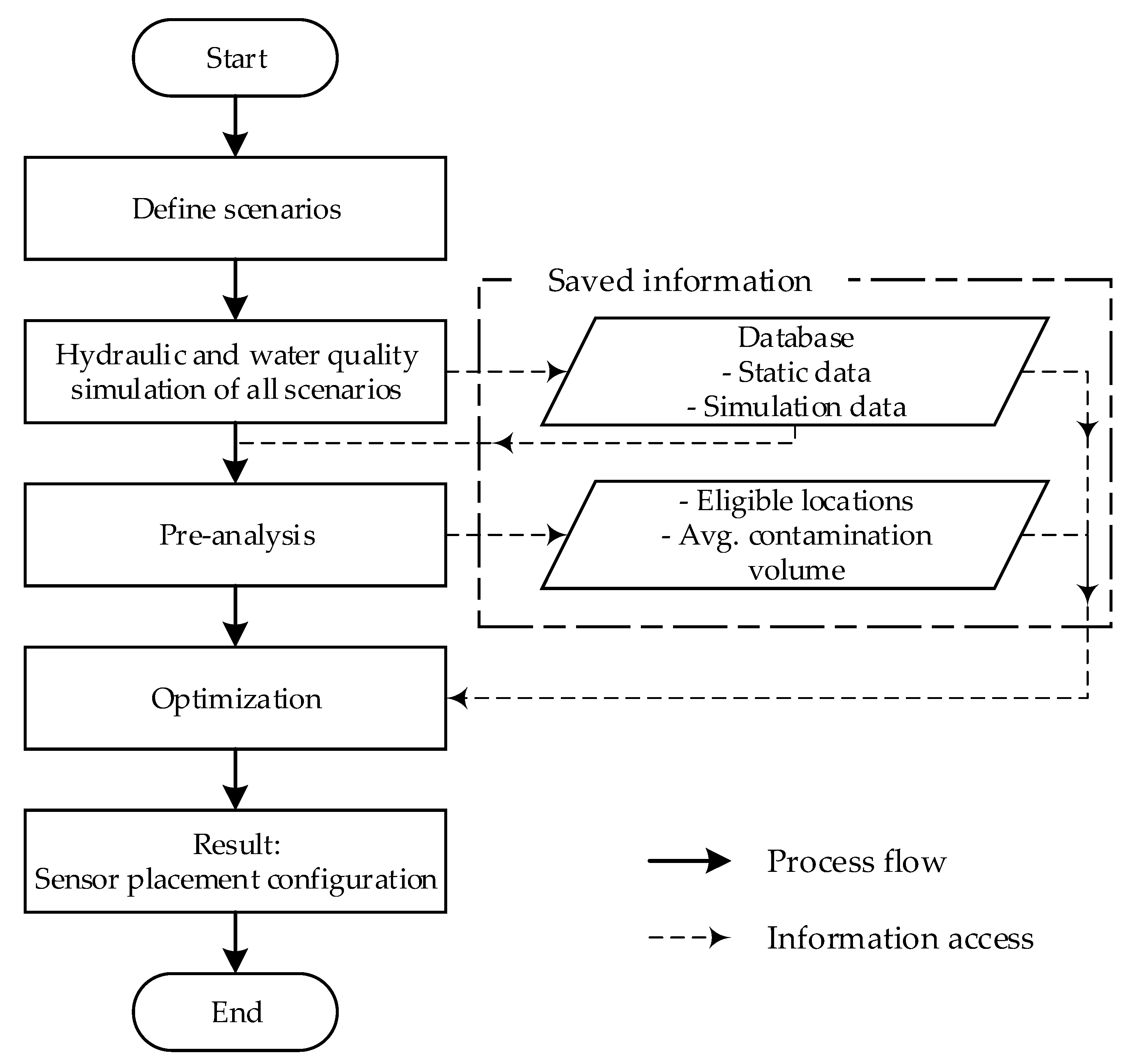
The SPSO method performs SPS optimization using the PSO as the optimization algorithm. As the name suggests, the particle or decision variable of the algorithm is the sensor placement configuration (location of sensors in the WDN). The method aims to provide the best sensor placement based on network data and defined contamination scenarios. The overall process of this method is presented in Figure 1.
The first step in the method is to define the contamination scenarios, which are a combination of the location and time of contaminant injection. Next, hydraulic and water quality simulations are conducted for each scenario, where the result of each scenario is saved to a database. After the simulation is completed, a pre-analysis based on the data is conducted to identify the eligible locations for sensor placement and average contamination volume. Eligible locations can be determined based on the degree of nodes (DoN) or other defined characteristics to reduce the search space. The average contamination volume is the value that is used during the optimization fitness evaluation. Finally, the optimization process is carried out using the database and pre-analysis results.
2.1. Scenario Creation
The optimal SPS should perform well in all potential contamination scenarios. The scenario described here was generated from a combination of multiple intrusion locations and times. Thus, the total number of scenarios is the multiplication of the possible intrusion point (i.e., junction node) and intrusion time (i.e., 24 h). The minimum number of scenarios would be equal to the number of junctions if only one time was considered a critical injection time. Even at the same node, if the injection time is different, it could result in different pathways due to changing water usage with respect to time of day. Therefore, it was better to consider various injection times throughout the day, such as every hour. The injection aftermath can then be observed for each scenario. The contaminant movement through the network over time is especially important. It should be noted that the scenarios are not tied to a specific contaminant, and the sensors are treated as Boolean. Hence, the contaminant concentration is not considered in this study. Therefore, the contaminant is simulated as non-decaying to only account for the presence of a contaminant in the system.
2.2. Databasing
During the optimization process, the defined scenarios were tested using the sensor set solution. As hydraulic and water quality simulations are complicated calculations, testing each solution while performing simulations will consume a significant amount of computational power and time. To combat this resource hogging, a databasing method was applied. This databasing method utilizes a set of predefined scenarios instead of performing a stochastic analysis. The database stores all the data from each hydraulic and quality simulation scenario, thus removing the need to access the network file and simulate every possible solution.
One of the essential databases is the static network database, wherein the data were fixed and did not change over time. In this database, the characteristics of the network nodes and links were stored. The data of the node contain the id, type, base demand, and coordinates, whilst the data of the link include the id, type, length, diameter, and connected nodes. The other database is the simulation database, where the simulation results are stored. Two simulation databases were created. The first was used to store the demand at each node during the simulation. This database is fixed regardless of the scenario because the water consumption will be the same. The second was created for every scenario and contained information needed to determine the contaminant spread behavior, which can be reflected through the contamination status of all the nodes through the simulation time. This database stored the time and status matrices of all scenarios (TS matrix). An example of a TS matrix is presented in Table 1. The rows denote the time in seconds, the columns denote the node, and the cells show the contamination status (1 for true and 0 for false).
As shown in Table 1, in this scenario, the contaminant source can be identified by the earliest detected contaminant, which is Node 1 at time 0. The contamination spread sequence can be derived by observing the status of each node over time. After the contaminant is injected at Node 1, it then spreads in sequence from Node 3 to Node 2 and finally Node 5. Coincidently, Node 4 is free from contaminants. We can then use these databases to check how the sensor responds when placed at a specific location during optimization. For example, considering only a single sensor, it detects a contaminant immediately if it is placed at Node 1. However, placing the sensor at Node 4 will result in no detection of contaminants. It can be said that for this specific scenario, placing the sensor at Node 1 produces the best result. However, more scenarios need to be considered, demanding optimization to achieve a balanced result.
2.3. Optimization
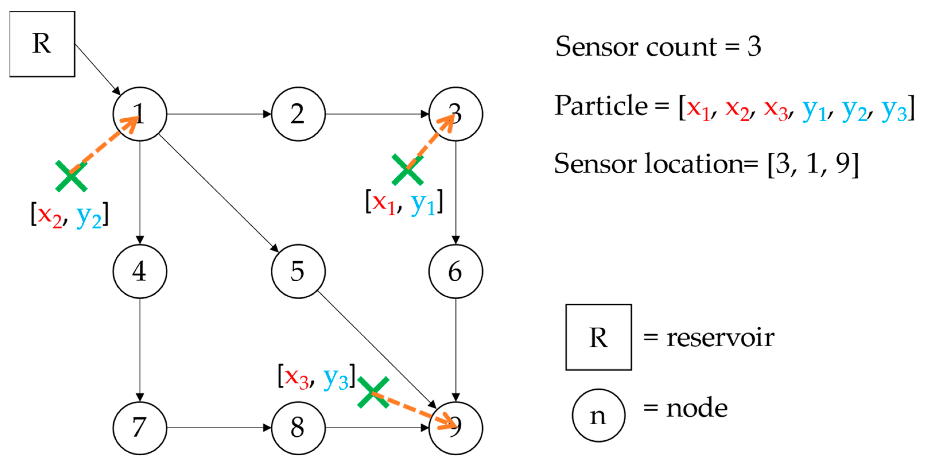
Unlike the conventional SPS optimization approach, where the decision variables are usually the status of the nodes as sensors, a map-based optimization was conducted in this study. The decision variables in this calculation were the coordinates of the search points that determine the nearest node location in the network map. By this definition, to describe the abscissa and ordinate of a sensor in a single vector, the number of decision variables was twice the number of deployed sensors. An illustration of this method is presented in Figure 2.
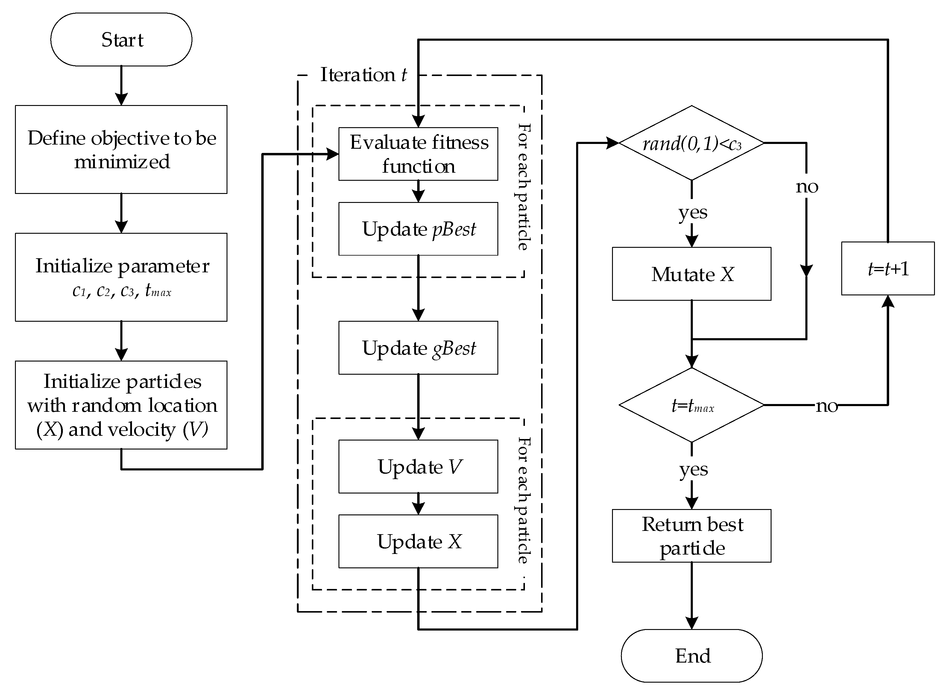
PSO is a meta-heuristic algorithm that can be used for discrete, continuous, and combinatorial optimization problems. The algorithm takes inspiration from swarms’ social behavior in nature, such as bird flocking or fish schooling [18]. The swarm explores the search space to reach an unknown destination (fitness function). Each individual in the swarm is a candidate solution and is referred to as a particle. The algorithm starts by initiating random particles in the swarm where each particle has knowledge of its velocity, the best-achieved location in the past (), and which particle is currently the global best inside the swarm (). At every iteration step, each particle will try to move to a location that is closer to both and by adjusting its velocity. In this study, a modification was applied to the PSO algorithm, specifically in the evolution part, where a mutation factor is used. The workflow of the PSO is shown in Figure 3 and explained afterward.
For this problem, each particle represents the coordinate point of each sensor. The vectors contained in each particle are described as follows.
- (1)
- Location
The location vector contains coordinate points. The abscissa is stored in the first half and the ordinate in the second half, where the vector length was . During the algorithm initiation at , this value was generated randomly from the minimum () and the maximum () coordinates of the nodes in the network. Equations (1)–(5) describe the contents of the location vector.
where is the vector length; is the number of sensors; is the maximum of the contained elements; and are the abscissa and ordinate of node , respectively; is the number of junctions in the network; is the particle’s location element at iteration (initialization); is the random uniform numbers drawn between the contained first and second element; and are the minimum and maximum allowable location respectively; is the location vector of the particle at iteration ; is the location element of the particle at iteration .
- (2)
- Velocity
The velocity vector contains the velocity of the particle, which controls the coordinate displacement in the next iteration. At , the velocity was generated randomly from the number between the minimum velocity () and maximum velocity (). The element of the velocity vector is described by Equations (6) and (7).
where is the velocity element of the particle at iteration (initialization); and are the minimum and maximum allowable velocities, respectively; is the velocity vector of the particle at iteration ; is the velocity element of the particle at iteration .
- (3)
- Personal best location ()
The personal best location describes the location at which a particle achieves the best fitness. This vector is empty during , and is updated as the iteration proceeds.
where is the best location vector of the particle, is the personal best location element of the particle.
- (4)
- Global best location ()
In each iteration, the particle with the best fitness value in the swarm was saved as the , as shown in Equation (9).
where is the best location vector of the swarm, is the best global location element of the swarm.
The evolution of the particle was applied by adding a new velocity to the current particle location where the new velocity was affected by the distance between the current location and the personal best location (individual component) and the global best location (social component). In the individual component, the interval of the personal best to the current location was multiplied by the individual learning rate, which was a randomly generated number between 0 and . The social component was the distance between the current location and the known best location in the swarm affected by the social learning rate, which was another randomly generated number between 0 and . Another important element was inertia () [19], which controls the influence of past velocity into a new velocity. The inertia adapts with the increase in iteration by decreasing the past velocity influence to balance the local and global search. Equations (10)–(12) show the evolution calculation.
where is the inertia weight, and are the individual and social acceleration constants, respectively, is the current iteration step, and is the maximum allowable iteration.
One of the reasons why PSO was chosen over the more commonly used GA is that this optimization scheme allows the sensor to be moved with respect to its past position instead of creating a new set of points. This behavior allows for fine adjustments near the current point. However, without some modifications, the algorithm can still get stuck at the local optima. In this study, another variable, , was added as a mutation factor. The variable enables an individual to change some of its elements without considering velocity. The applicability of mutation to a location vector and the mutation procedure are described in Equations (13) and (14):
where is the mutation factor, is the mutation function and is the independent probability for each element to be mutated.
3. Objective Functions
The optimization requires a direction to go to; thus, quantifiable objective functions were necessary to guide it. The objective functions considered in this study include the detection, consumption, and source identification stages of a contamination event, particularly the objectives are blindspot (BS), consumed contamination (CC), and localization efficiency (LE). Each objective was designed to show an improvement in SPS performance as the value decreases. Hence, the target is minimized. The multiple objectives are grouped into a single fitness value by averaging their values, as shown in Equation (15).
where is the fitness value, is the blindspot value, is the consumed contamination value, and is the localization efficiency value. Note that the objective function values range from 0 to 1, as described in more detail in the following sections.
3.1. Blindspot (BS)
The first stage of a contamination event starts with the intrusion of a contaminant into the WDN. The presence of this contaminant was assumed to be undetected until a WQS picked it up and, in the worst case, remained undetected if no WQS detected it. The BS quantifies the sensor configuration capability to detect contamination in various scenarios. The contaminant injection spread to specific locations depending on the scenario injection characteristics. When a sensor was located in any of the pathways, it resulted in a detected scenario. This objective function shows good performance with an increase in detected scenarios or a decrease in undetected scenarios, as defined in Equation (16).
where is the number of undetected scenarios, is the total number of scenarios.
3.2. Consumed Contamination (CC)
After a contaminant enters the WDN, it is in an undetected state until the sensor detects it. In this undetected state, contaminated water was still being consumed inadvertently, endangering user health. It was assumed that the water usage stopped only after detection. Therefore, the purpose of the CC objective was to consider the duration and spread of the contaminants until detection. Several events can occur at different locations and have the same contaminated volume until detection. However, these events were not considered equal in severity as the contamination was not instantly stopped because of potential sensor malfunctioning [20]. Contaminant intrusion at a point with many downstream connections may cause severe consequences because it enables a larger area to be infected. To reflect this, a weighted factor was applied to this objective. The weight was assigned by the possible affected base demand of each scenario, and base demand was used as a surrogate for the network users. A good measurement for this objective was observed if sensors were placed upstream or after high demand nodes to reduce the consumption volume and downstream contamination chance.
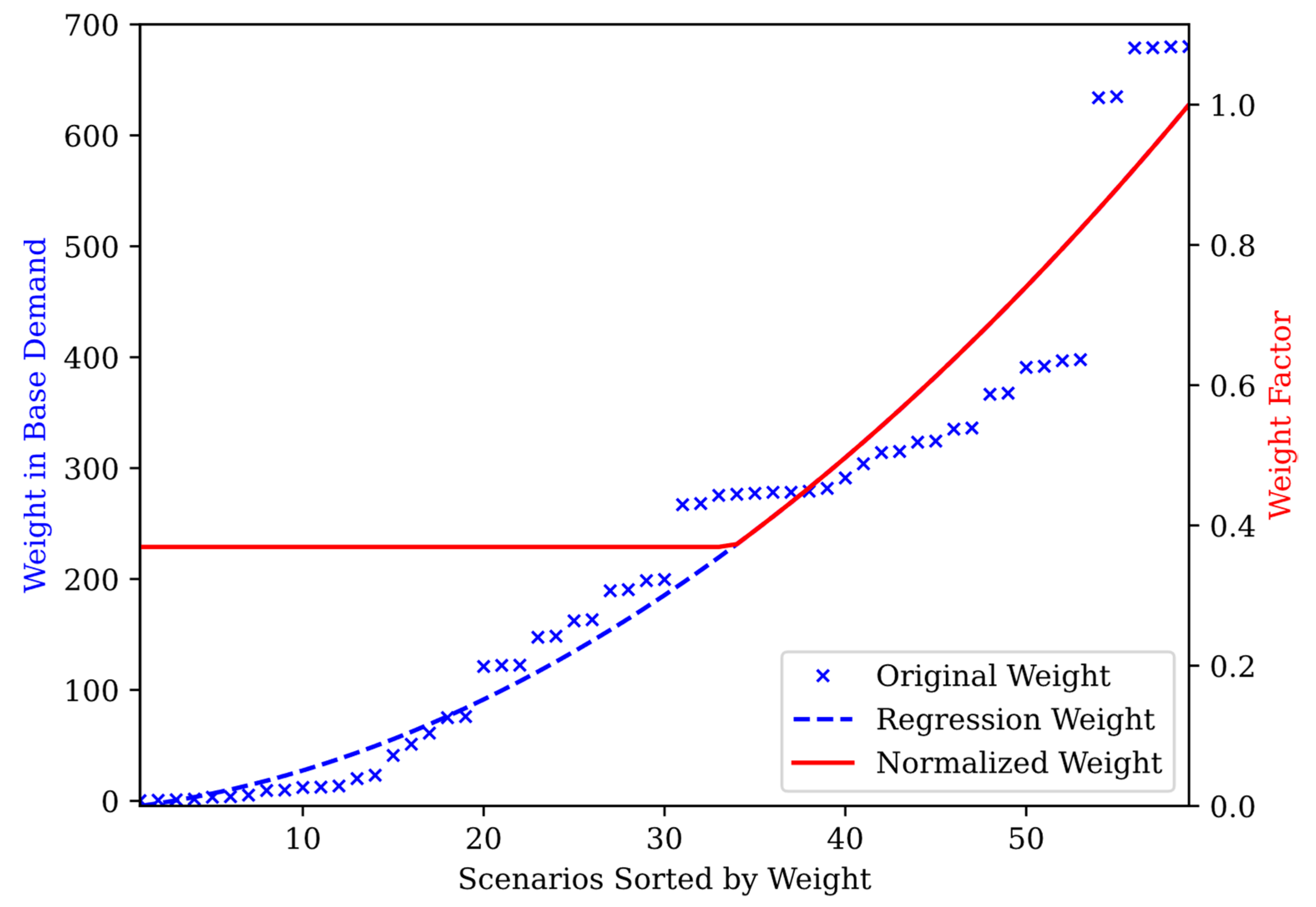
To obtain the CC value, the scenario weight was first calculated. The weight for each scenario was first calculated by observing the possible contaminated area of each injection scenario through the database. Then, the infected base demand of each node was summed as the weight of the scenario, and the weights were sorted in ascending order. A two-degree polynomial regression algorithm was then applied to smooth the weight and prevent large leaps. The weight was then normalized using a min-max normalization to convert it into weight factors. As the values were turned into a range of 0 to 1, multiplication by 0 removed the scenario. Scenario removal was not desired, as a contamination event should not be disregarded, no matter how small. The average weight factor was used as the minimum weight. In the final weight, all values below the minimum weight were changed into the minimum weight value. This prevented scenario removal and underestimation of the scenario. The sorted weights were then redistributed to the related scenarios. A visualization of the weight calculation is shown in Figure 4.
Initially, the contaminated base demand of each scenario was calculated and then sorted in ascending order, as represented by the blue cross mark. The regression was applied, turning it into a dotted blue line. The contaminated base demand was then normalized, and the average value was calculated. The weight factor starts from the average value, as seen in the figure, where the red line starts flat until it intersects with the blue line.
The CC was then calculated after the scenario weight was calculated. For a single scenario, the contaminant will continue to spread until the full saturation time, when all the possible areas are contaminated without any sensor application, is reached. This means that the amount of contaminated water consumed continued to increase exponentially with time, as earlier contaminated nodes still consumed water. The ratio of consumed contaminated water when the sensor was deployed to the non-sensor condition would be distorted. To obtain a more impactful divisor, instead of using the total contaminated volume of all nodes until the full saturation time, average consumption is used. The average consumption is calculated by averaging the total consumption of each node and adding the standard deviation, as shown in Equation (17). This guarantees a smaller divisor that works better during optimization and is still a good representation of the situation.
where is the average consumed contaminated water without sensor deployment during scenario ; is the total consumed contaminated volume until saturation time of node ; is the total number of nodes, and are the average and population standard deviations of the contained elements, respectively.
The CC can then be calculated as in Equation (18).
where associated with scenario , is the weight factor, and is the consumed contaminated water during sensor deployment.
During undetected events, the is equal to . In this way, the effect of an event being undetected can be measured. This action allows the algorithm to choose which cases of undetected event are safer (with lower weight) when it is not possible to detect all events.
3.3. Localization Efficiency (LE)
In the mitigation process of a contamination event, the critical step is to find the contamination source after the sensing period [21]. This objective function describes the amount of information available for the source localization step. As more sensors are able to detect contamination, there will be an increase in accuracy for detecting the source [22]. The LE value is better when the contamination event is picked up by multiple sensors, as expressed in Equation (19). To improve this objective, sensors are more likely to be deployed downstream. This value only applies to detected contamination events, so it does not account for undetected events such as the BS value.
where is the number of sensors detecting the contamination during scenario ; is the number of sensors deployed in the network, and is the number of detected scenarios.
4. Application
In this study, simulations were conducted using the Python 3 programming language [23] and was supported by the Water Network Tool for Resilience (WNTR) 0.3.0 Python package [24] to utilize the EPANET hydraulic simulation model. The databases were created using MySQL and connected to Python, which was able to take advantage of multiple CPUs, whilst the calculation scheme allowed for parallel computing.
4.1. Study Networks
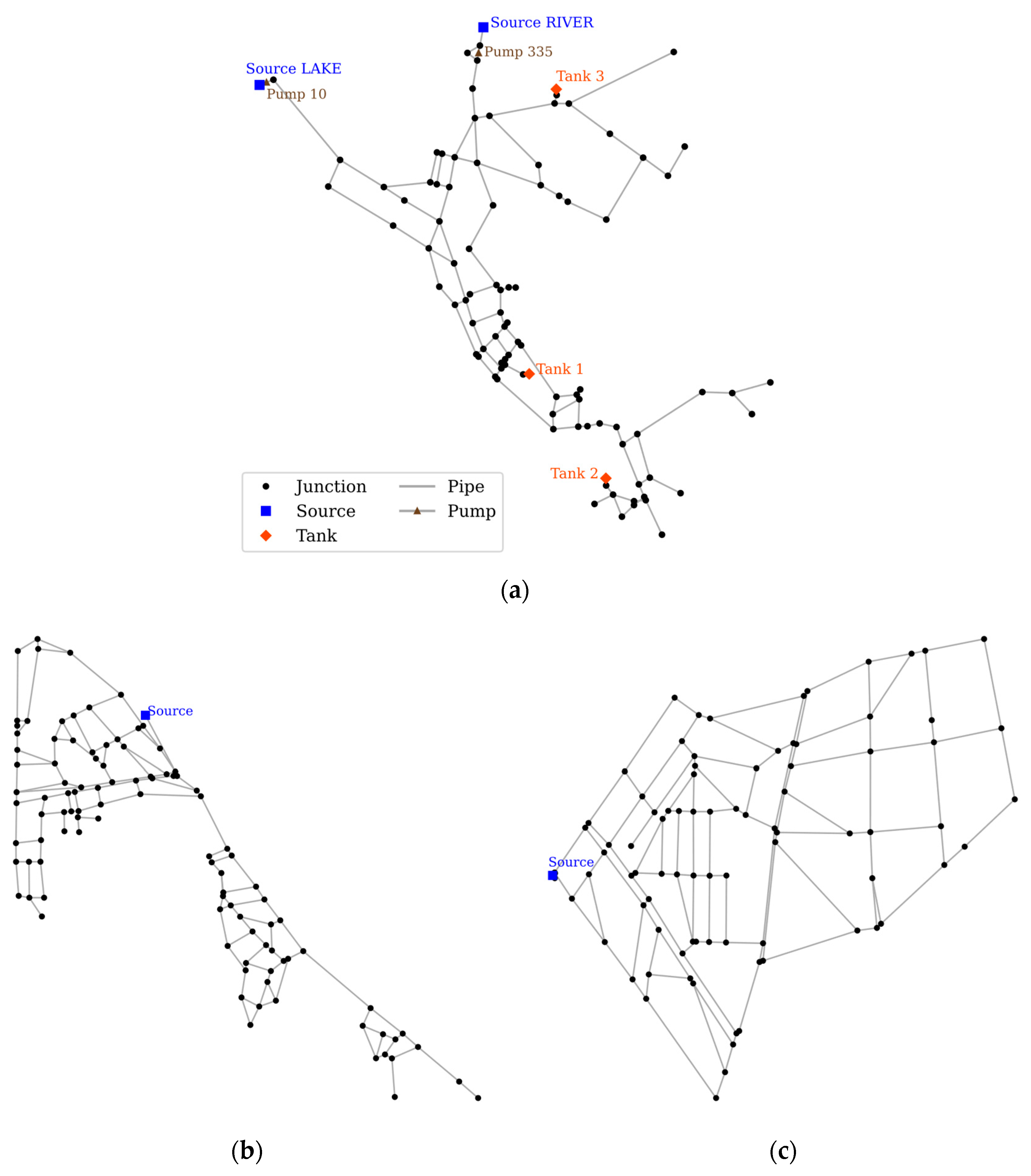
Three networks were utilized in this study. The first network was the well-known EPANET example network 3 (NET3). This network is used as a benchmark for the SPS performance by comparing it with the sensor placement of the example in the threat ensemble vulnerability assessment and sensor placement optimization tool (TEVA-SPOT) [25]. The second and third networks were real DMA-sized WDNs operating in South Korea. These networks were used to show the behavior and performance of the SPSO with an increase in the number of sensors. The layout and details of the networks are shown in Figure 5 and Table 2.
4.2. Benchmark Comparison (NET3 Network)
In the example provided by TEVA-SPOT, the SPS was based on minimizing the extent of contamination, which was the length of the contaminated pipes. Here, it was decided for each junction to have 24 different contaminant injection times with one-hour intervals. The total number of scenarios was 24 multiplied by the number of junctions, totaling 2184 unique scenarios. The hydraulic and water quality simulations were performed, and all the required databases were created. After this, a pre-analysis was performed to determine the weight distribution of each scenario and the average contamination volume. The eligible locations for sensors were limited to only nodes with a DoN of at least three, preventing sensors from being placed at dead-end nodes and serial connections. The evolution parameters for the SPSO are set as .
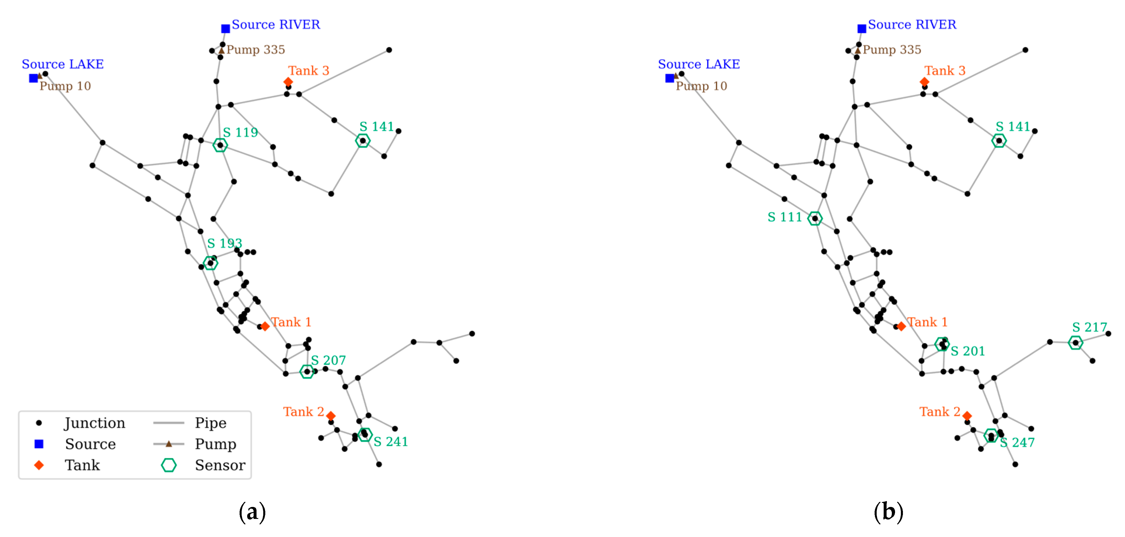
Applying SPSO to NET3, the results show an improvement compared with the TEVA-SPOT example. The sensor placement layout comparison is provided in Figure 6, and the results are summarized in Table 3. Note that the number of deployed sensors is five in both studies.
Results from SPSO show that it performs better than the TEVA-SPOT with all three objective values. Among the five deployed sensors, only one sensor (S 141) is used in both studies. Two sensors have close placements, i.e., S 247 is adjacent to S 241, and S 201 is near S 207. The overall fitness value shows an improvement of 23.1%, resulting from the improvement of all objectives without any trade-off. The BS improved with the addition of S 217, increasing the capability to detect contamination upstream of the location, and the total number of undetected scenarios decreased from 433 to 280. The CC value showed the most significant improvement compared with the other objectives and favors the sensor to be placed upstream or after high-demand nodes. This is reflected by S 111, which was located upstream compared to S 193 in the TEVA-SPOT. Although S 119 was upstream in the TEVA-SPOT, removing it did not degrade the CC value. By inspecting the simulation, it was found that most of the high-demand nodes were located on the left side of the network, meaning that the placement of S 119 was not optimal. The LE also shows improvement by SPSO, as there are more sensors in the downstream area of the network with S 217, which provides additional sensor readings for most contamination events that occurred upstream of it. The reduction of upstream sensors might be harmful in terms of CC, but the new SPS shows that this is not the case.
4.3. SPSO Performance Evaluation (NET-A and NET-B Networks)
The SPSO method performed well for the benchmark network, as shown in the previous section. In this section, the method was applied to configure the SPS in two real-life DMA-scale networks to show how the SPSO performs with an increase in the number of sensors in different types of network characteristics. Note that minimum of three sensors were deployed for both networks because NET-A has three looped-blocks. Same number of sensors was deployed for both networks, which were three (Config-A), four (Config-B), five (Config-C), and six (Config-D) sensors. Sensor locations were limited to only nodes with a DoN of at least three, and the evolution parameters for the SPSO were set as . The same limitations and parameters were applied as previously described.
4.3.1. SPSO Performance on NET-A
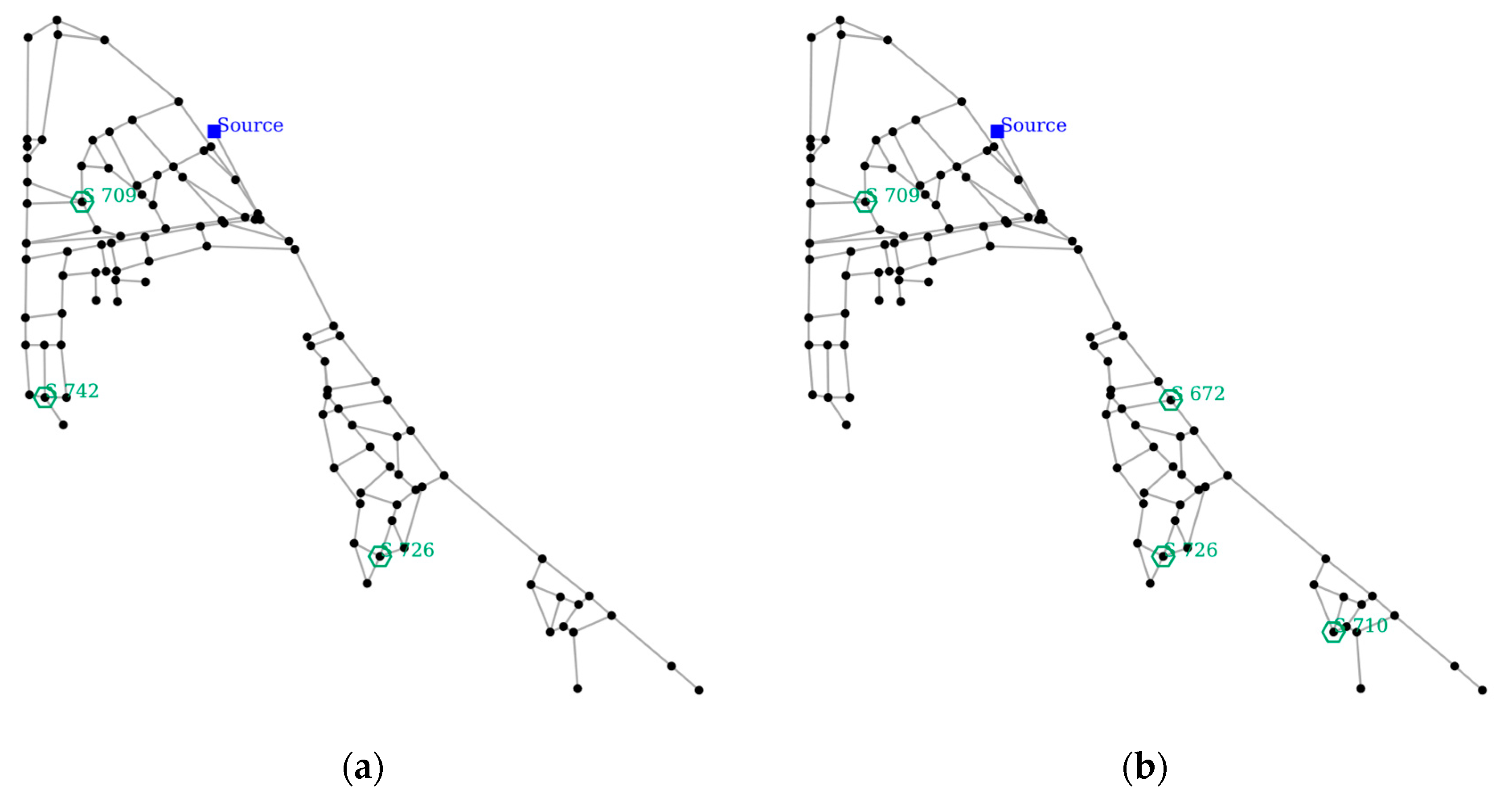
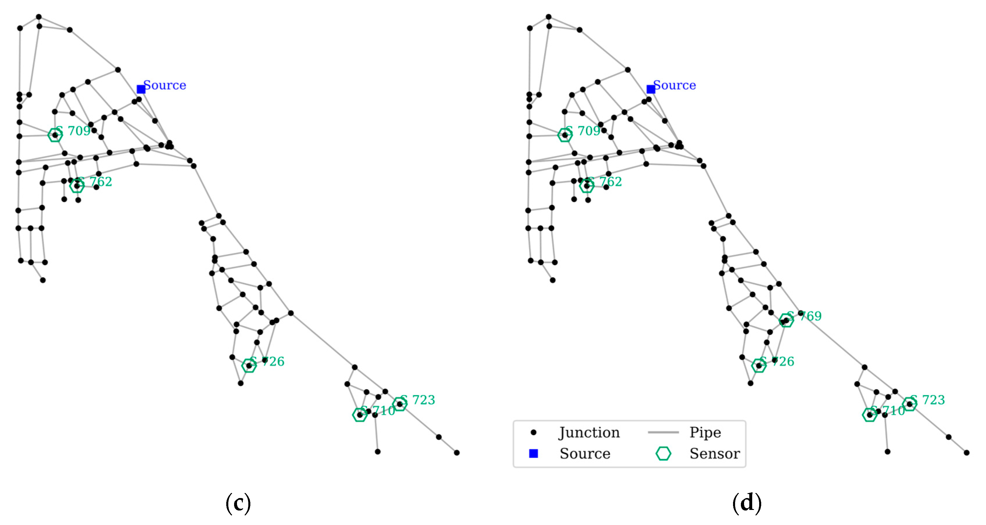
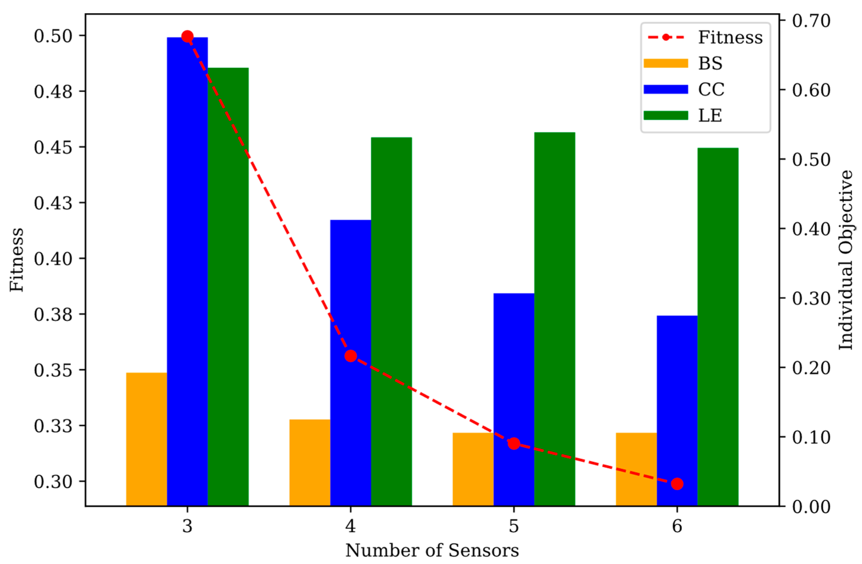
NET-A featured a hybrid branch-looped network in which one source supplied water to the largest looped section, and a bridge connection in series connected two smaller looped sections. SPSO was used to assign three to six sensors in the network. A comparison of each configuration of the sensor is shown in Figure 7. A numerical performance comparison of each configuration is summarized in Table 4, and Figure 8 shows a graphical comparison.
The increase in the number of sensors resulted in an improvement in the fitness value and overall objectives, with a diminishing return of improvement noted by observing the slope of the fitness. The most significant improvement was found when the number of sensors was adjusted to four from three, in which the fitness improved by 0.1434 and CC by 0.2629. Config-A (three sensors) placed two sensors in the large section and one in the medium section, while the small section did not have any sensors placed. This created many undetected events, large consumption of contaminants before detection, and poor localization efficiency. Config-B (four sensors) placed one sensor in each of the large and small sections, whilst two sensors were placed in the medium section. The configuration was found to be more balanced, and a steep improvement in fitness was observed, as shown in Figure 8. The BS and LE for configurations B, C, and D did not change significantly with the LE impaired by a tiny value in Config-C but still exhibited a better fitness value than its predecessor owing to the improvement in CC and BS. The addition of one more sensor in Config-D did not improve the BS, but it did improve the other objectives. In this application, CC showed the greatest improvement with the increase of sensor numbers, followed by BS and LE. Additional sensors reduced the amount of consumed contamination in this hybrid network by providing more cover to the branch section; thus, the LE did not benefit from the dispersed sensor configuration.
The layout figure shows that sensors S 709 and S 726 were always placed, signifying that the location is strategic for sensor placement. Sensor S 710 was also present for all except Config-A and Sensor S 723 for Config-C and Config-D. Config-D placement proved to be a superset of Config-C, as it only added Sensor S 769 as the 6th sensor. This can be explained by observing the objective, particularly in the BS. As there was no improvement in the BS, Config-C minimized the undetected events. An additional sensor was placed to improve the other objectives. Increasing the number of sensors showed that additional sensors were more likely to be placed in the medium and small sections instead of in the large section. Due to the medium section having its water supplied from the large, looped section, any contamination sourcing from the large section would eventually reach the medium section, but not vice-versa. Therefore, placing more sensors in the large section did not benefit the BS and LE. Finally, it featured a balanced placement of the two sensors in each section in Config-D.
4.3.2. SPSO Performance on NET-B
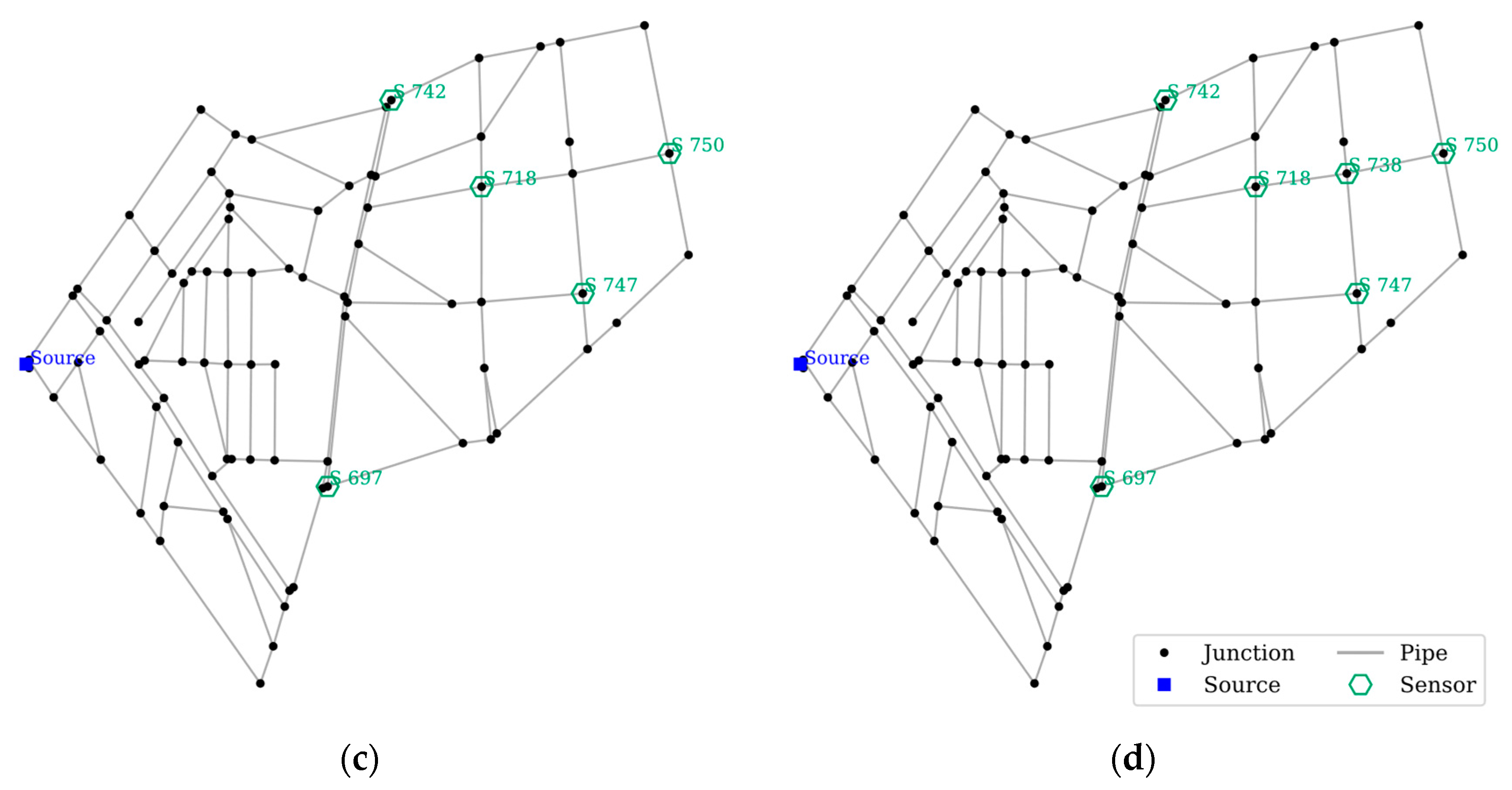
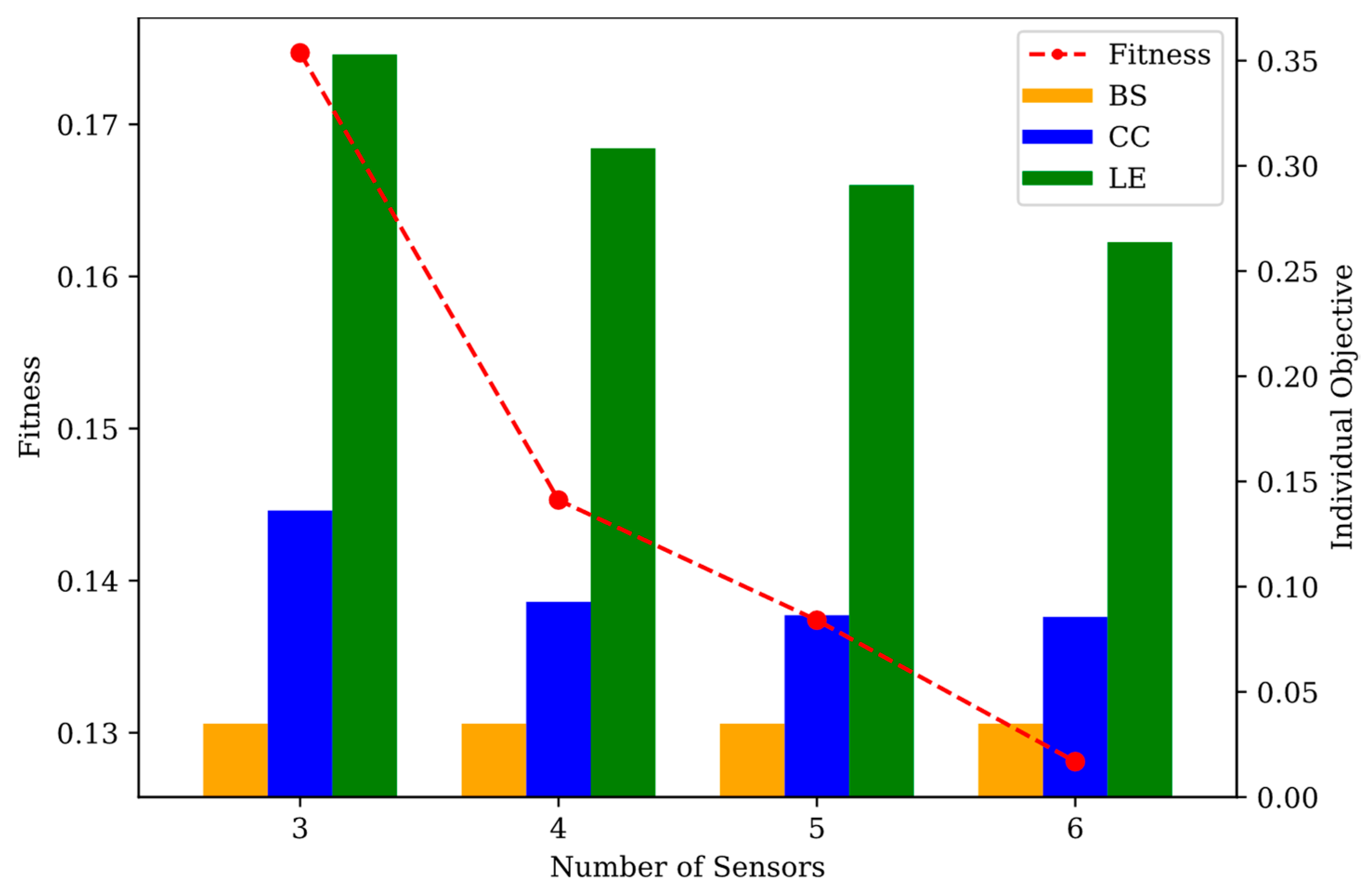
NET-B was a densely looped network that features more high-demand nodes in the east area. Owing to the densely looped nature of the network, most of the flow that reached the east area passed through the majority of the nodes in the west area. In other words, contamination sourcing from the west area was extremely likely to reach the eastern area. The sensor placement layout for each configuration is shown in Figure 9, and the performance comparison is presented in Table 5 and Figure 10.
A low BS of 0.0349 was achieved by placing only three sensors, which translated to 72 out of 2088 scenarios not detected, with the additional sensors only improving the CC and LE. Similar to the application in NET-A, adding more sensors resulted in an improvement of fitness and the objectives individually (except for BS being constant). Using Config-A as the base, the most significant improvement jump was in Config-B, and the subsequent addition of sensors only resulted in a slight improvement of the fitness value. Config-B to Config-D did not show much change in the CC value, while LE continued to improve. It was easier for the configuration to produce a good BS value in a highly looped network because the flow to downstream nodes was received from various upstream nodes. In this case, three sensors proved to be sufficient to detect all contamination events except contamination emanating from dead-end nodes. The CC was also affected by a looped network structure with the same effect, which reduced the number of sensors required to reduce contaminant spread. The detection area of the sensors overlapped, as demonstrated by the diminishing improvement as the number of sensors increased. The overlapping area, in turn, provided more information for localization and improved the LE value instead.
With the east area having more high-demand nodes than the west area, it was preferred to place sensors in the east area. Sensor S 750 was always included, with this node serving as the end node for many sources of contamination. Sensor S 718 was also present for all except Config-A and Sensor S 697 places for all except Config-B. Config-D placement proved to be a superset of Config-C, as it only added Sensor S 738 as the 6th sensor.
Comparing the fitness values between NET-A and NET-B, the overall SPSO performance is better in NET-B. That is, with the same number of sensors placed, a contaminant is more likely to be detected and traced and less likely to be consumed in looped networks compared to branch-type networks.
5. Conclusions
A new SPS method, termed SPSO, which accounted for possible contamination scenarios using PSO, is proposed in this study. SPSO uses objective functions related to the stages of contamination events. The objectives were designed to enhance the ability of the configuration to detect contamination (BS), reduce consumption of contaminated water (CC), and provide information to locate the contamination source (LE). The described objectives were used to evaluate the sensor configuration across possible scenarios of intrusion location and time. Optimization of the configuration uses PSO in map-based optimization to determine the location of the sensor based on the coordinates. Furthermore, a databasing method was also applied to enhance the computation efficiency of the optimization model.
The SPSO was first demonstrated by comparing the configuration result with the TEVA-SPOT example SPS on the well-known benchmark network by applying the same number of sensors. The results revealed that the configuration from SPSO performed better for all applied objectives. The fitness improved by 23.1%, and for individual objectives, the most significant improvement was observed in CC which improved by 35.5%. The benchmark simulation showed that the proposed method is efficient and performs well in locating the sensors. Furthermore, the performance of the method in different network types and number of sensors was analyzed by using two DMA-scale networks. With an increase in the number of sensors, the results showed improved fitness and individual objectives. The increase in fitness experienced a diminishing return, showing that the method can be used to determine the optimal number of sensors to be deployed. It was observed that the BS value had the greatest effect on the placement of sensors, as it was the first to reach the lowest value. This was expected as the detection of the contaminant was the first step that needed to be reached before any action could be taken in practical scenario. The CC value was closely related to the water flow pathways and the nodal demand in the network, with the sensors more likely to be placed near busy pathways and high-demand nodes. The LE had less impact than the other objectives as it modified the sensor configuration to be more optimal after contamination was detected (BS) and after reducing the volume of contaminated water (CC). The results were in line with the expected objective responses to the contamination stages. From the different network characteristics, it was more likely for CC to improve with the addition of sensors in a (loop-branch) hybrid network, whereas in a densely looped network, LE showed more improvement. Comparing the efficiency of sensors, when a similar number of sensors are placed in a network, a contamination event is more likely to be detected and traced, thus inducing less contamination damage in a densely looped network compared to a branch-type network.
The proposed method can be used to determine the strategic locations of WQSs in DMA-sized WDNs. As the method is based on multiple consolidated objectives, users can customize the individual weight of objectives and prioritize some objectives over others. The proposed approach can be further improved by including multiple injection points or by considering the flow uncertainties (due to water consumption change in space and time), as well as specifying the contaminant and sensor type in the scenarios. As the study mainly proposed a framework for an SPS method, some parts of the method, such as the objective functions, can be replaced in future studies. Applying a multi-objective optimization scheme to include the sensor number as decision variables will allow for seeking optimal sensor design. A more complex network could also be considered in future case studies.
Author Contributions
M.S.M. carried out the analysis of the proposed method, model simulations, and drafted the manuscript; D.K. provided the original idea of the study and finalized the manuscript. Both authors have read and agreed to the published version of the manuscript.
Funding
This work was supported by the National Research Foundation of Korea (NRF) grant funded by the Korean government (MSIT—Ministry of Science and ICT), grant number NRF-2020R1A2C2009517.
Institutional Review Board Statement
Not applicable.
Informed Consent Statement
Not applicable.
Data Availability Statement
The data presented in this study are available upon request from the corresponding author. The data are not publicly available because of privacy concerns.
Conflicts of Interest
The authors declare no conflict of interest.
References
- Kirmeyer, G.J.; Martel, K. Pathogen Intrusion into the Distribution System; American Water Works Association: Denver, CO, USA, 2001. [Google Scholar]
- Rasekh, A.; Hassanzadeh, A.; Mulchandani, S.; Modi, S.; Banks, M.K. Smart Water Networks and Cyber Security. J. Water Resour. Plan. Manag. 2016, 142, 01816004. [Google Scholar] [CrossRef]
- Rathi, S.; Gupta, R.S. Sensor Placement Methods for Contamination Detection in Water Distribution Networks: A Review. Procedia Eng. 2014, 89, 181–188. [Google Scholar] [CrossRef] [Green Version]
- Lee, B.H.; Deininger, R.A. Optimal Locations of Monitoring Stations in Water Distribution System. J. Environ. Eng. 1992, 118, 4–16. [Google Scholar] [CrossRef]
- Kumar, A.; Kansal, M.L.; Arora, G. Identification of Monitoring Stations in Water Distribution System. J. Environ. Eng. 1997, 123, 746–752. [Google Scholar] [CrossRef]
- Al-Zahrani, M.A.; Moeid, K. Locating optimum water quality monitoring stations in water distribution system. In Proceedings of the Bridging the Gap: Meeting the World’s Water and Environmental Resources Challenges, Orlando, FL, USA, 20–24 May 2001; pp. 1–9. [Google Scholar] [CrossRef]
- Kessler, A.; Ostfeld, A.; Sinai, G. Detecting Accidental Contaminations in Municipal Water Networks. J. Water Resour. Plan. Manag. 1998, 124, 192–198. [Google Scholar] [CrossRef]
- Berry, J.W.; Fleischer, L.; Hart, W.E.; Phillips, C.A.; Watson, J.-P. Sensor Placement in Municipal Water Networks. J. Water Resour. Plan. Manag. 2005, 131, 237–243. [Google Scholar] [CrossRef] [Green Version]
- Watson, J.-P.; Greenberg, H.J.; Hart, W.E. A Multiple-Objective Analysis of Sensor Placement Optimization in Water Networks. Crit. Transit. Water Environ. Resour. Manag. 2004, 10, 1–10. [Google Scholar] [CrossRef]
- Wu, Z.Y.; Walski, T. Multi-Objective Optimization of Sensor Placement in Water Distribution Systems. In Proceedings of the 8th Annual Water Distribution Systems Analysis Symposium, Cincinnati, OH, USA, 27–30 August 2006; pp. 1–11. [Google Scholar]
- Ostfeld, A.; Salomons, E. Optimal Layout of Early Warning Detection Stations for Water Distribution Systems Security. J. Water Resour. Plan. Manag. 2004, 130, 377–385. [Google Scholar] [CrossRef]
- Rossman, L.A. EPANET 2: Users Manual; National Risk Management Research Laboratory: Cincinnati, OH, USA, 2000.
- Preis, A.; Ostfeld, A. Multiobjective Contaminant Sensor Network Design for Water Distribution Systems. J. Water Resour. Plan. Manag. 2008, 134, 366–377. [Google Scholar] [CrossRef] [Green Version]
- Xu, X.; Lu, Y.; Huang, S.; Xiao, Y.; Wang, W. Incremental Sensor Placement Optimization on Water Network. In Joint European Conference on Machine Learning and Knowledge Discovery in Databases; Springer: Berlin/Heidelberg, Germany, 2013; pp. 467–482. [Google Scholar]
- Montalvo, I.; Izquierdo, J.; Pérez, R.; Tung, M.M. Particle Swarm Optimization applied to the design of water supply systems. Comput. Math. Appl. 2008, 56, 769–776. [Google Scholar] [CrossRef] [Green Version]
- Suribabu, C.R.; Neelakantan, T.R. Design of water distribution networks using particle swarm optimization. Urban Water J. 2006, 3, 111–120. [Google Scholar] [CrossRef]
- Eberhart, R.C.; Shi, Y. Comparison between genetic algorithms and particle swarm optimization. In International Conference on Evolutionary Programming; Springer: Berlin/Heidelberg, Germany, 1998; pp. 611–616. [Google Scholar]
- Kennedy, J.; Eberhart, R. Particle swarm optimization. In Proceedings of the ICNN’95 International Conference on Neural Networks, Perth, WA, Australia, 27 November–1 December 1995; Volume 4, pp. 1942–1948. [Google Scholar]
- Shi, Y.; Eberhart, R. A modified particle swarm optimizer. In Proceedings of the 1998 IEEE International Conference on Evolutionary Computation Proceedings. IEEE World Congress on Computational Intelligence (Cat. No. 98TH8360), Anchorage, AK, USA, 4–9 May 1998; pp. 69–73. [Google Scholar] [CrossRef]
- Bristow, E.C.; Brumbelow, K. Delay between Sensing and Response in Water Contamination Events. J. Infrastruct. Syst. 2006, 12, 87–95. [Google Scholar] [CrossRef] [Green Version]
- Wu, S.; Hrudey, S.; French, S.; Bedford, T.; Soane, E.; Pollard, S. A role for human reliability analysis (HRA) in preventing drinking water incidents and securing safe drinking water. Water Res. 2009, 43, 3227–3238. [Google Scholar] [CrossRef] [PubMed] [Green Version]
- Marlim, M.S.; Kang, D. Identifying Contaminant Intrusion in Water Distribution Networks under Water Flow and Sensor Report Time Uncertainties. Water 2020, 12, 3179. [Google Scholar] [CrossRef]
- van Rossum, G.; Drake, F.L., Jr. Python Reference Manual; Centrum voor Wiskunde en Informatica: Amsterdam, The Netherlands, 1995. [Google Scholar]
- Klise, K.A.; Hart, D.; Moriarty, D.; Bynum, M.L.; Murray, R.; Burkhardt, J.; Haxton, T. Water Network Tool for Resilience (WNTR) User Manual; Sandia National Laboratories: Albuquerque, NM, USA, 2017.
- Berry, J.; Booman, E.; Riesen, L.A.; Hart, W.E.; Phillips, C.A.; Watson, J.P.; Murray, R. User’s Manual: TEVA-SPOT Toolkit 2.4; EPA 600/R-08/041B; National Homeland Security Research Center, US EPA: Washington, DC, USA, 2010.
Figure 1.
Methodology flowchart.

Figure 2.
Example of search point behavior in the network.

Figure 3.
Workflow of PSO algorithm.

Figure 4.
Example of scenario weight.

Figure 5.
Network layout of (a) NET3, (b) NET-A, and (c) NET-B.

Figure 6.
Comparison of five sensor placement between (a) TEVA-SPOT and (b) SPSO.

Figure 7.
Sensor configuration for NET-A (a) Config-A, (b) Config-B, (c) Config-C, and (d) Config-D.
Figure 7.
Sensor configuration for NET-A (a) Config-A, (b) Config-B, (c) Config-C, and (d) Config-D.


Figure 8.
Performance comparison graph for NET-A.

Figure 9.
Sensor configuration for NET-B (a) Config-A, (b) Config-B, (c) Config-C, and (d) Config-D.
Figure 9.
Sensor configuration for NET-B (a) Config-A, (b) Config-B, (c) Config-C, and (d) Config-D.


Figure 10.
Performance comparison graph for NET-B.


Table 1.
Example of time and status matrix (TS matrix) of a scenario.
| Time | Node 1 | Node 2 | Node 3 | Node 4 | Node 5 |
|---|---|---|---|---|---|
| 0 | 1 | 0 | 0 | 0 | 0 |
| 1800 | 1 | 0 | 1 | 0 | 0 |
| 3600 | 1 | 1 | 1 | 0 | 0 |
| 5400 | 1 | 1 | 1 | 0 | 1 |
| 7200 | 1 | 1 | 1 | 0 | 1 |
| 9000 | 1 | 1 | 1 | 0 | 1 |
Table 2.
Network details.
| No. of Elements | Network | ||
|---|---|---|---|
| NET3 | NET-A | NET-B | |
| Junctions | 91 | 104 | 87 |
| Sources | 2 | 1 | 1 |
| Tanks | 3 | 0 | 0 |
| Pipes | 115 | 151 | 129 |
| Pumps | 2 | 0 | 0 |
Table 3.
Comparison of objective values between TEVA-SPOT and SPSO.
| TEVA-SPOT | SPSO | Improvement | |
|---|---|---|---|
| Fitness | 0.2851 | 0.2192 | 23.1% |
| BS | 0.1868 | 0.1648 | 11.8% |
| CC | 0.1984 | 0.1280 | 35.5% |
| LE | 0.4701 | 0.3647 | 22.4% |
Table 4.
Performance comparison for NET-A.
| Objective | Config | Number of Sensors | |||
|---|---|---|---|---|
| A | 3 | B | 4 | C | 5 | D | 6 | |
| Fitness | 0.4996 | 0.3562 | 0.3169 | 0.2988 |
| BS | 0.1923 | 0.1250 | 0.1058 | 0.1058 |
| CC | 0.6752 | 0.4123 | 0.3066 | 0.2745 |
| LE | 0.6314 | 0.5312 | 0.5385 | 0.5160 |
Table 5.
Performance comparison for NET-B.
| Objective | Config | Number of Sensors | |||
|---|---|---|---|---|
| A | 3 | B | 4 | C | 5 | D | 6 | |
| Fitness | 0.1747 | 0.1453 | 0.1374 | 0.1281 |
| BS | 0.0349 | 0.0349 | 0.0349 | 0.0349 |
| CC | 0.1362 | 0.0928 | 0.0864 | 0.0856 |
| LE | 0.3529 | 0.3083 | 0.2909 | 0.2637 |
Publisher’s Note: MDPI stays neutral with regard to jurisdictional claims in published maps and institutional affiliations. |
© 2021 by the authors. Licensee MDPI, Basel, Switzerland. This article is an open access article distributed under the terms and conditions of the Creative Commons Attribution (CC BY) license (https://creativecommons.org/licenses/by/4.0/).
Share and Cite
MDPI and ACS Style
Marlim, M.S.; Kang, D. Optimal Water Quality Sensor Placement by Accounting for Possible Contamination Events in Water Distribution Networks. Water 2021, 13, 1999. https://doi.org/10.3390/w13151999
AMA Style
Marlim MS, Kang D. Optimal Water Quality Sensor Placement by Accounting for Possible Contamination Events in Water Distribution Networks. Water. 2021; 13(15):1999. https://doi.org/10.3390/w13151999
Chicago/Turabian StyleMarlim, Malvin S., and Doosun Kang. 2021. "Optimal Water Quality Sensor Placement by Accounting for Possible Contamination Events in Water Distribution Networks" Water 13, no. 15: 1999. https://doi.org/10.3390/w13151999
Note that from the first issue of 2016, this journal uses article numbers instead of page numbers. See further details here.