Assessing Soil Loss by Water Erosion in a Typical Mediterranean Ecosystem of Northern Greece under Current and Future Rainfall Erosivity

Abstract

Soil is a non-renewable resource essential for life existence. During the last decades it has been threatened by accelerating erosion with negative consequences for the environment and the economy. The aim of the current study was to assess soil loss changes in a typical Mediterranean ecosystem of Northern Greece, under climate change. To this end, freely available geospatial data was collected and processed using open-source software package. The widespread RUSLE empirical erosion model was applied to estimate soil loss. Current and future rainfall erosivity were derived from a national scale study considering average weather conditions and RCMs outputs for the medium Representative Concentration Pathway scenario (RCP4.5). Results showed that average rainfall erosivity (R-Factor) was 508.85 MJ mm ha h⁻¹ y⁻¹ while the K-factor ranged from 0.0008 to 0.05 t ha h ha⁻¹ MJ⁻¹ mm⁻¹ and LS-factor reached 60.51. Respectively, C-factor ranged from 0.01 to 0.91 and P-factor ranged from 0.42 to 1. The estimated potential soil loss rates will remain stable for the near future period (2021–2050), while an increase of approximately 9% is expected by the end of the 21th century (2071–2100). The results suggest that appropriate erosion mitigation strategies should be applied to reduce erosion risk. Subsequently, appropriate mitigation measures per Land Use/Land Cover (LULC) categories are proposed. It is worth noting that the proposed methodology has a high degree of transferability as it is based on open-source data.

1. Introduction

Soil loss by water erosion is considered to be a major threat to the soil, with negative impacts on ecosystem services, crop production, water resources, carbon stock and biodiversity [1,2,3,4,5]. Soil formation is an extremely slow process, classified as a non-renewable resources. To this end, it is considered by the European Union as a challenge to be addressed and has become part of the environmental agenda [6,7]. The United Nations Sustainable Development Goals (SDGs) recognize the importance of soil resources for sustainable development and promote their protection to achieve the ambitious goal of zero land degradation by 2030 [8]. In this framework, the Common Agricultural Policy (CAP) supports policies and practices to reduce soil erosion.

In particular, the Mediterranean basin has been characterized as an erosion prone area. It is well-known that both natural and human-induced landscape changes may have profound effects on soil loss [9]. The natural factors include complex topography and steep slopes [10], the uneven temporal distribution of rainfall with the high erosivity [11,12,13] and soil type and texture [14]. The main anthropogenic factors of soil erosion are considered to be the intensive ploughing [15], unsuitable agricultural practices [16], combined with deforestation [9,17] and overgrazing [18,19]. Moreover, recent Mediterranean studies have reported accelerated soil loss rate following wildfires [20,21,22], which have been an integral part of the Mediterranean ecosystem.

Therefore, the large-scale quantitative assessment of soil loss rate is an essential priority for policy making and sustainability. The monitoring of soil loss with field observation and measurements is the most accurate approach [23,24]. However, this is not financially feasible as it is a time-consuming process that requires increased human and technical resources [25]. Additionally, the experimental plots cannot cover large-scale areas, but are limited to defined sites within the watersheds, while systematic measurements are performed over a short period of time [26,27]. The results are thus representative on local scale.

The effective modeling of soil erosion is challenging and has raised concern among the scientific community. The results have improved and can be better used in the policy cycle [28]. The application of the models can improve the identification of vulnerable to erosion areas and susceptibility mapping [29,30]. The results contribute to the watersheds prioritization and implementation of the appropriate mitigation measures to combat erosion [31,32]. In this frame, the Global Soil Partnership (GSP) Plenary Assembly supports that the new UN global soil erosion map will be based on modeling, unlike the previous assessments based on expert judgments.

The literature on the development of soil loss estimation models and their dynamics is long over the past decades. These models use mathematical equations to determine the relationship between different type of factors and erosion process. They classified on different spatial/temporal scales and various levels of complexity [33]. The main factors affecting soil loss rate are the climate, soil characteristics, topography, land cover and vegetation type. In general, the models are categorized as empirical, conceptual and physically-based depending on the physical processes simulated by the model, the algorithms describing these processes and the data dependence [34].

Empirical models are widely applied, especially in data scarce environment as their simplicity requires limited data and parameters. The most well-known empirical models are USLE [35], RUSLE [36], RMMF [37], and EPM [38]. The physical-based models are based on knowledge of the basic processes within the laws of conservation of mass and energy, as well as on the physical understanding of the processes involved in the phenomenon. These include ANSWERS [39], CREAMS [40], KINEROS2 [41], EUROSEM [42], EPIC [43], WEPP [44] and PESERA [45]. In terms of conceptual models, these are based on a combination of physical-based and empirical models and the most common are the AGNPS [46], LASCAM [47] and SWAT [48].

The most commonly used empirical erosion model is USLE [35] and the revised version RUSLE [36]. It should be noted that these models estimate average annual sheet and rill erosion, but not gully erosion. The main advantages of the USLE/RUSLE model are the flexibility, the accessibility of data and the extensive literature review on the adaptability of the method in almost every kind of conditions and environment [49]. This is also confirmed by the fact that has been frequently used at large scale [28,49,50]. Nowadays, the well-established use of Geographic Information System (GIS), Remote Sensing (RS) and Earth Observation (EO) data has increased the efficiency and accuracy of erosion model [9,22,51,52,53,54].

The erosive force of rainfall is expressed as rainfall erosivity and is the main driver of soil erosion. Rainfall erosivity considers the amount and the intensity of rainfall and is most commonly expressed as the R-factor in RUSLE model [55]. The exposure of the Earth’s surface to aggressive rainfall is a key factor controlling the soil loss by water in terrestrial ecosystems and other hydrological hazards [56]. The dynamic nature of the rainfall erosivity (R) factor in RUSLE model [52] makes it suitable for applications under changing climate conditions [57,58,59]. This is highly important as the Mediterranean basin is considered a hotspot for a climate change and biodiversity and is expected to face increased challenges due to climate shifts [60,61]. Although the climate will become warmer and drier, more often, intense precipitation events are expected in the eastern Mediterranean [62] and an increase in the rainfall erosivity [12,63].

The main object of the current study is to evaluate the soil loss in a typical Mediterranean ecosystem (North Greece) under current and future rainfall erosivity conditions based on data from high-resolution regional climate models (RCMs).

2. Materials and Methods

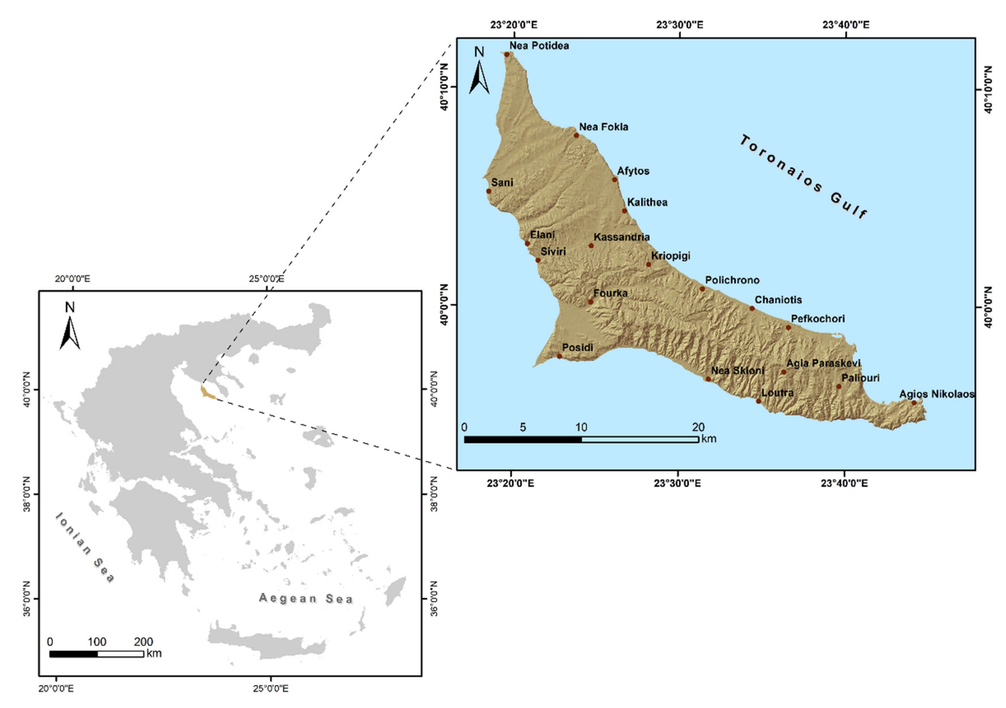
2.1. Study Area

The study was conducted in the Kassandra Peninsula and it is located in Northern Greece (Figure 1). It is a well-known tourist destination with a 350 km² area. The dominant forest species is Aleppo pine (Pinus halepensis), while the presence of shrubland is significant, even in the overstory within the stands [64]. Another characteristic of the landscape fragmentation is the small patches of forest land alternated with olive groves and grasslands.

The climate is typical thermo-Mediterranean and characterized by mild wet winters and dry warm summers. According to the climatic classification of Köppen [65], the study area belongs to the Csa climatic type, which prevails almost all over Greece. The mean annual rainfall is about 600 mm, while the mean temperature is about 16 °C and the pre-long dry period is particularly extended from May to September.

In relation to the geomorphological characteristics, the elevation ranges from sea level to 340 m. The complex terrain and moderate slopes also stand out in the landscape, but the slopes are more intense in the northwest. Degraded from erosion sandy and sandy-clay types of soils predominate in the area and the dominant bedrock is marls (sedimentary rock).

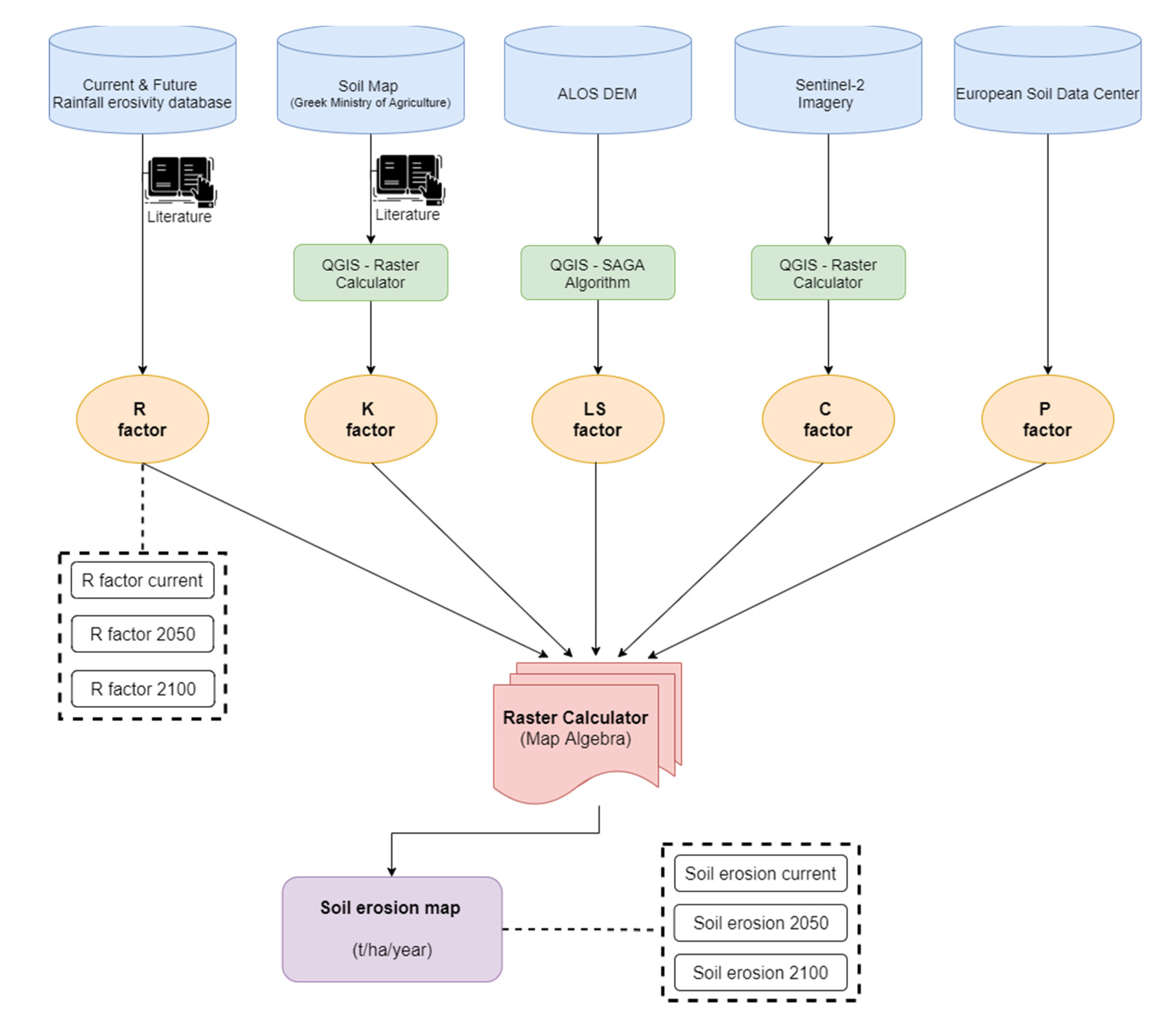
2.2. Soil Loss Modeling and Datasets

The RUSLE model, as indicated by its name, is an updated version of the USLE model. The model computes the mean annual soil loss from sheet and rill erosion as a linear combination of five factors [36],

$$A=R\times K\times LS\times C\times P$$

(1)

where A is the computed annual soil loss (t ha⁻¹ y⁻¹), R is the rainfall erosivity factor (MJ mm ha h⁻¹ y⁻¹), K is the soil erodibility (t ha h ha⁻¹ MJ⁻¹ mm⁻¹), LS is the combined effect of slope length (L) and slope steepness factor (S) (dimensionless), C is the cover management factor (dimensionless) and P is the support practice factor (dimensionless). Based on the above-mentioned factors numerous datasets were collected and analyzed.

These datasets included the rainfall, satellite imagery, soil and topographical data. By using the open source Quantum GIS (QGIS) software package, all the datasets were organized in GIS thematic layers. Subsequently, the determination of each factor during the implementation of the soil loss model is described in the following sub-subsection. A brief flowchart of the methodology and an associated table with the input datasets are presented in Figure 2 and

Table 1. Summary of the input datasets and sources used for the estimation of soil loss in RUSLE model.

Factors	Datasets	Data Source	Spatial Resolution	Format
Current/Future Rainfall erosivity (R)	National Scale Study [66]	https://zenodo.org/record/3692645 (accessed on 1 May 2021) https://zenodo.org/record/3855604 (accessed on 1 May 2021)	~1 km	Raster
Soil erodibility (K)	Soil Map of the Greek Ministry of Agriculture	http://mapsportal.ypen.gr/maps/289 (accessed on 1 May 2021)	-	Vector
Slope Length and Steepness (LS)	ALOS DEM	https://www.eorc.jaxa.jp/ALOS/en/aw3d30/index.htm (accessed on 1 May 2021)	30 m	Raster
Cover management (C)	Sentinel-2—Level 2A imagery	“Copernicus” program https://scihub.copernicus.eu (accessed on 1 May 2021)	10 m	Raster
Support practice (P)	European Soil Data Center	https://esdac.jrc.ec.europa.eu/content/support-practices-factor-p-factor-eu (accessed on 1 May 2021)	1 km2	Raster

, respectively.

The soil loss values were grouped into five erosion hazard classes ranging from very low to very high. The limits of these classes were obtained as described in the national scale studies of Flood Risk Management Plans (FRMPs), conducted in the frame of EU Directive on floods (2007/60/EC).

2.2.1. Rainfall Erosivity Factor (R)

Rainfall is considered as a triggering factor for soil loss. It is a dynamic factor and presents high spatial and temporal variability. It is defined as the average annual sum of the kinetic energy of storm events with, maximum, 30-min rainfall intensity. Unfortunately, rain gauge station data and especially pluviographs are rarely available in eastern Mediterranean and especially the Greece territory. To this end, many simplified mathematical equations managed to link the rainfall erosivity to annual or monthly rainfall data [9,20,67,68].

The values of the R factor were obtained from a national scale study considering average weather conditions [66]. Annual rainfall erosivity was calculated using daily and monthly precipitation records from rain gauge station spatially distributed through Greece. In the above-mentioned study [66] the event erosivity EI₃₀ (MJ mm ha⁻¹ h⁻¹) was computed using pluviograph records and defined as:

$$E{I}_{30}=\left({\displaystyle \sum _{r=1}^m{e}_r{v}_r}\right)\times I_{30}$$

(2)

where e_r is the kinetic energy of unit rainfall (MJ ha⁻¹mm⁻¹) and v_r is the rainfall depth (mm) for the hyetograph’s time interval r, which has been divided into r = 1, 2, …, s time sub-intervals and I₃₀ is the maximum rainfall intensity for a 30-min period during the rainfall.

The unit rainfall energy (e_r) was calculated for each time interval as follows:

$$e_r=0.29\left(1-0.72e^{-0.82i_r}\right)$$

(3)

where i_r is the rainfall intensity during the time interval (mm h⁻¹).

Following the calculation of EI₃₀ values, the average monthly rainfall erosivity density ED_m (MJ ha⁻¹ h⁻¹) per station was calculated:

$${ED}_m=\frac{1}{n}{\sum }_{i=1}^n{\left(\frac{{\sum }_{k=1}^{{st}_m}{\left({EI}_{30}\right)}_k}{P_m}\right)}_i$$

(4)

where st_m is the number of storms during the month m, (EI₃₀)_k the erosivity of storm k, P_m the monthly precipitation height and n the number of years.

Also, in order to create the aforementioned product, the Quantile Regression Forests (QRF) algorithm was used [69] for the spatial mapping of the results. The raster product is available online at: https://zenodo.org/record/3692645 (accessed on 1 May 2021). Noteworthy, previous studies on R in Greece [70] revealed that the reported R values were underestimated due to the presence of a significant amount of missing data in the precipitation records used in the calculations.

Furthermore, the effect of climate change on soil loss was assessed. Hence, future rainfall erosivity was used to address this issue. The future rainfall erosivity raster was likewise produced in the already referenced national scale study [54]. The future projection of precipitation was obtained from Regional Climate Models (RCM) with a fine resolution (10 × 10 km) developed in the frame of the EURO-CORDEX project [57,71] and found that the precipitation condition performs better for a historical time period. In order to evaluate model’s performance comparison between station data and RCMs projections was achieved for the historical period 1971–2000. Statistical indexes, such as root mean square error (RMSE) coefficient of determination R² and Lin’s Concordance Correlation Coefficient (CCC) were used in order to evaluate the model’s performance.

The results demonstrated that the RACMO2 model achieved better performance. This model used later on for the creation of rainfall erosivity raster for current and future conditions. The RACMO2 model developed by the KNMI institute and driven by the General Climate Model (GCM) named EC-Earth. Herein, two scenarios of future R values were evaluated based on the medium Representative Concentration Pathway RCP4.5 scenario, for the near future period (2021–2050) and far future period (2071–2100), respectively.

2.2.2. Soil Erodibility Factor (K)

The soil erodibility factor describes the susceptibility of soil types to detachment and transport as a result of the raindrop and runoff process. It depends on many soil properties, such as soil texture, permeability, shear strength, organic matter and chemical composition [14]. The estimation of the K factor based on field measurements is a complicated and time-consuming process, usually infeasible in large scale studies. Consequently, a reliable methodology in a form of nomograph [72] for the determination of the K values has been developed. The nomograph firstly considering five soil parameters (silt, sand, clay and organic matter content, a soil structure index and soil permeability index) whereas later on was modified in order to account for the rock fragment cover effect [35]. The lower values of K indicate soils less prone to erosion. On the other hand, the higher values attribute to soil susceptible to erosion.

The estimation of the K factor values was based on 1:50,000 scale soil map, from the Greek Ministry of Agriculture. Particularly, the appropriate values were assigned to each parent material according to the relative literature [73,74] and presented in the following table (

Table 2. Soil parent material and assigned soil erodibility (K) values.

Parent Material	K Value
Alluvial Deposits	0.015
Hard Limestone	0.0008
Peridotite	0.05
Tertiary deposits	0.015

).

2.2.3. Topographic Factor (LS)

The slope length (L) and slope steepness factor (S) are commonly combined as the topographic LS factor. The S-factor measures the effect of slope steepness, and the L-factor defines the impact of slope length. The combined LS-factor describes the effect of topography on soil erosion process. The higher values of LS-factor represent steeper relief, where erosion and sediment yield increase due to an increase of the runoff.

The S factor is calculated, according the slope gradient, in degrees ($\vartheta$) as follows [75]:

$$S=\{\begin{array}{ll}10.8\times \sin \vartheta +0.03& \vartheta <0.09\\ 16.8\times \sin \vartheta -0.5& \vartheta >0.09\end{array}$$

(5)

Moreover, the L factor is calculated using the proposed equation by Desmet and Govers [76]. This approach takes into account that the slope steepness is not uniform for the whole area and introduce the concept of the unit-contributing area. The mathematical formula given below:

$$L=\frac{{\left(A_{i,j-in}+D^2\right)}^{m+1}-A_{i,j-in}^{m+1}}{D^{m+2}\times x_{i,j}^m\times {22.13}^m}$$

(6)

where A_i,j,–in is the contributing area (m²) at the inlet of grid pixel (i,j), D is the grid pixel size (m), x_i,j is the summation of the sine and cosine of aspect direction (α_i,j) of grid pixel (x_i,j = sin α_i,j + cos α_i,j), and m is a coefficient related to the ratio b of the rill to inter-rill erosion. Τhe equation for the m coefficient is:

$$m=\frac{\beta }{\beta +1}$$

(7)

$$\beta =\frac{\frac{\sin \vartheta }{0.0896}}{\left[0.56+3\times \left(\sin {\vartheta }^{0.8}\right)\right]}$$

(8)

$\vartheta$ is the angle of slope in degrees and m values varies between 0 to 1. The aforementioned approach [76] demonstrates that this procedure of LS estimation is suitable for landscapes with complex topography.

The LS factor calculation was implemented using the System for Automated Geoscientific Analyses (SAGA) GIS software package which incorporates the multiple flow algorithm [77]. SAGA software offers a robust set of terrain analysis data processing modules [78] and is faster than ArcGIS Toolbox in computing flow accumulation directly from DEMs [79].

A digital elevation model (DEM) is required for the calculation of the LS factor as an input dataset. The Advanced Land Observing Satellite (ALOS) (AW3D30 v.2.2) DEM developed by the Japan Aerospace Exploration Agency (JAXA) with spatial resolution 30 m was selected in this study (https://www.eorc.jaxa.jp/ALOS/en/aw3d30/index.htm, accessed on 1 May 2021). This option is also supported by the literature review concerning its accuracy both in Greece [80,81] and in the Mediterranean Basin [82,83] in comparison with similar products.

2.2.4. Cover Management Factor (C)

Vegetation can significantly protect the surface soil loss and act as a factor to slow down the soil erosion [84]. The normalized difference vegetation index (NDVI) is one of the most widely known satellite-based indicators of vegetation growth and cover [9]. It is expressed by the following computing formula:

$$NDVI=\frac{NIR-Red}{NIR+Red}$$

(9)

where NIR and Red are the near-infrared and red spectrum of a satellite image, respectively.

Using the NDVI image, the C-factor is generated on the basis of vegetation cover, which allows raindrops to subside their kinetic energy before impacting on the soil surface [20]. This cover management factor is expressed as a rate of soil loss under specific conditions such as vegetation and surface coverage.

The C-factor is calculated based on the following equation [84]:

$$C=\exp [-a(\frac{NDVI}{b-NDVI}\left)\right]$$

(10)

where a and b are the parameters that determine the relationship between C and NDVI curve. The a and b are equals 2 and 1, respectively, and are unitless parameters that specify the shape of the aforementioned curve [9,51]. The C Factor ranges between 1 and 0, while closeness to 0 indicates the well protected land.

The C-factor calculation was implemented using the NDVI index of a single-date Sentinel-2A image obtained in the summer of 2020. In particular, the Sentinel-2A Level-2A (launched 31 August 2020) provides high-resolution optical data (10 m, 20 m and 60 m) with atmospheric and radiometric corrections. The image was acquired from the European Space Agency (ESA) Copernicus Access Hub (https://scihub.copernicus.eu) (accessed on 1 May 2021), which provides free access to Sentinel products and processed on GIS software. The spectral bands used in this study were the NIR and Green band of 10 m spatial resolution. As for the mathematical equation of C-factor, it was applied in a QGIS Raster Calculator using the NDVI image and the constant a and b values. Many studies state the profound effect of seasonality on C factor estimation [85]. This occurs due to the rapid change of vegetation conditions during the year. However, the main LULC classes in the study area are permanents (pinewood, olive groove, shrubland) so their canopy characteristics are stable through the year. Therefore, a single-data image acquisition considered representative for the C factor estimation [86].

2.2.5. Support Practice Factor (P)

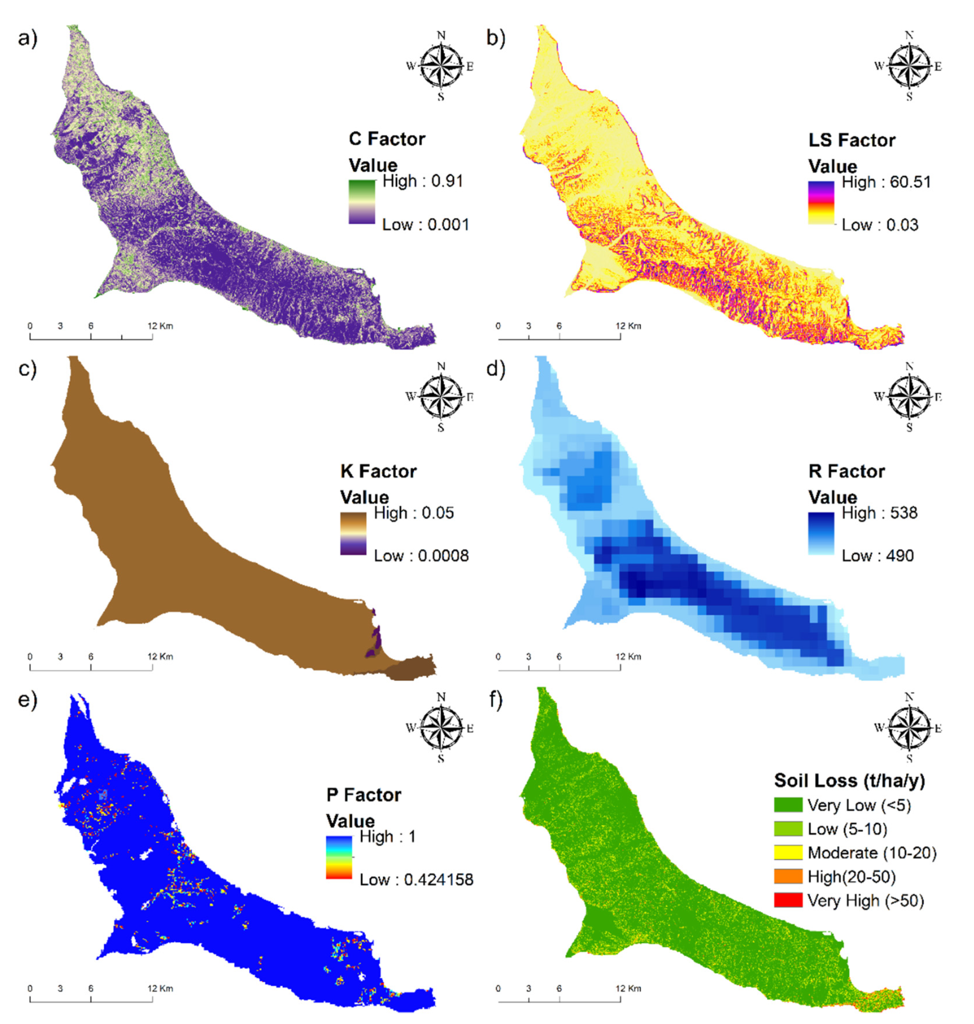
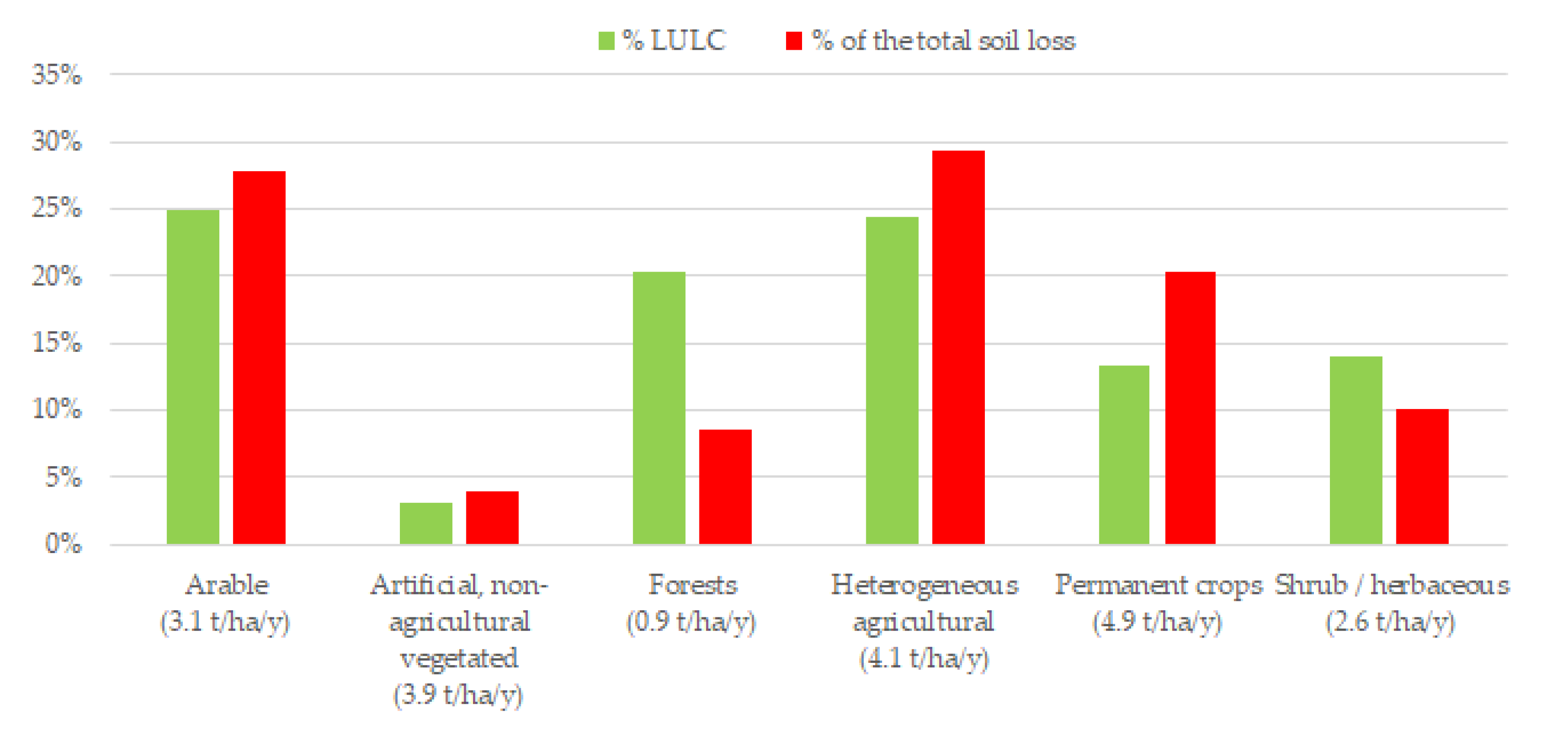
The support practice factor (P) defines the impact of management practices against soil loss. These practices mainly include contour farming, stone walls and grass margins over the examined region. The P values range between 0 and 1. A low P factor, approaching 0, indicates an effective support practice. Whereas, a P factor near to 1 corresponds to the absence of conservation practice.

The P values were obtained in raster format from a recently published study [87] and the associate datasets are available from the European Soil Data Center [88]. In these studies, Greece was included in the list of countries where support practices have the greatest impact.

3. Results

According to the extent of the study area there is no significant spatial variability of the rainfall. The rainfall erosivity (R), as already mentioned in the previous subsections, was derived from a national scale study (see Figure 3d). The rainfall erosivity values ranged from 490 to 538 MJ mm ha h⁻¹ y⁻¹ with a mean value of 508.8 MJ mm ha h⁻¹ y⁻¹ and standard deviation (SD) of 13.3 MJ mm ha h⁻¹ y⁻¹. The spatial distribution of R factor showed a clear distinction between the hilly areas in the central part (with high R value) and the coastal regions (with low R value). The role of topography is emphasized as the mountains are found in the middle part of the study area.

In terms of soil erodibility (K), it must be quoted that the dominant parent rocks were tertiary and alluvial deposits, followed by peridotites and finally smaller area occupied by hard limestones. The soil erodibility values (K) in the study area ranged from 0.0008 to 0.05 t ha h ha⁻¹ MJ⁻¹ mm⁻¹ with a mean value equal to 0.02 t ha h ha⁻¹ MJ⁻¹ mm⁻¹ and standard deviation (SD) of 0.01 t ha h ha⁻¹ MJ⁻¹ mm⁻¹ (see Figure 3c). The topographic factor (LS) values ranged from 0.03 to 60.5, with a mean value of 2.86 and standard deviation (SD) of 2.97 (see Figure 3b). The cover management (C) values ranged from 0.01 to 0.91 with a mean value of 0.22 and standard deviation (SD) of 0.2 (see Figure 3a). The lower values were found in pinewoods, followed by shrublands. In the majority of the study area there is no support practices, as revealed from the European dataset used herein. Therefore, the mean P value is equal to 0.98 and the standard deviation (SD) of 0.07 (see Figure 3e).

The expected potential soil loss (A) expressed in tons per hectare per year (t ha⁻¹ y⁻¹) and was calculated by multiplying the five RUSLE factors. The spatial distribution of the RUSLE factors and soil loss map are presented in the following figure (Figure 3).

The coupling of the above-mentioned factors results to the estimation of soil loss and the creation of the associated map (Figure 3f). The mean annual soil loss was found to be 3.4 t ha⁻¹ y⁻¹, and characterized as very low according the classification categories. The results of the potential soil loss hazard map illustrated that the 80.1% of the study area belong to the very low hazard class, followed by low (13.1%) and moderate (5.1%) hazard classes. Additionally, soil loss characterized as high or very high only in the 1.3% and 0.1% of the area, respectively. Due to a combination of factors, such as steep slopes and barren land, considerable high values of soil loss presented in the coastal zone. This is also common in other Mediterranean coastal areas.

The LULC is the most crucial variable in soil loss models, as it is the only factor that can be altered by humans, for better or for worse. Land Use/Land Cover (LULC) generally refers to the categorization or classification of human activities and natural elements on the landscape within a specific time frame based on established scientific and statistical methods of analysis of appropriate source materials.

Also, it provides an effective erosion control. In order to design an integrated erosion mitigation plan, the identification of soil loss rate per LULC type is required. In the study area, the soil loss was analyzed by LULC based on second level of CORINE (CLC2018) land cover database (Figure 4).

The mean rate of soil loss from arable land is 3.1 t ha⁻¹ y⁻¹. Permanent crops and heterogeneous agricultural areas present higher rates of soils loss than arable lands equal to 4.1 and 4.9 t ha⁻¹ y⁻¹ respectively. This is due the fact that olive trees located in hilly areas and heterogeneous agriculture land in areas with complex relief, while arable lands are in flat or gently sloping areas. The agricultural areas, including arable lands, heterogeneous agricultural areas and permanent crops cover an area of 62.7% of the study area. The rate of soil loss in agricultural areas is 4.1 t ha⁻¹ y⁻¹ and is 20% higher than the overall mean. These agricultural lands account for 77.5% of the total soil losses. As for the artificial, non-agricultural vegetated areas, results covering only the 3.1% of the study area and having a relative low impact on soil loss in the current study. The forests present by far the lowest rate of soil loss (0.9 t ha⁻¹ y⁻¹). Despite covering more than 20% of the area, forestlands contribute to less than 9% of the total soil loss. Finally, areas covered with shrubs and herbaceous vegetation concentrate 14% of the study area and have a mean soil loss above average (2.6 t ha⁻¹ y⁻¹).

In order to evaluate the climate change effect on the potential soil loss, the RUSLE model was applied under future climate conditions, as derived from the RACMO2 RCM. According to the RCP4.5 scenario, the process was carried out for the near future (2021–2050) and the far future period (2071–2100). Spatial difference between the projected R factor and the baseline period (1971–2000) showed an increase of 4.4 MJ mm ha h⁻¹ y⁻¹ and 46.1 MJ mm ha h⁻¹ y⁻¹ for the 2021–2050 and 2071–2100 periods, respectively. As a result, the changes are considered to be higher in the northwestern part of the study area and will intensify until the end of the 21th century (Figure 5).

The aforementioned changes in R factor will also affect the soil loss potential. The outcomes of the RUSLE model implementation under climate change conditions are presented in the following figure (Figure 6). The mean annual soil loss will remain stable until 2050, with a mean difference from the baseline period of 0.02 t ha⁻¹ y⁻¹ and a standard deviation (SD) of 0.12. However, an increase (+8.7%) is expected for the far future period (3.7 t ha⁻¹ y⁻¹) with mean difference from the baseline period equal to 0.31 t ha⁻¹ y⁻¹ and standard deviation (SD) of 0.52. Nevertheless, the hazard classes’ rates remain the same without any notable change for both near future and far future period.

4. Discussion

The soil loss by sheet and rill erosion was estimated using the RUSLE model. Unfortunately, there are no experimental plots in the study area. However, studies in Greek territory comparing model with actual measurements showed acceptable accuracy, despite a slight underestimation approximately equal to 30% [89,90].

The mean annual rate of soil loss due to water erosion in European Union (EU) is estimated equal to 2.46 t ha⁻¹ y⁻¹ [28]. The variety of geomorphological, climatological and land use conditions across EU lead to a wide range of erosion values. As reported by Panagos [28], the highest mean annual soil loss rate (at country level) is found in Italy (8.46 t ha⁻¹ y⁻¹), followed by Slovenia (7.43 t ha⁻¹ y⁻¹) and Austria (7.19 t ha⁻¹ y⁻¹) due to a combination of high rainfall erosivity and complex topography. Particularly, in the Mediterranean countries, including Greece, the mean rates of soil loss are also higher than pan—European average [28,91], as can be seen in the following table (

Table 3. Average soil loss rate in Mediterranean countries.

Country	Averaged Soil Loss (t ha−1 y−1)
Croatia	3.16
Cyprus	2.89
France	2.25
Italy	8.46
Greece	4.13
Malta	6.02
Portugal	2.31
Slovenia	7.43
Spain	3.94

).

This is also confirmed by the findings of the current study, as the mean rates of soil loss in the Kassandra Peninsula (Northern Greece) are estimated equal to 3.4 t ha⁻¹ y⁻¹. It is noteworthy that the total soil of the Mediterranean EU Member States is 67% of the total soil loss in the European Union. On the contrary, the lowest values of mean annual soil loss rates were found in Finland (0.06 t ha⁻¹ y⁻¹), Estonia (0.21 t ha⁻¹ y⁻¹) and the Netherlands (0.27 t ha⁻¹ y⁻¹). In relation to the Scandinavian and Baltic states the soil loss rates is approximately equal to 0.52 t ha⁻¹ y⁻¹.

The Intergovernmental Panel on Climate Change (IPCC) last report predicts warmer and drier conditions for the future European climate [92]. The climate change will strongly affect the Mediterranean basin as the future changes will be larger than in Central Europe [93,94]. Extreme precipitation events will be more intense and rainfall—related natural disaster more frequent regarding the future climate projections [95,96,97,98]. Consequently, soil erosion rates are expected to increase in response to climate change [99,100].

Climate change will also affect the rainfall erosivity in Europe due to alteration of rainfall patterns. An overall increase of rainfall erosivity in Europe by 18% until 2050 expected [63]. The results are in line with the 17% increase of rainfall erosivity reported for USA. The changes in Europe are heterogeneous based on future projection of the most erosive months. The most significant increases in R-factors are expected for Central Europe and Netherlands. On the contrary, parts of the Mediterranean basin are experiencing a decline in rainfall erosivity. In Greek territory, the ratio of mean projected R to the current values were −3.7%, −4.3% and −0.7% for 2040, 2070, and 2100, respectively [70]. Despite the general decrease in R values, an increased trend was observed in parts of the regions of Central Macedonia, Thessaly and Northern Thrace.

GCMs are the most widespread and advanced tool currently available for simulating the response of the global climate to increasing concentrations of greenhouse gases. Due to the coarse spatial resolution of GCMs (200–300 km) they have been proven ineffective to simulate accurately regional scale phenomena related to local condition and particularities, such as complex topography, coastlines, lakes and small islands [101,102]. In order to overcome these limitations and bridge the gap between large-scale GCM estimation and local needs, the RCMs have been developed by dynamic downscaling of GCM data [103,104]. However, the studies concerning climate change effect on soil erosion in the Mediterranean and especially Greece are limited [12,105]. A particular importance study has been recently conducted about rainfall erosivity in Greece territory [68]. This study not only estimated the rainfall erosivity values but also future values based on RCMs. In the current work the data from the RCM that shows better performance are used. The findings indicated that mean annual soil loss will remain stable in the near future (2050) while a slight increase is expected until the end of the 21th century (2100). These results are in accordance with other studies in Greece. Regarding a recent study conducted in Central Pindus [105], a slight decrease of soil loss potential is expected until the end of the 21th century.

In order to protect the valuable soil resources from soil erosion by water a sustainable plan should be elaborative. The plan should determine the appropriate mitigation measures against accelerated erosion. These measures should be adapted and specialized per LULC, taking into account the magnitude of erosion rate estimated in each category [31]. Low erosion rates areas are observed in the majority of the study areas forestlands. The main consideration on these areas is the protection of forest from clear cutting [106]. Also, the forest management practices should be aimed to increase tree cover density and highlighted the protective role of forest instead of timber production only [107,108]. The management of the shrublands must incorporate forest management strategies that support the increase of shrub density. In addition, restoration of degraded shrubland and conversion to forest could be a target of forest management using silvicultural techniques [109]. Shrublands are routinely graze areas. Therefore, management measures must be adopted to control overgrazing [18,109]. The higher values of erosion rates, among the existing LULC, were found in agricultural areas. Therefore, these are the important areas that measures should be applied. There are some costless practices that farmers adopted so as to protect erosion. Cultivation on contour can reduce soil erosion up to 50% compared with cultivation up-and-down the slope depending on the slope gradient [110,111]. Another practice to protect soil erosion is contour farming with strip cropping which involves cultivating a field partitioned into long, narrow strips which are alternated in a crop rotation system [112]. Furthermore, retaining agricultural field margins, ditches and avoiding land leveling will increase the resistance of soil to runoff and consequently to soil erosion [113]. Moreover, in areas with steep slopes the stone walls, which are landscape features in Mediterranean [114], can offer reliable protection against erosion. Finally, a new European policy must be implemented, according to which no subsidies will be given to farmers on high erosion rate areas [31]. However, a prerequisite for a successful erosion mitigation plan is the acceptance from the local community and the information, awareness and education of the individuals.

Nowadays, large-scale assessment of soil loss rate under climate change condition is considered feasible. This is due to the development of cloud computing environments and availability of EO and gridded climatological data [39,115,116,117]. This could be a target of future research. In the future work, not only climate change but also future land use changes effects on soil erosion should be evaluated. Finally, the effect of seasonality in estimating the dynamic R and C-factors of soil erosion is obvious.

5. Conclusions

In this paper, the soil loss rate was estimated under current and future rainfall erosivity condition using the RUSLE model and simulation of the RACMO2 RCM based on RCP4.5 scenario. This approach integrates freely available geospatial data and open-source software in order to develop an accurate and cost-effective soil loss map.

The mean annual soil loss rate in the Kassandra Peninsula was found to be equal to 3.4 t ha⁻¹ y⁻¹. Agricultural areas present the highest rates of soils loss. Particularly, the permanent crops found to have higher values than heterogeneous agricultural and arable land. On the other hand, the lower soil loss rates reported in forests followed by shrublands. Subsequently, appropriate mitigation measures are proposed per LULC categories.

Considering the reported future climate projections and the associated changes in rainfall erosivity, the response of climate change to the soil loss rate was evaluated. The soil erosion will remain almost equal in the near future condition (2050), while for the far future (2100) an increase of about 9% was predicted. The predicted values of soil loss rate under climate change should be taken into account by stakeholders and policy makes in order to adapt an erosion mitigation strategy, especially in complex Mediterranean landscapes.

References

1. Stefanidis, P.; Stefanidis, S.; Tziaftani, F. The threat of alluviation of lakes resulting from torrents (case study: Lake Volvi, north Greece). Int. J. Sustain. Dev. Plan. 2011, 6, 325–335. [Google Scholar] [CrossRef] [Green Version]
2. Guerra, C.A.; Maes, J.; Geijzendorffer, I.; Metzger, M.J. An assessment of soil erosion prevention by vegetation in Mediterranean Europe: Current trends of ecosystem service provision. Ecol. Indic. 2016, 60, 213–222. [Google Scholar] [CrossRef]
3. Olson, K.R.; Al-Kaisi, M.; Lal, R.; Cihacek, L. Impact of soil erosion on soil organic carbon stocks. J. Soil Water Conserv. 2016, 71, 61A–67A. [Google Scholar] [CrossRef] [Green Version]
4. Panagos, P.; Standardi, G.; Borrelli, P.; Lugato, E.; Montanarella, L.; Bosello, F. Cost of agricultural productivity loss due to soil erosion in the European Union: From direct cost evaluation approaches to the use of macroeconomic models. Land Degrad. Dev. 2018, 29, 471–484. [Google Scholar] [CrossRef]
5. Orgiazzi, A.; Panagos, P. Soil biodiversity and soil erosion: It is time to get married: Adding an earthworm factor to soil erosion modelling. Glob. Ecol. Biogeogr. 2018, 27, 1155–1167. [Google Scholar] [CrossRef]
6. Robinson, N. The European union’s environmental agenda. Environ. Politics 1999, 8, 188–192. [Google Scholar] [CrossRef]
7. EC. Proposal for a Establishing a Framework for the Protection of Soil and Amending. Directive 2004/35/EC COM, 232. 2006. Available online: https://eur-lex.europa.eu/legal-content/EN/TXT/?uricelex:52006PC0232 (accessed on 15 March 2021).
8. Keesstra, S.D.; Bouma, J.; Wallinga, J.; Tittonell, P.; Smith, P.; Cerdà, A.; Montanarella, L.; Quinton, J.N.; Pachepsky, Y.; van der Putten, W.H. The significance of soils and soil science towards realization of the United Nations Sustainable Development Goals. Soil 2016, 2, 111–128. [Google Scholar] [CrossRef] [Green Version]
9. Mallinis, G.; Gitas, I.Z.; Tasionas, G.; Maris, F. Multitemporal monitoring of land degradation risk Due to soil loss in a fire-prone Mediterranean landscape using multi-decadal Landsat imagery. Water Resour. Manag. 2016, 30, 1255–1269. [Google Scholar] [CrossRef]
10. Panagos, P.; Borrelli, P.; Meusburger, K. A New European Slope Length and Steepness Factor (LS-Factor) for Modeling Soil Erosion by Water. Geosciences 2015, 5, 117–126. [Google Scholar] [CrossRef] [Green Version]
11. Ballabio, C.; Borrelli, P.; Spinoni, J.; Meusburger, K.; Michaelides, S.; Begueria, S.; Klik, A.; Petan, S.; Janecek, M.; Olsen, P.; et al. Mapping monthly rainfall erosivity in Europe. Sci. Total Environ. 2017, 579, 1298–1315. [Google Scholar] [CrossRef] [PubMed] [Green Version]
12. Grillakis, M.G.; Polykretis, C.; Alexakis, D.D. Past and projected climate change impacts on rainfall erosivity: Advancing our knowledge for the eastern Mediterranean island of Crete. Catena 2020, 193, 104625. [Google Scholar] [CrossRef]
13. Bezak, N.; Borrelli, P.; Panagos, P. A first assessment of rainfall erosivity synchrony scale at pan-European scale. Catena 2021, 198, 105060. [Google Scholar] [CrossRef]
14. Efthimiou, N. The new assessment of soil erodibility in Greece. Soil Tillage Res. 2020, 204, 104720. [Google Scholar] [CrossRef]
15. Martínez-Casasnovas, J.A.; Concepcion Ramos, M. Soil alteration due to erosion, ploughing and levelling of vineyards in north east Spain. Soil Use Manag. 2009, 25, 183–192. [Google Scholar] [CrossRef] [Green Version]
16. García-Orenes, F.; Roldán, A.; Mataix-Solera, J.; Cerdà, A.; Campoy, M.; Arcenegui, V.; Caravaca, F. Soil structural stability and erosion rates influenced by agricultural management practices in a semi-arid Mediterranean agro-ecosystem. Soil Use Manag. 2012, 28, 571–579. [Google Scholar] [CrossRef]
17. Borrelli, P.; Robinson, D.A.; Fleischer, L.R.; Lugato, E.; Ballabio, C.; Alewell, C.; Meusburger, K.; Modugno, S.; Schütt, B.; Ferro, V.; et al. An assessment of the global impact of 21st century land use change on soil erosion. Nat. Commun. 2017, 8, 1–3. [Google Scholar] [CrossRef] [Green Version]
18. Kairis, O.; Karavitis, C.; Salvati, L.; Kounalaki, A.; Kosmas, K. Exploring the impact of overgrazing on soil erosion and land degradation in a dry Mediterranean agro-forest landscape (Crete, Greece). Arid Land Res. Manag. 2015, 29, 360–374. [Google Scholar] [CrossRef]
19. Panagopoulos, Y.; Dimitriou, E.; Skoulikidis, N. Vulnerability of a Northeast Mediterranean Island to Soil Loss. Can Grazing Management Mitigate Erosion? Water 2019, 11, 1491. [Google Scholar] [CrossRef] [Green Version]
20. Myronidis, D.I.; Emmanouloudis, D.A.; Mitsopoulos, I.A.; Riggos, E.E. Soil erosion potential after fire and rehabilitation treatments in Greece. Environ. Model. Assess. 2010, 15, 239–250. [Google Scholar] [CrossRef]
21. Fernández, C.; Vega, J.A. Evaluation of the RUSLE and disturbed WEPP erosion models for predicting soil loss in the first year after wildfire in NW Spain. Environ. Res. 2018, 165, 279–285. [Google Scholar] [CrossRef]
22. Efthimiou, N.; Psomiadis, E.; Panagos, P. Fire severity and soil erosion susceptibility mapping using multi-temporal earth observation data: The case of Mati fatal wildfire in eastern Attica, Greece. Catena 2020, 187, 104320. [Google Scholar] [CrossRef]
23. Cerdan, O.; Govers, G.; Le Bissonnais, Y.; Van Oost, K.; Poesen, J.; Saby, N.; Gobin, A.; Vacca, A.; Quinton, J.; Auerswald, K.; et al. Rates and spatial variations of soil erosion in Europe: A study based on erosion plot data. Geomorphology 2010, 122, 167–177. [Google Scholar] [CrossRef]
24. Kinnell, P.I.A. A review of the design and operation of runoff and soil loss plots. Catena 2016, 145, 257–265. [Google Scholar] [CrossRef]
25. Kosmadakis, I.; Tsardaklis, P.; Ioannou, K.; Zaimes, G.N. A Novel Fully Automated Soil Erosion Monitoring System. In Proceedings of the 7th International Conference on Information and Communication Technologies in Agriculture, Food and Environment (HAICTA 2015), Kavala, Greece, 17–20 September 2015; pp. 80–84. [Google Scholar]
26. Stefanidis, P.; Sapountzis, M.; Stathis, D. Sheet erosion after fire at the urban forest of Thessaloniki (Northern Greece). Silva. Balc. 2002, 2, 65–77. [Google Scholar]
27. Vanmaercke, M.; Poesen, J.; Radoane, M.; Govers, G.; Ocakoglu, F.; Arabkhedri, M. How long should we measure? An exploration of factors controlling the inter-annual variation of catchment sediment yield. J. Soils Sediments 2012, 12, 603–619. [Google Scholar] [CrossRef] [Green Version]
28. Panagos, P.; Borrelli, P.; Poesen, J.; Ballabio, C.; Lugato, E.; Meusburger, K.; Montanarella, L.; Alewell, C. The new assessment of soil loss by water erosion in Europe. Environ. Sci. Policy 2015, 54, 438–447. [Google Scholar] [CrossRef]
29. Zini, A.; Grauso, S.; Verrubbi, V.; Falconi, L.; Leoni, G.; Puglisi, C. The RUSLE erosion index as a proxy indicator for debris flow susceptibility. Landslides 2015, 12, 847–859. [Google Scholar] [CrossRef]
30. Rellini, I.; Scopesi, C.; Olivari, S.; Firpo, M.; Maerker, M. Assessment of soil erosion risk in a typical Mediterranean environment using a high resolution RUSLE approach (Portofino promontory, NW-Italy). J. Maps 2019, 15, 356–362. [Google Scholar] [CrossRef]
31. Myronidis, D.; Ioannou, K.; Sapountzis, M.; Fotakis, D. Development of a sustainable plan to combat erosion for an island of the Mediterranean region. Fresenius Environ. Bull. 2010, 19, 1694–1702. [Google Scholar]
32. Khanday, M.Y.; Javed, A. Prioritization of sub-watersheds for conservation measures in a semi-arid watershed using remote sensing and GIS. J. Geol. Soc. India 2016, 88, 185–196. [Google Scholar] [CrossRef]
33. Karydas, C.G.; Panagos, P.; Gitas, I.Z. A classification of water erosion models according to their geospatial characteristics. Int. J. Digit. Earth 2014, 7, 229–250. [Google Scholar] [CrossRef]
34. Igwe, P.U.; Onuigbo, A.A.; Chinedu, O.C.; Ezeaku, I.I.; Muoneke, M.M. Soil erosion: A review of models and applications. Int. J. Adv. Eng. Res. Sci. 2017, 4, 237341. [Google Scholar]
35. Wischmeier, W.H.; Smith, D.D. Predicting Rainfall Erosion Losses, a Guide to Conservation Planning; U.S. Department of Agriculture: Washington, DC, USA, 1978; Volume 537, p. 62.
36. Renard, K.G.; Foster, G.R.; Weesies, G.A.; Porter, J.P. RUSLE: Revised universal soil loss equation. J. Soil Water Conserv. 1991, 46, 30–33. [Google Scholar]
37. Morgan, R.P.C. A simple approach to soil loss prediction: A revised Morgan–Morgan–Finney model. Catena 2001, 44, 305–322. [Google Scholar] [CrossRef]
38. Gavrilović, S. Engineering of Debris Flow and Erosion; Izgradnja: Beograd, Serbia, 1972; p. 292. (In Serbian) [Google Scholar]
39. Beasley, D.B.; Huggins, L.F.; Monke, A. ANSWERS: A model for watershed planning. Trans. ASAE 1980, 23, 938–944. [Google Scholar] [CrossRef]
40. Knisel, W.G.; Williams, J.R.; Singh, V.P. Hydrology components of CREAMS and GLEAMS models. Comput. Models Watershed Hydrol. 1995, 1, 1069–1114. [Google Scholar]
41. Smith, R.E.; Goodrich, D.C.; Quinton, J.N. Dynamic, distributed simulation of watershed erosion: The KINEROS2 and EUROSEM models. J. Soil Water Conserv. 1995, 50, 517–520. [Google Scholar]
42. Morgan, R.P.C.; Quinton, J.N.; Smith, R.E.; Govers, G.; Poesen, J.W.A.; Auerswald, K.; Chisci, G.; Torri, D.; Styczen, M.E. The European soil erosion model (EUROSEM): A dynamic approach for predicting sediment transport from fields and small catchments. Earth Surf. Process. Landf. J. Br. Geomorphol. Group 1998, 23, 527–544. [Google Scholar] [CrossRef]
43. Williams, J.R.; Jones, C.A.; Dyke, P.T. A modeling approach to determining the relationship between erosion and soil productivity. Trans. ASAE 1984, 27, 129–144. [Google Scholar] [CrossRef]
44. Nearing, M.A.; Foster, G.R.; Lane, L.J.; Finkner, S.C. A process-based soil erosion model for USDA-Water Erosion Prediction Project technology. Trans. ASAE 1989, 32, 1587–1593. [Google Scholar] [CrossRef]
45. Kirkby, M.J.; Le Bissonais, Y.; Coulthard, T.J.; Daroussin, J.; McMahon, M.D. The development of land quality indicators for soil degradation by water erosion. Agric. Ecosyst. Environ. 2000, 81, 125–135. [Google Scholar] [CrossRef]
46. Young, R.A.; Onstad, C.A.; Bosch, D.D.; Anderson, W.P. AGNPS: A nonpoint source pollution model for evaluating agricultural watersheds. J. Soil Water Conserv. 1989, 44, 168–173. [Google Scholar]
47. Viney, N.R.; Sivapalan, M. A conceptual model of sediment transport: Application to the Avon River Basin in Western Australia. Hydrol. Process. 1999, 13, 727–743. [Google Scholar] [CrossRef]
48. Arnold, J.G.; Allen, P.M. Estimating hydrologic budgets for three Illinois watersheds. J. Hydrol. 1996, 176, 57–77. [Google Scholar] [CrossRef]
49. Alewell, C.; Borrelli, P.; Meusburger, K.; Panagos, P. Using the USLE: Chances, challenges and limitations of soil erosion modelling. Int. Soil Water Conserv. Res. 2019, 7, 203–225. [Google Scholar] [CrossRef]
50. Schürz, C.; Mehdi, B.; Kiesel, J.; Schulz, K.; Herrnegger, M. A systematic assessment of uncertainties in large-scale soil loss estimation from different representations of USLE input factors—A case study for Kenya and Uganda. Hydrol. Earth Syst. Sci. 2020, 24, 4463–4489. [Google Scholar] [CrossRef]
51. Wang, H.; Zhao, H. Dynamic Changes of Soil Erosion in the Taohe River Basin Using the RUSLE Model and Google Earth Engine. Water 2020, 12, 1293. [Google Scholar] [CrossRef]
52. Polykretis, C.; Alexakis, D.D.; Grillakis, M.G.; Manoudakis, S. Assessment of intra-annual and inter-annual variabilities of soil erosion in Crete Island (Greece) by incorporating the Dynamic “Nature” of R and C-Factors in RUSLE modeling. Remote Sens. 2020, 12, 2439. [Google Scholar] [CrossRef]
53. Zhu, X.; Zhang, R.; Sun, X. Spatiotemporal dynamics of soil erosion in the ecotone between the Loess Plateau and Western Qinling Mountains based on RUSLE modeling, GIS, and remote sensing. Arab. J. Geosci. 2021, 14, 1–12. [Google Scholar] [CrossRef]
54. Kumar, N.; Singh, S.K.; Reddy, G.P.; Mishra, V.N.; Bajpai, R.K. Remote Sensing and Geographic Information System in Water Erosion Assessment. Agric. Rev. 2020, 41, 116–123. [Google Scholar] [CrossRef]
55. Panagos, P.; Borrelli, P.; Meusburger, K.; Yu, B.; Klik, A.; Lim, K.J.; Yang, J.E.; Ni, J.; Miao, C.; Chattopadhyay, N.; et al. Global rainfall erosivity assessment based on high-temporal resolution rainfall records. Sci. Rep. 2017, 7, 4175. [Google Scholar] [CrossRef] [PubMed] [Green Version]
56. Diodato, N.; Borrelli, P.; Fiener, P.; Bellocchi, G.; Romano, N. Discovering historical rainfall erosivity with a parsimonious approach: A case study in Western Germany. J. Hydrol. 2017, 544, 1–9. [Google Scholar] [CrossRef]
57. Kourgialas, N.N.; Koubouris, G.C.; Karatzas, G.P.; Metzidakis, I. Assessing water erosion in Mediterranean tree crops using GIS techniques and field measurements: The effect of climate change. Nat. Hazards 2016, 83, 65–81. [Google Scholar] [CrossRef]
58. Pal, S.C.; Chakrabortty, R. Simulating the impact of climate change on soil erosion in sub-tropical monsoon dominated watershed based on RUSLE, SCS runoff and MIROC5 climatic model. Adv. Space Res. 2019, 64, 352–377. [Google Scholar] [CrossRef]
59. Gianinetto, M.; Aiello, M.; Vezzoli, R.; Polinelli, F.N.; Rulli, M.C.; Chiarelli, D.D.; Bocchiola, D.; Ravazzani, G.; Soncini, A. Future Scenarios of Soil Erosion in the Alps under Climate Change and Land Cover Transformations Simulated with Automatic Machine Learning. Climate 2020, 8, 28. [Google Scholar] [CrossRef] [Green Version]
60. Myers, N.; Mittermeier, R.A.; Mittermeier, C.G.; Da Fonseca, G.A.; Kent, J. Biodiversity hotspots for conservation priorities. Nature 2000, 403, 853–858. [Google Scholar] [CrossRef]
61. Diffenbaugh, N.S.; Giorgi, F. Climate change hotspots in the CMIP5 global climate model ensemble. Clim. Chang. 2012, 114, 813–822. [Google Scholar] [CrossRef] [Green Version]
62. Tolika, K.; Anagnostopoulou, C.; Maheras, P.; Vafiadis, M. Simulation of future changes in extreme rainfall and temperature conditions over the Greek area: A comparison of two statistical downscaling approaches. Glob. Planet. Chang. 2008, 63, 132–151. [Google Scholar] [CrossRef]
63. Panagos, P.; Ballabio, C.; Meusburger, K.; Spinoni, J.; Alewell, C.; Borrelli, P. Towards estimates of future rainfall erosivity in Europe based on REDES and WorldClim datasets. J. Hydrol. 2017, 548, 251–262. [Google Scholar] [CrossRef]
64. Mallinis, G.; Koutsias, N.; Makras, A.; Karteris, M. Forest parameters estimation in a European Mediterranean landscape using remotely sensed data. For. Sci. 2004, 50, 450–460. [Google Scholar]
65. Köppen, W. Grundriss der Klimakunde; Walter de Gruyter: Berlin, Germany, 1931. [Google Scholar]
66. Vantas, K.; Sidiropoulos, E.; Loukas, A. Estimating current and future rainfall erosivity in Greece using regional climate models and spatial quantile regression forests. Water 2020, 12, 687. [Google Scholar] [CrossRef] [Green Version]
67. Kazamias, A.P.; Sapountzis, M. Spatial and temporal assessment of potential soil erosion over Greece. Eur. Water 2017, 59, 315–321. [Google Scholar]
68. Efthimiou, N. Evaluating the performance of different empirical rainfall erosivity (R) factor formulas using sediment yield measurements. Catena 2018, 169, 195–208. [Google Scholar] [CrossRef]
69. Meinshausen, N. Quantile Regression Forests. J. Mach. Learn. Res. 2006, 7, 983–999. [Google Scholar]
70. Panagos, P.; Ballabio, C.; Borrelli, P.; Meusburger, K. Spatio-Temporal analysis of rainfall erosivity and erosivity density in Greece. Catena 2016, 137, 161–172. [Google Scholar] [CrossRef]
71. Jacob, D.; Petersen, J.; Eggert, B.; Alias, A.; Christensen, O.B.; Bouwer, L.M.; Braun, A.; Colette, A.; Déqué, M.; Georgievski, G. EURO-CORDEX: New high-resolution climate change projections for European impact research. Reg. Environ. Chang. 2014, 14, 563–578. [Google Scholar] [CrossRef]
72. Wischmeier, W.H.; Johnson, C.B.; Cross, B.W. A soil erodibility nomograph for farmland and construction sites. J. Soil Water Conserv. 1971, 26, 189–193. [Google Scholar]
73. Karydas, C.G.; Petriolis, M.; Manakos, I. Evaluating alternative methods of soil erodibility mapping in the Mediterranean Island of Crete. Agriculture 2013, 3, 362–380. [Google Scholar] [CrossRef] [Green Version]
74. Efthimiou, N. The importance of soil data availability on erosion modeling. Catena 2018, 165, 551–566. [Google Scholar] [CrossRef]
75. McCool, D.K.; Foster, G.R.; Mutchler, C.K.; Meyer, L.D. Revised Slope Length Factor for the Universal Soil Loss Equation. Trans. ASAE 1989, 30, 1387–1396. [Google Scholar] [CrossRef]
76. Desmet, P.J.J.; Govers, G. A GIS procedure for automatically calculating the USLE LS factor on topographically complex landscape units. J. Soil Water Conserv. 1996, 51, 427–433. [Google Scholar]
77. Pilesjö, P.; Hasan, A. A Triangular Form-based Multiple Flow Algorithm to Estimate Overland Flow Distribution and Accumulation on a Digital Elevation Model. Trans. GIS 2014, 18, 108–124. [Google Scholar] [CrossRef] [Green Version]
78. Olaya, V.; Conrad, O. Geomorphometry in SAGA. Dev. Soil Sci. 2009, 33, 293–308. [Google Scholar]
79. Schwanghart, W.; Scherler, D. TopoToolbox 2–MATLAB-based software for topographic analysis and modeling in Earth surface sciences. Earth Surf. Dynam. 2014, 2, 1–7. [Google Scholar] [CrossRef] [Green Version]
80. Liampas, S.-A.G.; Stamatiou, C.C.; Drosos, V.C. Comparison of three DEM sources: A case study from Greek forests. In Proceedings of the Sixth International Conference on Remote Sensing and Geoinformation of Environment, Paphos, Cyprus, 26–29 March 2018; Volume 10773. [Google Scholar]
81. Nikolakopoulos, K.G. Accuracy assessment of ALOS AW3D30 DSM and comparison to ALOS PRISM DSM create with classical photogrammetric techniques. Eur. J. Remote Sens. 2020, 2, 1–14. [Google Scholar]
82. Florinsky, I.V.; Skrypitsyna, T.N.; Trevisani, S.; Romaikin, S.V. Statistical and visual quality assessment of nearly-global and continental digital elevation models of Trentino, Italy. Remote Sens. Lett. 2019, 10, 726–735. [Google Scholar] [CrossRef]
83. Azizian, A.; Brocca, L. Determining the best remotely sensed DEM for flood inundation mapping in data sparse regions. Int. J. Remote Sens. 2020, 41, 1884–1906. [Google Scholar] [CrossRef]
84. Van der Knijff, J.M.; Jones, R.J.A.; Montanarella, L. Soil Erosion Risk Assessment in Europe; European Soil Bureau; European Commission: Brussels, Belgium, 2000. [Google Scholar]
85. Alexandridis, T.K.; Sotiropoulou, A.M.; Bilas, G.; Karapetsas, N.; Silleos, N.G. The effects of seasonality in estimating the C-factor of soil erosion studies. Land Degrad. Dev. 2015, 26, 596–603. [Google Scholar] [CrossRef]
86. Alexakis, D.D.; Hadjimitsis, D.G.; Agapiou, A. Integrated use of remote sensing, GIS and precipitation data for the assessment of soil erosion rate in the catchment area of “Yialias” in Cyprus. Atmos. Res. 2013, 131, 108–124. [Google Scholar] [CrossRef]
87. Panagos, P.; Borrelli, P.; Meusburger, K.; van der Zanden, E.H.; Poesen, J.; Alewell, C. Modelling the effect of support practices (P-factor) on the reduction of soil erosion by water at European scale. Environ. Sci. Policy 2015, 51, 23–34. [Google Scholar] [CrossRef]
88. Panagos, P.; Van Liedekerke, M.; Jones, A.; Montanarella, L. European Soil Data Centre: Response to European policy support and public data requirements. Land Use Policy 2012, 29, 329–338. [Google Scholar] [CrossRef]
89. Efthimiou, N.; Lykoudi, E.; Panagoulia, D.; Karavitis, C. Assessment of soil susceptibility to erosion using the EPM and RUSLE Models: The case of Venetikos River Catchment. Glob. NEST J. 2016, 18, 164–179. [Google Scholar]
90. Efthimiou, N.; Lykoudi, E.; Karavitis, C. Comparative analysis of sediment yield estimations using different empirical soil erosion models. Hydrol. Sci. J. 2017, 62, 2674–2694. [Google Scholar] [CrossRef]
91. Verheijen, F.G.; Jones, R.J.; Rickson, R.J.; Smith, C.J. Tolerable versus actual soil erosion rates in Europe. Earth Sci. Rev. 2009, 94, 23–38. [Google Scholar] [CrossRef] [Green Version]
92. IPCC. Climate change 2013: The physical science basis. In Contribution of Working Group I to the Fifth Assessment Report of the Intergovernmental Panel on Climate Change; Cambridge University Press: Cambridge, UK, 2013. [Google Scholar]
93. Giorgi, F.; Lionello, P. Climate change projections for the Mediterranean region. Glob. Planet. Chang. 2008, 63, 90–104. [Google Scholar] [CrossRef]
94. Kling, H.; Fuchs, M.; Paulin, M. Runoff conditions in the upper Danube basin under an ensemble of climate change scenarios. J. Hydrol. 2012, 424, 264–277. [Google Scholar] [CrossRef]
95. Tolika, K.; Maheras, P.; Vafiadis, M.; Flocas, H.A.; Arseni-Papadimitriou, A. Simulation of seasonal precipitation and raindays over Greece: A statistical downscaling technique based on artificial neural networks (ANNs). Int. J. Climatol. 2007, 27, 861–881. [Google Scholar] [CrossRef]
96. Soltani, S.; Almasi, P.; Helfi, R.; Modarres, R.; Esfahani, P.M.; Dehno, M.G. A new approach to explore climate change impact on rainfall intensity–duration–frequency curves. Theor. Appl. Climatol. 2020, 142, 911–928. [Google Scholar] [CrossRef]
97. Ribas, A.; Olcina, J.; Sauri, D. More exposed but also more vulnerable? Climate change, high intensity precipitation events and flooding in Mediterranean Spain. Disaster Prev. Manag. Int. J. 2020, 29, 229–248. [Google Scholar] [CrossRef]
98. Lemaitre-Basset, T.; Collet, L.; Thirel, G.; Parajka, J.; Evin, G.; Hingray, B. Climate change impact and uncertainty analysis on hydrological extremes in a French Mediterranean catchment. Hydrol. Sci. J. 2021, 66, 888–903. [Google Scholar] [CrossRef]
99. Nearing, M.A.; Pruski, F.F.; O’neal, M.R. Expected climate change impacts on soil erosion rates: A review. J. Soil Water Conserv. 2004, 59, 43–50. [Google Scholar]
100. Borrelli, P.; Robinson, D.A.; Panagos, P.; Lugato, E.; Yang, J.E.; Alewell, C.; Wuepper, D.; Montarella, L.; Ballabio, C. Land use and climate change impacts on global soil erosion by water (2015–2070). Proc. Natl. Acad. Sci. USA 2020, 117, 21994–22001. [Google Scholar] [CrossRef] [PubMed]
101. Mearns, L.O.; Easterling, W.; Hays, C.; Marx, D. Comparison of agricultural impacts of climate change calculated from high and low resolution climate change scenarios: Part I. The uncertainty due to spatial scale. Clim. Chang. 2001, 51, 131–172. [Google Scholar] [CrossRef]
102. Zanis, P.; Katragkou, E.; Ntogras, C.; Marougianni, G.; Tsikerdekis, A.; Feidas, H.; Anadranistakis, E.; Melas, D. Transient high-resolution regional climate simulation for Greece over the period 1960–2100: Evaluation and future projections. Clim. Res. 2015, 64, 123–140. [Google Scholar] [CrossRef] [Green Version]
103. Rummukainen, M. State of the art with Regional Climate Models. Wiley Interdiscip. Rev. Clim. Chang. 2010, 1, 82–96. [Google Scholar] [CrossRef]
104. Xue, Y.; Janjic, Z.; Dudhia, J.; Vasic, R.; De Sales, F. A review on regional dynamical downscaling in intraseasonal to seasonal simulation/prediction and major factors that affect downscaling ability. Atmos. Res. 2014, 147, 68–85. [Google Scholar] [CrossRef] [Green Version]
105. Stefanidis, S.; Stathis, D. Effect of climate change on soil erosion in a mountainous Mediterranean catchment (Central Pindus, Greece). Water 2018, 10, 1469. [Google Scholar] [CrossRef] [Green Version]
106. Borrelli, P.; Panagos, P.; Märker, M.; Modugno, S.; Schütt, B. Assessment of the impacts of clear-cutting on soil loss by water erosion in Italian forests: First comprehensive monitoring and modelling approach. Catena 2017, 149, 770–781. [Google Scholar] [CrossRef]
107. Gatzojannis, S.; Stefanidis, P.; Kalabokidis, K. An inventory and evaluation methodology for non-Tiber functions of forests. Mitt. Abt. Forstl. Biom. 2001, 1, 3–49. [Google Scholar]
108. Zagas, T.; Tsitsoni, T.; Gkanatsas, P. Perspectives of silviculture as discipline in Greece. Silva. Gandav. 1999, 64, 17–23. [Google Scholar] [CrossRef]
109. Middleton, N. Rangeland management and climate hazards in drylands: Dust storms, desertification and the overgrazing debate. Nat. Hazards 2018, 92, 57–70. [Google Scholar] [CrossRef] [Green Version]
110. Nortcliff, S. Reclaimed Land-Erosion Control, Soils & Ecology. Eur. J. Soil Sci. 2001, 52, 525–526. [Google Scholar]
111. Stevens, C.J.; Quinton, J.N.; Bailey, A.P.; Deasy, C.; Silgram, M.; Jackson, D.R. The effects of minimal tillage, contour cultivation and in-field vegetative barriers on soil erosion and phosphorus loss. Soil Tillage Res. 2009, 106, 145–151. [Google Scholar] [CrossRef] [Green Version]
112. Ricci, G.F.; Jeong, J.; De Girolamo, A.M.; Gentile, F. Effectiveness and feasibility of different management practices to reduce soil erosion in an agricultural watershed. Land Use Policy 2020, 90, 104306. [Google Scholar] [CrossRef]
113. Marshall, E.J.P. Agricultural landscapes: Field margin habitats and their interaction with crop production. J. Crop. Improv. 2004, 12, 365–404. [Google Scholar] [CrossRef]
114. Petanidou, T.; Kizos, T.; Soulakellis, N. Socioeconomic dimensions of changes in the agricultural landscape of the Mediterranean basin: A case study of the abandonment of cultivation terraces on Nisyros Island, Greece. Environ. Manag. 2008, 41, 250–266. [Google Scholar] [CrossRef]
115. Krishnaveni, N.; Sivakumar, G. Survey on dynamic resource allocation strategy in cloud computing environment. Int. J. Comput. Appl. Technol. Res. 2013, 2, 731–737. [Google Scholar] [CrossRef]
116. Verde, N.; Kokkoris, I.P.; Georgiadis, C.; Kaimaris, D.; Dimopoulos, P.; Mitsopoulos, I.; Mallinis, G. National Scale Land Cover Classification for Ecosystem Services Mapping and Assessment, Using Multitemporal Copernicus EO Data and Google Earth Engine. Remote Sens. 2020, 12, 3303. [Google Scholar] [CrossRef]
117. Dubey, S.; Gupta, H.; Goyal, M.K.; Joshi, N. Evaluation of precipitation datasets available on Google earth engine over India. Int. J. Climatol. 2021, 1–20, in press. [Google Scholar]
Figure 1. Location map of the study area.
Water 13 02002 g001
Figure 2. Methodological flowchart for modeling soil loss using RUSLE model.
Water 13 02002 g002
Figure 3. Spatial distribution of (a) cover management factor (C), (b) topographic factor (LS), (c) soil erodibility factor (K), (d) current rainfall erosivity factor (R), (e) support practice factor (P) and (f) soil loss.
Water 13 02002 g003
Figure 4. Mean soil loss rates per LULC and corresponding total soil loss.
Water 13 02002 g004
Figure 5. Spatial differences between the projected R factor (a) 2021–2050 and (b) 2071–2100 and the baseline period (1971–2000).
Water 13 02002 g005
Figure 6. Spatial differences between the future soil loss (a) 2021–2050 and (b) 2071–2100 and the baseline period (1971–2000).
Water 13 02002 g006