
Sensitive Feature Evaluation for Soil Moisture Retrieval Based on Multi-Source Remote Sensing Data with Few In-Situ Measurements: A Case Study of the Continental U.S.


Abstract
:1. Introduction
2. Study Area and Data
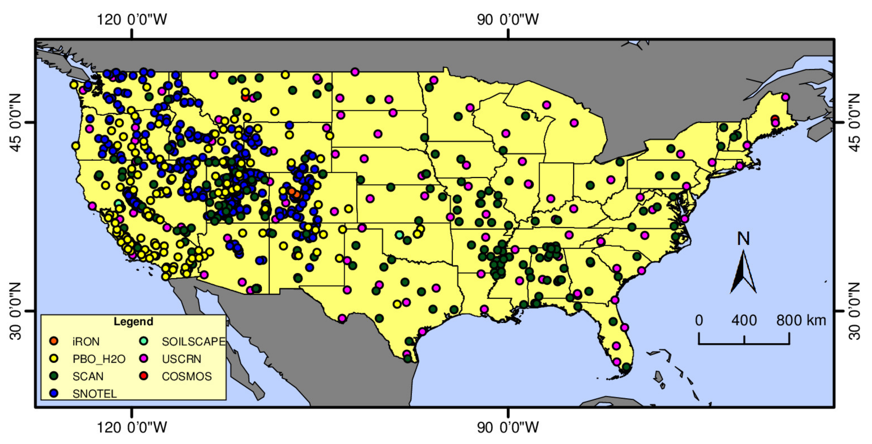
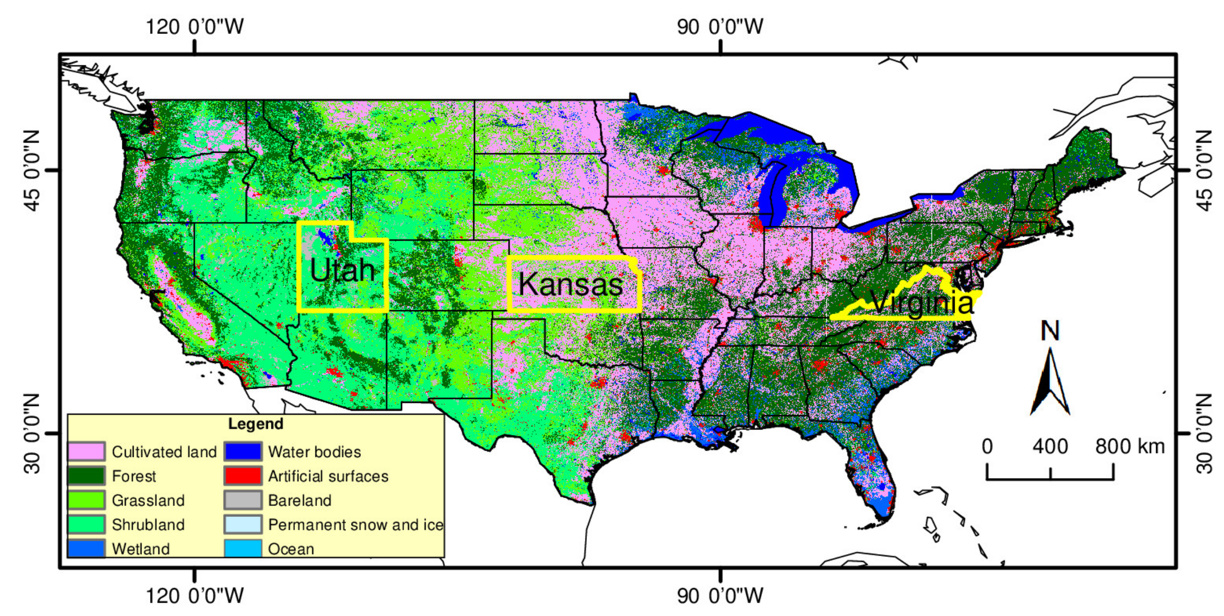
2.1. Study Area
2.2. In-Situ Measurements
2.3. Multi-Source Microwave Remote Sensing Data
2.4. Auxiliary Data
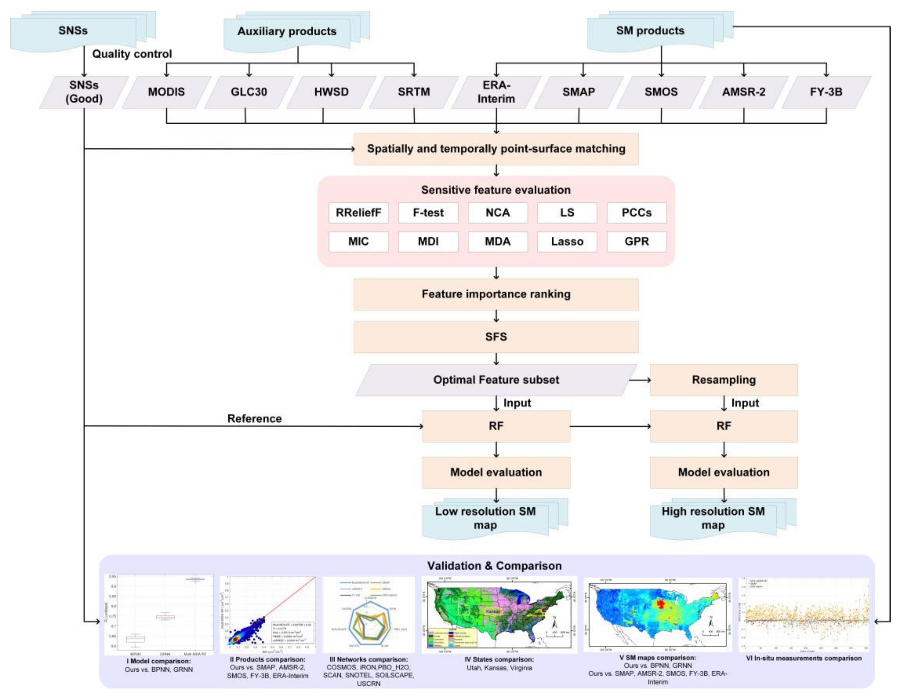
3. Methodology
3.1. Multi-Feature Generation
3.2. Sensitive Feature Evaluation Methods
3.2.1. The Filter Methods
- RReliefF: RReliefF is inspired from Relief [66], which is very powerful in estimating the quality of features [67,68]. RReliefF penalizes the input features that give different values to neighbors with the same response values, and rewards the input features that give different values to neighbors with different response values. We used the 29 features as the input data and the in-situ measurements as the response values. The algorithm selects a random observation and finds the k-nearest observations to it. Then, the weight of SM features can be calculated as follows:where is the weight of having different values for the response y, is the weight of having different values for the feature r, is the weight of having different response values and different values for the feature r, m is the number of iterations. The importance ranking of each feature can be obtained according to this weight.
- F-test: F-test is a statistical test by calculating the f-score of each feature [69]. We examined the importance of each feature individually using F-test, which calculates the values of f-score as follows, and the features were ranked based on f-scores.where p is the p values between features and in-situ measurements.
- NCA: a novel nearest neighbor-based feature selection method was proposed by [70]. This feature selection method performs feature selection with regularization to learn feature weights for minimization of an objective function that measures the average leave-one-out regression loss over the training data. The objective function of minimization is as follows:where n is the number of observations, li is the distance between the in-situ measurements and y, wr the feature weight, λ is the regularization parameter, p is the average accuracy.
- S: Laplacian score is a feature selection algorithm introduced by [71]. The locality preserving power for each feature was reflected by calculating the Laplacian score. Then, we can rank features using the Laplacian scores computed as follows:where ri is the i-th feature, Dg is the degree matrix, and L is the Laplacian matrix.
- PCCs: Pearson correlation coefficient is a simple method that can help to understand the relationship between features and response variables. This method measures the linear correlation between variables. The value range of the result is (−1, 1), where “−1” represents the complete negative correlation, “+1” represents the complete positive correlation, and “0” represents no linear correlation. The feature with the larger absolute value of the correlation is considered more important.
- MIC: MIC is a powerful measure for relevance [72]. It is used to measure the degree of correlation between two variables r and y, and is often used in feature selection of machine learning. MIC can eliminate the feature with less information, so as to make the variable used in model more representative. MIC between the feature r and the response values y can be computed as follows:where I (r; y) is the mutual information between r and y, a, b,is the number of grids in r and y directions, and B is a variable, approximately set to the 0.6th power of the amount of data.
3.2.2. The Embedded Methods
- MDI: RF based feature selection methods can be divided into MDI and MDA [73]. MDI computes feature importance for tree by summing changes in the mean squared error (MSE) due to splits on every feature and dividing the sum by the number of branch nodes. The importance of each feature segmentation is as follows:where Ri is the MSE of each node, Nbranch is the total number of nodes.
- MDA: MDA quantifies variable importance by measuring the change in prediction accuracy when the values of the variable are randomly permuted [74]. The importance of the feature r is then calculated using the following equation:where is the average differences of the features, is the standard deviation of the features.
- Lasso: this method trains a linear regression model with Lasso regularization. For a given value of λ, a nonnegative parameter, Lasso solves the problem:where N is the number of observations, yi is the response at observation i, ri is the i-th feature, a vector of length p at observation i, λ is a nonnegative regularization parameter corresponding to one value of Lambda, and the parameters and are a scalar and a vector of length p, respectively.
- GPR: This method is a feature selection method of GPR model [75]. It trains a GPR model and finds the predictor weights by taking the exponential of the negative learned length scales. Then, we can normalize the weights and obtain the importance ranking.
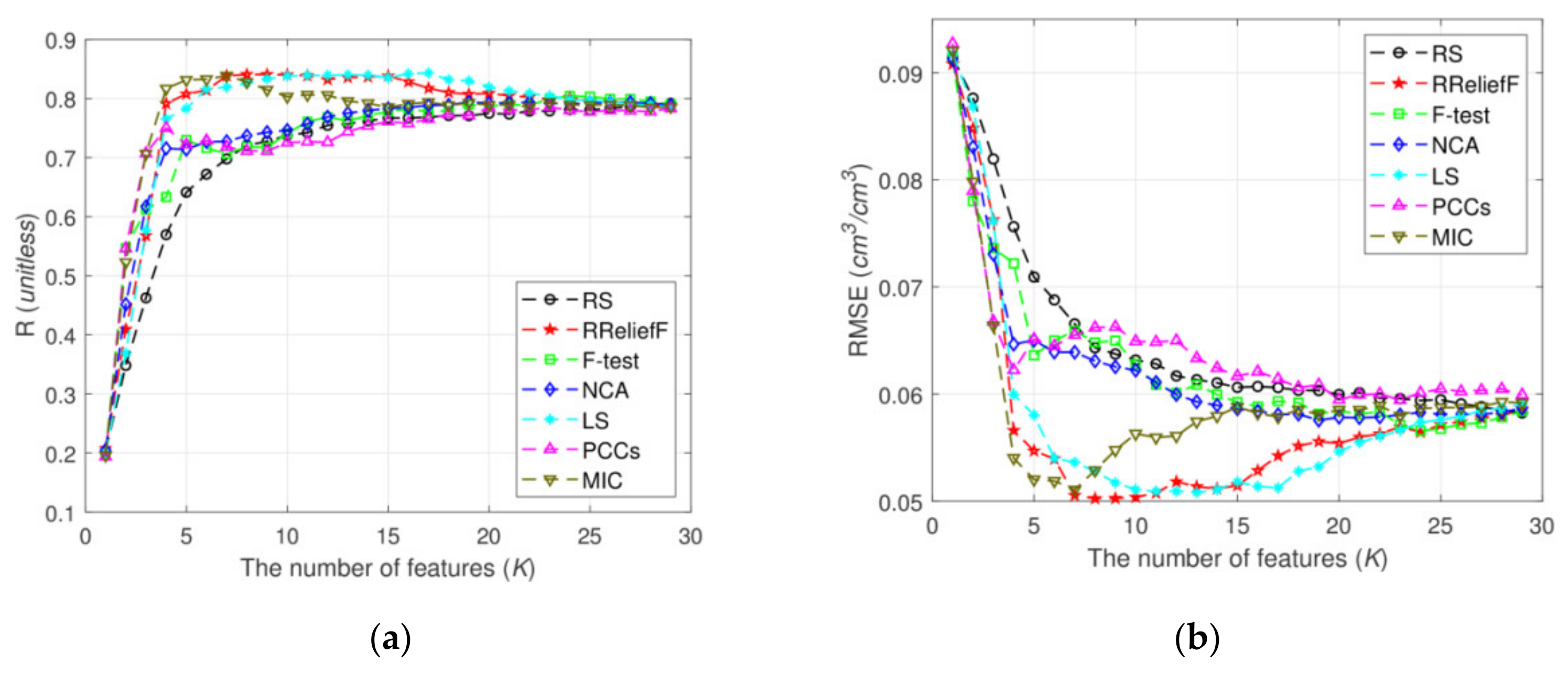
3.2.3. Sequential Forward Selection (SFS)
3.3. The Random Forest (RF) Method
3.4. Evaluation Method
4. Results
4.1. Experimental Settings
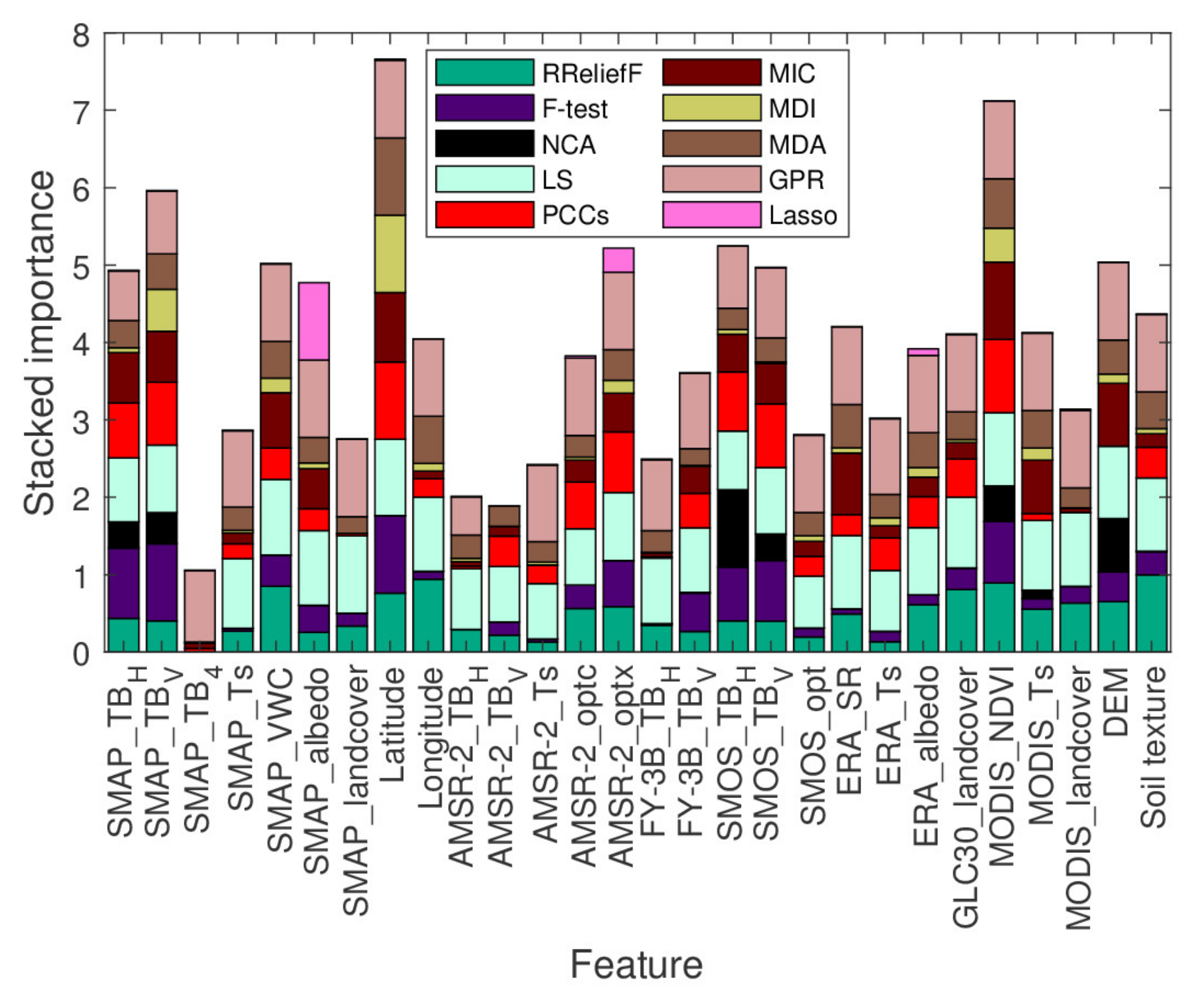
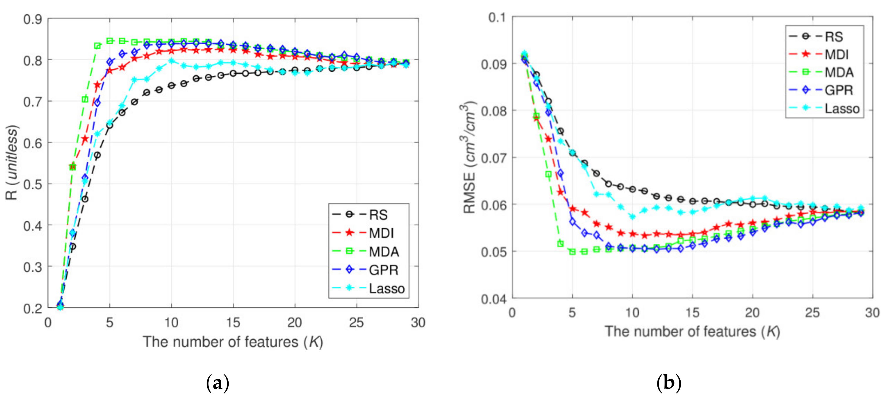
4.2. Selection of Sensitive Features
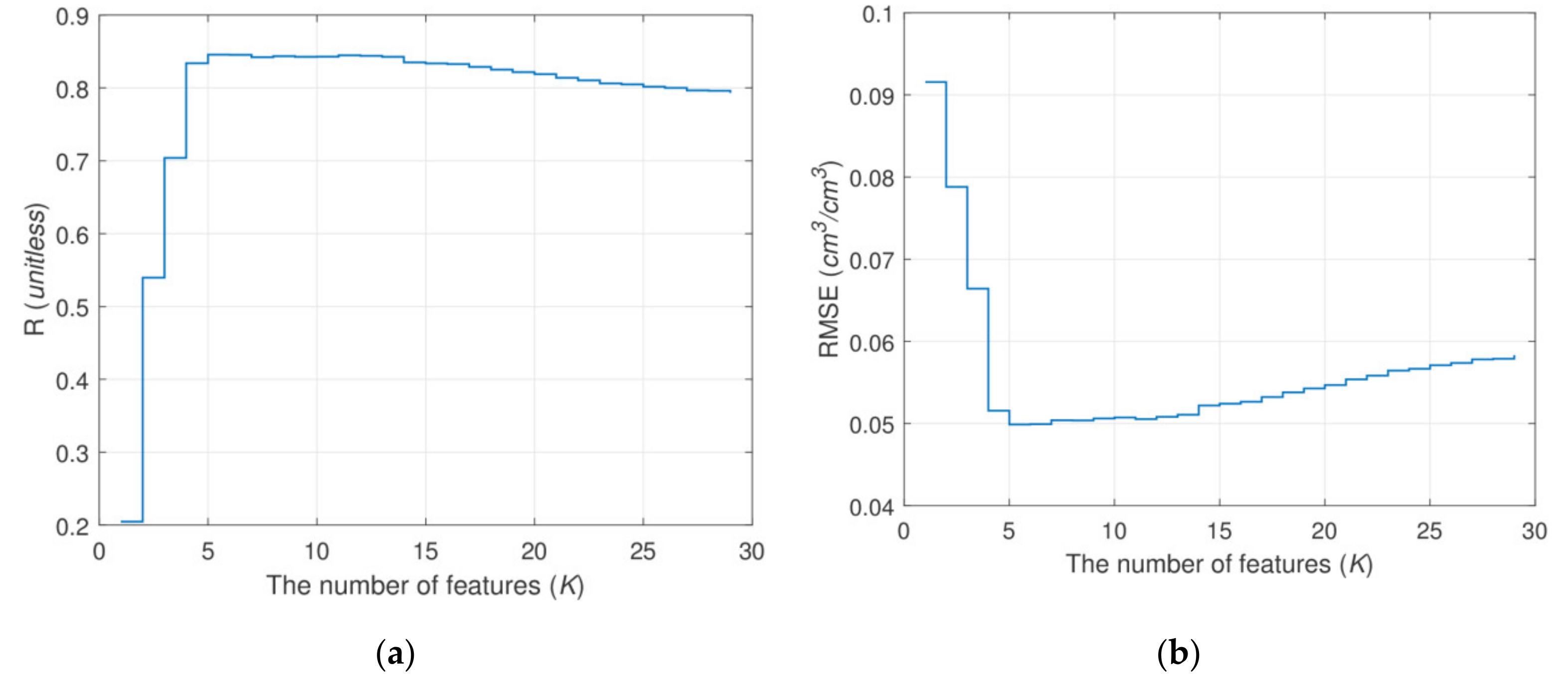
4.3. Parameters Selection for Multi-MDA-RF
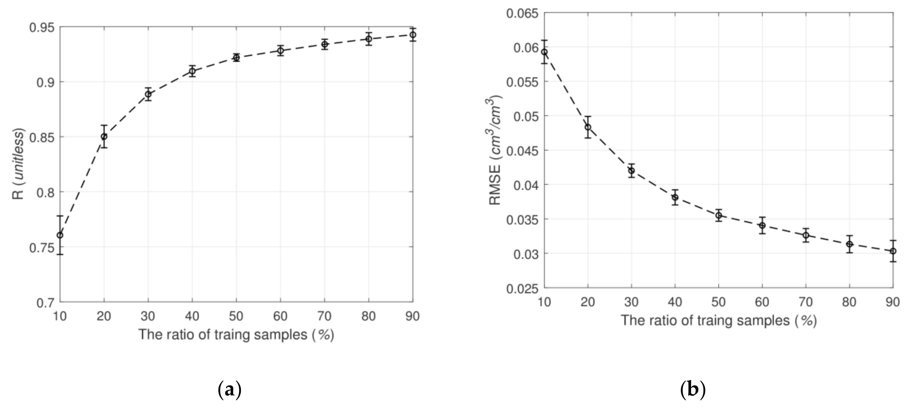
4.4. Generalization Performance Analysis
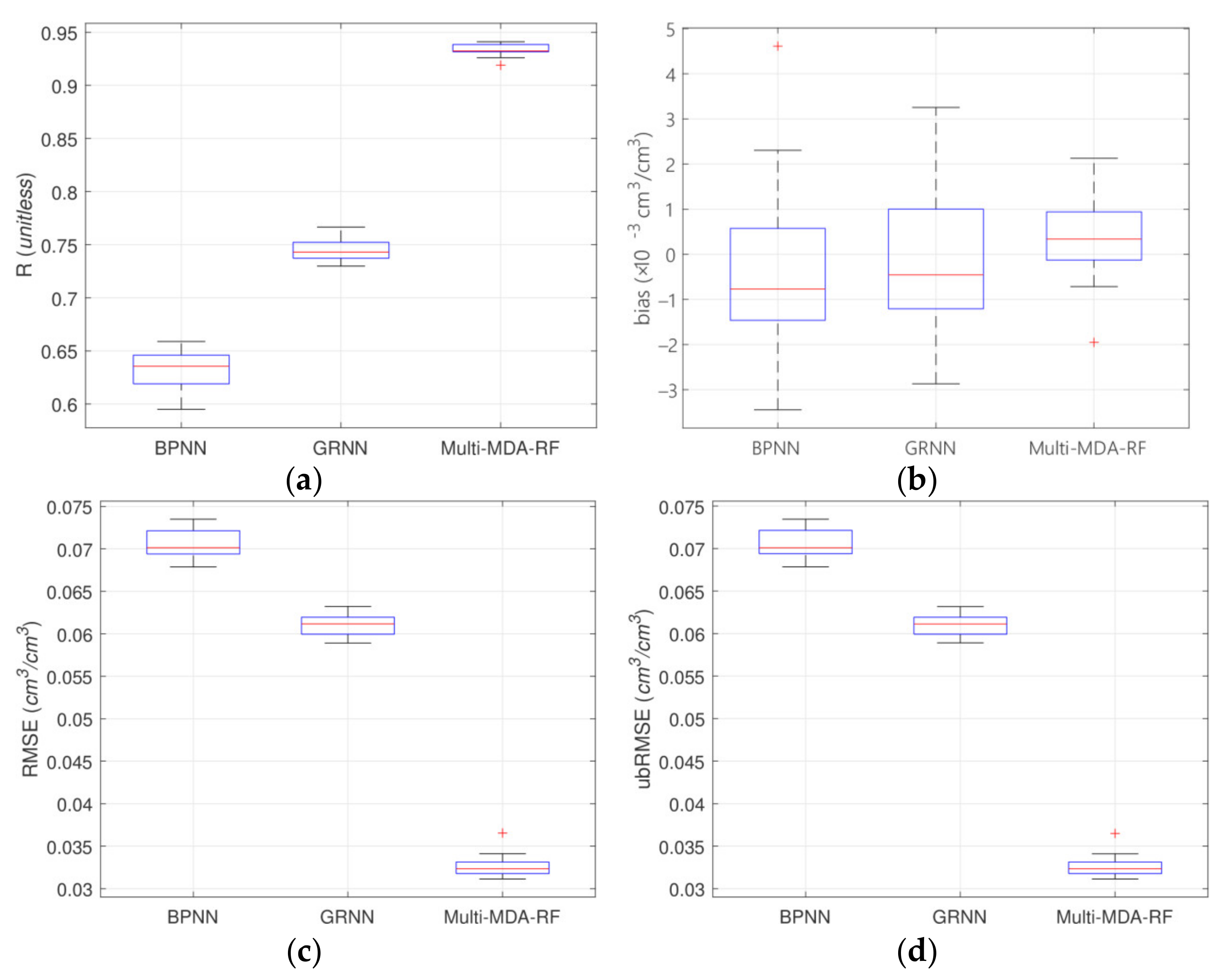
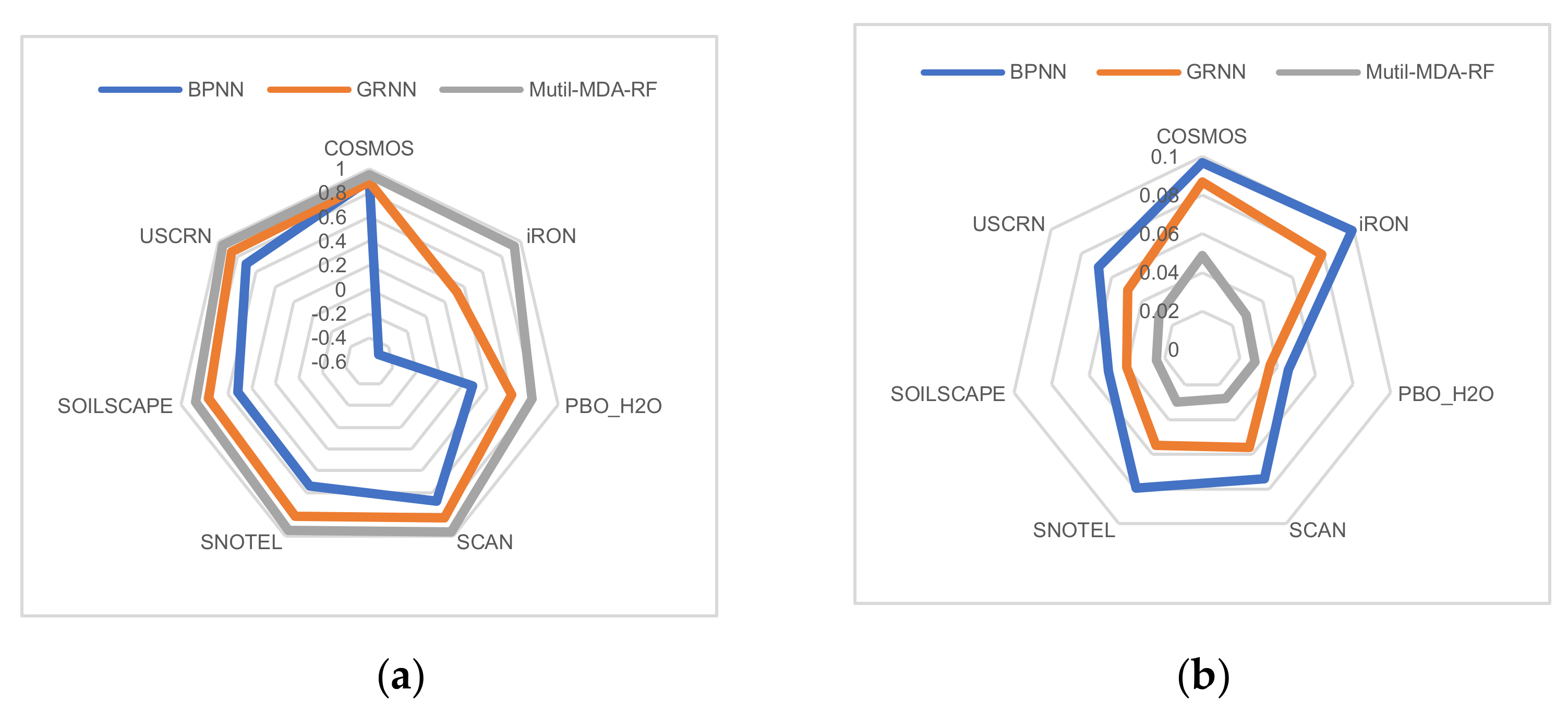
4.5. Evaluation of Different Retrieval Models
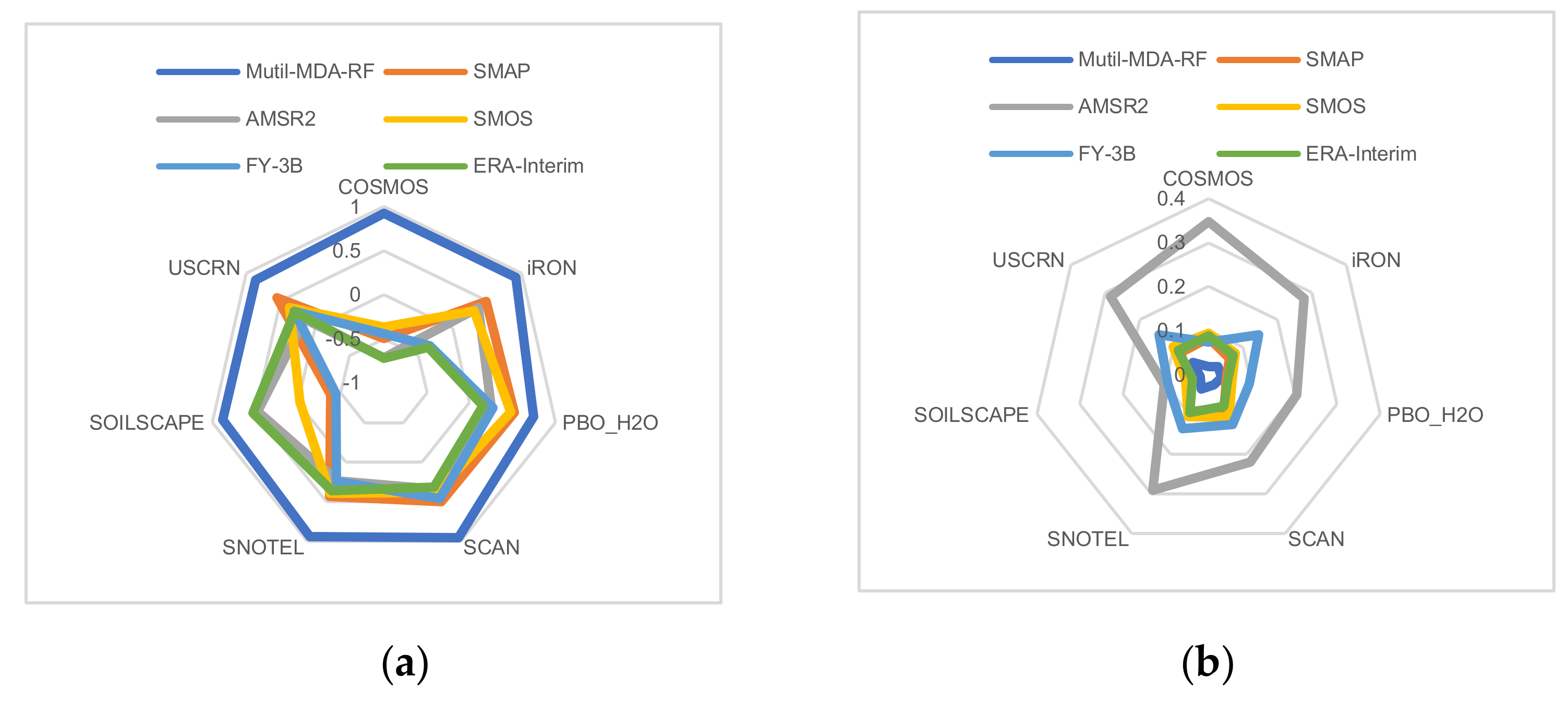
4.6. Evaluation of Different SM Products
4.7. Evaluation of Different SM Networks
4.8. Evaluation of Different U.S. States
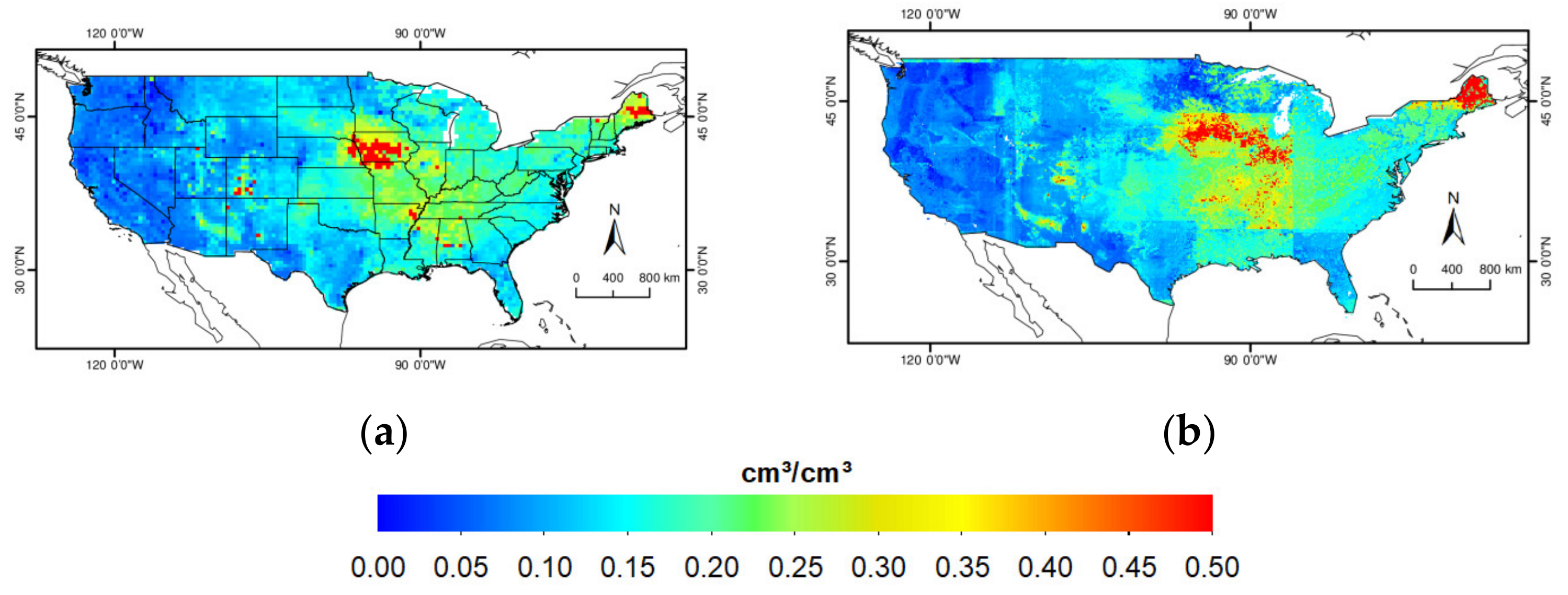
4.9. Producing High Resolution SM Map
5. Discussion
6. Conclusions
Author Contributions
Funding
Institutional Review Board Statement
Informed Consent Statement
Data Availability Statement
Acknowledgments
Conflicts of Interest
References
- Peng, J.; Loew, A.; Merlin, O.; Verhoest, N.E.C. A review of spatial downscaling of satellite remotely sensed soil moisture. Rev. Geophys. 2017, 55, 341–366. [Google Scholar] [CrossRef]
- Kovačević, J.; Cvijetinović, Ž.; Stančić, N.; Brodić, N.; Mihajlović, D. New Downscaling Approach Using ESA CCI SM Products for Obtaining High Resolution Surface Soil Moisture. Remote Sens. 2020, 12, 1119. [Google Scholar] [CrossRef] [Green Version]
- Karthikeyan, L.; Pan, M.; Wanders, N.; Kumar, D.N.; Wood, E.F. Four decades of microwave satellite soil moisture observations: Part 1. A review of retrieval algorithms. Adv. Water Resour. 2017, 109, 106–120. [Google Scholar] [CrossRef]
- Alemohammad, S.H.; Kolassa, J.; Prigent, C.; Aires, F.; Gentine, P. Global downscaling of remotely sensed soil moisture using neural networks. Hydrol. Earth Syst. Sci. 2018, 22, 5341–5356. [Google Scholar] [CrossRef] [Green Version]
- Ge, L.; Hang, R.; Liu, Y.; Liu, Q. Comparing the Performance of Neural Network and Deep Convolutional Neural Network in Estimating Soil Moisture from Satellite Observations. Remote Sens. 2018, 10, 1327. [Google Scholar] [CrossRef] [Green Version]
- Mohanty, B.P.; Cosh, M.H.; Lakshmi, V.; Montzka, C. Soil Moisture Remote Sensing: State-of-the-Science. Vadose Zone J. 2017, 16, 1–9. [Google Scholar] [CrossRef] [Green Version]
- Zeng, J.; Chen, K.-S.; Bi, H.; Chen, Q. A preliminary evaluation of the SMAP radiometer soil moisture product over United States and Europe using ground-based measurements. IEEE Trans. Geosci. Remote Sens. 2016, 54, 4929–4940. [Google Scholar] [CrossRef]
- Kim, S.; Liu, Y.Y.; Johnson, F.M.; Parinussa, R.M.; Sharma, A. A global comparison of alternate AMSR2 soil moisture products: Why do they differ? Remote Sens. Environ. 2015, 161, 43–62. [Google Scholar] [CrossRef]
- Cui, Y.; Long, D.; Hong, Y.; Zeng, C.; Zhou, J.; Han, Z.; Liu, R.; Wan, W. Validation and reconstruction of FY-3B/MWRI soil moisture using an artificial neural network based on reconstructed MODIS optical products over the Tibetan Plateau. J. Hydrol. 2016, 543, 242–254. [Google Scholar] [CrossRef]
- Feng, X.; Li, J.; Cheng, W.; Fu, B.; Wang, Y.; Lü, Y.; Shao, M. Evaluation of AMSR-E retrieval by detecting soil moisture decrease following massive dryland re-vegetation in the Loess Plateau, China. Remote. Sens. Environ. 2017, 196, 253–264. [Google Scholar] [CrossRef]
- Zhuo, L.; Han, D. Multi-source hydrological soil moisture state estimation using data fusion optimisation. Hydrol. Earth Syst. Sci. 2017, 21, 3267–3285. [Google Scholar] [CrossRef] [Green Version]
- Lee, C.S.; Sohn, E.; Park, J.D.; Jang, J.-D. Estimation of soil moisture using deep learning based on satellite data: A case study of South Korea. GIScience Remote. Sens. 2019, 56, 43–67. [Google Scholar] [CrossRef]
- Toride, K.; Sawada, Y.; Aida, K.; Koike, T. Toward high-resolution soil moisture monitoring by combining active-passive microwave and optical vegetation remote sensing products with land surface model. Sensors 2019, 19, 3924. [Google Scholar] [CrossRef] [PubMed] [Green Version]
- Wang, Q.; van der Velde, R.; Ferrazzoli, P.; Chen, X.; Bai, X.; Su, Z. Mapping soil moisture across the Tibetan Plateau plains using Aquarius active and passive L-band microwave observations. Int. J. Appl. Earth Obs. Geoinf. 2019, 77, 108–118. [Google Scholar] [CrossRef]
- Sathyanadh, A.; Karipot, A.; Ranalkar, M.; Prabhakaran, T. Evaluation of soil moisture data products over Indian region and analysis of spatio-temporal characteristics with respect to monsoon rainfall. J. Hydrol. 2016, 542, 47–62. [Google Scholar] [CrossRef]
- Chen, F.; Crow, W.T.; Bindlish, R.; Colliander, A.; Burgin, M.S.; Asanuma, J.; Aida, K. Global-scale evaluation of SMAP, SMOS and ASCAT soil moisture products using triple collocation. Remote Sens. Environ. 2018, 214, 1–13. [Google Scholar] [CrossRef] [PubMed]
- Jing, W.; Song, J.; Zhao, X. Validation of ECMWF Multi-Layer Reanalysis Soil Moisture Based on the OzNet Hydrology Network. Water 2018, 10, 1123. [Google Scholar] [CrossRef] [Green Version]
- Kolassa, J.; Gentine, P.; Prigent, C.; Aires, F.; Alemohammad, S. Soil moisture retrieval from AMSR-E and ASCAT microwave observation synergy. Part 2: Product evaluation. Remote Sens. Environ. 2017, 195, 202–217. [Google Scholar] [CrossRef]
- Kim, H.; Parinussa, R.; Konings, A.G.; Wagner, W.; Cosh, M.H.; Lakshmi, V.; Zohaib, M.; Choi, M. Global-scale assessment and combination of SMAP with ASCAT (active) and AMSR2 (passive) soil moisture products. Remote Sens. Environ. 2018, 204, 260–275. [Google Scholar] [CrossRef]
- Bulut, B.; Yilmaz, M.T.; Afshar, M.H.; Şorman, A.Ü.; Yücel, I.; Cosh, M.H.; Şimşek, O. Evaluation of Remotely-Sensed and Model-Based Soil Moisture Products According to Different Soil Type, Vegetation Cover and Climate Regime Using Station-Based Observations over Turkey. Remote Sens. 2019, 11, 1875. [Google Scholar] [CrossRef] [Green Version]
- Duygu, M.B.; Akyürek, Z. Using cosmic-ray neutron probes in validating satellite soil moisture products and land surface models. Water 2019, 11, 1362. [Google Scholar] [CrossRef] [Green Version]
- Qu, Y.; Zhu, Z.; Chai, L.; Liu, S.; Montzka, C.; Liu, J.; Yang, X.; Lu, Z.; Jin, R.; Li, X.; et al. Rebuilding a Microwave Soil Moisture Product Using Random Forest Adopting AMSR-E/AMSR2 Brightness Temperature and SMAP over the Qinghai–Tibet Plateau, China. Remote Sens. 2019, 11, 683. [Google Scholar] [CrossRef] [Green Version]
- Kerr, Y.H.; Al-Yaari, A.; Rodriguez-Fernandez, N.; Parrens, M.; Molero, B.; Leroux, D.; Bircher, S.; Mahmoodi, A.; Mialon, A.; Richaume, P.; et al. Overview of SMOS performance in terms of global soil moisture monitoring after six years in operation. Remote Sens. Environ. 2016, 180, 40–63. [Google Scholar] [CrossRef]
- Agutu, N.O.; Awange, J.L.; Ndehedehe, C.; Mwaniki, M. Consistency of agricultural drought characterization over Upper Greater Horn of Africa (1982–2013): Topographical, gauge density, and model forcing influence. Sci. Total Environ. 2020, 709, 135149. [Google Scholar] [CrossRef]
- Hagan, D.F.T.; Parinussa, R.M.; Wang, G.; Draper, C.S. An evaluation of soil moisture anomalies from global model-based datasets over the people’s republic of China. Water 2020, 12, 117. [Google Scholar] [CrossRef] [Green Version]
- Sahebi, M.R.; Angles, J. An inversion method based on multi-angular approaches for estimating bare soil surface parameters from RADARSAT-1. Hydrol. Earth Syst. Sci. 2010, 14, 2355–2366. [Google Scholar] [CrossRef] [Green Version]
- Baghdadi, N.; Chaaya, J.A.; Zribi, M. Semiempirical Calibration of the Integral Equation Model for SAR Data in C-Band and Cross Polarization Using Radar Images and Field Measurements. IEEE Geosci. Remote Sens. Lett. 2010, 8, 14–18. [Google Scholar] [CrossRef] [Green Version]
- Kseneman, M.; Gleich, D.; Cucej, Ž. Soil moisture estimation using high-resolution spotlight TerraSAR-X data. IEEE Geosci. Remote Sens. Lett. 2011, 8, 686–690. [Google Scholar] [CrossRef]
- Lievens, H.; Verhoest, N.E.C. On the retrieval of soil moisture in wheat fields from L-Band SAR based on water cloud modeling, the IEM, and effective roughness parameters. IEEE Geosci. Remote Sens. Lett. 2011, 8, 740–744. [Google Scholar] [CrossRef]
- Merzouki, A.; McNairn, H.; Pacheco, A. Mapping soil moisture using RADARSAT-2 data and local autocorrelation statistics. IEEE J. Sel. Top. Appl. Earth Obs. Remote Sens. 2011, 4, 128–137. [Google Scholar] [CrossRef]
- Wang, S.G.; Li, X.; Han, X.J.; Jin, R. Estimation of surface soil moisture and roughness from multi-angular ASAR imagery in the Watershed Allied Telemetry Experimental Research (WATER). Hydrol. Earth Syst. Sci. 2011, 15, 1415–1426. [Google Scholar] [CrossRef] [Green Version]
- Shen, X.; Mao, K.; Qin, Q.; Hong, Y.; Zhang, G. Bare surface soil moisture estimation using Double-Angle and dual-polarization L-Band radar data. IEEE Trans. Geosci. Remote Sens. 2013, 51, 3931–3942. [Google Scholar] [CrossRef]
- Chakravorty, A.; Chahar, B.R.; Sharma, O.P.; Dhanya, C.T. A regional scale performance evaluation of SMOS and ESA-CCI soil moisture products over India with simulated soil moisture from MERRA-Land. Remote Sens. Environ. 2016, 186, 514–527. [Google Scholar] [CrossRef]
- Wigneron, J.P.; Jackson, T.J.; O’Neill, P.; De Lannoy, G.; de Rosnay, P.; Walker, J.P.; Ferrazzoli, P.; Mironov, V.; Bircher, S.; Grant, J.P.; et al. Modelling the passive microwave signature from land surfaces: A review of recent results and application to the L-band SMOS & SMAP soil moisture retrieval algorithms. Remote Sens. Environ. 2017, 192, 238–262. [Google Scholar]
- Das, N.; Entekhabi, D.; Dunbar, R.; Chaubell, M.; Colliander, A.; Yueh, S.; Jagdhuber, T.; Chen, F.; Crow, W.; O’Neill, P.; et al. The SMAP and Copernicus Sentinel 1A/B microwave active-passive high resolution surface soil moisture product. Remote Sens. Environ. 2019, 233, 111380. [Google Scholar] [CrossRef]
- Karthikeyan, L.; Pan, M.; Konings, A.G.; Piles, M.; Fernandez-Moran, R.; Kumar, D.N.; Wood, E.F. Simultaneous retrieval of global scale Vegetation Optical Depth, surface roughness, and soil moisture using X-band AMSR-E observations. Remote Sens. Environ. 2019, 234, 111473. [Google Scholar] [CrossRef]
- Azimi, S.; Dariane, A.B.; Modanesi, S.; Bauer-Marschallinger, B.; Bindlish, R.; Wagner, W.; Massari, C. Assimilation of Sentinel 1 and SMAP—Based satellite soil moisture retrievals into SWAT hydrological model: The impact of satellite revisit time and product spatial resolution on flood simulations in small basins. J. Hydrol. 2020, 581, 124367. [Google Scholar] [CrossRef] [PubMed]
- Kolassa, J.; Reichle, R.H.; Liu, Q.; Alemohammad, S.H.; Gentine, P.; Aida, K.; Asanuma, J.; Bircher, S.; Caldwell, T.; Colliander, A.; et al. Estimating surface soil moisture from SMAP observations using a Neural Network technique. Remote Sens. Environ. 2018, 204, 43–59. [Google Scholar] [CrossRef]
- Cui, Y.; Chen, X.; Xiong, W.; He, L.; Lv, F.; Fan, W.; Luo, Z.; Hong, Y. A Soil Moisture Spatial and Temporal Resolution Improving Algorithm Based on Multi-Source Remote Sensing Data and GRNN Model. Remote Sens. 2020, 12, 455. [Google Scholar] [CrossRef] [Green Version]
- Xu, H.; Yuan, Q.; Li, T.; Shen, H.; Zhang, L.; Jiang, H. Quality Improvement of Satellite Soil Moisture Products by Fusing with In-Situ Measurements and GNSS-R Estimates in the Western Continental U.S. Remote Sens. 2018, 10, 1351. [Google Scholar] [CrossRef] [Green Version]
- Eroglu, O.; Kurum, M.; Boyd, D.; Gurbuz, A.C. High Spatio-Temporal Resolution CYGNSS Soil Moisture Estimates Using Artificial Neural Networks. Remote Sens. 2019, 11, 2272. [Google Scholar] [CrossRef] [Green Version]
- Ma, C.; Li, X.; Wei, L.; Wang, W. Multi-scale validation of SMAP soil moisture products over cold and arid regions in northwestern China using distributed ground observation data. Remote Sens. 2017, 9, 327. [Google Scholar] [CrossRef] [Green Version]
- Yuan, Q.; Shen, H.; Li, T.; Li, Z.; Li, S.; Jiang, Y.; Xu, H.; Tan, W.; Yang, Q.; Wang, J.; et al. Deep learning in environmental remote sensing: Achievements and challenges. Remote Sens. Environ. 2020, 241, 111716. [Google Scholar] [CrossRef]
- Yuan, Q.; Xu, H.; Li, T.; Shen, H.; Zhang, L. Estimating surface soil moisture from satellite observations using a generalized regression neural network trained on sparse ground-based measurements in the continental U.S. J. Hydrol. 2020, 580, 125843. [Google Scholar] [CrossRef]
- Senyurek, V.; Lei, F.; Boyd, D.; Kurum, M.; Gurbuz, A.C.; Moorhead, R. Machine Learning-Based CYGNSS Soil Moisture Estimates over ISMN sites in CONUS. Remote Sens. 2020, 12, 1168. [Google Scholar] [CrossRef] [Green Version]
- Fang, K.; Shen, C.; Kifer, D.; Yang, X. Prolongation of SMAP to Spatiotemporally Seamless Coverage of Continental U.S. Using a Deep Learning Neural Network. Geophys. Res. Lett. 2017, 44, 11030–11039. [Google Scholar] [CrossRef] [Green Version]
- Zreda, M.; Desilets, D.; Ferre, T.P.A.; Scott, R.L. Measuring soil moisture content non-invasively at intermediate spatial scale using cosmic-ray neutrons. Geophys. Res. Lett. 2008, 35. [Google Scholar] [CrossRef] [Green Version]
- Zreda, M.; Shuttleworth, W.J.; Zeng, X.; Zweck, C.; Desilets, D.; Franz, T.E.; Rosolem, R. COSMOS: The COsmic-ray Soil Moisture Observing System. Hydrol. Earth Syst. Sci. 2012, 16, 4079–4099. [Google Scholar] [CrossRef] [Green Version]
- Montzka, C.; Bogena, H.R.; Zreda, M.; Monerris, A.; Morrison, R.; Muddu, S.; Vereecken, H. Validation of Spaceborne and Modelled Surface Soil Moisture Products with Cosmic-Ray Neutron Probes. Remote Sens. 2017, 9, 103. [Google Scholar] [CrossRef] [Green Version]
- Osenga, E.C.; Arnott, J.C.; Endsley, K.A.; Katzenberger, J.W. Bioclimatic and Soil Moisture Monitoring Across Elevation in a Mountain Watershed: Opportunities for Research and Resource Management. Water Resour. Res. 2019, 55, 2493–2503. [Google Scholar] [CrossRef]
- Larson, K.M.; Small, E.; Gutmann, E.; Bilich, A.L.; Braun, J.J.; Zavorotny, V.U. Use of GPS receivers as a soil moisture network for water cycle studies. Geophys. Res. Lett. 2008, 35. [Google Scholar] [CrossRef] [Green Version]
- Schaefer, G.L.; Cosh, M.H.; Jackson, T.J. The USDA Natural Resources Conservation Service Soil Climate Analysis Network (SCAN). J. Atmos. Ocean. Technol. 2007, 24, 2073–2077. [Google Scholar] [CrossRef]
- Lu, Y.; Wei, C. Evaluation of microwave soil moisture data for monitoring live fuel moisture content (LFMC) over the coterminous United States. Sci. Total. Environ. 2021, 771, 145410. [Google Scholar] [CrossRef]
- Leavesley, G.; David, O.; Garen, D.; Lea, J.; Marron, J.; Pagano, T.; Perkins, T.; Strobel, M. A Modeling Framework for Improved Agricultural Water Supply Forecasting. AGU Fall Meeting, San Francisco, CA, USA, 15–19 December 2008; Volume 2008, p. C21A-0497. [Google Scholar]
- Moghaddam, M.; Entekhabi, D.; Goykhman, Y.; Li, K.; Liu, M.Y.; Mahajan, A.; Nayyar, A.; Shuman, D.; Teneketzis, D. A Wireless Soil Moisture Smart Sensor Web Using Physics-Based Optimal Control: Concept and Initial Demonstrations. IEEE J. Sel. Top. Appl. Earth Obs. Remote Sens. 2010, 3, 522–535. [Google Scholar] [CrossRef]
- Bell, J.E.; Palecki, M.A.; Baker, C.B.; Collins, W.G.; Lawrimore, J.H.; Leeper, R.; Hall, M.E.; Kochendorfer, J.; Meyers, T.P.; Wilson, T.; et al. U.S. Climate Reference Network Soil Moisture and Temperature Observations. J. Hydrometeorol. 2013, 14, 977–988. [Google Scholar] [CrossRef]
- Dorigo, W.; Wagner, W.; Hohensinn, R.; Hahn, S.; Paulik, C.; Xaver, A.; Gruber, A.; Drusch, M.; Mecklenburg, S.; Van Oevelen, P.; et al. The International Soil Moisture Network: A data hosting facility for global in situ soil moisture measurements. Hydrol. Earth Syst. Sci. 2011, 15, 1675–1698. [Google Scholar] [CrossRef] [Green Version]
- Dorigo, W.A.; Xaver, A.; Vreugdenhil, M.; Gruber, A.; Hegyiová, A.; Sanchis-Dufau, A.D.; Zamojski, D.; Cordes, C.; Wagner, W.; Drusch, M. Global Automated Quality Control of In Situ Soil Moisture Data from the International Soil Moisture Network. Vadose Zone J. 2013, 12. [Google Scholar] [CrossRef]
- Chen, Q.; Zeng, J.; Cui, C.; Li, Z.; Chen, K.-S.; Bai, X.; Xu, J. Soil Moisture Retrieval From SMAP: A Validation and Error Analysis Study Using Ground-Based Observations Over the Little Washita Watershed. IEEE Trans. Geosci. Remote Sens. 2017, 56, 1394–1408. [Google Scholar] [CrossRef]
- Singh, G.; Das, N.N.; Panda, R.K.; Colliander, A.; Jackson, T.J.; Mohanty, B.P.; Entekhabi, D.; Yueh, S.H. Validation of SMAP Soil Moisture Products Using Ground-Based Observations for the Paddy Dominated Tropical Region of India. IEEE Trans. Geosci. Remote Sens. 2019, 57, 8479–8491. [Google Scholar] [CrossRef]
- Bindlish, R.; Caldwell, T.; Collins, C.H.; McNairn, H.; Martinez-Fernandez, J.; Prueger, J.; Rowlandson, T.; Seyfried, M.; Starks, P.; Thibeault, M.; et al. GCOM-W AMSR2 soil moisture product validation using core validation sites. IEEE J. Sel. Top. Appl. Earth Obs. Remote Sens. 2018, 11, 209–219. [Google Scholar] [CrossRef] [Green Version]
- Peng, J.; Misra, S.; Piepmeier, J.R.; Dinnat, E.P.; Hudson, D.; Le Vine, D.M.; De Amici, G.; Mohammed, P.N.; Bindlish, R.; Yueh, S.H.; et al. Soil moisture active/passive L-Band microwave radiometer postlaunch calibration. IEEE Trans. Geosci. Remote Sens. 2017, 55, 5339–5354. [Google Scholar] [CrossRef]
- Liu, J.; Chai, L.; Lu, Z.; Liu, S.; Qu, Y.; Geng, D.; Song, Y.; Guan, Y.; Guo, Z.; Wang, J.; et al. Evaluation of SMAP, SMOS-IC, FY3B, JAXA, and LPRM soil moisture products over the Qinghai-Tibet Plateau and its surrounding areas. Remote Sens. 2019, 11, 792. [Google Scholar] [CrossRef] [Green Version]
- Zeng, J.; Li, Z.; Chen, Q.; Bi, H.; Qiu, J.; Zou, P. Evaluation of remotely sensed and reanalysis soil moisture products over the Tibetan Plateau using in-situ observations. Remote Sens. Environ. 2015, 163, 91–110. [Google Scholar] [CrossRef]
- Guyon, I.; Elisseeff, A. An Introduction of Variable and Feature Selection. J. Mach. Learn. Res. 2003, 3, 1157–1182. [Google Scholar]
- Kira, K.; Rendell, L. The Feature Selection Problem: Traditional Methods and a New Algorithm. In Proceedings of the Tenth National Conference on Artificial Intelligence (AAAI’92), San Jose, CA, USA, 12–16 July 1992. [Google Scholar]
- Robnik-Sikonja, M.; Kononenko, I. An adaptation of Relief for attribute estimation in regression. In Proceedings of the Fourteenth International Conference on Machine Learning (ICML’97), Nashville, TN, USA, 8–12 July 2000. [Google Scholar]
- Robnik-Šikonja, M.; Kononenko, I. Theoretical and Empirical Analysis of ReliefF and RReliefF. Mach. Learn. 2003, 53, 23–69. [Google Scholar] [CrossRef] [Green Version]
- Dhanya, R.; Paul, I.R.; Akula, S.S.; Sivakumar, M.; Nair, J.J. F-test feature selection in Stacking ensemble model for breast cancer prediction. Procedia Comput. Sci. 2020, 171, 1561–1570. [Google Scholar] [CrossRef]
- Yang, W.; Wang, K.; Zuo, W. Neighborhood Component Feature Selection for High-Dimensional Data. JCP 2012, 7, 161–168. [Google Scholar] [CrossRef]
- He, X.; Cai, D.; Niyogi, P. Laplacian score for feature selection. In Proceedings of the 18th International Conference on Neural Information Processing Systems (NIPS’05), Vancouver, BC, Canada, 5–8 December 2005. [Google Scholar]
- Petković, M.; Kocev, D.; Džeroski, S. Feature ranking for multi-target regression. Mach. Learn. 2019, 109, 1179–1204. [Google Scholar] [CrossRef]
- Gwetu, M.V.; Tapamo, J.-R.; Viriri, S. Exploring the impact of purity gap gain on the efficiency and effectiveness of random forest feature selection. In Proceedings of the International Conference on Computational Collective Intelligence (ICCCI’19), Hendaye, France, 4–6 September 2019; pp. 340–352. [Google Scholar]
- Behnamian, A.; Millard, K.; Banks, S.N.; White, L.; Richardson, M.; Pasher, J. A Systematic Approach for Variable Selection With Random Forests: Achieving Stable Variable Importance Values. IEEE Geosci. Remote Sens. Lett. 2017, 14, 1988–1992. [Google Scholar] [CrossRef] [Green Version]
- Rasmussen, C.; Williams, C. Gaussian Process for Machine Learning; The MIT Press: Cambridge, MA, USA, 2006. [Google Scholar]
- Marcano-Cedeño, A.; Quintanilla, J.; Cortina-Januchs, G.; Andina, D. Feature selection using sequential forward selection and classification applying artificial metaplasticity neural network. In Proceedings of the IECON 2010-36th Annual Conference on IEEE Industrial Electronics Society, Glendale, AZ, USA, 7–10 November 2010. [Google Scholar]
- Breiman, L. Random Forests. Mach. Learn. 2001, 45, 5–32. [Google Scholar] [CrossRef] [Green Version]
- Entekhabi, D.; Reichle, R.H.; Koster, R.D.; Crow, W.T. Performance Metrics for Soil Moisture Retrievals and Application Requirements. J. Hydrometeorol. 2010, 11, 832–840. [Google Scholar] [CrossRef]
- Ma, H.; Zeng, J.; Chen, N.; Zhang, X.; Cosh, M.H.; Wang, W. Satellite surface soil moisture from SMAP, SMOS, AMSR2 and ESA CCI: A comprehensive assessment using global ground-based observations. Remote Sens. Environ. 2019, 231. [Google Scholar] [CrossRef]
- Ge, X.; Wang, J.; Ding, J.; Cao, X.; Zhang, Z.; Liu, J.; Li, X. Combining UAV-based hyperspectral imagery and machine learning algorithms for soil moisture content monitoring. PeerJ 2019, 7, e6926. [Google Scholar] [CrossRef] [PubMed]
- Yang, X.; Zhang, C.; Cui, Z.; Yu, F.; Wang, J.; Han, Y. Filling method for soil moisture based on BP neural network. J. Appl. Remote Sens. 2018, 12, 042806. [Google Scholar]
- Chatterjee, S.; Huang, J.; Hartemink, A.E. Establishing an Empirical Model for Surface Soil Moisture Retrieval at the U.S. Climate Reference Network Using Sentinel-1 Backscatter and Ancillary Data. Remote Sens. 2020, 12, 1242. [Google Scholar] [CrossRef] [Green Version]


| Network | Sites (Total) | Sites (Used) | Available Time | Depth (cm) | Temporal Resolution | Sensor |
|---|---|---|---|---|---|---|
| COSMOS | 109 | 6 | 28 April 2008–29 March 2020 | 0–10 | Hourly | Cosmic-ray Probe |
| iRON | 9 | 9 | 21 August 2012–1 January 2020 | 5 | Hourly | EC5 II, 10HS, EC5 I, HMP155, EC5 |
| PBO_H2O | 159 | 140 | 27 September 2004–16 December 2017 | 0–5 | Daily | GPS |
| SCAN | 239 | 188 | 1 January 1996–Now | 5 | Hourly | n.s., 5.0 Volt, 2.5 Volt, linear |
| SNOTEL | 441 | 130 | 1 October 1980–Now | 5 | Hourly | n.s., 5.0 Volt, 2.5 Volt |
| SOILSCAPE | 171 | 114 | 3 August 2011–29 March 2017 | 5 | Hourly | EC5 |
| USCRN | 115 | 113 | 15 November 2000–Now | 5 | Hourly | Stevens HydraProbe II Sdi-12 |
| Microwave Remote Sensing Product | Band | Spatial Resolution (km) | Temporal Resolution (days) | Available Time | Orbit |
|---|---|---|---|---|---|
| SMAP | L | 36 | ~3 | April 2015–Now | 6:00 p.m. (A) 6:00 a.m. (D) |
| SMOS | L | 25 | ~3 | January 2010–Now | 6:00 a.m. (A) 6:00 p.m. (D) |
| AMSR2 | C/X | 25 | ~2 | July 2012–Now | 1:30 p.m. (A) 1:30 a.m. (D) |
| FY-3B | X/Ku/K/Ka/E | 25 | ~2 | July 2011–June 2020 | 1:40 p.m. (A) 1:40 a.m. (D) |
| Data | Index | Feature | Spatial Resolution | Description |
|---|---|---|---|---|
| SMAP | 1 | SMAP_TBH | 36 km | Brightness temperatures (H) |
| 2 | SMAP_TBV | Brightness temperatures (V) | ||
| 3 | SMAP_TB4 | 4th Stokes’ parameters | ||
| 4 | SMAP_Ts | Daily surface temperature | ||
| 5 | SMAP_VWC | Daily vegetation water content | ||
| 6 | SMAP_albedo | Daily single-scattering albedo | ||
| 7 | SMAP_landcover | Daily landcover classification | ||
| 8 | Latitude | Center latitude | ||
| 9 | Longitude | Center longitude | ||
| AMSR2 | 10 | AMSR2_TBH | 25 km | C-band brightness temperatures (H) |
| 11 | AMSR2_TBV | C-band brightness temperatures (V) | ||
| 12 | AMSR2_Ts | C-band daily surface temperature | ||
| 13 | AMSR2_optc | C-band optical depth | ||
| 14 | AMSR2_optx | X-band optical depth | ||
| FY-3B | 15 | FY-3B_TBH | 25 km | X-band brightness temperatures (H) |
| 16 | FY-3B_TBV | X-band brightness temperatures (V) | ||
| SMOS | 17 | SMOS_TBH | 25 km | Brightness temperatures (H) |
| 18 | SMOS_TBV | Brightness temperatures (V) | ||
| 19 | SMOS_opt | optical depth | ||
| ERA-Interim | 20 | ERA_SR | 0.125° | Daily surface roughness |
| 21 | ERA_Ts | Daily surface temperature | ||
| 22 | ERA_albedo | Daily albedo | ||
| GlobeLand30 | 23 | GLC30_landcover | 30 m | Landcover classification (2010) |
| MODIS | 24 | MODIS_NDVI | 0.05° | Monthly Normalized Difference Vegetation Index |
| 25 | MODIS_Ts | Monthly night surface temperature | ||
| 26 | MODIS_landcover | Landcover classification (2015) | ||
| SRTM | 27 | DEM | 90 m | Elevation |
| HWSD | 28 | Soil texture | 1 km | Soil texture (FAO74) |
| DOY | 29 | DOY | \ | Day of year |
| Feature | The Importance Ranking | |||||||||
|---|---|---|---|---|---|---|---|---|---|---|
| Filter | Embedded | |||||||||
| RReliefF | F-Test | NCA | LS | PCCs | MIC | MDI | MDA | GPR | Lasso | |
| SMAP_TBH | 14 | 3 | 6 | 20 | 7 | 8 | 15 | 13 | 26 | 10 |
| SMAP_TBV | 16 | 2 | 4 | 15 | 4 | 7 | 2 | 8 | 24 | 26 |
| SMAP_TB4 | 28 | 28 | 16 | 28 | 23 | 23 | 22 | 28 | 21 | 11 |
| SMAP_Ts | 21 | 24 | 18 | 13 | 21 | 20 | 20 | 18 | 18 | 12 |
| SMAP_VWC | 4 | 9 | 13 | 3 | 12 | 5 | 4 | 6 | 13 | 13 |
| SMAP_albedo | 23 | 11 | 25 | 4 | 16 | 10 | 11 | 14 | 1 | 1 |
| SMAP_landcover | 19 | 17 | 9 | 1 | 25 | 28 | 27 | 27 | 2 | 14 |
| Latitude | 6 | 1 | 20 | 2 | 1 | 2 | 1 | 1 | 3 | 6 |
| Longitude | 2 | 22 | 15 | 5 | 19 | 22 | 10 | 3 | 4 | 27 |
| AMSR2_TBH | 20 | 27 | 28 | 22 | 24 | 24 | 17 | 17 | 27 | 15 |
| AMSR2_TBV | 24 | 16 | 27 | 26 | 15 | 21 | 28 | 24 | 28 | 23 |
| AMSR2_Ts | 27 | 25 | 14 | 25 | 20 | 27 | 21 | 23 | 17 | 16 |
| AMSR2_optc | 11 | 12 | 21 | 24 | 8 | 14 | 19 | 21 | 15 | 4 |
| AMSR2_optx | 10 | 7 | 22 | 14 | 5 | 11 | 5 | 11 | 14 | 2 |
| FY-3B_TBH | 18 | 26 | 17 | 18 | 26 | 26 | 26 | 20 | 22 | 7 |
| FY-3B_TBV | 22 | 8 | 8 | 19 | 10 | 13 | 24 | 26 | 20 | 17 |
| SMOS_TBH | 15 | 6 | 1 | 23 | 6 | 12 | 16 | 22 | 25 | 28 |
| SMOS_TBV | 17 | 5 | 5 | 17 | 3 | 9 | 23 | 15 | 23 | 18 |
| SMOS_opt | 25 | 21 | 23 | 27 | 18 | 17 | 12 | 16 | 16 | 19 |
| ERA_SR | 13 | 23 | 10 | 9 | 17 | 4 | 14 | 4 | 5 | 25 |
| ERA_Ts | 26 | 19 | 26 | 21 | 11 | 19 | 9 | 19 | 19 | 20 |
| ERA_albedo | 9 | 20 | 24 | 16 | 13 | 15 | 7 | 9 | 12 | 3 |
| GLC30_landcover | 5 | 14 | 12 | 11 | 9 | 16 | 18 | 12 | 6 | 24 |
| MODIS_NDVI | 3 | 4 | 3 | 8 | 2 | 1 | 3 | 2 | 7 | 9 |
| MODIS_Ts | 12 | 18 | 7 | 12 | 22 | 6 | 6 | 5 | 8 | 21 |
| MODIS_landcover | 8 | 15 | 19 | 6 | 27 | 25 | 25 | 25 | 9 | 5 |
| DEM | 7 | 10 | 2 | 10 | 28 | 3 | 8 | 10 | 10 | 8 |
| Soil texture | 1 | 13 | 11 | 7 | 14 | 18 | 13 | 7 | 11 | 22 |
| Model | Training Samples | Testing Samples | Time (s) | R | Bias (cm3/cm3) | RMSE (cm3/cm3) | ubRMSE (cm3/cm3) |
|---|---|---|---|---|---|---|---|
| BPNN | 5225 | 2239 | 2 | 0.63 | 0.000 | 0.071 | 0.071 |
| GRNN | 5225 | 2239 | 114 | 0.74 | 0.000 | 0.061 | 0.061 |
| Multi-MDA-RF | 5225 | 2239 | 37 | 0.93 | 0.000 | 0.033 | 0.032 |
| Network | Training Samples | R | Bias (cm3/cm3) | RMSE (cm3/cm3) | ubRMSE (cm3/cm3) |
|---|---|---|---|---|---|
| COSMOS | 48 | 0.95 | –0.013 | 0.050 | 0.0489 |
| iRON | 36 | 0.94 | –0.002 | 0.029 | 0.029 |
| PBO_H2O | 1640 | 0.78 | 0.000 | 0.028 | 0.028 |
| SCAN | 2197 | 0.96 | 0.002 | 0.028 | 0.028 |
| SNOTEL | 2569 | 0.95 | –0.001 | 0.030 | 0.030 |
| SOILSCAPE | 49 | 0.88 | –0.008 | 0.026 | 0.024 |
| USCRN | 1481 | 0.96 | 0.003 | 0.029 | 0.029 |
| Scheme 3. | Training Samples | R | Bias (cm3/cm3) | RMSE (cm3/cm3) | ubRMSE (cm3/cm3) |
|---|---|---|---|---|---|
| Utah | 1032 | 0.94 | 0.000 | 0.027 | 0.027 |
| Kansas | 112 | 0.88 | 0.000 | 0.026 | 0.026 |
| Virginia | 64 | 0.87 | 0.002 | 0.031 | 0.030 |
| Reference | Model | Number of Features (Main Inputs) | Feature Selection (Yes/No) | Study Period | #Training Samples | Spatial Resolution | Accuracy |
|---|---|---|---|---|---|---|---|
| Fang et al. [46] | LSTM | 5 (Precipitation, Temperature, Radiation, Humidity, Wind speed from North American Land Data Assimilation System phase II) | No | 1 April 2015–31 March 2017 | \ | 36 km | R = 0.87 RMSE = 0.035 cm3/cm3 |
| Xu et al. [40] | GRNN | 7 (SM from SMAP, Landcover from IGBP, Surface temperatures from GEOS-5, VWC from MODIS, Month, Latitude, Longitude) | No | 31 March 2015–31 August 2017 | \ | 36 km | R = 0.91 ubRMSE = 0.044 cm3/cm3 |
| Chatterjee et al. [82] | MLR, Cubist, RF | 8 (The backscatter data (VV, VH, and Angle) and Temporal statistics (Temporal mean and SD) from Sentinel-1, Terrain parameters, Land cover, Soil properties) | No | 1 January 2016–31 December 2017 | \ | 30 m | R2 = 0.68 RMSE = 0.06 cm3/cm3 |
| Senyurek et al. [45] | RF | 12 (Reflectivity, TES, LES, Incidence angle from CYGNSS, NDVI, VWC, H-value from MODIS, Slope, Elevation, Silt, Clay, Sand) | Yes | 1 January 2017–31 December 2019 | 17,065 | 3 km | R = 0.89 ubRMSE = 0.052 cm3/cm3 |
| Yuan et al. [44] | GRNN | 7 (SMAP_TBH, SMAP_TBV, SMAP_Ts, SMAP_VWC, Month, Latitude, Longitude) | No | 1 April 2015–31 March 2018 | 97,843 | 36 km | R = 0.88 RMSE = 0.050 cm3/cm3 bias = 0.000cm3/cm3 ubRMSE = 0.050 cm3/cm3 |
| Ours | RF | 29 (SMAP_TBH, SMAP_TBV, SMAP_TB4, SMAP_Ts, SMAP_VWC, SMAP_albedo, SMAP_landcover, Latitude, Longitude, AMSR2_TBH, AMSR2_TBV, AMSR2_Ts, AMSR2_optc, AMSR2_optx, FY-3B_TBH, FY-3B_TBV, SMOS_TBH, SMOS_TBV, SMOS_opt, ERA_SR, ERA_Ts, ERA_albedo, GLC30_landcover, MODIS_NDVI, MODIS_Ts, MODIS_landcover, DEM, Soil texture, DOY) | Yes | 1 August 2015–31 August 2015 | 5225 | 36 km | R = 0.93 RMSE = 0.033 cm3/cm3 bias = 0.000 cm3/cm3 ubRMSE = 0.032 cm3/cm3 |
| 6657 | 0.125° | R = 0.94 bias = 0.000 cm3/cm3 RMSE = 0.033 cm3/cm3 ubRMSE = 0.033 cm3/cm3 |
Publisher’s Note: MDPI stays neutral with regard to jurisdictional claims in published maps and institutional affiliations. |
© 2021 by the authors. Licensee MDPI, Basel, Switzerland. This article is an open access article distributed under the terms and conditions of the Creative Commons Attribution (CC BY) license (https://creativecommons.org/licenses/by/4.0/).
Share and Cite
Zhang, L.; Zhang, Z.; Xue, Z.; Li, H. Sensitive Feature Evaluation for Soil Moisture Retrieval Based on Multi-Source Remote Sensing Data with Few In-Situ Measurements: A Case Study of the Continental U.S. Water 2021, 13, 2003. https://doi.org/10.3390/w13152003
Zhang L, Zhang Z, Xue Z, Li H. Sensitive Feature Evaluation for Soil Moisture Retrieval Based on Multi-Source Remote Sensing Data with Few In-Situ Measurements: A Case Study of the Continental U.S. Water. 2021; 13(15):2003. https://doi.org/10.3390/w13152003
Chicago/Turabian StyleZhang, Ling, Zixuan Zhang, Zhaohui Xue, and Hao Li. 2021. "Sensitive Feature Evaluation for Soil Moisture Retrieval Based on Multi-Source Remote Sensing Data with Few In-Situ Measurements: A Case Study of the Continental U.S." Water 13, no. 15: 2003. https://doi.org/10.3390/w13152003