
Application of Hydrograph Analysis Techniques for Estimating Groundwater Contribution in the Sor and Gebba Streams of the Baro-Akobo River Basin, Southwestern Ethiopia


Abstract
: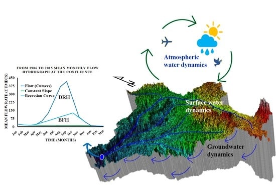
1. Introduction
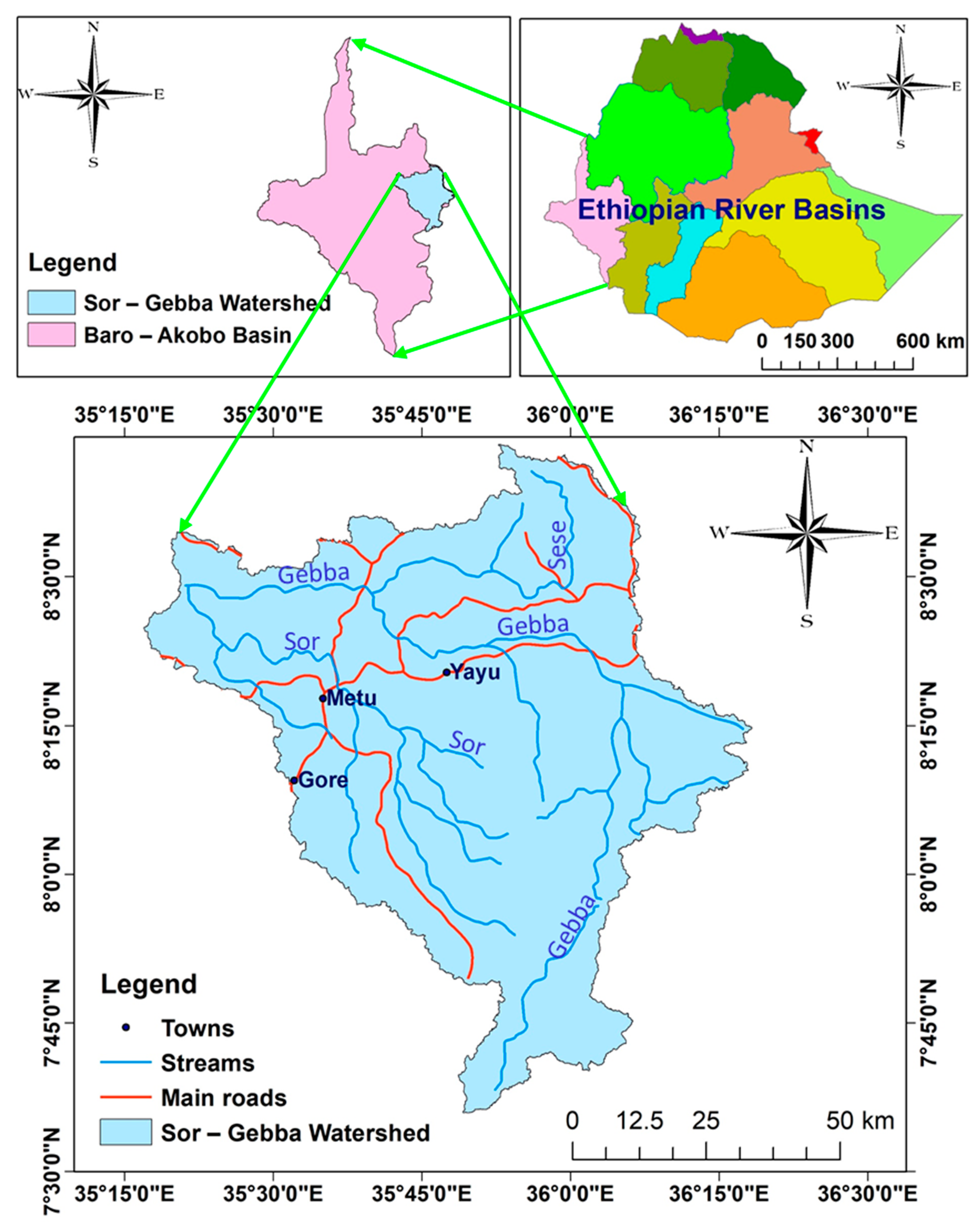
1.1. Description of the Watershed
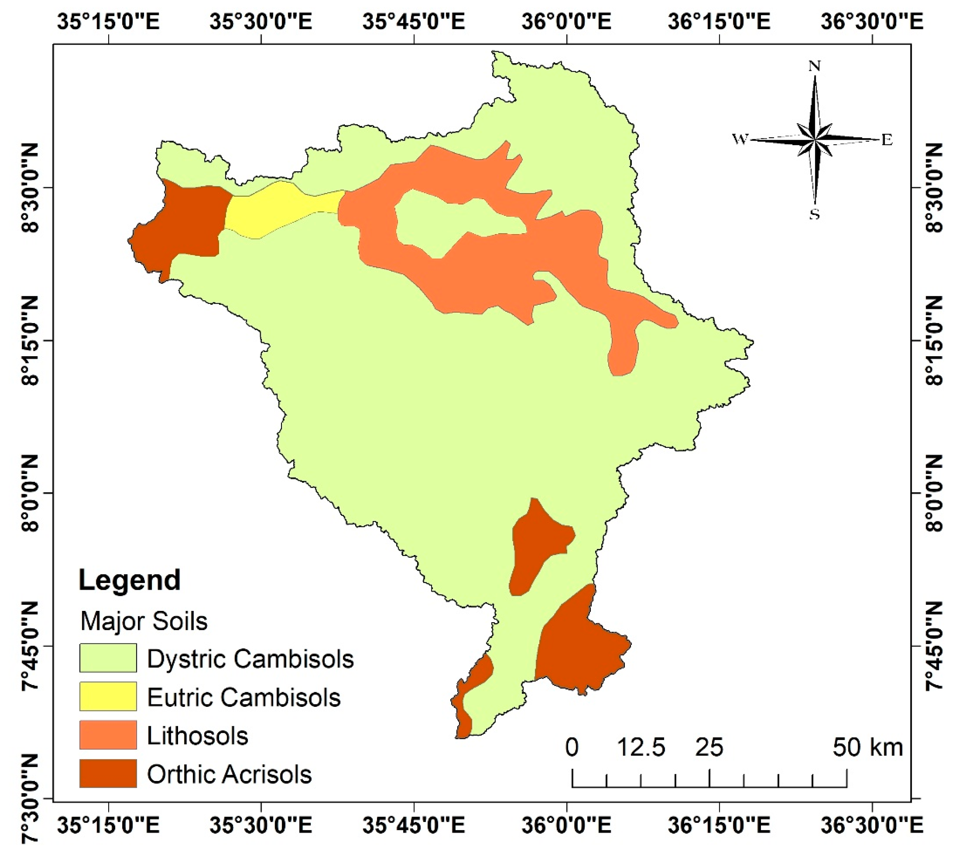
1.2. Physiography and Climate
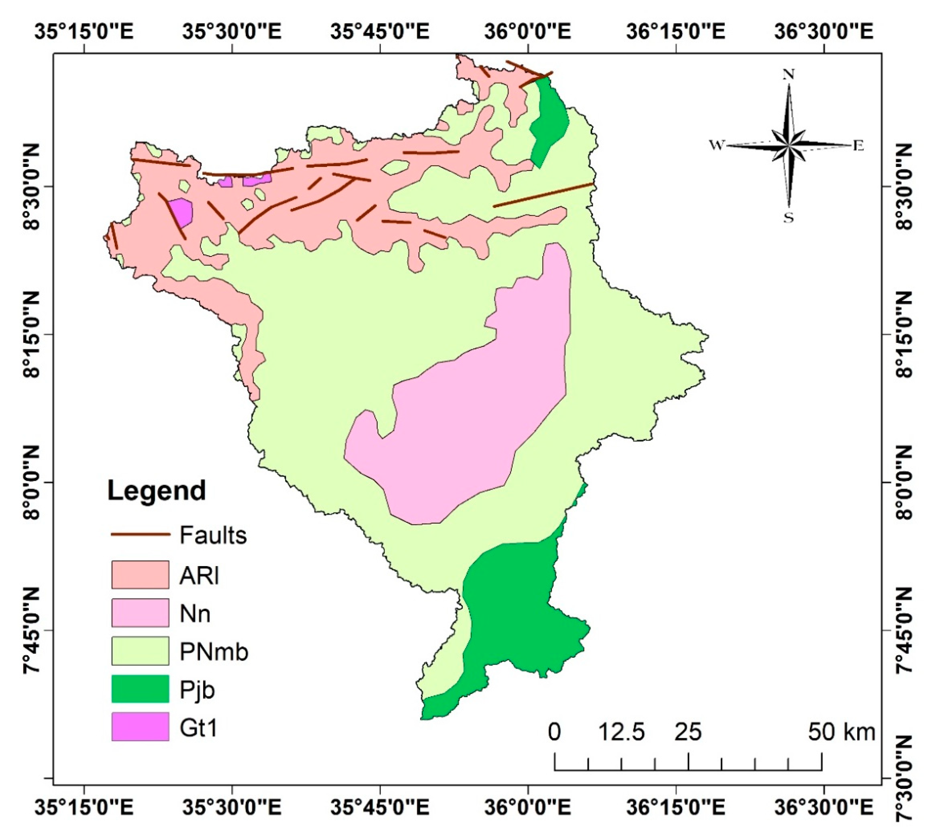
1.3. Geology and Hydrogeology
2. Materials and Methods
2.1. Data Sources, Collection, and Analysis
2.2. Hydrograph and Models Used
3. Results and Discussion
3.1. Manual Hydrograph Analysis
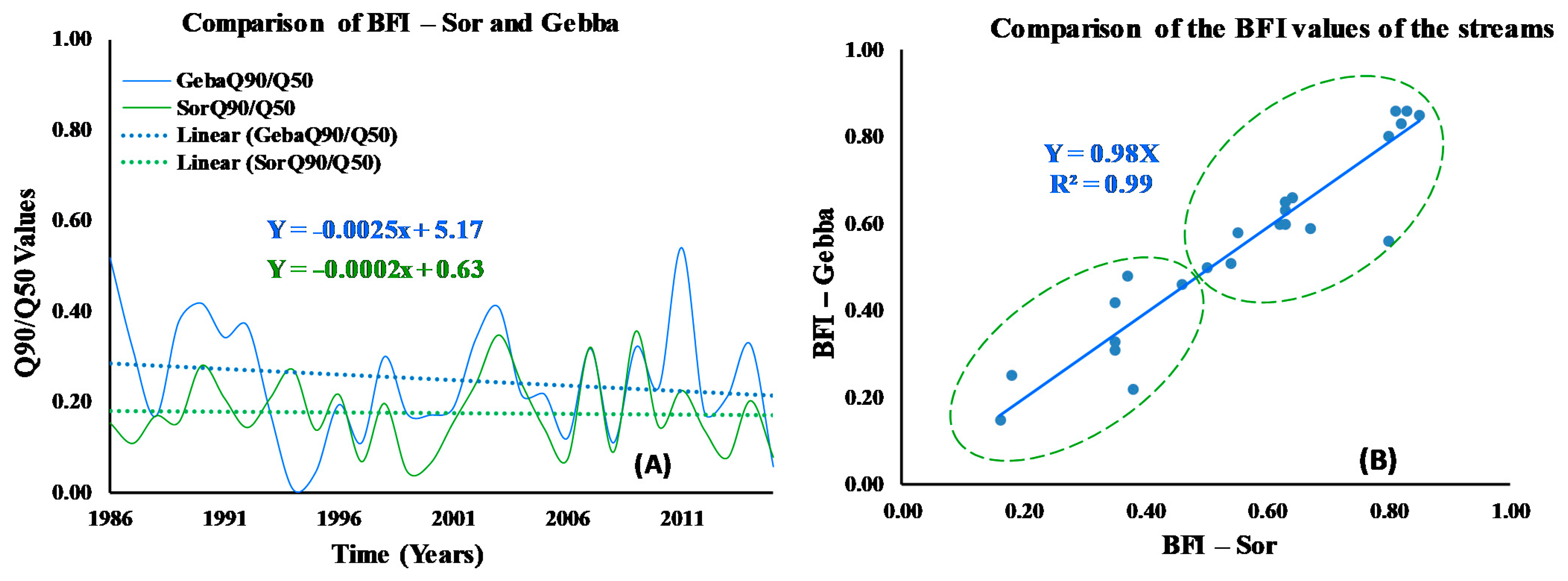
3.2. FDC and BFI
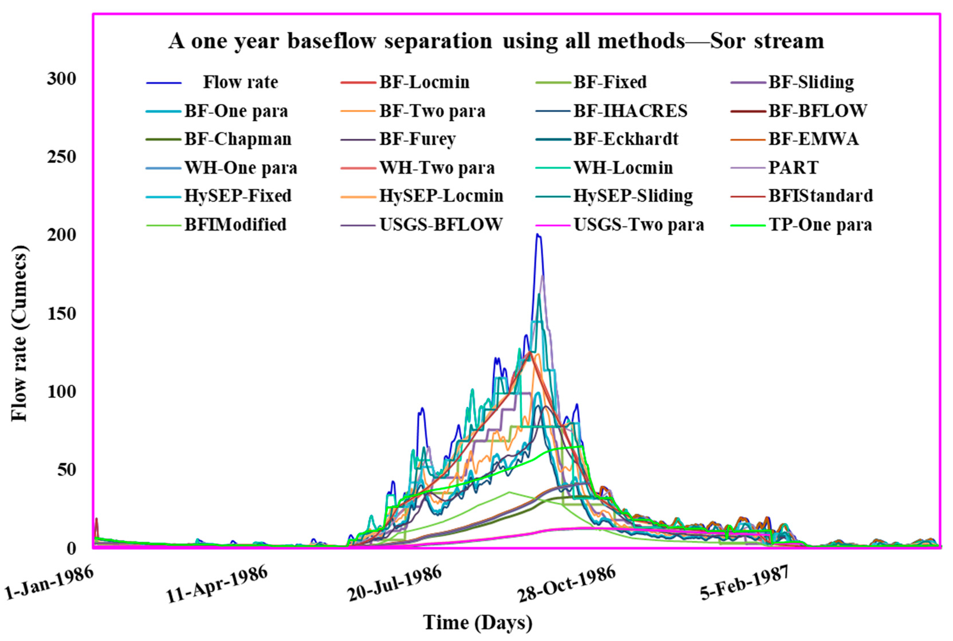
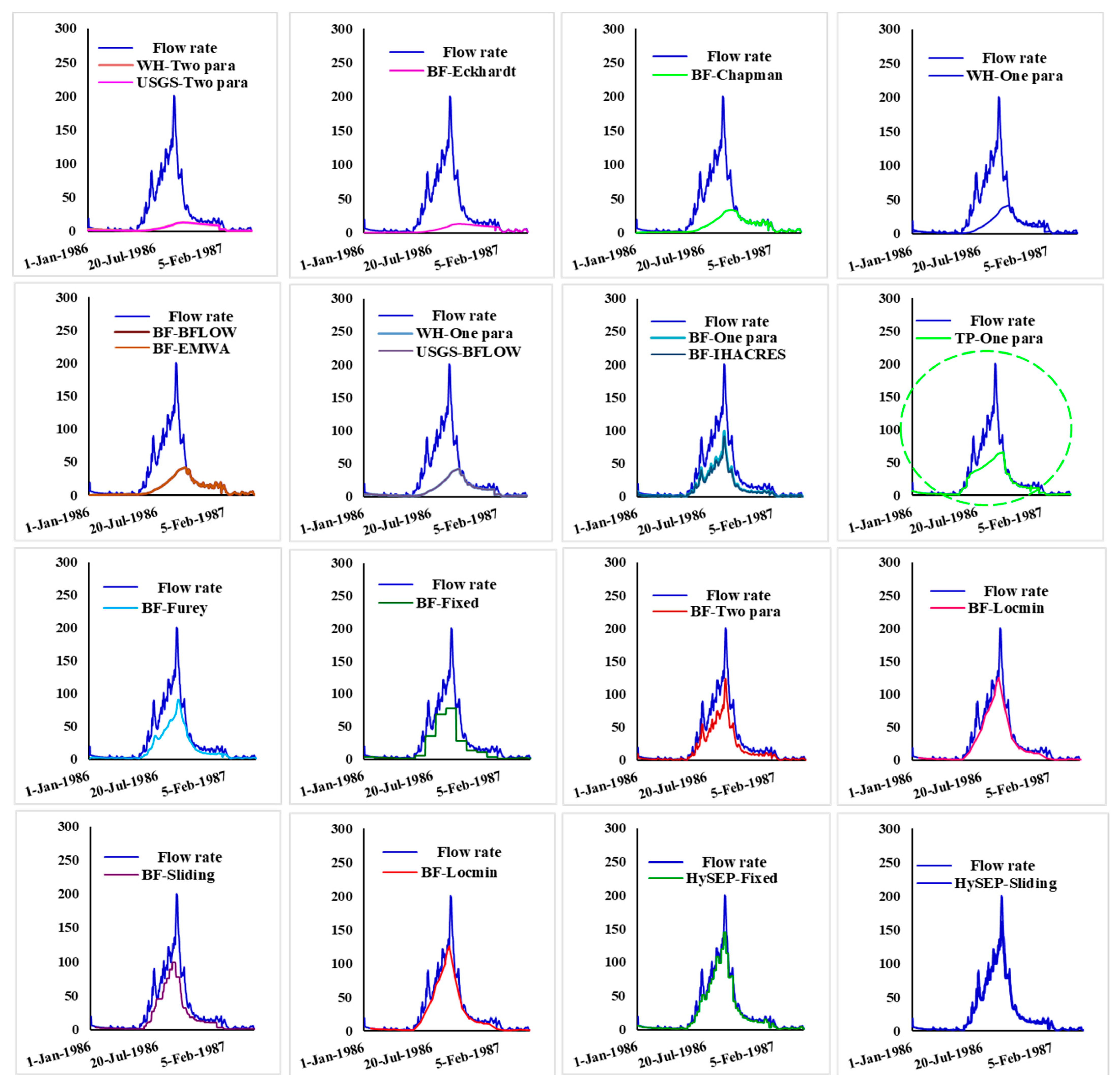
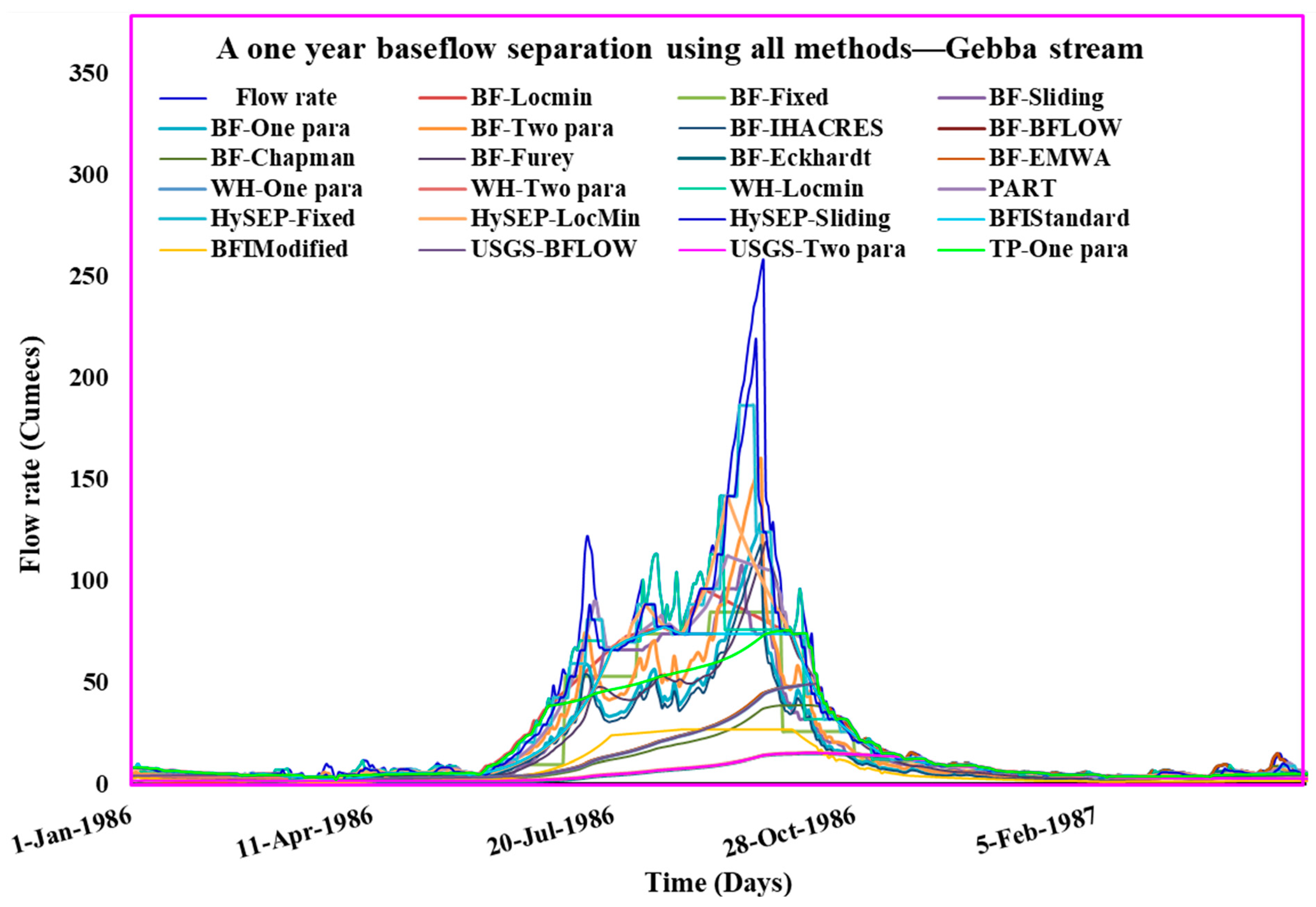
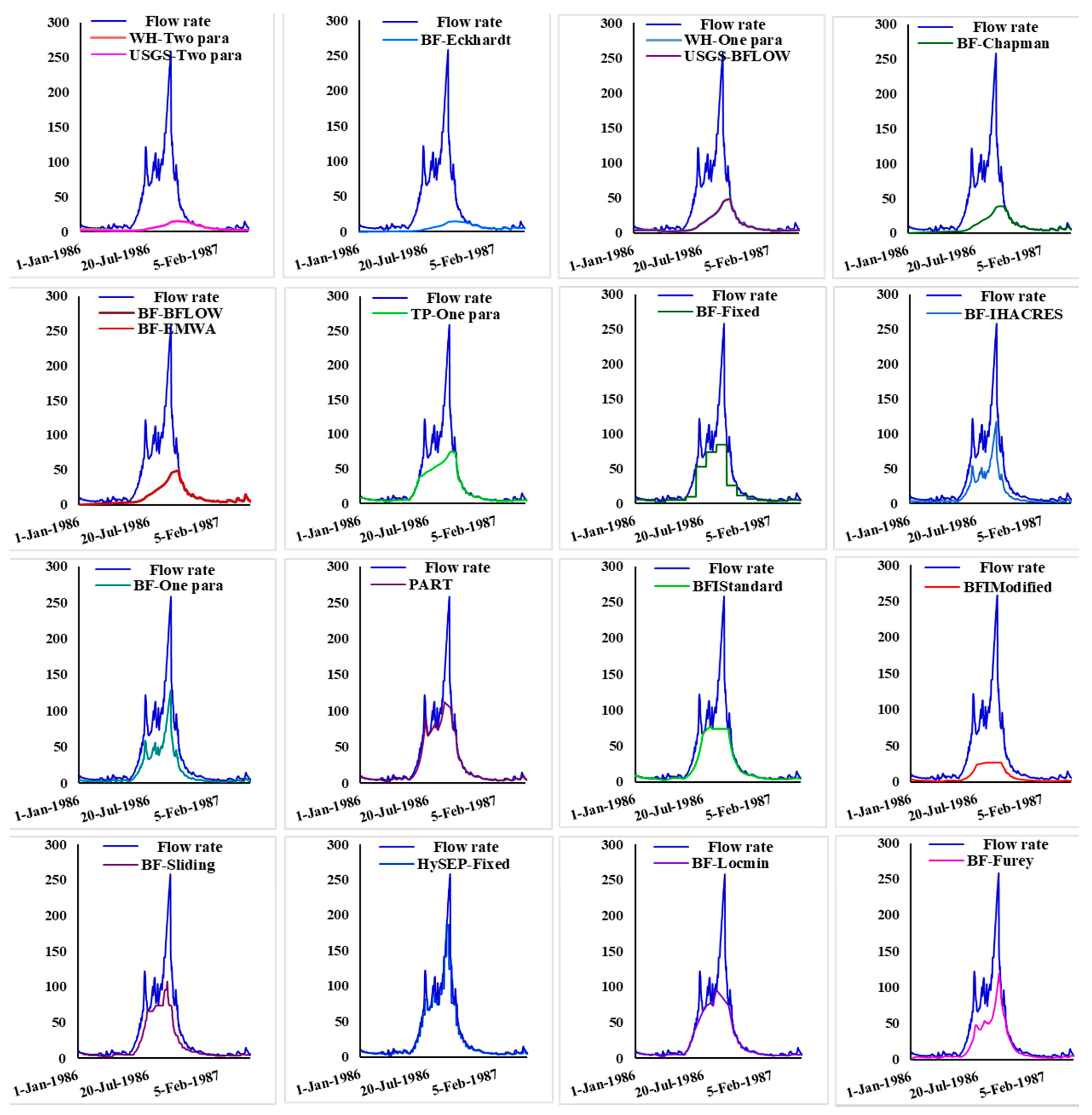
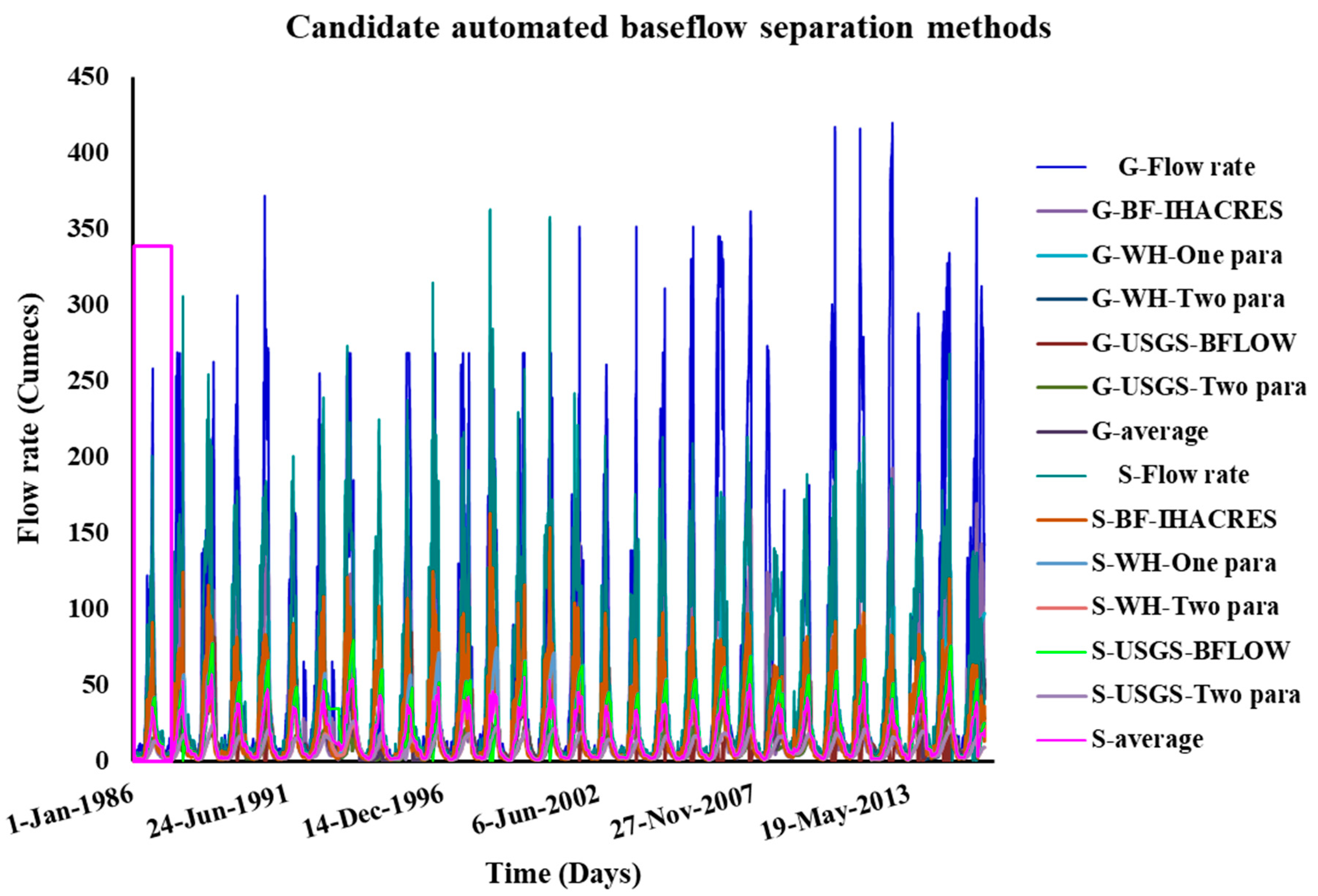
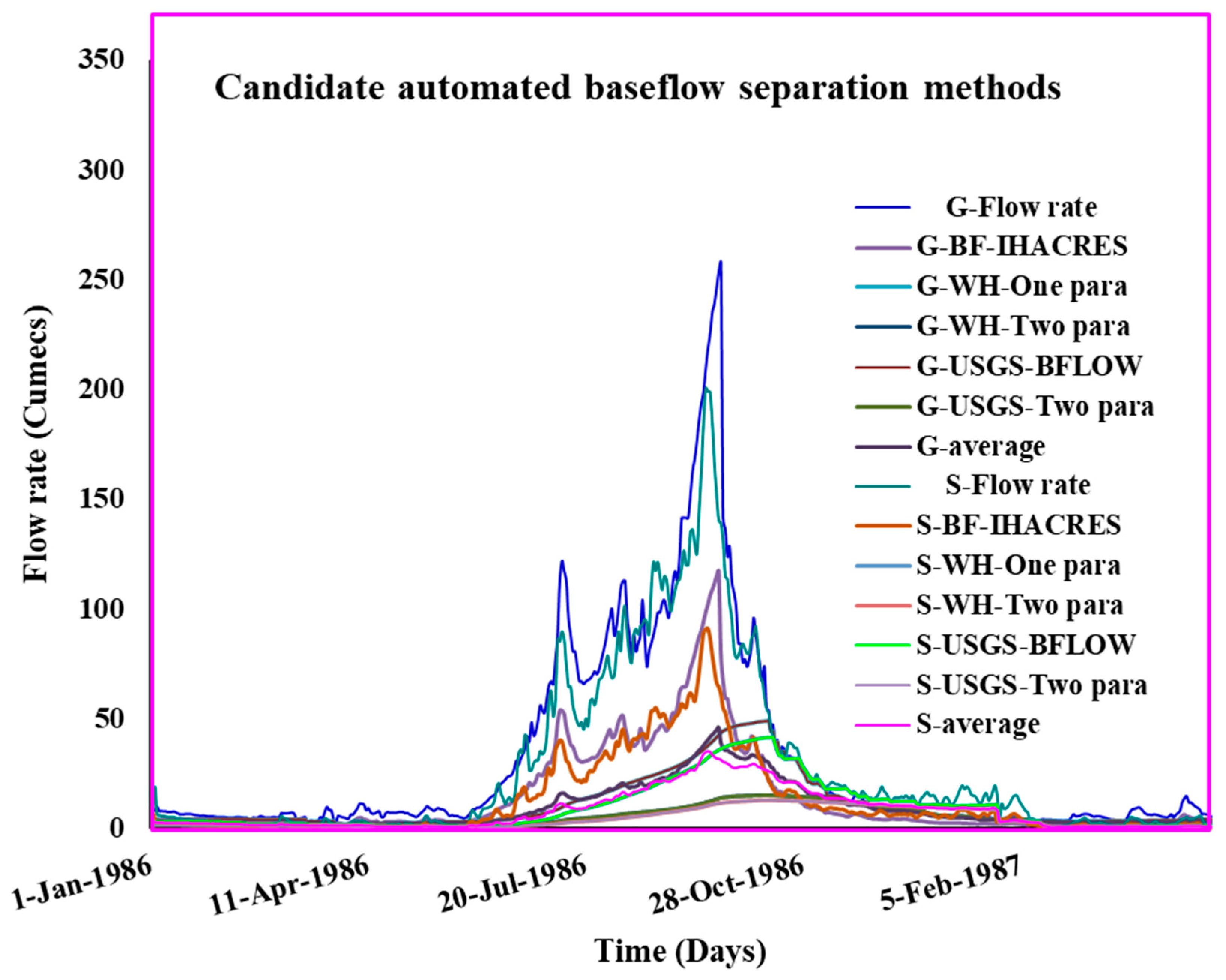
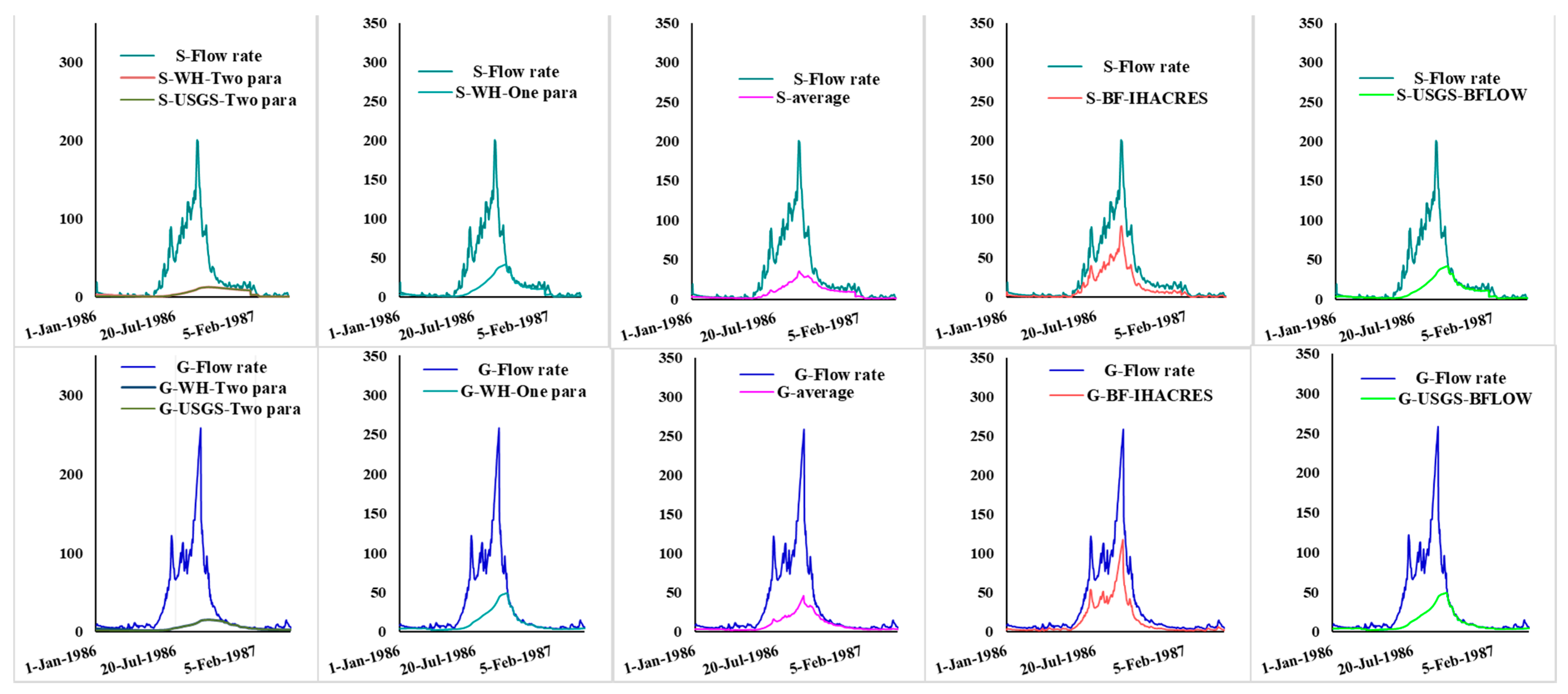
3.3. Automated Baseflow Separation
3.4. Baseflow Separation Using RDF
4. Conclusions
Author Contributions
Funding
Institutional Review Board Statement
Informed Consent Statement
Data Availability Statement
Acknowledgments
Conflicts of Interest
References
- Indarto; Novita, E.; Wahyuningsih, S. Preliminary Study on Baseflow Separation at Watersheds in East Java Regions. Agric. Agric. Sci. 2016, 9, 538–550. [Google Scholar] [CrossRef]
- Viessman, G.L.L.W. Introduction to Hydrology, 4th ed.; Prentice Hall: Upper Saddle River, NJ, USA, 1989; Volume 53, ISBN 9788578110796. [Google Scholar]
- Nathan, R.J.; McMahon, T.A. Evaluation of automated techniques for base flow and recession analyses. Water Resour. Res. 1990, 26, 186. [Google Scholar] [CrossRef]
- Pukh Raj Rakhecha, V.P.S. Applied Hydrometeorology; Capital Publishing Company: New Delhi, India, 2009; Volume 53, ISBN 9788578110796. [Google Scholar]
- Winter, T.C.; Harvey, J.W.; Lehn Franke, O.; Alley, W.M. Groundwater and surface water: A single resource. U.S. Geological Survey Circ. 1139 1998, 17, 37–41. [Google Scholar]
- Boussinesq, J. Recherches theoretique sur l’ecoulement des nappes d’eau infiltrees dans le sol et sur le debit des sources. Pure Appl. Maths 1904, 41, 1–8. [Google Scholar] [CrossRef] [Green Version]
- Maillet, E. Essais d’hydraulique souterraine et fluviale. Nature 1905, 72, 25–26. [Google Scholar]
- Horton, R.E. The Rôle of infiltration in the hydrologic cycle. AGU 1933, 53, 1689–1699. [Google Scholar] [CrossRef]
- Hall, F.R. Base-Flow Recessions—A Review. Water Resour. Res. 1968, 4, 973–983. [Google Scholar] [CrossRef]
- Linsley, R.K.; Kohler, M.A.; Paulhus, J.L.H. Hydrology for Engineers, 3rd ed.; McGraw-Hill: New York, NY, USA, 1982; ISBN 9780070379565. [Google Scholar]
- Zecharias, Y.B.; Brutsaert, W. Recession Characteristics of Groundwater Outflow and Base Flow from Mountainous Watersheds. Water Resour. Res. 1988, 24, 1651–1658. [Google Scholar] [CrossRef]
- Nathan, R.J.; McMahon, T.A. Estimating low flow characteristics in ungauged catchments. Water Resour. Manag. 1992, 6, 85–100. [Google Scholar] [CrossRef]
- Tallaksen, L. A review of baseflow recession analysis. J. Hydrol. 1995, 165, 349–370. [Google Scholar] [CrossRef]
- Gonzales, A.L.; Nonner, J.; Heijkers, J.; Uhlenbrook, S. Comparison of different base flow separation methods in a lowland catchment. Hydrol. Earth Syst. Sci. Discuss. 2009, 13, 34. [Google Scholar] [CrossRef] [Green Version]
- Smakhtin, V.U. Low flow hydrology: A review. J. Hydrol. Hydrol. 2001, 240, 147–186. [Google Scholar] [CrossRef]
- Nathaniel, N. Comparative Analysis of Methods of Baseflow Separation of Otamiri Catchment. Int. J. Sci. Technol. Res. 2017, 6, 314–318. [Google Scholar]
- Jakada, H.; Chen, Z.; Luo, M.; Zhou, H.; Wang, Z.; Habib, M. Watershed characterization and hydrograph recession analysis: A comparative look at a karst vs. non-karst watershed and implications for groundwater resources in Gaolan River basin, Southern China. Water 2019, 11, 743. [Google Scholar] [CrossRef] [Green Version]
- Yang, W.; Xiao, C.; Zhang, Z.; Liang, X. Can the two-parameter recursive digital filter baseflow separation method really be calibrated by the conductivity mass balance method? Hydrol. Earth Syst. Sci. Discuss. 2020, 25, 1–27. [Google Scholar] [CrossRef]
- Scanlon, B.R.; Healy, R.W.; Cook, P.G. Choosing appropriate techniques for quantifying groundwater recharge. Hydrogeol. J. 2002, 10, 18–39. [Google Scholar] [CrossRef]
- Brodie, R.S.; Hostetler, S. A Review of Techniques for Analysing Baseflow from Stream Hydrographs. NZHS-IAH-NZSSS 2005, 28, 13. [Google Scholar]
- Davidson, A. MoWE; MoWE: Ottawa, ON, Canada, 1983; p. 89. [Google Scholar]
- Dingman, S.L. Fluvial Hydraulics; Oxford University Press, Inc.: New York, NY, USA, 2009; Volume 91, ISBN 9788578110796. [Google Scholar]
- Permatasari, R.; Sabar, A.; Natakusumah, D.K.; Samaulah, H. Effects of watershed topography and land use on baseflow hydrology in upstream Komering South Sumatera, Indonesia. Int. J. GEOMATE 2019, 17, 28–33. [Google Scholar] [CrossRef]
- Chernet, T. Hydrogeology of Ethiopia and Water Resouces Development; Ethiopian Institute of Geological Survey, Ministry of Mines and Energy: Addis Ababa, Ethiopia, 1993; p. 227.
- Demlie, M.; Wohnlich, S.; Ayenew, T. Major ion hydrochemistry and environmental isotope signatures as a tool in assessing groundwater occurrence and its dynamics in a fractured volcanic aquifer system located within a heavily urbanized catchment, central Ethiopia. J. Hydrol. 2008, 353, 175–188. [Google Scholar] [CrossRef]
- Alemayehu, T. Determination of Groundwater—Surface Water Interaction and Trans-Boundary Flow. Ph.D. Thesis, Ethiopian Institute of Water Resources, Addis Ababa, Ethiopia, 2016; p. 231. [Google Scholar]
- SELKHOZPROMEXPORT. Baro-Akobo Basin Masterplan Study of Water and Land Resources of the Gambela Plain; SELKHOZPROMEXPORT: Moscow, Russia, 1990; Volume IV, p. 82. [Google Scholar]
- Abbate, E.; Bruni, P.; Sagri, M. Geology of Ethiopia: A Review and Geomorphological Perspectives. Landsc. Landf. Ethiop. 2015, 53, 33–59. [Google Scholar] [CrossRef]
- Geological Survey of Ethiopia. GSE Geology of Ethiopia; Geological Survey of Ethiopia: Addis Ababa, Ethiopia, 2016.
- Tesema, Z. Report on Water well Drilling Site Selection in Yayu Coal Field, Southwestern Ethiopia; Geological Survey of Ethiopia: Addis Ababa, Ethiopia, 2003; p. 11.
- Kazmin, V.; Warden, A.J. Explanation of the Geological Map of Ethiopia; Geological Survey of Ethiopia: Addis Ababa, Ethiopia, 1975; p. 18.
- Ilubabor Zone Water Resources Office. Water supply study document. Unpubl. Rep. 2012, 53, 1689–1699. [Google Scholar]
- Ayenew, T.; Demlie, M.; Wohnlich, S. Hydrogeological framework and occurrence of groundwater in the Ethiopian aquifers. J. African Earth Sci. 2008, 52, 97–113. [Google Scholar] [CrossRef]
- Asfaw, B.; Abaire, B.; Tefera, G. Hydrogeological Report of Gore Area (NC36-16); Ethiopian Institute of Geological Survey: Addis Ababa, Ethiopia, 2001; p. 32.
- Kebede, S. Groundwater in Ethiopia: Features, Numbers and Opportunities; Springer: New York, NY, USA, 2013; ISBN 978-3-642-30391-3. [Google Scholar]
- Mohr, P.A. Mapping of the Major Structures of the African Rift System; Smithsonian Astrophysical Observatory: Cambridge, MA, USA, 1974; p. 70. [Google Scholar]
- Henricksen, B.L.; Ross, S.; Tilimo, S.; Wijntje-Bruggeman, H.Y. Geomorphology and Soils. UNDP; FAO: Rome, Italy, 1984; p. 804. [Google Scholar]
- Driessen, P.; Deckers, J.; Spaargaren, O. Lecture Notes on the Major Soil of the World; FAO: Rome, Italy, 2001; Volume 2006, ISBN 9251046379. [Google Scholar]
- World Meteorological Organization. WMO Guidelines on the Calculation of Climate Normals; World Meteorological Organization: Geneva, Switzerland, 2017; p. 18. [Google Scholar]
- Searcy, J.K. Flow-Duration Curves, Manual of Hydrology: Part 2. Low-Flow Techniques, Methods and practices of the Geological Survey; United States Government Printing Office: Washington, DC, USA, 1969; p. 33.
- Vogel, R.M.; Fennessey, N.M. Flow Duration Curves II. Water Resour. Bull. 1996, 31, 1029–1039. [Google Scholar] [CrossRef]
- Welderufael, W.A.; Woyessa, Y.E. Stream flow analysis and comparison of base flow separation methods: Case study of the Modder River Basin in Central South Africa. Eur. Water 2010, 31, 3–12. [Google Scholar]
- Mohammed, R.; Scholz, M. Flow–duration curve integration into digital filtering algorithms for simulating climate variability based on river baseflow. Hydrol. Sci. J. 2018, 63, 1558–1573. [Google Scholar] [CrossRef] [Green Version]
- Furat, A.M.; Al-Faraj, M.S. Incorporation of the Flow Duration Curve Method Within Digital Filtering Algorithms to Estimate the Base Flow Contribution to Total Runoff. Water Resour. Manag. 2014, 28, 5477–5489. [Google Scholar] [CrossRef]
- Lott, D.A.; Stewart, M.T. Base flow separation: A comparison of analytical and mass balance methods. J. Hydrol. 2016, 535, 525–533. [Google Scholar] [CrossRef]
- Zhang, Y.; Ahiablame, L.; Enge, B.; Liu, J. Regression modeling of baseflow and baseflow index for Michigan USA. Water 2013, 5, 1797–1815. [Google Scholar] [CrossRef] [Green Version]
- Dingman, S.L. Physical Hydrology, 3rd ed.; Waveland Press, Inc.: Long Grove, IL, USA, 2015; ISBN 1478628073. [Google Scholar]
- Freez, R.A.; Cherry, J.A. Groundwater; Prentice-Hall, Inc.: Englewood Cliffs, NJ, USA, 1979; ISBN 0133653129. [Google Scholar]
- Raghunath, H.M. Hydrology (Principles, Analysis and Design), 2nd ed.; New Age International (P) Ltd.: New Delhi, India, 2006; ISBN 9781626239777. [Google Scholar]
- Sloto, R.A.; Crouse, M.Y. Hysep: A Computer Program for Streamflow Hydrograph Separation and Analysis; U.S. Geological Survey: Waterfront Drive Pittsburgh, PA, USA, 1996; p. 54.
- Rutledge, A.T. Development, Analysis, and Application of RORA and PART for Estimating Groundwater Recharge and Discharge in Humid Settings-A Resource for Frequently Asked Questions about the Programs; U.S. Geological Survey: Richmond, VA, USA, 2015; p. 16.
- Piggott, A.R.; Syed Moin, C.S. A revised approach to the UKIH method for the calculation of baseflow. Hydrol. Sci. J. 2005, 50, 911–920. [Google Scholar] [CrossRef]
- Arnold, J.G. Allen Automated Methods for Estimating Baseflow and Groundwater Recharge from Streamflow Records. J. Am. Water Resour. Assoc. 1999, 35, 13353–13366. [Google Scholar] [CrossRef]
- Vincent Lyne, M.H. Stochastic Time-Variable Rainfall-Runoff Modeling; Australian National Conference publication: Perth, Australia, 1979; pp. 89–92. [Google Scholar]
- Price, K. Effects of watershed topography, soils, land use, and climate on baseflow hydrology in humid regions: A review. Prog. Phys. Geogr. 2011, 35, 465–492. [Google Scholar] [CrossRef]
- Eckhardt, K. How to construct recursive digital filters for baseflow separation. Hydrol. Process. 2005, 19, 507–515. [Google Scholar] [CrossRef]
- Chapman, T. A comparison of algorithms for stream flow recession and baseflow separation. Hydrol. Process. 1999, 13, 701–714. [Google Scholar] [CrossRef]
- Mohammed, R.; Scholz, M. Impact of climate variability and streamflow alteration on groundwater contribution to the base flow of the Lower Zab River (Iran and Iraq). Environ. Earth Sci. 2016, 75, 1–11. [Google Scholar] [CrossRef] [Green Version]
- Stewart, M.K. Promising new baseflow separation and recession analysis methods applied to streamflow at Glendhu Catchment, New Zealand. Hydrol. Earth Syst. Sci. 2015, 19, 2587–2603. [Google Scholar] [CrossRef] [Green Version]
- Lim, K.J.; Engel, B.A.; Tang, Z.; Choi, J.; Kim, K.-S.; Muthukrishnan, S.; Tripathy, D. Automated Web GIS based hydrograph analysis tool, WHAT. J. Am. Water Resour. Assoc. 2005, 41, 1407–1416. [Google Scholar] [CrossRef]
- Barlow, P.M.; Cunningham, W.L.; Zhai, T.; Gray, M. U.S. Geological Survey Groundwater Toolbox, a Graphical and Mapping Interface for Analysis of Hydrologic Data (Version 1.0)—User Guide for Estimation of Base Flow, Runoff, and Groundwater Recharge from Streamflow Data; U.S. Geological Survey: Richmond, VA, USA, 2015; p. 27.
- Gregor, M. User’s Manual: BFI+ 3.0. HydrOffice Software Package, Water Science. 2010; Available online: https://hydrooffice.org/Tool/BFI (accessed on 10 May 2021).


| S. No | Zone | Meteorological Station Name | Years of Data | Coordinates (Lat, Lon) | Average Rainfall (mm/year) |
|---|---|---|---|---|---|
| 1 | Ilubabor | Abdela | 1982–1998 | 8°22′, 36°15′ | 1941.01 |
| 2 | Ilubabor | Alge | 1980–1996 | 8°32′, 35°40′ | 1843.70 |
| 3 | Ilubabor | Bilambilo | 2008–2011 | 8°14′, 35°39′ | 1825.43 |
| 4 | Ilubabor | Chora | 2008–2009 | 8°22′, 36°07′ | 1795.33 |
| 5 | Ilubabor | D. Gordomo | 1980–2009 | 7°58′, 35°32′ | 2378.39 |
| 6 | Ilubabor | Darimu/Dipa | 1984–1995 | 8°36′, 36°11′ | 1915.89 |
| 7 | Ilubabor | Dega | 2007–2010 | 8°35′, 36°07′ | 1027.32 |
| 8 | Ilubabor | Fugo leka /Metu | 1967–1997 | 8°18′, 35°35′ | 1833.82 |
| 9 | Ilubabor | Gore | 1953–2010 | 8°09′, 35°32′ | 1801.31 |
| 10 | Ilubabor | Hurumu/Yayu | 1972–2010 | 8°20′, 35°40′ | 1923.27 |
| 11 | Ilubabor | Meligewa | 1987–1995 | 8°24′, 35°31′ | 1748.90 |
| 12 | Ilubabor | Nopha | 1978–1995 | 8°25′, 35°36′ | 1867.42 |
| 13 | Ilubabor | Semodo | 1987–1996 | 8°12′, 35°41′ | 1803.56 |
| 14 | Ilubabor | Sortefasses | 2009 | 8°22′, 35°27′ | 1846.73 |
| 15 | Ilubabor | Suphe | 1980–1995 | 8°30′, 35°39′ | 1587.30 |
| 16 | Ilubabor | Wutete | 2005–2009 | 8°22′, 36°05′ | 1741.45 |
| 17 | Jima | Chira | 1979–1996 | 7°44′, 36°14′ | 1988.91 |
| 18 | Jima | Gatira | 1984–1997 | 7°59′, 36°12′ | 1905.45 |
| Average | 1820.84 | ||||
| Hydrological Stations | Flow (m³/s) | ||||
| 1 | Ilubabor | Sor near Metu (1622 km²) | 1974–2018 | 8°19′, 35°36′ | 51 |
| 2 | Ilubabor | Gebba near Suphe (3894 km²) | 1986–2018 | 8°29′, 35°39′ | 59 |
| 3 | Ilubabor | Sor–Gebba Junction (6556 km²) | Transposition | 8°29′, 35°21′ | 138 |
| Filter Name | Filter Equation | Comments | Source |
|---|---|---|---|
| One parameter algorithm | Chapman and Maxwell (1996) | ||
| Applied as a single pass through the data | |||
| Boughton two-parameter algorithm | Applied as a single pass through the data | Boughton (1993) | |
| Allows calibration against other baseflow | Chapman and Maxwell (1996) | ||
| Information, such as tracers, by adjusting parameter C, | |||
| IHACRES three-parameter algorithm | Extension of Boughton two-parameter algorithm | Jakeman and Hornberger (1993) | |
| Lyne and Hollick algorithm (BFLOW) | ) | α value of 0.925 recommended | |
| for daily stream data filter recommended to be applied in three passes | Lyne and Hollick (1979) Nathan and McMahon (1990) | ||
| Chapman algorithm | ) | Baseflow is | Chapman (1991) Mau and Winter (1997) |
| Furey and Gupta filter | Physically based filter using mass balance equation for baseflow through a hillside | Furey and Gupta (2001) | |
| EWMA filter | Exponential smoothing method of baseflow separation | Tularam & Ilahee (2008) | |
| Eckhardt algorithm | BFImax has three predetermined values for various aquifers as 0.8, 0.5 and 0.25 | Ekhardt (2005) |
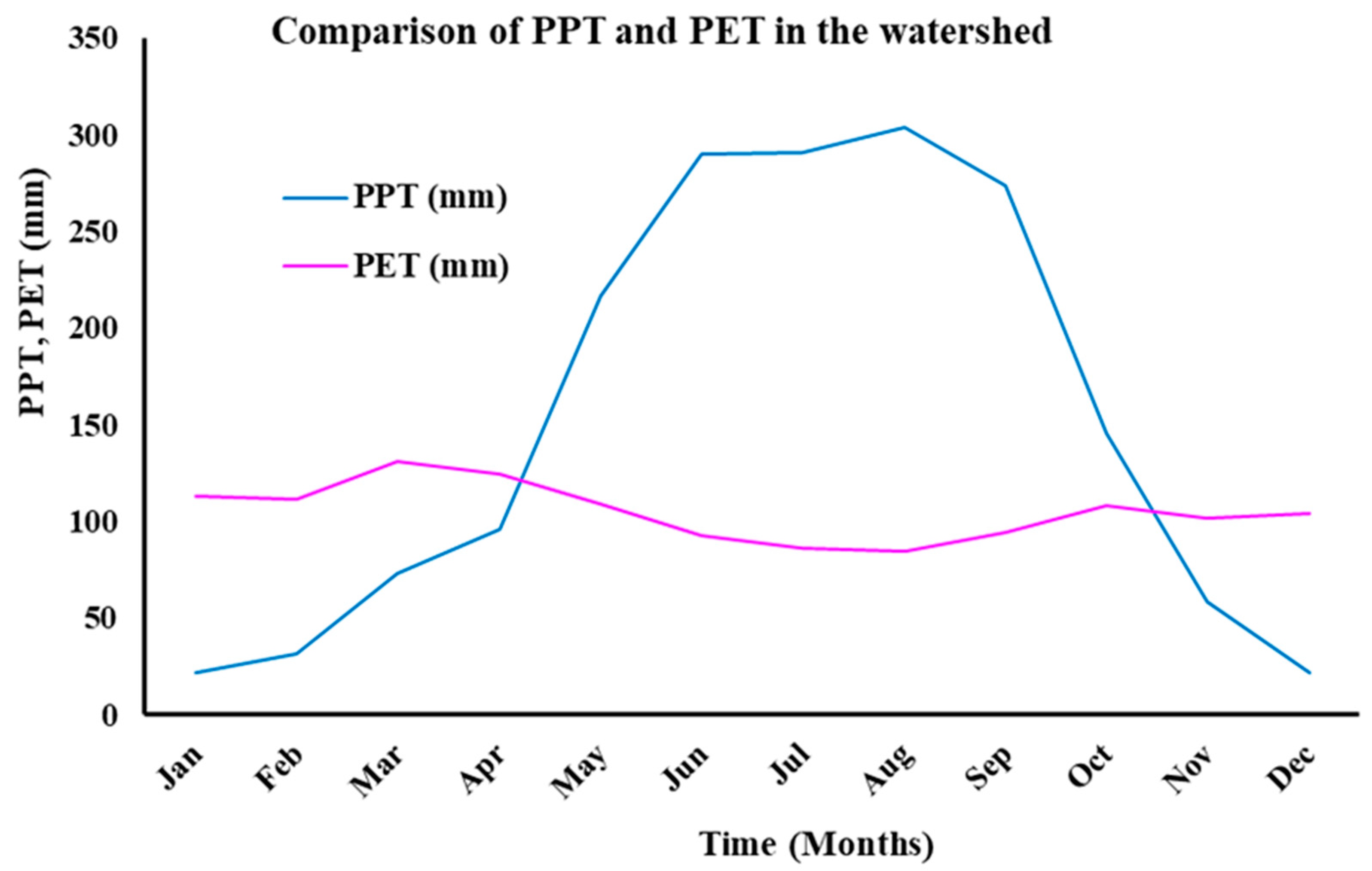
| Months | Jan | Feb | Mar | Apr | May | Jun | Jul | Aug | Sep | Oct | Nov | Dec |
|---|---|---|---|---|---|---|---|---|---|---|---|---|
| PPT (mm) | 22 | 32 | 73 | 96 | 217 | 290 | 291 | 304 | 273 | 146 | 59 | 22 |
| PET (mm) | 113.48 | 111.33 | 131.33 | 124.83 | 109.23 | 92.73 | 86.55 | 84.25 | 94.45 | 108.12 | 101.55 | 104.48 |
| Watershed | Each Year Avg. | All Year Avg. | Manual Avg. | Avg. of Avg. | Area (Km²) | Avg. BFI |
|---|---|---|---|---|---|---|
| Gebba BFI | 0.25 | 0.29 | 0.42 | 0.32 | 3894 | |
| Sor BFI | 0.18 | 0.19 | 0.35 | 0.24 | 1622 | 0.30 |
| Excess Rainfall, d (mm) | DR + Rech = d ∗ A (BCM) | 30% Aquifer Rech (BCM) | Flow @ Confluence (BCM) | Contribution from GW (BCM) |
|---|---|---|---|---|
| 560 | 3.67 | 1.1 | 4.35 | 1.78 |
| 272 | % of baseflow to total streamflow 1.78/4.35 | 0.41 | ||
| S. No | Hydrograph Separation Method | Parameters Used | BFI Values for Sor | BFI Values for Gebba | Avg. BFI Values |
|---|---|---|---|---|---|
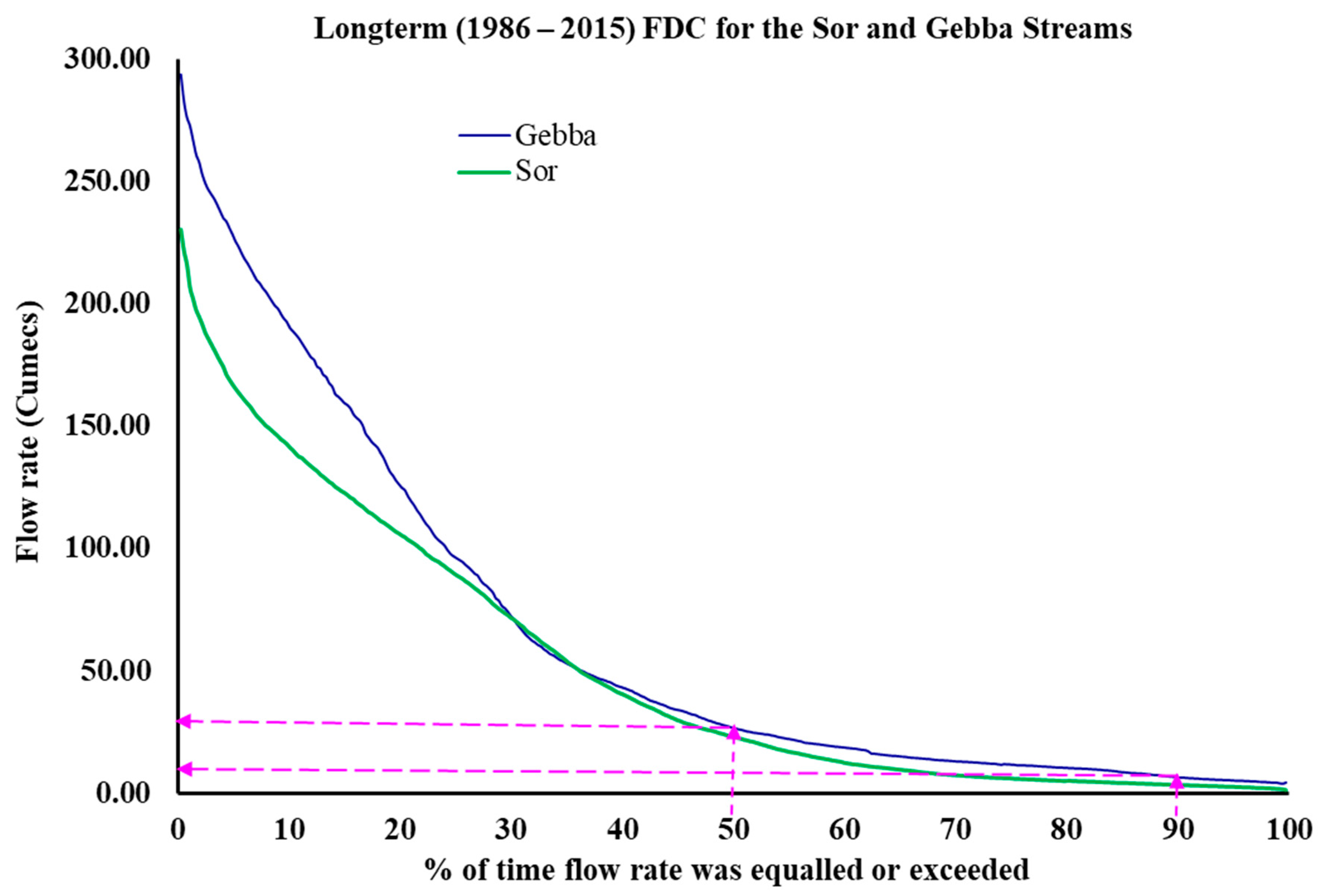
| I | FDC | Q90/Q50 | 0.18 | 0.25 | 0.23 |
| II | Manual Avg. | Recession curve and Graph | 0.35 | 0.42 | 0.40 |
| III | Gabriel Parodi | α = 0.995 | 0.63 | 0.60 | 0.61 |
| IV | WHAT | ||||
| 1 | WH-Locmin | f = 0.9, N = 5 | 0.85 | 0.85 | 0.85 |
| 2 | WH-One para | α = 0.995 | 0.35 | 0.33 | 0.34 |
| 3 | WH-Two para | BFImax = 0.25, C = 0.995 | 0.16 | 0.15 | 0.15 |
| V | HydroOffice (BFI+) | Milos Gregor Model | |||
| 1 | BF-Locmin | f = 0.9, N = 5 | 0.81 | 0.86 | 0.85 |
| 2 | BF-fixed | N = 30 | 0.64 | 0.66 | 0.65 |
| 3 | BF-Sliding | N = 30 | 0.63 | 0.65 | 0.64 |
| 4 | BF-One para | k = 0.4 | 0.50 | 0.50 | 0.50 |
| 5 | BF-Two para | k = 0.4, C = 0.995 | 0.63 | 0.63 | 0.63 |
| 6 | BF-IHACRES | αq = 0.01, C = 0.5, k = 0.4 | 0.46 | 0.46 | 0.46 |
| 7 | BF-BFLOW | α = 0.995 | 0.80 | 0.56 | 0.63 |
| 8 | BF-Chapman | α = 0.995 | 0.67 | 0.59 | 0.61 |
| 9 | BF-Furey | C1 = 0.1, C2 = 0.13, g = 0.05, d = 2 days | 0.62 | 0.60 | 0.61 |
| 10 | BF-Eckhardt | α = 0.995, BFmax = 0.25 | 0.55 | 0.58 | 0.57 |
| 11 | BF-EWMA | α = 0.005 | 0.80 | 0.80 | 0.81 |
| VI | USGS GW Toolbox | ||||
| 1 | HYSEP-Fixed | N = 30 | 0.64 | 0.66 | 0.65 |
| 2 | HYSEP-Locmin | f = 0.9, N = 5 | 0.82 | 0.83 | 0.83 |
| 3 | HYSEP-Sliding | N = 30 | 0.63 | 0.65 | 0.64 |
| 4 | PART | 0.83 | 0.86 | 0.85 | |
| 5 | USGS-One para | α = 0.995 | 0.35 | 0.31 | 0.32 |
| 6 | USGS-Two para | α = 0.995, BFmax = 0.25 | 0.37 | 0.48 | 0.45 |
| 7 | BFI-Standard | k = 0.9, N = 5 | 0.54 | 0.51 | 0.52 |
| 8 | BFI-Modified | k′ = 0.995, N = 30 | 0.38 | 0.22 | 0.27 |
| min | 0.16 | 0.15 | 0.15 | ||
| max | 0.85 | 0.86 | 0.85 | ||
| avg | 0.57 | 0.56 | 0.56 |
| S. No | Hydrograph Separation Method | Parameters Used | BFI Values for Sor | BFI Values for Gebba | Avg. BFI Values |
|---|---|---|---|---|---|
| I | FDC | Q90/Q50 | 0.18 | 0.25 | 0.23 |
| II | Manual Avg. | Recession curve and graph | 0.35 | 0.42 | 0.40 |
| III | WHAT | ||||
| 1 | RDF-One parameter | α = 0.995 | 0.35 | 0.33 | 0.34 |
| 2 | RDF-Two parameters | BFImax = 0.25, C = 0.995 | 0.16 | 0.15 | 0.15 |
| IV | HydroOffice | Milos Gregor model | |||
| 1 | RDF-IHACRES | αq = 0.01, C = 0.5, k = 0.4 | 0.46 | 0.46 | 0.46 |
| V | USGS GW Toolbox | ||||
| 1 | RDF-One parameter | α = 0.995 | 0.35 | 0.31 | 0.32 |
| 2 | RDF-Two parameters | α = 0.995, BFImax = 0.25 | 0.37 | 0.48 | 0.45 |
| 3 | BFI-Modified | k′ = 0.995, N = 30 | 0.38 | 0.22 | 0.27 |
| min | 0.16 | 0.15 | 0.15 | ||
| max | 0.46 | 0.48 | 0.46 | ||
| avg | 0.33 | 0.33 | 0.33 |
Publisher’s Note: MDPI stays neutral with regard to jurisdictional claims in published maps and institutional affiliations. |
© 2021 by the authors. Licensee MDPI, Basel, Switzerland. This article is an open access article distributed under the terms and conditions of the Creative Commons Attribution (CC BY) license (https://creativecommons.org/licenses/by/4.0/).
Share and Cite
Bayou, W.T.; Wohnlich, S.; Mohammed, M.; Ayenew, T. Application of Hydrograph Analysis Techniques for Estimating Groundwater Contribution in the Sor and Gebba Streams of the Baro-Akobo River Basin, Southwestern Ethiopia. Water 2021, 13, 2006. https://doi.org/10.3390/w13152006
Bayou WT, Wohnlich S, Mohammed M, Ayenew T. Application of Hydrograph Analysis Techniques for Estimating Groundwater Contribution in the Sor and Gebba Streams of the Baro-Akobo River Basin, Southwestern Ethiopia. Water. 2021; 13(15):2006. https://doi.org/10.3390/w13152006
Chicago/Turabian StyleBayou, Wondmyibza Tsegaye, Stefan Wohnlich, Mebruk Mohammed, and Tenalem Ayenew. 2021. "Application of Hydrograph Analysis Techniques for Estimating Groundwater Contribution in the Sor and Gebba Streams of the Baro-Akobo River Basin, Southwestern Ethiopia" Water 13, no. 15: 2006. https://doi.org/10.3390/w13152006