
Search Space Reduction for Genetic Algorithms Applied to Drainage Network Optimization Problems
by
 , , and
Leonardo Bayas-Jiménez
1,* ,
,
F. Javier Martínez-Solano
1 ,
,
Pedro L. Iglesias-Rey
1 and
and
Daniel Mora-Meliá
2 1
Department of Hydraulic Engineering and Environment, Universitat Politècnica de València, Camino de Vera s/n, 46022 Valencia, Spain
2
Department of Engineering and Construction Management, Faculty of Engineering, Universidad de Talca, Camino Los Niches Km 1, Curicó 3340000, Chile
*
Author to whom correspondence should be addressed.
Water 2021, 13(15), 2008; https://doi.org/10.3390/w13152008
Submission received: 4 June 2021
/
Revised: 15 July 2021
/
Accepted: 17 July 2021
/
Published: 22 July 2021
(This article belongs to the Special Issue Urban Hydraulic Engineering Simulation and Calculation)
Abstract
:In recent years, a significant increase in the number of extreme rains around the world has been observed, which has caused an overpressure of urban drainage networks. The lack of capacity to evacuate this excess water generates the need to rehabilitate drainage systems. There are different rehabilitation methodologies that have proven their validity; one of the most used is the heuristic approach. Within this approach, the use of genetic algorithms has stood out for its robustness and effectiveness. However, the problem to be overcome by this approach is the large space of solutions that algorithms must explore, affecting their efficiency. This work presents a method of search space reduction applied to the rehabilitation of drainage networks. The method is based on reducing the initially large search space to a smaller one that contains the optimal solution. Through iterative processes, the search space is gradually reduced to define the final region. The rehabilitation methodology contemplates the optimization of networks using the joint work of the installation of storm tanks, replacement of pipes, and implementation of hydraulic control elements. The optimization model presented uses a pseudo genetic algorithm connected to the SWMM model through a toolkit. Optimization problems consider a large number of decision variables, and could require a huge computational effort. For this reason, this work focuses on identifying the most promising region of the search space to contain the optimal solution and to improve the efficiency of the process. Finally, this method is applied in real networks to show its validity.
1. Introduction
Drainage systems around the world have experienced an increase in operating pressure in recent years. This is mainly due to the increase in the intensity of rains and urban growth. According to many authors, extreme rains occur with increasing frequency around the world, mainly due to climate change, and are the main factor of flooding in urban basins [1,2,3]. On the other hand, anthropological action has altered the composition of the world atmosphere; one of the most evident is produced by the development of urban space. During the last few decades, cities have experienced a constant process of growth, which has reduced the green areas that surround them, replacing them with highly impermeable surfaces. These factors have led many cities to appreciate the increase in surface runoff, and in many cases, the collapse of their drainage systems [4,5,6]. These problems make it necessary to improve the functioning of the drainage networks to restore security to the cities. Floods in urban areas generate significant economic impacts in cities. Concern increases as cities are increasingly exposed to flood risk [7,8]. To face this problem, different options for optimizing drainage networks have been developed.
One of the most prominent approaches is called low impact development (LID). LID approaches have been widely used to minimize the flow of water produced by urban runoff, retaining the water and enhancing its infiltration. This type of approach also attempts to improve water quality by removing pollutants in vegetation and restoring urban ecosystems. Among the most used types of these systems are permeable paving, infiltration trenches, vegetated swales, bio retention basins, and infiltration basins. However, although LIDs are a valid solution to reduce runoff, these approaches do not have great resilience in extreme rain events [9,10,11,12]. The use of storm tanks in an urban environment to reduce the risk of flooding has been studied and proven as one of the most efficient methods to reduce surface runoff [13,14,15]. Better results have been given by using the combination of storm tank installation and pipe renewal [16,17]. The inclusion of hydraulic control elements [18] appear as an improvement of these works, and turns out to be an alternative that improves the results obtained.
To face the problem of floods, some authors improved the networks by taking as a criterion the avoidance of floods in the study area [19], while other authors improved the networks based on the flood volume [16,20]. Different methodologies have been developed to address this problem. However, the need to find minimal cost designs has led researchers to optimization algorithms. Different evolutionary techniques have been tested for the optimization of drainage networks, highlighting an ant colony optimization algorithm [21,22], simulated annealing [15,23], harmony search algorithm [24,25], and taboo search algorithm [26]. All of these techniques show good results in different cases studied. However, genetic algorithms that do not require continuity of the objective function stand out in this field due to their robustness, and their use has gained popularity in drainage network optimization work [10,16,17,27,28,29,30].
Genetic algorithms are stochastic search strategies based on natural selection mechanisms, which involve aspects of biological evolution to solve optimization problems. One characteristic of these types of algorithms is the way that they explore the space solution. While other algorithms follow a single search direction, genetic algorithms perform parallel searches in different directions. This characteristic adds to their ability to explore complex adaptive landscapes, and has made these algorithms a widely used tool in water resources research.
However, one of the problems that most worries researchers is the difficulty that genetic algorithms (GAs) can present in finding solutions close to the global optimum. Kadu et al. [31] mentions that genetic algorithms are efficient and effective in finding low-cost solutions in drainage system optimization problems. The efficiency and effectiveness depend on several parameters, some that contemplate the parameters of the algorithm and others of the space where the GA seeks the optimal solutions. The problem with the search space (SS) occurs because of the large number of decision variables (DVs) that the algorithm must analyze in a real-life problem. Handling a significant number of DVs causes the SS to grow exponentially. This problem turns into a considerable computational demand to find a satisfactory solution to the problem proposed. Although the computational advance can compensate the time required in this operation, in reality, there are problems in which the SS is so large that it becomes unapproachable. For this reason, the need arises to reduce the SS. This reduction, however, must be done in such a way that the most promising region that contains the best solutions is clearly identified. Maier et al. [32] mention that a reduction in the size of the SS generally results in its approximation, either because a series of DVs have to be fixed before optimization or because the nature of the interactions between the DVs excludes the effective size reduction. This could potentially exclude the region containing the global optimum, and thus reduce the quality of the solutions found. For this reason, the reduction method must guarantee that the selected region is truly the best, and that the best solutions to the problem are not excluded from it. To solve this situation, different works have been carried out to effectively reduce the SS.
One of the first works was carried out by Schraudolph and Belew [33]. These authors presented an approach based on dynamic parameter coding to adaptively control the mapping of fixed-length chromosomes to real values, so that, at each iteration, the algorithm searches a smaller SS. Ndiritu and T.M. Daniell [34] presented a modified GA combining a fine-tuning strategy to reduce the SS with a hill climbing strategy to move to more promising regions. In recent research, Sophocleous, Savić, and Kapelan [35] presented a model to detect and locate leaks in water distribution networks. The model employs two stages: search space reduction, and leak detection and location. In the first stage, they reduce the number of DVs and the range of values that they can take through an analysis of the characteristics of the network. For the second stage, they used a GA to find the solution to the problem. Simultaneously, Ngamalieu-Nengoue, Iglesias-Rey, and Martínez-Solano presented a methodology to search space reduction (SSR) applied to a drainage network rehabilitation model. The reduction of the SS is based on locating the possible nodes in which storm tanks (STs) will be installed and subsequently identifying the possible pipes that should be renewed. The process is carried out by reducing the number of DVs and the range of values that they can adopt. In a later work Bayas-Jiménez et al. [18], they used the same methodology to optimize drainage networks. The authors included in the optimization process the use of hydraulic controls that certainly improved the results obtained, but that considerably increased the SS. The proposed methodology continues and complements these works with the aim of improving the efficiency of the optimization process. Specifically, the method reduces the SS using the sectorization criteria to improve calculation times and reduce the computational effort required. To achieve this, an SSR method is applied in each hydraulic sector, decreasing the DVs and defining a final search region. Once the region that is presumed to have the best solutions is delimited, a final optimization is carried out to find the best possible solution. The method is applied to different drainage networks to prove its benefits.
2. Materials and Methods
2.1. Problem Statement
This work consists of the rehabilitation of networks that present flood problems due to lack of capacity. To improve the network, the renovation of pipes for others of greater capacity, the installation of STs, and the installation of HCs were considered. In the optimization model, the possible diameters of the pipes to be renewed, the volume of the storage of the STs, and the degrees of opening of the control element were defined as DVs. For use in the optimization model, they must be fully defined. The first type of DV consists of all pipes in the network NC; each of these pipes can take a diameter value from a previously defined list of options ND. If a DV takes the value of 0, it indicates that this pipe does not need to increase its diameter, while a different value indicates that this pipe was optimized by the optimization model. The group of optimized DVs is represented by the notation ms. A second group of DVs consist of all nodes of the NN network where STs can be installed. As these DVs represent the volume required by each ST, for the analysis, the maximum height of the tank equal to the current height of the manhole is considered, leaving the cross-sectional area of the tank as a variable. This DV can take values within an options list NS defined in the discretization of the cross-sectional area of the tank. If, in the optimization process, the value 0 is obtained for a DV, it must be understood that this node does not require an ST to be installed. The set of nodes that requires STs to be installed is represented by the notation ns. Finally, the third group of DVs consists of the decision variables that determine the installation of HCs in the pipes. This group of DVs can take values from a list of options Nθ that results from discretizing the degree of opening. The value 0 indicates that the installation of an HC is not necessary. The group of optimized DVs is represented by the notation ps.
2.2. Optimization Model
The optimization model in this article considered the methodology presented in a previous work [18]. The model used as an optimization engine a modified genetic algorithm called the pseudo genetic algorithm (PGA) [36]. Genetic algorithms are inspired by the theory of evolution and natural selection. GAs work on a set of potential solutions called the population. This population is composed of a series of solutions called individuals, and an individual is made up of a series of positions that represent each of the DVs involved in the optimization processes, which are called chromosomes. These chromosomes are made up of a string of numbers called coding. A traditional GA has a binary coding. In contrast, the PGA used in this work has an integer coding. This coding has the advantage that each gene represents a DV that gives good results in optimization of hydraulic problems. In a GA, each individual is defined as a data structure that represents a possible solution of the SS of the problem. Evolution strategies work on individuals, who represent solutions to the problem, so they evolve through generations. Within the population, each individual is differentiated according to their value of the objective function. To obtain the next generations, new individuals are created using two basic evolution strategies, such as the crossover operator and the mutation operator.
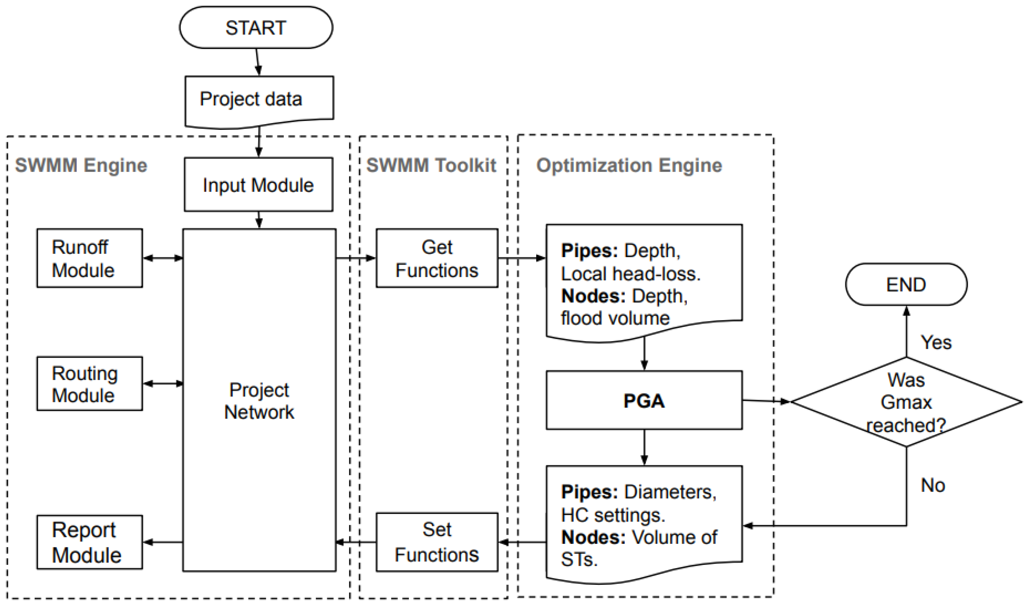
The PGA connects to the SWMM model [37] using a toolkit [38] to carry out a series of simulations in order to find an optimal solution to the problem. To achieve this, the PGA evaluates an objective function composed of four cost functions [18] that are determined based on the results provided by the storm water management model (SWMM) in the simulations carried out. This process is carried out iteratively until a defined stop criterion is reached. Figure 1 summarizes the operation of the optimization model.
This optimization process is iterative, and requires establishing an end point to the process. GAs end the process when a high percentage of the population converges to a value or a fixed number of evaluations that is determined by criteria, such as a maximum number of generations or a maximum resolution time. In this work, the termination criterion was based on the value of the objective function. When, after a certain number of generations (), the OF does not decrease, the algorithm stops. At that time, it is understood that the solution will not improve, and the process ends.
2.2.1. Objective Function
The optimization problem aims to minimize the costs associated with flood damage with as little investment as possible. According to this, an objective function is established that evaluates the problem in economic terms. This objective function consists of four cost functions. The first function corresponds to the cost of the renewal of pipes that must be replaced due to the lack of capacity. This function is established from actual cost data provided by pipe manufacturers. The function relates the cost of the pipe to its diameter. In addition, it includes the coefficients α and β to adjust the cost according to the place where the methodology is applied.
In Equation (1), Di is the diameter of the pipe, Li is the length of the pipe, and the coefficients α and β are adjustment coefficients selected for a specific project.
The second term corresponds to the cost of installing STs that would be required to temporarily store the water that the network is not able to evacuate in the event of extreme rain.
The first term of Equation (2) represents a minimum cost (Cmin) established for the construction of the STs, while the second term is a variable as a function of the required storage volume (Vi) affected by a constant Cvar and an exponent ω.
The third term of the objective function represents the cost of installing HC elements in certain pipes at the outlet of STs. This function is established from actual gate valve cost data.
In Equation (3), Di is the diameter of the pipe, and the coefficients γ and μ are used to adjust the cost of the HC elements to the place where the methodology is applied.
Finally, an equation must be defined that presents the cost of flood damage; this function depends on the level reached by the water yi. The definition of this cost is based on the work done by Ngamalieu-Nengoue et al. [16]. The authors combined this curve with the costs of flooding per square meter for different land uses. In Equation (4), from 1.40 m of flooding, the damage is considered irreparable and, therefore, the function stops growing, and the cost will reach its maximum (Cmax). Then, a constant ymax equal to 1.40 m is established.
These four cost functions define the objective function (Equation (5)) that the optimization model will seek to decrease to reach the best solution.
2.2.2. PGA Parameters
For an adequate work of the algorithm, a suitable population size must be defined, so that, on the one hand, the SS of the analyzed scenario is adequately covered and, on the other hand, it does not demand excessive computational effort. An expression (Equation (6)) is defined to face the problem efficiently. The equation was presented in a work developed by Mora-Melia et al. [36].
where N represents the population, NDV represents the number of DVs, and ϕ is a constant with a value equal to 2. To give the model an element of diversity, a mutation probability is defined, which is established in Equation (7) by Mora-Melia et al. in a previous work [36].
where δ is a constant with a value equal to 1.
The optimization model uses a stop criterion Gmax presented by Bayas-Jiménez et al. [18] and shown in Equation (8).
where Pe is called the probability of success, which is defined according to the requirement of the calculation to be performed. After several runs, the authors have concluded that a value of Pe of 80% is needed to guarantee a change due to mutation, however, in this work, different percentages were used according to the different scenarios proposed. Finally, PO is the probability of occurrence that is determined using Equation (9).
where NDV is the number of DVs that have been analyzed, Xmax is the maximum number of discretization options for the DVs, and Pmut is the mutation probability.
2.3. Search Space Reduction Process
Transforming the SS from continuous to discrete inherently leads to a problem. If the discretization is small, that is, the number of options that the DV can take is small, then the space exploration may not be efficient, and the algorithm may not be able to identify an optimal solution. On the other hand, if the discretization is very refined, the list of options that the DV can take would notably increase the SS, and the computational effort required would be considerable. The SS is defined considering the DVs and the values that these can adopt; an expression is then defined (Equation (10)) that allows us to know the size of SS that the algorithm must explore in each proposed scenario.
where ni represents the candidate pipes to be renewed, mi represents the candidate nodes to install STs, and pi represents the candidate pipes to install HCs in a defined scenario. The equation is presented in logarithmic form with the aim that the SS can be appreciated in a better way.
2.3.1. Reduction by Hydraulic Sectors
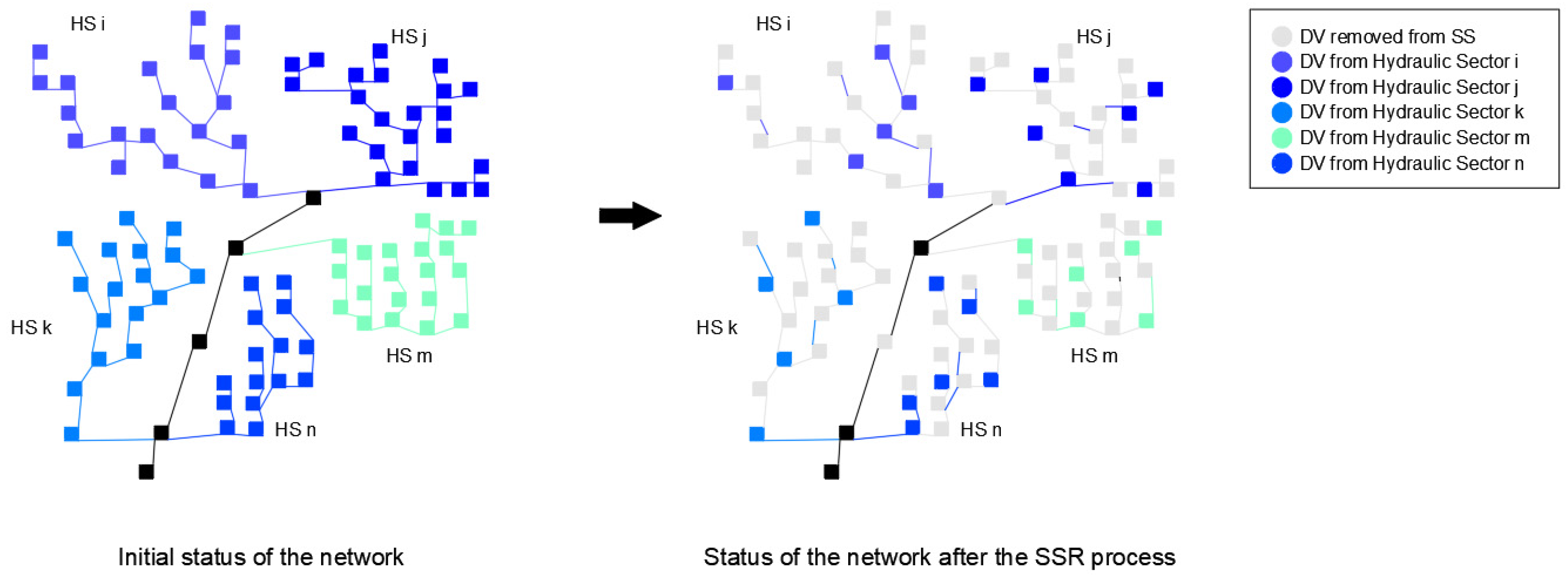
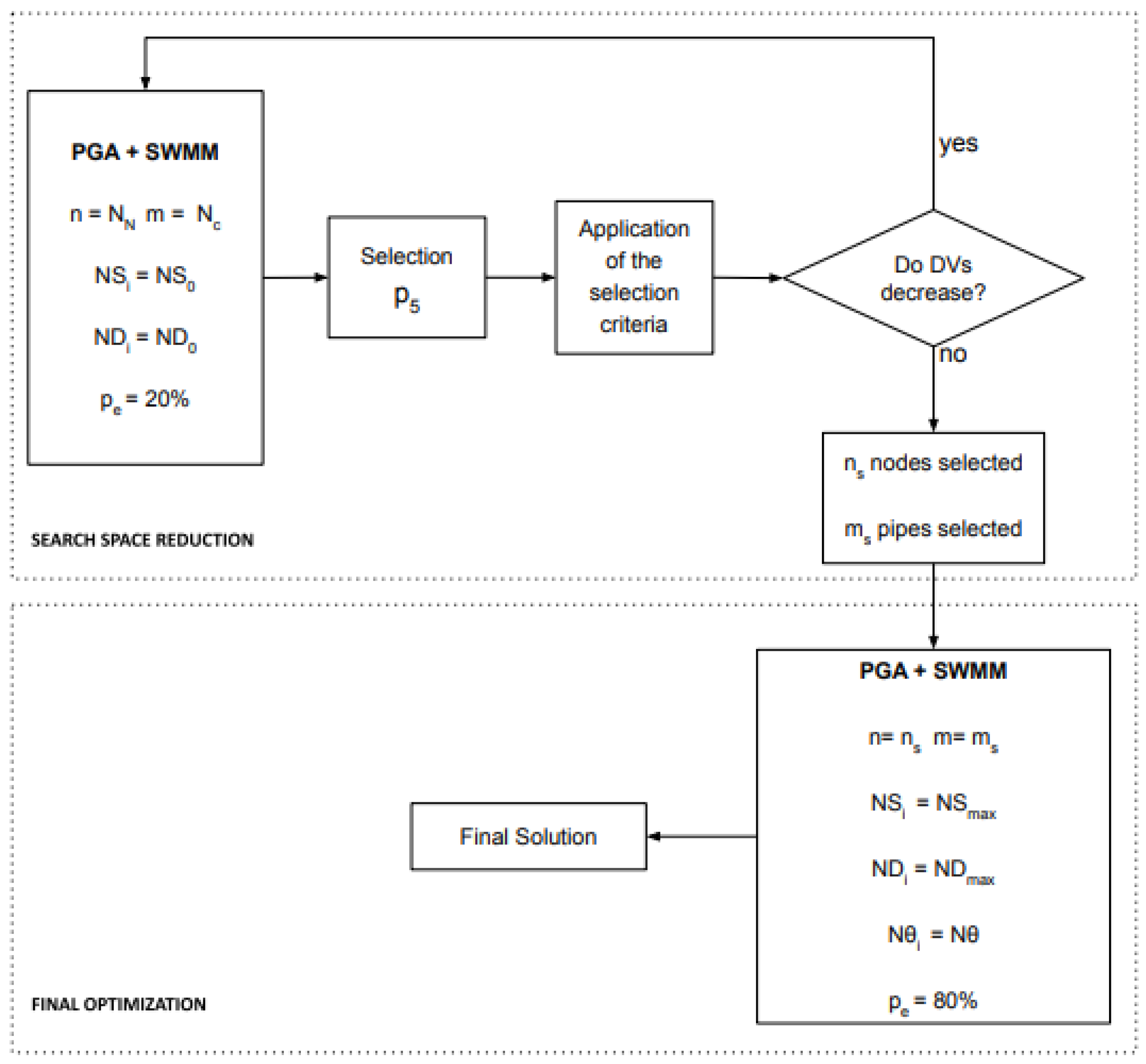
Equations (6)–(9) show the importance of the problem size to define the genetic operators. This is one of the main reasons why the SSR is a useful tool when facing problems from a heuristic approach. In the case of large drainage networks, the large number of DVs becomes an important problem. This high number of DVs demands significant computational effort. The drainage networks consist of branches that serve different sub-catchments, and their runoff flows are added to the network, discharging their waters to a bigger pipe. In other words, the network can be seen as a set of hydraulic sectors (HSs). If these sectors can be identified, a particular analysis of them can be carried out to reduce the number of DVs within the sector and consequently reduce the SS. The optimization process begins by identifying the HSs that composed the network. The optimization model is configured to include the DVs that composed the HS to be optimized. The SSR method is applied to each HS, thereby defining a smaller search region in each HS. Once the SSR process has been carried out for every HS, a new scenario of the network is assembled, where the least prominent regions containing the best solutions have been eliminated. The SSR method is applied to this new scenario to eliminate the least interesting sectors of the new network scenario. Figure 2 illustrates how the application of the sectorized SSR method would work.
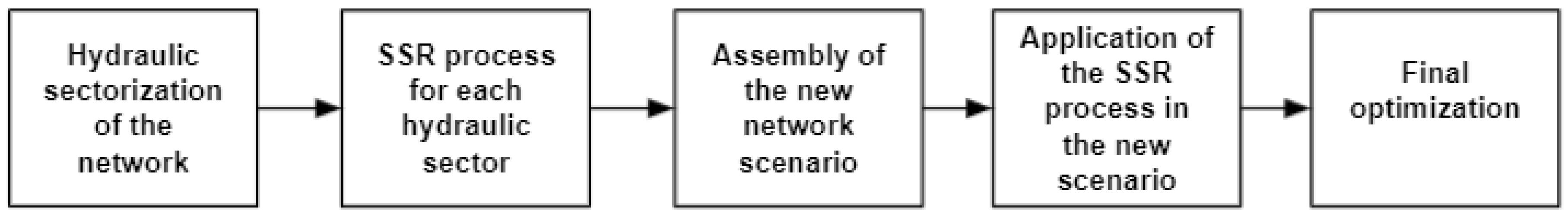
With the reduced problem, a final optimization of the network is carried out to obtain the best solution to the problem posed. The sectorized optimization process is shown in Figure 3.
2.3.2. Reduction in the Number of Options
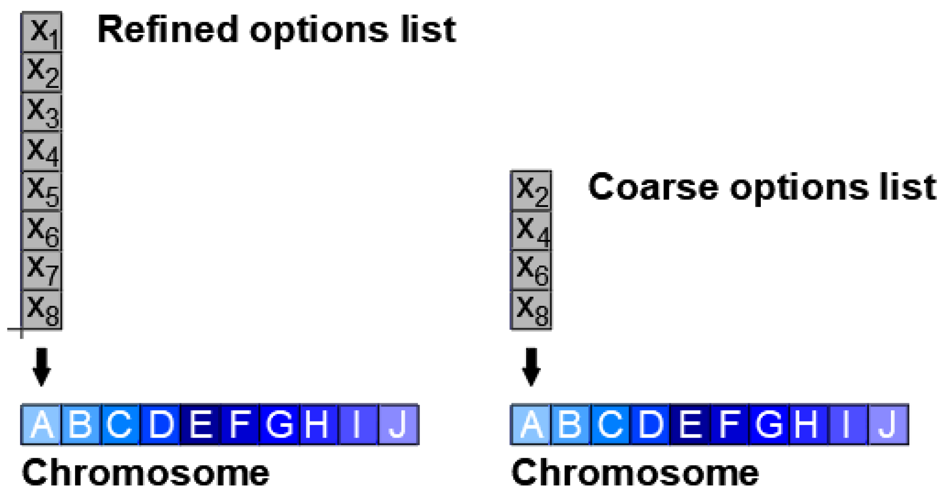
This implies that the quality of a determined solution depends on the time available. If the quality of the solution is not significant for a particular problem, calculation times can be minimized by defining a short list of options. In contrast, a higher quality solution requires a list of options where the separation interval in the discretization is short. It is evident, then, that the value of this separation in the discretization has a preponderant importance in obtaining the result. It can be said that, in an iterative process, such as optimization with genetic algorithms, the quality of the solution will improve if the size of separation used to discretize the DVs is progressively decreased. In this work, two lists of discretization options were determined for each type of DV, one called coarse and the other much refined (Figure 4). These two types of discretization have been determined ensuring that the separation interval allows a good exploration of the SS. Certainly, the coarse options list has a large separation, and it includes separate points, but these points cover the entire SS.
In the case of pipes, as it is a type of discrete variable, the refined options list NDmax corresponded to all pipe diameters available on the market. On the other hand, the coarse options list ND0 was set in such a way that it considered the diameters differentiated and conveniently separated to cover different available ranges that allowed the PGA to make the change of diameter values in the optimization process.
In the case of the DVs that analyzed the nodes where the installation of STs was required, the discretization was performed by dividing the maximum surface into equal intervals. The spacing fixed to discretize the area is called ΔS. Equation (11) was used to calculated ΔS.
where Smax is the maximum area available. In this way, the refined options list N Smax consisted of 40 values, and the coarse options list NS0 consisted of 10 values. The area of each ST is calculated by Equation (12).
where Si is the area of each ST and Xi is the value that the DV takes from the options list.
The volume of each ST is calculated by Equation (13).
where Vi is the volume of the ST and hi is the invert elevation of the ST.
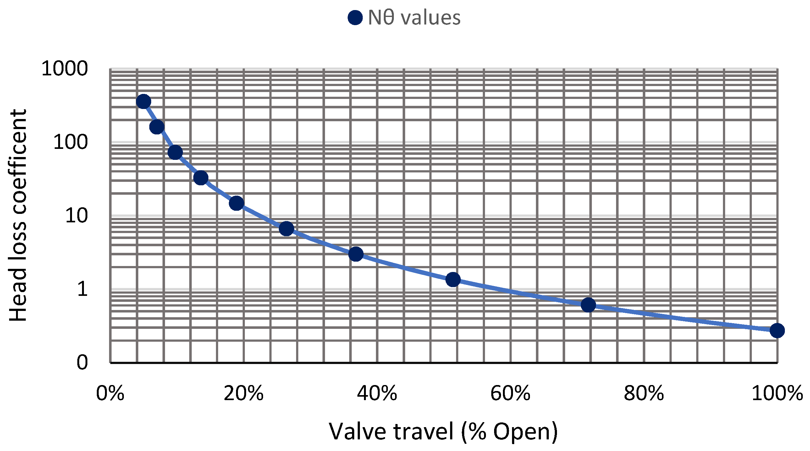
The discretization of the HC opening positions was set according to the valve travel curve presented in Figure 5 and defined in a previous work [18].
To determine the separation interval in the discretization that covers the entire SS, the head loss coefficients (k) are expressed on a logarithmic scale. Consequently, 10 opening positions have been set that allow a good diversity of opening options that composed the options list Nθ for this type of DV. HC is not part of the SSR process, so a coarse options list was not defined for its analysis. Figure 4 shows the Nθ values with the value that each gene represents.
Using a coarse options list obtained a lower quality solution, but the time spent searching for the solution was less. If the chromosome obtained in a low-quality solution is analyzed, it would be observed that it is composed of a chain of genes; each gene represents a value designated to a DV. If a gene has the value 0, it indicates that, in the optimization process, this DV does not require changing its initial condition. If this scenario is repeated in a new calculation, it may be thought that this decision variable does not need to be optimized, and excluding it from the analysis could be considered, reducing the number of DVs and consequently reducing the SS. This procedure is the base of the SS reduction methodology, where sequentially it is sought to eliminate DVs that do not require optimization, keeping the DVs that compose the region that contains the best solutions.
2.3.3. Reduction in the Number of Decision Variables
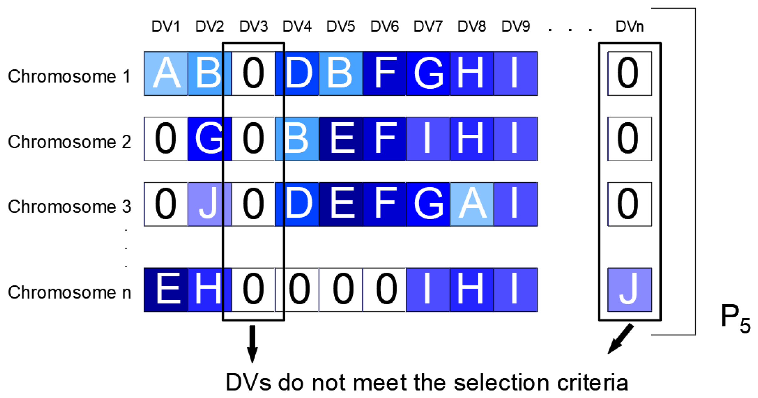
The process of SSR has as a first step a mapping with the optimization model of the entire SS and the decision variables of STs, and pipes are analyzed by the algorithm using a list of options with coarse discretization. The use of a coarse options list allows the identification of the DVs that may be included in the most promising region of the algorithm’s exploration space. For this, a certain number of evaluations Nit is established, and from the results obtained the fifth percentile (P5) of the solutions is selected. In the selected P5, each chromosome is analyzed, quantifying how many genes different from 0, called valid genes, have been obtained for each DV. If a DV does not have at least 20% valid genes, it is assumed that this DV is not part of the promising region of the SS, and it is eliminated from the new SS. If, on the contrary, a DV presents a high repeatability of valid genes, it is considered a candidate to be contained in the most promising search region. The percentage of 20% is then established as the criterion for the selection of variables to be considered in the SS. Figure 6 shows an example of how the selection criteria work in the SSR.
The process is repeated in the new defined region, eliminating the DVs that do not meet the selection criteria. In each iteration of the process, the convergence of the results towards certain DVs whose repeatability in the sampling increases, each time defining the region with the best solutions. The process ends when all variables meet the selection criteria, and the SS cannot be further reduced. In the SSR process, Pe is set at 20%. This percentage is used to find solutions without demanding a lot of calculation time. The reason why a Pe of 20% is used is because, in this process, it is not a goal to find the final solution, but to eliminate DVs to reduce the SS.
2.4. Final Optimization
Once the final search region is defined, the final optimization is performed in this new scenario. The refined options list for pipes, NDmax, and the refined options list for STs, NSmax, are used in this optimization. At this stage, the HCs are also included in the optimization model, so the options list Nθ is also used. With the optimization model configured in this way, a much finer exploration of the reduced space is intended, since it is assumed that the global optimum is found in this region. With this objective in addition, a much more demanding stopping criterion is used with a Pe equal to 80%. It should also be noted that the value of Xmax in Equation (8) increases because the refined discretization is used. With the Gmax defined in this way, the model is expected to demand a higher computational effort. However, with the objective of finding the closest solution to the optimal solution, this effort is justified. The proposed optimization process is summarized in Figure 7.
2.5. Application of the Model
2.5.1. E-Chico Network
To apply the methodology, the E-Chico network located in the city of Bogotá, Colombia was selected. This network has 35 hydrological sub-basins that occupy an area of 51 hectares, 35 conduits, and 35 connection nodes. All pipes are circular, and their diameters range from 300 mm to 1400 mm. The network is approximately 5000 m long. This network has the particularity of being in the foothills of the Andes Mountain Range, which makes it have steep slopes with a difference in level of 39 m between the lowest and highest point of the network; these characteristics make the operation of this network totally dependent on gravity. The hydraulic model of the network was made by Saldarriaga et al. in a previous work [30]. In an actual state and for a design storm with a return period of 10 years, the urban basin generates a runoff of 20,123 m3, and has a flood volume of 3834 m3, which represents 19.07% of the runoff volume and concentrates in 11 nodes of the network.
For the analysis of the network, a design storm was used based on an intensity-duration-frequency curve, previously defined by Ngamalieu-Nengoue et al. [17]. This design storm was calculated using the alternate block method with 5-min intervals from an IDF curve for a return period of 10 years and a calculated duration of 55 min. The maximum intensity was limited to 118 mm/h, corresponding to a duration of 10 min to avoid very high intensities.
According to its configuration, two hydraulic sectors, HS-1 and HS-2, could be identified in the network (Figure 8). HS-1 composed the upper part of the network with 17 pipes and 17 nodes, while HS-2 composed the lower part of the network with 14 pipes and 14 nodes. Although smaller sectors might be identified, the number of DVs of these branches was too small to be interesting enough to analyze them separately. Therefore, separating the network into two sectors was considered a more advantageous option. The nodes and pipes excluded from both sectors were added to the optimization process in the assembly of the new scenario that was generated after reducing the SSR process of the SHs.
The PGA parameters that were applied to the optimization model to start the SSR process are those shown in Table 1. Once the SS was reduced, the final optimization was applied to the resulting region. The parameters used in this stage are those shown in Table 1. To carry out the optimization, Nit = 250 was defined for each proposed iteration. With this value, it was expected to have enough iterations to achieve convergence towards a satisfactory solution.
For the calculation of the objective function, the coefficients of the cost functions defined in Equations (1)–(4) were determined. These coefficients were defined for the case study according to the costs of the Colombian economy. Table 2 shows the coefficients for the infrastructure cost functions. Equation (14) shows the coefficients for calculating the cost of flood damage.
2.5.2. Ayurá Network
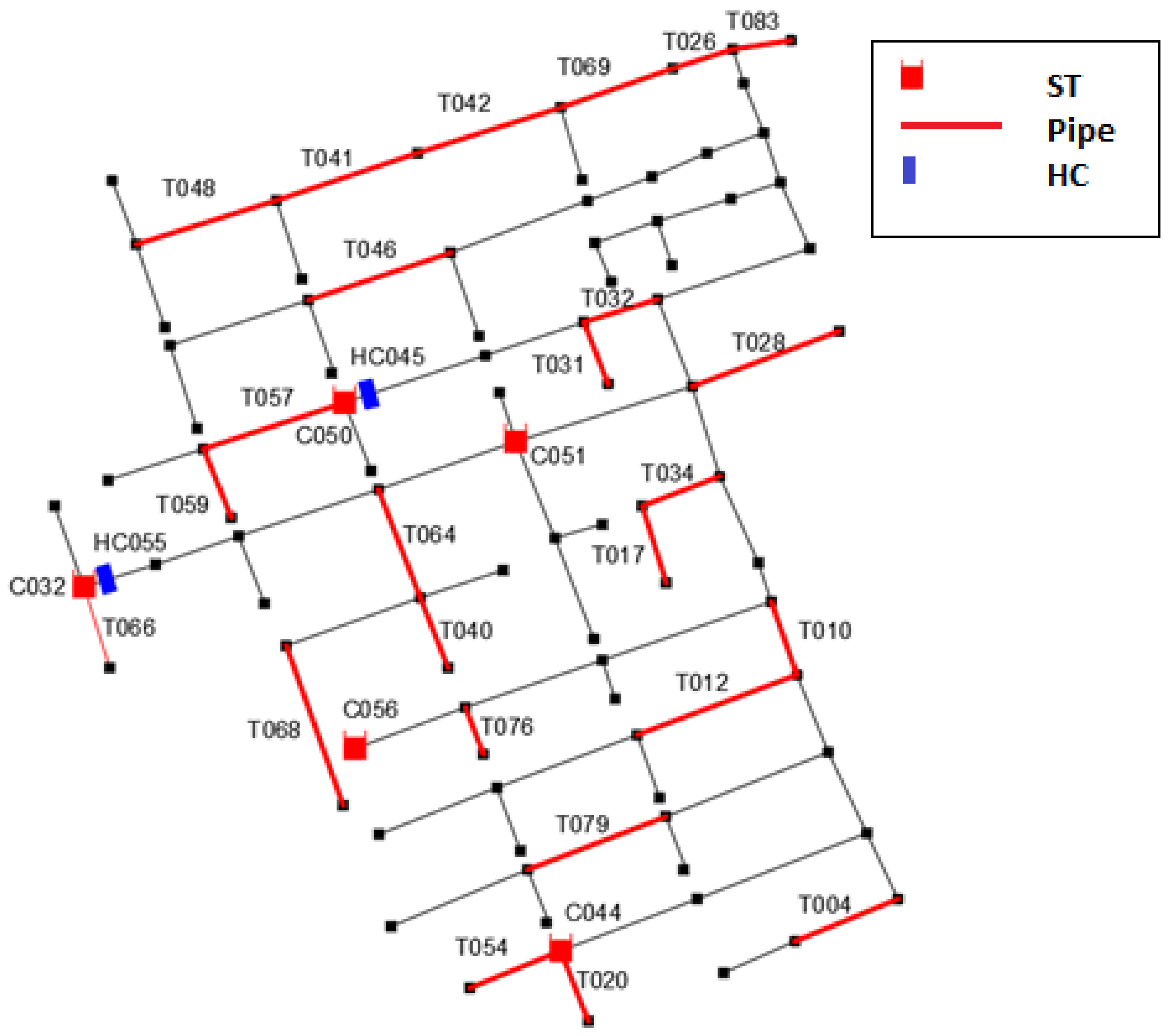
The method was applied to a second network of larger dimensions. This second network corresponded to a neighborhood in the city of Medellín, Colombia called Ayurá. The network crosses the city from south to north, and covers an area of 22.5 ha divided into 96 sub-basins. The network is composed of 86 nodes and 86 circular ducts, with a diameter ranging from 200 mm to 1050 mm. The difference in levels between the highest point of the network and the lowest is 14.61 m. These characteristics make the operation of the network entirely dependent on gravity. The average slope of the pipes that compose the network has a value of 1.81%.
For the analysis of the network, a design storm calculated by the method of alternate blocks was used. The total runoff from the network in the scenario studied is 13,970 m3. The flooding in different nodes of the network has a total value of 4012 m3, which represents 28.72% of the total runoff.
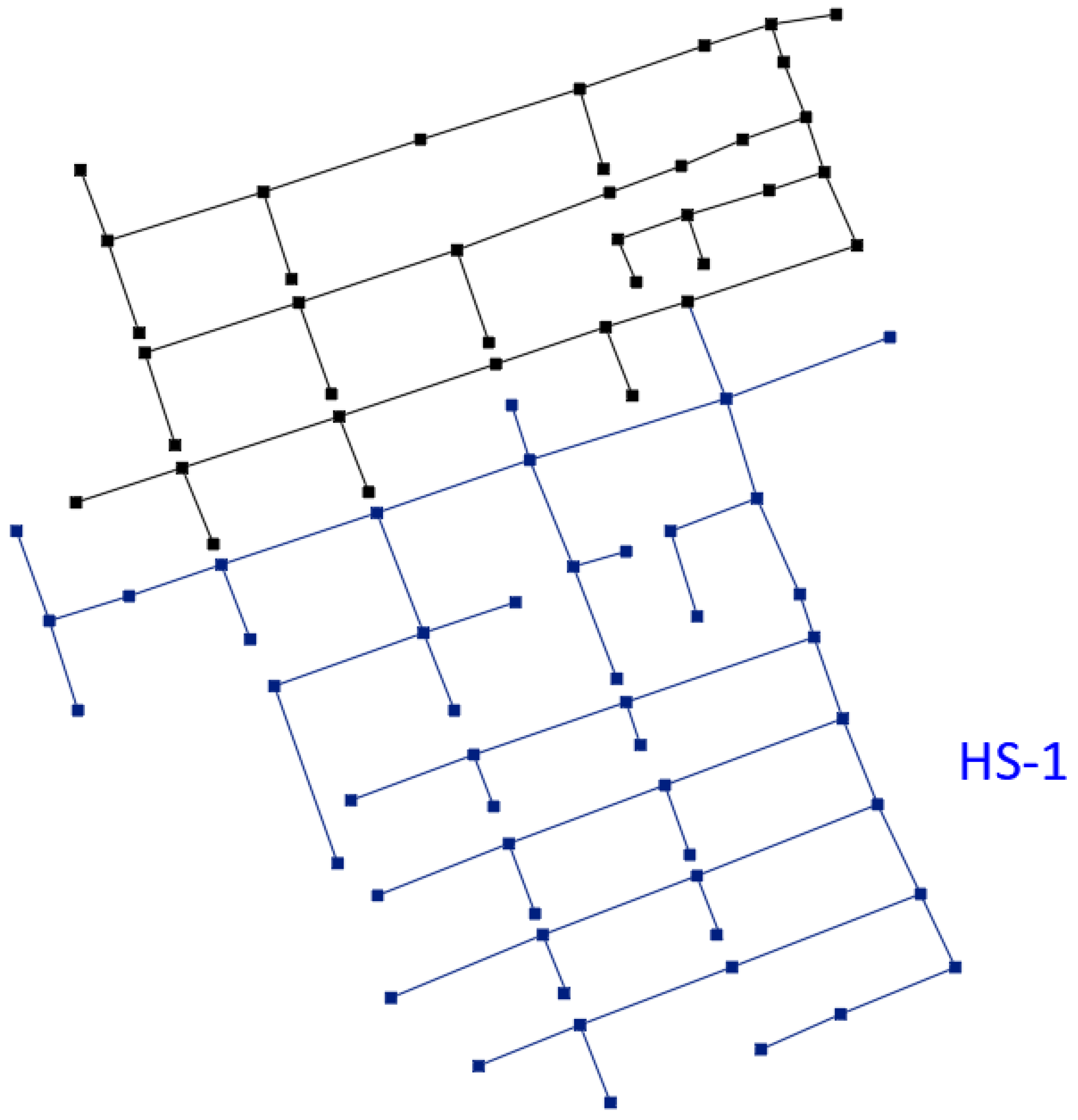
The network topology does not allow for differentiation of specific HSs. The network is composed of different branches that are connected to a principal line. To face the optimization problem, it was decided to divide the network into two sectors (Figure 9). A sector called HS-1 considered the upper part of the network with 49 nodes and 49 pipes where the SSR methodology was applied. Once the optimal region of HS-1 was defined, a new scenario was formed in which the SSR process was applied again, defining a final reduced region. Lastly, a final optimization was performed in the determined region to find the best solution to the optimization problem. Table 3 shows the parameters initially used by the PGA for each scenario proposed. To divide the network into two sectors, it was considered that the network was composed of 258 DVs corresponding to pipes, STs, and HCs, so analyzing it completely would increase the SS that the PGA must explore. For this reason, optimizing the network by sectors would mean reducing the calculation times. On the other hand, analyzing the network in sectors allows reducing the DVs considered in the optimization process, which would determine a stop criterion defined by Equation (8) to decrease considerably. Specifically, when analyzing HS-1 in the first part, the stopping criterion was reduced by 24% when applying the SSR methodology compared to if it were applied throughout the network.
3. Results
3.1. E-Chico Network
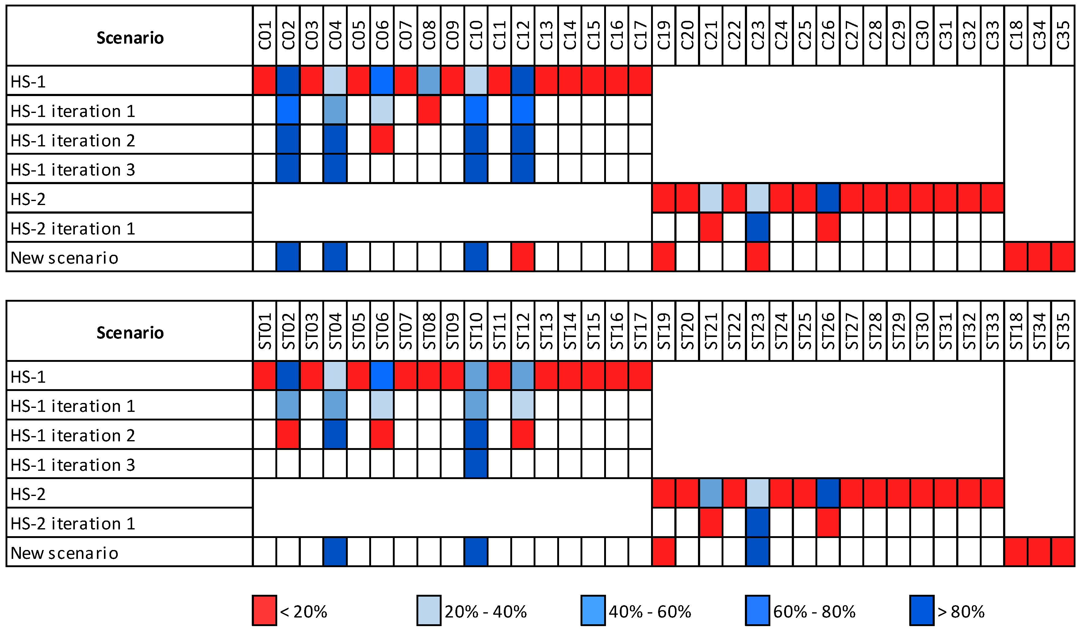
Figure 10 summarizes the SSR process in the E-Chicó network. In the first step, HS-1 and HS-2 were processed separately. Once the number of variables was reduced, a new scenario was set up with the remaining DV from HS-1, HS-2, and the elements not included in any HS (conduits C18, C34, and C35, and the corresponding tanks ST18, ST34, and ST35). The results showed that certain DVs had a higher repeatability. By applying the selection criteria, the areas of the SS that were less interesting to explore were eliminated, thus defining a new SS. While the SS was reduced, the repeatability increased in the most promising DVs to be considered in the final analysis region. With the SS reduced in the HSs, the new search scenario was assembled that included the nodes and pipes obtained in the previous process and elements of the network that had not been analyzed. To perform the final optimization, the DVs of the HCs must be added to this region.
Table 4 shows the reduction of the SS in each iteration of the optimization model; the SS was reduced from a magnitude of 140, which would be obtained when optimizing the network without any type of SSR strategy, to a magnitude of 12 once the proposed method was applied. In the final scenario, the DVs corresponding to the HCs were added.
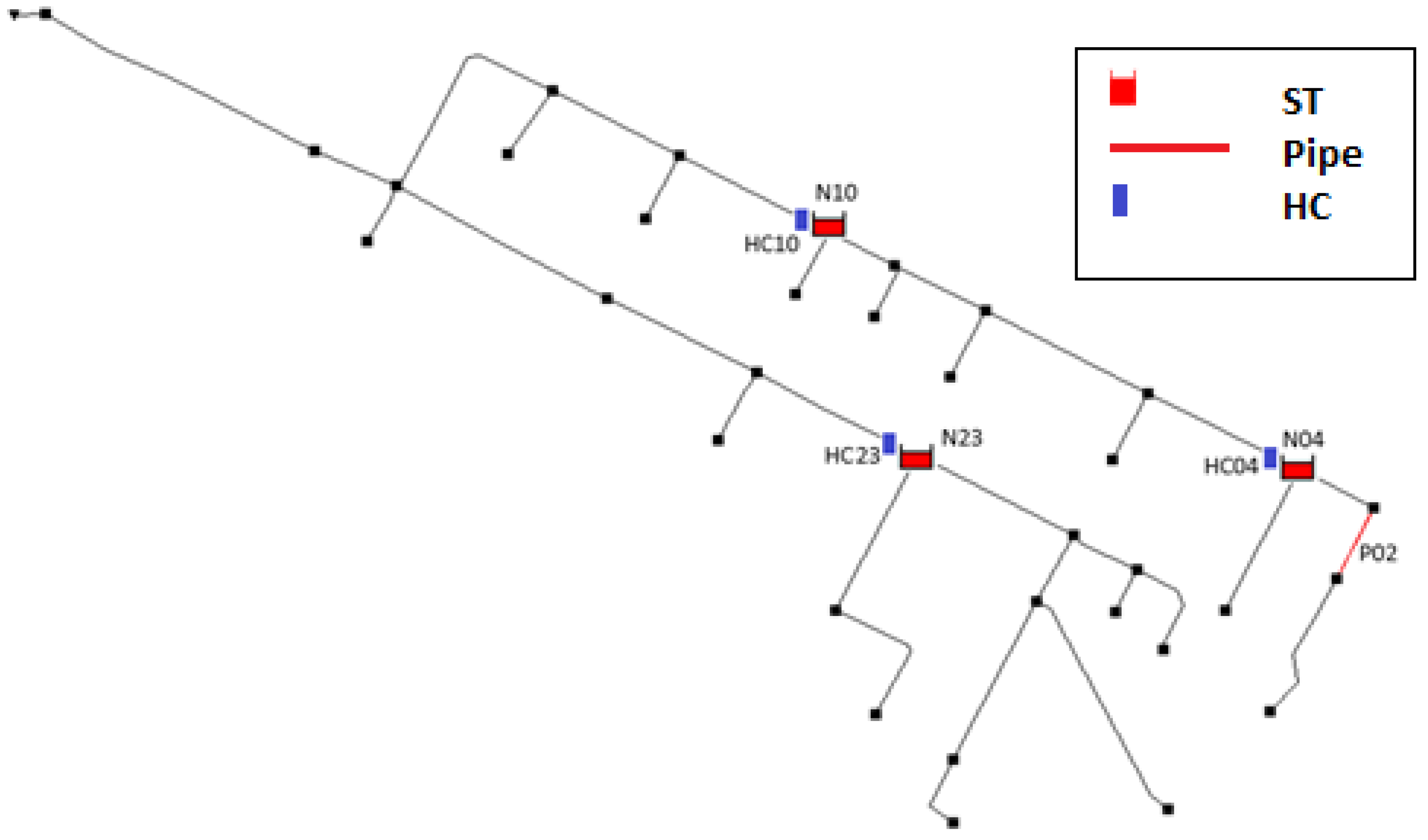
The final solution required the renewal of a pipe (C02) that increased its diameter from 0.4 m to 0.5 m. The installation of STs was in nodes N04, N10, and N23 with volumes of 1462 m3, 2300 m3, and 1958 m3, respectively. The installation of HCs in the pipes C04, C10, and C23 had k values of 72.55, 14.73, and 14.73, respectively. Figure 11 illustrates the elements to be installed in the network. The costs of the final solution found by the optimization model are shown in Table 4. With these actions, we had the necessary infrastructure costs to optimize the network as follows: cost of pipes = 6583.81 €, cost of STs = 179,757.70 €, and cost of HCs = 7671.78 €. The cost of flood damage was 5700.66 €. Thus, the objective function took the value of 199,713.95 €. This value contrasted with the cost obtained when applying a standard GA optimization without SSR. In the latter case, the optimal value found after 250 runs of the algorithm was 251,711.79 € (26% more expensive).
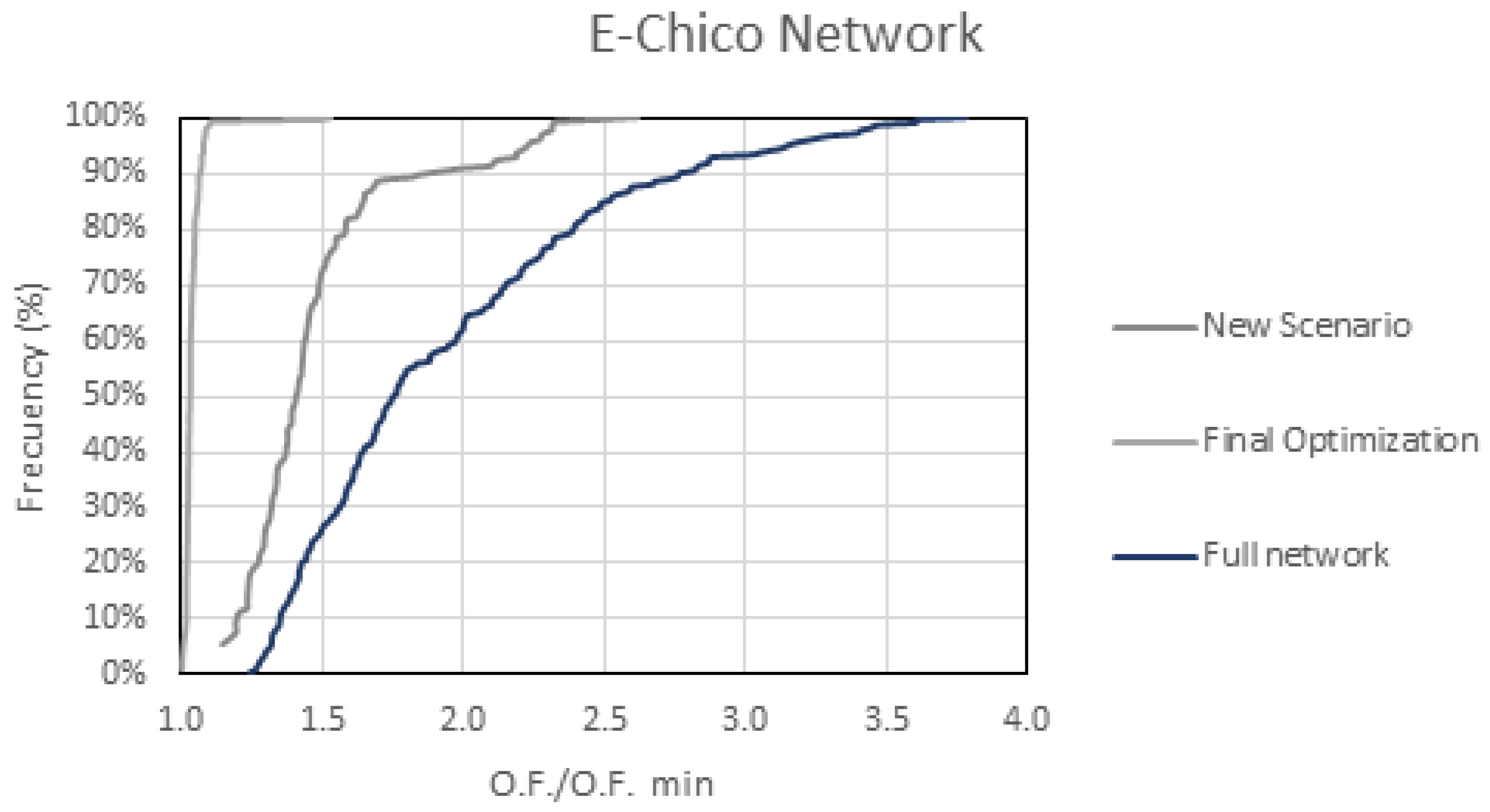
Figure 12 shows the comparison between the different scenarios when reducing the SS and optimizing the E-Chico network without the application of a previous SSR process. The value of the minimum objective function in each simulation carried out is represented on the x-axis, and the accumulated frequency with which this value appears in the Nsim is on the y-axis. This figure is used to see the degree of dispersion of the results obtained in the simulation. The optimization process is more efficient if the curve has a greater slope. The final optimization curve shows the advantages of applying the SSR method in a first stage. This figure also shows that the dispersion of the results obtained for the objective function was reduced as the number of decision variables decreased.
3.2. Ayurá Network
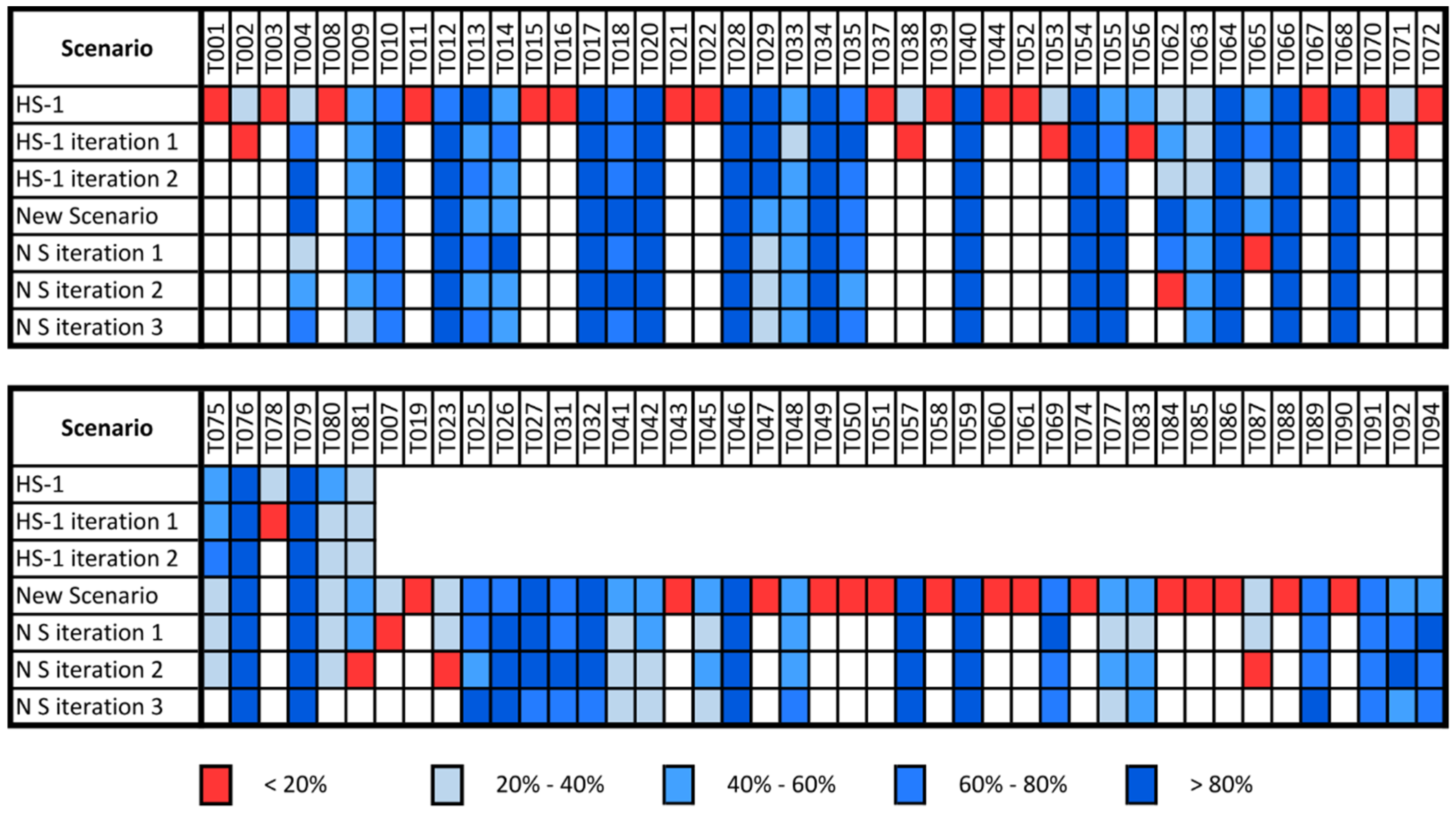
Figure 13 and Figure 14 show the application of SSR to the tanks and conduits of the Ayurá network, respectively. As it can be easily observed, the search region was noticeably reduced in only two iterations in the HS-1, mainly in the case of tanks (Figure 13). After reducing the number of DVs in HS-1, a new scenario was defined. The SSR process was then applied to this new scenario. Finally, the DVs corresponding to the HCs were added to this new scenario for the final optimization of the network.
Table 5 summarizes the search space for the entire network and for each scenario in the Ayurá network SSR process.
The final solution required the renovation of 25 pipes, the installation of five STs, and the inclusion of two elements of hydraulic controls at the outlet of the STs. Table 6 shows the diameters of the network in an initial state and the optimized diameters of the pipes to be installed. Table 7 shows the characteristics of the STs and HCs that must be installed according to the results obtained. Figure 15 illustrates the elements to be installed in the network. Specifically, the final solution has an objective function of 328,049.63 €. The cost of the renewal of the pipes had a value of 112,297.59 €, the cost of the installation of STs had a value of 201,454.17 €, and the cost of the installation of HCs had a value of 2768.62 €. The cost of the damage caused by the floods had a value of 1529.25 €.
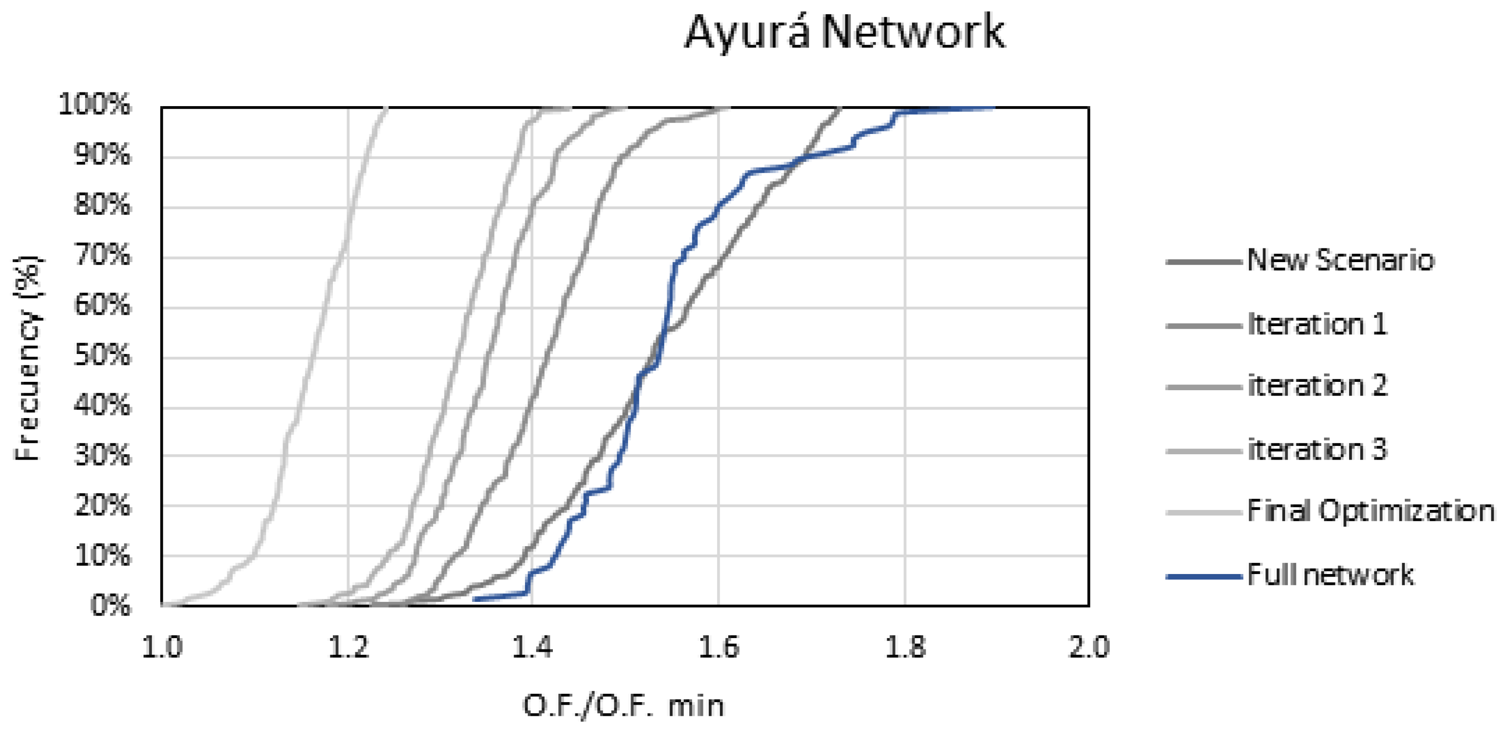
Figure 16 compares the results when optimizing the full network without applying the SSR method (blue line) and the different iterations carried out until optimization is achieved with the proposed method (set of gray-scaled lines). Both methodologies were repeated 250 times. The figure shows on the x-axis the relationship of the objective function of each result with the minimum objective function found. The y-axis represents the accumulated frequency. The values represented correspond to the established Nsim (250 in this case). As can be seen, the optimization process improved remarkably by applying the SSR method iteratively. Finally, the curve corresponding to the final optimization was obtained with a greater slope of the curve, which indicated that, in this scenario, the dispersion of solutions was lower. To better appreciate how the dispersion of the results decreased with the proposed methodology, the comparison of these results with the optimization without previously applying the SSR process is shown in Figure 17.
4. Discussion
The methodology presented in this work considers different types of decision variables: pipes, storm tanks, and hydraulic controls. Consequently, there is a large search space. To solve this problem, a process is presented to reduce this search space. The analysis of this discretization has been made considering that the sampling points cover the entire search space and that the process is applicable to any type of network. However, a previous detailed study showed that the characteristics of the network, maximum and minimum diameters installed, and available flood area can shorten the size of the options list for each decision variable by reducing the initial search space and decreasing the definition time of the final search region. This is one of the fields that can be explored in future work. On the other hand, to discretize the continuous decision variables, two spacing values are adopted that generate two lists of options, one called rough and the other called refined. One limitation of the presented method is that the spacing has been established according to the criteria of the authors, and although it is true that covering the search space in the best way has been tried, future works should consider the establishment of this spacing by analyzing the influence of the algorithm parameters.
Another aspect to discuss in this work is the different percentages used as the probability of success when establishing the stopping criteria. The use of a low probability of success (Pe = 20%) in the SSR process aims to eliminate DVs. This elimination assumes that if, with a loose value of Pe, the repeatability of a DV is low, it is assumed that this DV will not be part of the region of best solutions. In the figures (repeatability figures), it can be observed how the repeatability in the most promising DVs increases as the SS decreases, while the DVs that present a low repeatability disappear in subsequent iterations. These facts emphasize the value of the presented method to identify the region with the best solutions within the SS. However, the use of more demanding values of Pe as the search region is reduced is presented as an interesting option to improve the efficiency of the process. This is undoubtedly an aspect that should be analyzed in depth in future work. In this work, the concept of reducing the search space by hydraulic sectors has also been introduced. This way of applying the search space reduction method is presented as an interesting option that allows the optimization model to work in parallel, able to define the search region faster than when analyzing the entire network, although it is true, in the optimization of the Ayurá network, that the hydraulic sectors are not clearly differentiated. Dividing the network into two parts allows us to have a manageable number of DVs by optimizing the network. Applying the SSR process at the top of the network at first and incorporating the selected DVs at the bottom part of the network reduces significantly the computational effort required. In the case of the E-Chico network, two sectors, called HS-1 and HS-2, are clearly differentiated. In this network, it can be seen how the repeatability increases in each iteration until presenting a repeatability of 100% in the selected DVs. Additionally, Figure 17 compares the dispersion of the solutions of the results when applying the proposed methodology in the studied networks and when optimizing the networks without applying any SSR process. In Figure 17, it is clearly observed that, when optimizing the complete network, the dispersion of the results is greater, having values of the objective function up to 3.7 times greater than the minimum value, while, when applying the proposed methodology, the dispersion of the results decreases significantly. The curve obtained in the final optimization has a greater slope, and the variation of the results found is reduced by about 1.50 times. In the Ayurá network (Figure 16), there are similar results; the optimized network without any SSR process has a greater dispersion of results, having objective function values of up to 1.90 times greater than the minimum value found. This shows us that optimizing networks with a large number of DVs increases the dispersion of the solutions. Therefore, applying the SSR process not only reduces calculation time, but also improves efficiency in optimization. These particularities were already observed by Ngamalieu et al. [16] in a previous work.
On the other hand, the results show that, when optimizing the network by sectors, the values of N and Gmax decrease; this is because their value depends on the number of DVs analyzed by the PGA. Therefore, the calculation times and the computational effort are going to be much less than when optimizing the entire network. This shows us that the methodology can be indicated to optimize large networks. In another order of things, the results obtained from Nsim in Table 5 show that the number of iterations that each simulation requires to find the solution decreases in each application of the SSR process. These results are presented in the two networks studied, so it can be said that the methodology presented improves the efficiency of the optimization. For the final optimization, using a refined optimization and a more demanding Pe, the number of simulations increases. Considering that the objective is to find the best solution in a reduced SS, this increase is fully justified. In the Ayurá network (Table 6), it is observed that, in each iteration, the iterations decrease, having a Nsim = 3127 in the new scenario until Nsim = 967 in the third iteration. Optimizing the network by sectors has clear benefits. The decrease in the objective function is clearly observed in Figure 17 when compared to the optimization of the network without applying the SSR process. The figure shows that the largest dispersion of the optimized network without an SSR process is found in the first quartile. On the other hand, it can be observed that the best result of the optimized network without applying the SSR process has a higher value than the worst value of the final optimization of the proposed methodology. In the Ayurá network (Figure 17), there are similar results, and it is observed that the highest number of results in the final optimization is in the last quartile, which reflects the suitability of the methodology.
The final optimization shows the suitability of applying the optimization methodology with the installation of STs, renewal of pipes, and installation of HCs. The use of a more demanding stopping criterion can guarantee us that the search for the best solutions in the final search region is carried out intensively. For these reasons, this form of optimization should be investigated in greater depth, as it could provide interesting results in terms of reducing calculation times in the face of this type of problem.
Lastly, technological advancement and limited resources have motivated the development of new research strategies to optimize time and economic resources. Algorithms have been consolidated as a valid tool to facilitate this task. Their use in different fields of research has been popularized in recent years. In problems of water resources, GAs have had a relevant use [32,39,40]. GAs have been applied in subjects such as water distribution systems and closely related applications, urban drainage and sewer system applications, water supply and wastewater treatment applications, applications in hydrologic and fluvial modeling, groundwater system applications, groundwater remediation, groundwater monitoring, and evolutionary computation in hydrologic parameter identification. The proposed SSR methodology considers the iterative elimination of DVs from a problem, and can be applied to other types of problems with a similar approach. This may be a contribution of the present work for future developments in the field of optimization through evolutionary strategies.
5. Conclusions
The increase in flood events in different cities of the world makes it necessary to develop methodologies to face them, considering the improvement of the systems with the lowest possible cost. The use of heuristic approaches is a good alternative to solve this type of problem. The methodology based on the optimization of the network considering the replacement of pipes, installation of storm tanks, and inclusion of hydraulic controls has proven to be a valid alternative to solve these types of problems. To improve the efficiency of the optimization model, this work focuses on presenting a methodology for reducing the search space for solutions to improve the working efficiency of the optimization model. The application of this methodology significantly reduces the number of total iterations when compared to the initial scenario, that is, if it will perform the optimization with all of the decision variables.
In the E-Chico network in particular, the SS is reduced from a magnitude of 140 to a magnitude of 12, while, in the Ayurá network, much larger than E-Chico, the SS is reduced from a magnitude of 344 to one of 82. If it is considered that the size of the SS is measured in a logarithmic scale, it can be seen that a significant reduction has been made. These results show that the search space reduction method is valid and advantageous to apply in optimization problems with drainage networks. For the Ayurá network, the improvement of the results can be observed more greatly when applying the proposed method than in the complete network without any previous reduction of the SS. On the other hand, if the results obtained from the E-Chico network are compared with the results obtained in a previous study [18], it can be seen that the objective function of the problem has been reduced, including the cost of flood damage. Therefore, it can be concluded that by using the method of SSR based on the use of a coarse discretization of the decision variables and a lax stop criterion in the first stage, as well as a refined discretization and a demanding stop criterion in the second stage, the efficiency of the optimization model is improved. The two cases presented have been applied to drainage networks located in Colombia, and thus were expressed in terms of the local Colombian economy, the investment costs in infrastructure, and the costs associated with flood damage. In this way, formulating cost functions in monetary units is very useful for decision makers in the development of a rehabilitation project.
New trends are focused on source control by means of LID techniques. Future works must address the possibility of combining the strategy presented in this work with another focused on the reduction of runoff using components such as green roofs, pervious pavement, or infiltration structures.
Finally, the results obtained show a good solution for a previously defined rain. Different results will be obtained for other design storms. Therefore, there is no single solution to the problem, and the initial approaches to the problem will be made in accordance with design criteria and local regulations.
Author Contributions
All authors contributed extensively to the work presented in this paper. Conceptualization, L.B.-J., P.L.I.-R. and F.J.M.-S.; data curation, L.B.-J. and F.J.M.-S.; formal analysis, L.B.-J., P.L.I.-R. and F.J.M.-S.; funding acquisition, D.M.-M.; investigation, L.B.-J., P.L.I.-R., F.J.M.-S. and D.M.-M.; methodology L.B.-J., P.L.I.-R., F.J.M.-S. and D.M.-M.; project administration P.L.I.-R. and F.J.M.-S.; resources, L.B.-J., P.L.I.-R., F.J.M.-S. and D.M.-M.; software, L.B.-J., P.L.I.-R. and F.J.M.-S.; supervision, P.L.I.-R., F.J.M.-S. and D.M.-M.; validation, L.B.-J., P.L.I.-R., F.J.M.-S. and D.M.-M.; visualization, L.B.-J., P.L.I.-R., F.J.M.-S. and D.M.-M.; writing—original draft, L.B.-J., P.L.I.-R., F.J.M.-S. and D.M.-M.; writing—review and editing, L.B.-J., P.L.I.-R., F.J.M.-S. and D.M.-M. All authors have read and agreed to the published version of the manuscript.
Funding
This research was funded by the Program Fondecyt Regular, grant number 1180660.
Institutional Review Board Statement
Not applicable.
Informed Consent Statement
Not applicable.
Data Availability Statement
Not applicable.
Acknowledgments
This work was supported by the Program Fondecyt Regular (Project No. 1210410 and Project No. 1180660) of the Agencia Nacional de Investigación y Desarrollo (ANID), Chile.
Conflicts of Interest
The authors declare no conflict of interest.
Abbreviations
The following abbreviations are used in this manuscript:
| GA | Genetic Algorithm |
| DV | Decision Variable |
| HC | Hydraulic Control |
| HS | Hydraulic Sector |
| LID | Low Impact Development |
| OF | Objective Function |
| PGA | Pseudo Genetic Algorithm |
| SS | Search Space |
| SSR | Search Space Reduction |
| ST | Storm Tank |
| SWMM | Storm Water Management Model |
Notations
The following symbols are used in this paper:
| CC(Di) | cost of the installation of the hydraulic control |
| CD(Di) | cost of the renovation of pipes |
| Cmax | maximus cost per square meter that cause a flood |
| Cmin | minimum cost established for the storm tank |
| CV(Vi) | cost of installation of the storm tank |
| Cvar | constant in the cost function of storm tanks |
| Cy(yi) | damage costs caused by the flood |
| Di | diameter of pipe (m) |
| Gmax | stop criterion |
| hi | invert elevation of storm tank |
| k | head loss coefficient in valves |
| Li | pipe length (m) |
| m | pipes |
| mi | pipes considered in a defined scenario |
| ms | pipe selected to be replaced |
| N | population size |
| NS | options list for storm tanks |
| NS0 | coarse options list for storm tanks |
| NSmax | refined options list for storm tanks |
| n | nodes |
| ni | nodes considered in a defined scenario |
| NC | number of pipes in the network |
| ND | options list for pipes |
| ND0 | coarse options list for pipes |
| NDmax | refined options list for pipes |
| NDV | number of decision variables |
| Nit | number of evaluations |
| Nsim | number of simulations in each evaluation |
| NN | number of nodes in the network |
| ns | number of nodes selected to install storm tanks |
| Nθ | options list for hydraulic controls |
| P5 | fifth percentile |
| Pe | success probability |
| pi | pipes considered to install hydraulic controls in a defined scenario |
| Pmut | mutation probability |
| PO | occurrence probability |
| ps | pipes selected to install hydraulic controls |
| r | adjustment coefficient of the cost of flood. |
| Si | area of storm tank (m2) |
| Smax | maximum area available (m2) |
| Vi | storage volume (m3) |
| Xi | value of decision variable taken from the options list for storm tanks |
| Xmax | maximum number of discretization options of the decision variables |
| yi | water level of the node (m) |
| ymax | maximus flood level (m3) |
| α | adjustment coefficient of the cost of pipes |
| β | adjustment coefficient of the cost of pipes |
| γ | adjustment coefficient of the cost of hydraulic control |
| ΔS | spacing interval in the discretization of area of storm tank |
| λ | adjustment coefficient of the cost of flood |
| δ | constant for the calculation of the mutation probability |
| μ | adjustment coefficient of the cost of hydraulic control |
| ω | exponent in the cost function of storm tanks |
| ϕ | constant for calculation of population |
References
- Kaykhosravi, S.; Khan, U.T.; Jadidi, M.A. The effect of climate change and urbanization on the demand for low impact development for three Canadian cities. Water 2020, 12, 1280. [Google Scholar] [CrossRef]
- Ma, B.; Wu, Z.; Wang, H.; Guo, Y. Study on the Classification of Urban Waterlogging Rainstorms and Rainfall Thresholds in Cities Lacking Actual Data. Water 2020, 12, 3328. [Google Scholar] [CrossRef]
- Zhuang, Q.; Liu, S.; Zhou, Z. Spatial Heterogeneity Analysis of Short-Duration Extreme Rainfall Events in Megacities in China. Water 2020, 12, 3364. [Google Scholar] [CrossRef]
- Agarwal, S.; Kumar, S. Applicability of SWMM for semi urban catchment flood modeling using extreme rainfall events. Int. J. Recent Technol. Eng. 2020, 8, 245–251. [Google Scholar]
- Ciupa, T.; Suligowski, R. Impact of the City on the Rapid Increase in the Runoff and Transport of Suspended and Dissolved Solids During Rainfall—The Example of the Silnica River (Kielce, Poland). Water 2020, 12, 2693. [Google Scholar] [CrossRef]
- Jha, M.; Afreen, S. Flooding Urban Landscapes: Analysis Using Combined Hydrodynamic and Hydrologic Modeling Approaches. Water 2020, 12, 1986. [Google Scholar] [CrossRef]
- Leal, M.; Boavida-Portugal, I.; Fragoso, M.; Ramos, C. How much does an extreme rainfall event cost? Material damage and relationships between insurance, rainfall, land cover and urban flooding. Hydrol. Sci. J. 2019, 64, 673–689. [Google Scholar] [CrossRef]
- O’Donnell, E.C.; Thorne, C.R. Drivers of future urban flood risk, Philosophical Transactions of the Royal Society A: Mathematical. Phys. Eng. Sci. 2020, 378, 2168. [Google Scholar]
- Mora-Melià, D.; López-Aburto, C.S.; Ballesteros-Pérez, P.; Muñoz-Velasco, P. Viability of Green Roofs as a Flood Mitigation Element in the Central Region of Chile. Sustainability 2018, 10, 1130. [Google Scholar] [CrossRef] [Green Version]
- Iglesias-Rey, P.L.; Martínez-Solano, F.J.; Saldarriaga, J.G.; Navarro-Planas, V.R. Pseudo-genetic Model Optimization for Rehabilitation of Urban Storm-water Drainage Networks. Procedia Eng. 2017, 186, 617–625. [Google Scholar] [CrossRef]
- Carter, T.; Jackson, C.R. Vegetated roofs for stormwater management at multiple spatial scales. Landsc. Urban Plan. 2007, 80, 84–94. [Google Scholar] [CrossRef]
- Mentens, J.; Raes, D.; Hermy, M. Green roofs as a tool for solving the rainwater runoff problem in the urbanized 21st century? Landsc. Urban Plan. 2006, 77, 217–226. [Google Scholar] [CrossRef]
- Andrés-Doménech, I.; Montanari, A.; Marco, J.B. Efficiency of storm detention tanks for urban drainage systems under climate variability. J. Water Resour. Plan. Manag. 2012, 138, 36–46. [Google Scholar] [CrossRef]
- Cunha, M.C.; Zeferino, J.A.; Simões, N.E.; Saldarriaga, J.G. Optimal location and sizing of storage units in a drainage system. Environ. Model. Softw. 2016, 83, 155–166. [Google Scholar] [CrossRef] [Green Version]
- Wang, M.; Sun, Y.; Sweetapple, C. Optimization of storage tank locations in an urban stormwater drainage system using a two-stage approach. J. Environ. Manag. 2017, 204, 31–38. [Google Scholar] [CrossRef] [PubMed]
- Ngamalieu-Nengoue, U.A.; Iglesias-Rey, P.L.; Martínez-Solano, F.J.; Mora-Meliá, D.; Valderrama, J.G.S. Urban drainage network rehabilitation considering storm tank installation and pipe substitution. Water 2019, 11, 515. [Google Scholar] [CrossRef] [Green Version]
- Ngamalieu-Nengoue, U.A.; Martínez-Solano, F.J.; Iglesias-Rey, P.L.; Mora-Meliá, D. Multi-objective optimization for urban drainage or sewer networks rehabilitation through pipes substitution and storage tanks installation. Water 2019, 11, 935. [Google Scholar] [CrossRef] [Green Version]
- Bayas-Jiménez, L.; Martínez-Solano, F.J.; Iglesias-Rey, P.L.; Mora-Melia, D.; Fuertes-Miquel, V.S. Inclusion of Hydraulic Controls in Rehabilitation Models of Drainage Networks to Control Floods. Water 2021, 13, 514. [Google Scholar] [CrossRef]
- Cimorelli, L.; Morlando, F.; Cozzolino, L.; Covelli, C.; Della Morte, R.; Pianese, D. Optimal positioning and sizing of detention tanks within urban drainage networks. J. Irrig. Drain. Eng. 2016, 142, 1. [Google Scholar] [CrossRef]
- Lee, E.H.; Kim, J.H. Development of a Reliability Index Considering Flood Damage for Urban Drainage Systems. KSCE J. Civ. Eng. 2019, 23, 1872–1880. [Google Scholar] [CrossRef]
- Yin, H.; Zheng, F.; Duan, H.F.; Zhang, Q.; Bi, W. Enhancing the effectiveness of urban drainage system design with an improved ACO-based method. J. Hydro-Environ. Res. 2020. [Google Scholar] [CrossRef]
- Apte, S.; Kshirsagar, M.; Khare, K. Optimization of storm water drainage network using ant colony system. In Proceedings of the 1st International Conference on Data Science and Analytics, Pune, India, 30 November–2 December 2018. [Google Scholar]
- Cunha, M.C.; Zeferino, J.A.; Simões, N.E.; Santos, G.L.; Saldarriaga, J.G. A decision support model for the optimal siting and sizing of storage units in stormwater drainage systems. Int. J. Sustain. Dev. Plan. 2017, 12, 122–132. [Google Scholar] [CrossRef]
- Kwon, S.H.; Jung, D.; Kim, J.H. Urban drainage system design minimizing system cost constrained to failure depth and duration under flooding events. Adv. Intell. Syst. Comput. 2019, 741, 153–158. [Google Scholar]
- Kwon, S.H.; Jung, D.; Kim, J.H. Development of a Multiscenario Planning Approach for Urban Drainage Systems. Appl. Sci. 2020, 10, 1834. [Google Scholar] [CrossRef] [Green Version]
- Liao, H.-Y.; Pan, T.-Y.; Chang, H.-K.; Hsieh, C.-T.; Lai, J.-S.; Tan, Y.-C.; Su, M.-D. Using Tabu Search Adjusted with Urban Sewer Flood Simulation to Improve Pluvial Flood Warning via Rainfall Thresholds. Water 2019, 11, 348. [Google Scholar] [CrossRef] [Green Version]
- Yazdi, J.; Sadollah, A.; Lee, E.H.; Yoo, D.G.; Kim, J.H. Application of multi-objective evolutionary algorithms for the rehabilitation of storm sewer pipe networks. J. Flood Risk Manag. 2017, 10, 326–338. [Google Scholar] [CrossRef]
- Yazdi, J.; Mohammadiun, S.; Sadiq, R.; Salehi Neyshabouri, S.A.A.; Alavi Gharahbagh, A. Assessment of different MOEAs for rehabilitation evaluation of Urban Stormwater Drainage Systems–Case study: Eastern catchment of Tehran. J. Hydro-Environ. Res. 2018, 21, 76–85. [Google Scholar] [CrossRef]
- Ngamalieu-Nengoue, U.A.; Iglesias-Rey, P.L.; Martínez-Solano, F.J. Urban Drainage Networks Rehabilitation Using Multi-Objective Model and Search Space Reduction Methodology. Infrastructures 2019, 4, 35. [Google Scholar] [CrossRef] [Green Version]
- Saldarriaga, J.; Salcedo, C.; Solarte, L.; Pulgarín, L.; Rivera, M.L.; Camacho, M.; Cunha, M. Reducing Flood Risk in Changing Environments: Optimal Location and Sizing of Stormwater Tanks Considering Climate Change. Water 2020, 12, 2491. [Google Scholar] [CrossRef]
- Kadu, M.S.; Gupta, R.; Bhave, P.R. Optimal Design of Water Networks Using a Modified Genetic Algorithm with Reduction in Search Space. J. Water Resour. Plan. Manag. 2008, 134, 147–160. [Google Scholar] [CrossRef]
- Maier, H.R.; Kapelan, Z.; Kasprzyk, J.; Kollat, J.; Matott, L.S.; Cunha, M.C.; Reed, P.M. Evolutionary algorithms and other metaheuristics in water resources: Current status, research challenges and future directions. Environ. Model. Softw. 2014, 62, 271–299. [Google Scholar] [CrossRef] [Green Version]
- Schraudolph, N.N.; Belew, R.K. Dynamic Parameter Encoding for Genetic Algorithms. Mach. Learn. 1992, 9, 9–21. [Google Scholar] [CrossRef] [Green Version]
- Ndiritu, J.G.; Daniell, T.M. An improved genetic algorithm for rainfall-runoff model calibration and function optimization. Math. Comput. Model. 2001, 33, 695–706. [Google Scholar] [CrossRef]
- Sophocleous, S.; Savić, D.; Kapelan, Z. Leak Localization in a Real Water Distribution Network Based on Search-Space Reduction. J. Water Resour. Plan. Manag. 2019, 145, 04019024. [Google Scholar] [CrossRef]
- Mora-Melia, D.; Iglesias-Rey, P.L.; Martinez-Solano, F.J.; Fuertes-Miquel, V.S. Design of Water Distribution Networks using a Pseudo-Genetic Algorithm and Sensitivity of Genetic Operators. Water Resour. Manag. 2013, 27, 4149–4162. [Google Scholar] [CrossRef]
- Rossman, L.A. Storm Water Management Model (SWMM) User’s Manual Version 5.0; U.S. EPA: Cincinnati, OH, USA, 2009.
- Martínez-Solano, F.J.; Iglesias-Rey, P.L.; Saldarriaga, J.G.; Vallejo, D. Creation of an SWMM toolkit for its application in urban drainage networks optimization. Water 2016, 8, 259. [Google Scholar] [CrossRef] [Green Version]
- Nicklow, J.; Reed, P.; Savic, D.; Dessalegne, T. State of the Art for Genetic Algorithms and Beyond in Water Resources Planning and Management. J. Water Resour. Plan. Manag. 2009, 136, 412–432. [Google Scholar] [CrossRef]
- Mala-Jetmarova, H.; Sultanova, N.; Savic, D. Lost in optimisation of water distribution systems? A literature review of system operation. Environ. Model. Softw. 2017, 93, 209–254. [Google Scholar] [CrossRef] [Green Version]
Figure 1.
Operation scheme of the optimization model.

Figure 2.
SSR process using reduction by hydraulic sectors.

Figure 3.
Reduction process by HS.

Figure 4.
Representation of course and refined options lists.

Figure 5.
Valve travel of a gate valve and Nθ values for HCs.

Figure 6.
Representation of the selection criteria of the SSR.

Figure 7.
Flow chart of the optimization process.

Figure 8.
Hydraulic sectors of the E-Chico network.

Figure 9.
Ayurá network sectorization.

Figure 10.
SSR process in the E-Chico network.

Figure 11.
Final solution reached after the full optimization process in the E-Chicó network.

Figure 12.
Comparison between the results of E-Chico (Table 4) of different scenarios in the SSR process and the optimization of the whole network without the application of SSR.
Figure 12.
Comparison between the results of E-Chico (Table 4) of different scenarios in the SSR process and the optimization of the whole network without the application of SSR.

Figure 13.
SSR process in the nodes of the Ayurá network.

Figure 14.
SSR process in the conduits of the Ayurá network.

Figure 15.
Final solution proposed for the Ayurá network.

Figure 16.
Comparison between the results of Ayurá (Table 5) of different scenarios in the SSR process and the optimization of the whole network without the application of SSR.
Figure 16.
Comparison between the results of Ayurá (Table 5) of different scenarios in the SSR process and the optimization of the whole network without the application of SSR.

Figure 17.
Comparison of the results obtained in the Ayurá (Table 5) network between the proposed method and optimizing without an SSR process.
Figure 17.
Comparison of the results obtained in the Ayurá (Table 5) network between the proposed method and optimizing without an SSR process.


Table 1.
Algorithm parameters for the SSR process.
| Scenario | NDV | N | Pmut | Pe | Xmax | Gmax |
|---|---|---|---|---|---|---|
| SH-1 | 34 | 68 | 2.94% | 20% | 10 | 203 |
| SH-2 | 28 | 56 | 3.57% | 20% | 10 | 167 |
| New scenario | 16 | 32 | 6.25% | 20% | 10 | 94 |
| Final optimization | 9 | 18 | 11.11% | 80% | 40 | 1486 |
Table 2.
Coefficients of the cost terms of pipes, STs, and HCs.
| Cost of Pipes | Cost of STs | Cost of HC | ||||
|---|---|---|---|---|---|---|
| α | β | Cmin | Cvar | ω | Υ | μ |
| 40.69 | 208.06 | 169.23 | 318.4 | 0.65 | 4173.7 | −210.82 |
Table 3.
PGA initial parameters for each scenario.
| Scenario | NDV | N | Pmut | Pe | Xmax | Gmax |
|---|---|---|---|---|---|---|
| SH-1 | 98 | 196 | 1.02% | 20% | 10 | 294 |
| New scenario | 65 | 130 | 1.54% | 20% | 10 | 391 |
| Final optimization | 60 | 120 | 1.67% | 80.00% | 40 | 10,411 |
Table 4.
Size of the SS in each resulting scenario.
| Scenario | DVs | SS | OFmin | Nsim |
|---|---|---|---|---|
| HS-1 | 34 | 34 | 765,329.71 € | 581 |
| HS-1 iteration 1 | 11 | 11 | 750,980.89 € | 178 |
| HS-1 iteration 2 | 10 | 10 | 750,980.89 € | 156 |
| HS-1 iteration 3 | 6 | 6 | 750,980.89 € | 87 |
| HS-2 | 28 | 28 | 1,926,507.19 € | 504 |
| HS-2 iteration 1 | 6 | 6 | 3,199,277.55 € | 83 |
| New scenario | 16 | 16 | 227,984.83 € | 272 |
| Final optimization | 9 | 12 | 199,813.79 € | 2634 |
| Full network E Chico | 105 | 140 | 251,711.79 € | 1367 |
Table 5.
Size of the SS in each resulting scenario of the Ayurá network.
| Scenario | DVs | SS | OFmin | Nsim |
|---|---|---|---|---|
| HS-1 | 98 | 98 | 1,858,940.08 € | 2576 |
| HS-1 iteration 1 | 45 | 45 | 1,792,735.25 € | 997 |
| HS-1 iteration 2 | 36 | 36 | 1,790,516.01 € | 723 |
| New Scenario (NS) | 110 | 110 | 413,071.97 € | 3127 |
| N S iteration 1 | 62 | 62 | 402,043.79 € | 1435 |
| N S iteration 2 | 58 | 58 | 386,612.41 € | 1269 |
| N S iteration 3 | 52 | 52 | 376,739.30 € | 967 |
| Final Optimization | 60 | 82 | 328,049.63 € | 21,068 |
| Full network Ayurá | 258 | 344 | 456,820.42 € | 3553 |
Table 6.
Results of the pipes in the final optimization.
| Pipe | Original Diameter (m) | Optimized Diameter (m) |
|---|---|---|
| T004 | 0.375 | 0.45 |
| T010 | 0.6 | 0.8 |
| T012 | 0.4 | 0.5 |
| T017 | 0.2 | 0.3 |
| T020 | 0.3 | 0.35 |
| T026 | 0.5 | 0.7 |
| T028 | 0.2 | 0.3 |
| T031 | 0.25 | 0.3 |
| T032 | 0.5 | 1.6 |
| T034 | 0.2 | 0.35 |
| T040 | 0.25 | 0.35 |
| T041 | 0.525 | 0.6 |
| T042 | 0.525 | 0.7 |
| T046 | 0.3 | 0.45 |
| T048 | 0.3 | 0.5 |
| T054 | 0.25 | 0.45 |
| T057 | 0.3 | 0.4 |
| T059 | 0.2 | 0.3 |
| T064 | 0.375 | 0.6 |
| T066 | 0.3 | 0.4 |
| T068 | 0.25 | 0.3 |
| T069 | 0.5 | 0.7 |
| T076 | 0.2 | 0.3 |
| T079 | 0.375 | 0.45 |
| T083 | 1.05 | 1.3 |
Table 7.
Results of STs and HCs in the final optimization.
| Element | ST Volume | k in HC | Diameter in HC |
|---|---|---|---|
| C032 | 428 | - | - |
| C044 | 507.5 | - | - |
| C050 | 600 | - | - |
| C051 | 2310 | - | - |
| C056 | 300 | - | - |
| T045 | - | 2.99 | 0.30 |
| T055 | - | 6.64 | 0.375 |
Publisher’s Note: MDPI stays neutral with regard to jurisdictional claims in published maps and institutional affiliations. |
© 2021 by the authors. Licensee MDPI, Basel, Switzerland. This article is an open access article distributed under the terms and conditions of the Creative Commons Attribution (CC BY) license (https://creativecommons.org/licenses/by/4.0/).
Share and Cite
MDPI and ACS Style
Bayas-Jiménez, L.; Martínez-Solano, F.J.; Iglesias-Rey, P.L.; Mora-Meliá, D. Search Space Reduction for Genetic Algorithms Applied to Drainage Network Optimization Problems. Water 2021, 13, 2008. https://doi.org/10.3390/w13152008
AMA Style
Bayas-Jiménez L, Martínez-Solano FJ, Iglesias-Rey PL, Mora-Meliá D. Search Space Reduction for Genetic Algorithms Applied to Drainage Network Optimization Problems. Water. 2021; 13(15):2008. https://doi.org/10.3390/w13152008
Chicago/Turabian StyleBayas-Jiménez, Leonardo, F. Javier Martínez-Solano, Pedro L. Iglesias-Rey, and Daniel Mora-Meliá. 2021. "Search Space Reduction for Genetic Algorithms Applied to Drainage Network Optimization Problems" Water 13, no. 15: 2008. https://doi.org/10.3390/w13152008
Note that from the first issue of 2016, this journal uses article numbers instead of page numbers. See further details here.