Application of Neural Network Models and ANFIS for Water Level Forecasting of the Salve Faccha Dam in the Andean Zone in Northern Ecuador

Abstract

Despite the importance of dams for water distribution of various uses, adequate forecasting on a day-to-day scale is still in great need of intensive study worldwide. Machine learning models have had a wide application in water resource studies and have shown satisfactory results, including the time series forecasting of water levels and dam flows. In this study, neural network models (NN) and adaptive neuro-fuzzy inference systems (ANFIS) models were generated to forecast the water level of the Salve Faccha reservoir, which supplies water to Quito, the Capital of Ecuador. For NN, a non-linear input–output net with a maximum delay of 13 days was used with variation in the number of nodes and hidden layers. For ANFIS, after up to four days of delay, the subtractive clustering algorithm was used with a hyperparameter variation from 0.5 to 0.8. The results indicate that precipitation was not influencing input in the prediction of the reservoir water level. The best neural network and ANFIS models showed high performance, with a r > 0.95, a Nash index > 0.95, and a RMSE < 0.1. The best the neural network model was t + 4, and the best ANFIS model was model t + 6.

1. Introduction

In hydrology and water resource management, machine learning models (ML) have solved highly complex problems and have allowed a broad spectrum of opportunities and uses for technicians and experts in the area [1]. Their growth in popularity began in the nineties, when they were applied for predicting rainfall and runoff time series, which normally have a high degree of temporal variability and non-linear relationships [2,3]. Modeling is possible thanks to their ability to extract relationships between the input and output data without entering the physics of the phenomena involved [4]; this is an advantage, as it simplifies a large portion of the field data collection and reduces the time invested in modeling as well as the cost involved in those activities.

Nowadays, neural networks (NN) and adaptive neuro-fuzzy inference systems (ANFIS) models are two of the most used ML tools. These models are mainly used for predicting, filling, and classifying data series. For instance, they have been used to forecast water consumption demands in urban areas [5,6], determine groundwater quality and transport pollutants [7,8], classify and simulate tributary rivers [9,10], and generate early warning systems [11]. However, applications are continually being developed to meet new needs. Recent applications include the management of dams, which are a vital civil engineering infrastructure for the correct functioning of modern society.

Dams, which are a type of infrastructure for integrated water resource management (IWRM), are used for water storage, flood control, electric power generation, and recreational activities [12]. Despite their importance in society, their optimization is still challenging and under continuous study [13] because they are complex systems with much uncertainty, typically influenced by the specific hydrological dynamics of the basin in which they are located [14,15]. For example, actions such as opening or closing the discharge gates and valves in flood or drought events are critical decisions. A late action can affect the structure of the reservoir and the related costs of repairing it. On the contrary, an early opening can cause a downstream flood or reduce their future water distribution capacity [16].

The use of neural networks has had favorable results in the area of dam management. For example, recent studies developed neural networks to predict the water level of a dam located in Malaysia that could be used to open and close floodgates [11]. In 2019, Martinez and Santos used neural network models to predict the monthly dam water level of the Cerrón Grande hydroelectric dam in El Salvador using sigmoidal-type activation functions, obtaining high precision results [17]. Similarly, in 1996, Solomatine and Torres applied neural networks to optimize the management of three dams within the Apue river basin in Venezuela, developing a model with a system that maintains navigation conditions over a prolonged period [18].

ANFIS models have not been used for the development of predictive models for dams in Latin America. However, they have been more popular in Asian countries. Hamshid and collaborators used ANFIS to generate daily water level predictions of the Chahnimeh dam in Zabol, obtaining acceptable error results up to a three-day lag period [19]. In 2006, Chang and Chang used ANFIS for hourly water level prediction in flood events to open and close gates with a lag period of three hours in the Chinhmen reservoir in Taiwan [20]. Likewise, in 2019, Üneş and collaborators compared the performance of ANFIS with more traditional models such as autoregressive (AR), autoregressive moving average (ARMA), and multi-linear regression (MLR), concluding that the best results were those using ANFIS [21].

Currently, there are several methodologies for management discharge and water storage in reservoirs based on the technological development of platforms such as WEAP and SWAT [22,23]. However, these models are often impractical in real-life scenarios [14], so operators frequently manage dams based on their field experience. Machine learning models, such as neural networks and ANFIS, can solve these deficiencies by capturing relationships and behaviors that are difficult for the human mind to emulate. Additionally, ML methods can generate solutions under real-time and high-performance scenarios [24,25].

Therefore, the purpose of this research is to evaluate neural network models and ANFIS for daily water level forecasts over the period of 1 to 6 days for the Salvefaccha dam. The study pursues (1) the analysis of the performance of the models based on the selection of the input, the number of delays, the adjustment of the hyperparameters, and the variation of their architectures for both RN and ANFIS, (2) the effectiveness of the models in dry and rainy seasons, and (3) the development of confidence intervals to increase their forecast reliability.

2. Materials and Methods

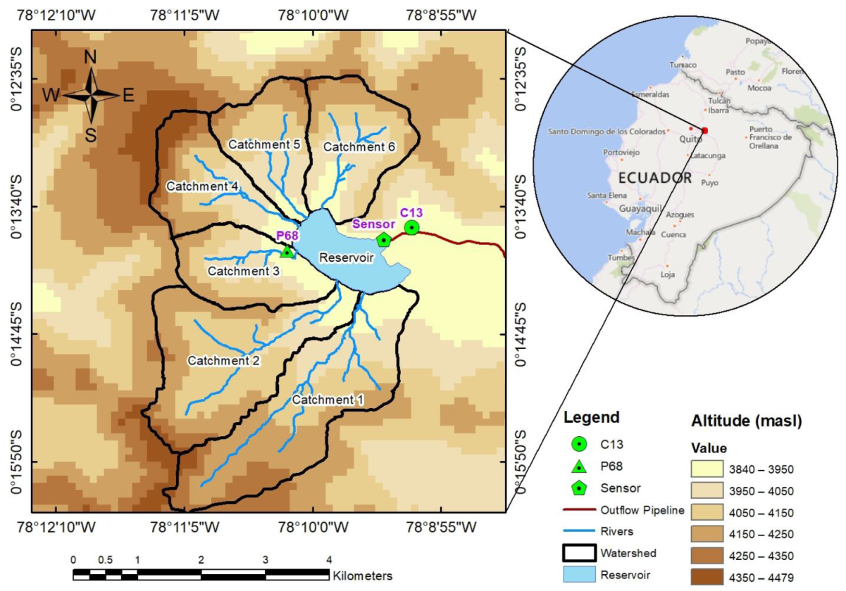
2.1. Area of Study

The Salve Faccha dam is a hydraulic structure of the Papallacta system located in the Andean part of northern Ecuador (Figure 1). It stores water for consumption purposes for Quito’s northern parishes, which house more than 300,000 users [26]. These parishes comprise Nayón, Zámbiza, Llano Chico, Pomasqui, San Antonio, Calderón, Pifo, Puembo, Yaruquí, Checa, and the area around the airport of the capital city. The dam has a maximum elevation of 3950 m above sea level, holds a maximum volume of 10,500,000 m³, and is located within the Oyacachi and Papallacta parishes in the province of Napo within the Cayambe-Coca Ecological Reserve [27].

The Salve Faccha dam is located on a high Andean plateau, as its altitude ranges between 4000 and 4500 m above sea level. The area belongs to the Bioclimatic region of Páramo Lluvioso because it has an annual rainfall of between 1000 and 1500 mm [28]. The daily temperature is highly variable, with a maximum range of 17 °C during the day and a minimum of −2 °C at night. There are three predominant plant covers: Herbaceous Páramo, Páramo de Páramo, and Shrub Páramo [29].

The reservoir receives runoff from six small catchments with a total extension of 14.24 km². The contributing catchments show a variable topography which includes steep terrain with medium slopes ranging from mild to moderate (14–29%). The highest percentage of the area has gentle slopes and volcano-sedimentary deposits [27]. The compactness indices slightly exceed one in all the catchments, which indicates longer concentration times. The shape factor of the catchments is less than 1, which denotes a slight elongation and thus a lower incidence of floods influenced by the shape.

In terms of data availability, daily rainfall and water levels data are available from 1 January 2012 to 31 December 2019 from stations P68 and C13 (Figure 2). These data series were provided by the Department of Water Resources of the Empresa Pública Metropolitana de Agua Potable y Saneamiento de Quito (EPMAPS). It should be noted that within the reservoir area, there are three hydrometric stations installed; however, they were not used in this study because they were recently installed, so there is limited information to be used as input for the DL models. Precipitation in the area is present throughout the year. Most rainfall in the region occurs between April and July.

2.2. Generalities of Neural Networks and ANFIS

Currently, there are several artificial intelligence techniques that can be applied to forecast the water level within reservoirs [30]. For the present research, neural networks were used because they are models that can reliably solve non-linear problems than traditional methods such as the moving average model or the autoregressive moving average model [31,32]. At the same time, neural networks are simple enough to be interpreted by the technicians and water practitioners who handle the reservoir. On the other hand, ANFIS was used because it is a more complex model than the high-performance neural networks, and it has the ability to handle the uncertainty of hydrological and climatic processes [33]. It has been shown that ANFIS tends to perform better than neural networks for the prediction of reservoir water levels [34]. However, its training and interpretation is usually more complex compared to neural networks. Nevertheless, previous research shows that both models have successfully been applied to forecast reservoir levels on a daily basis [35,36].

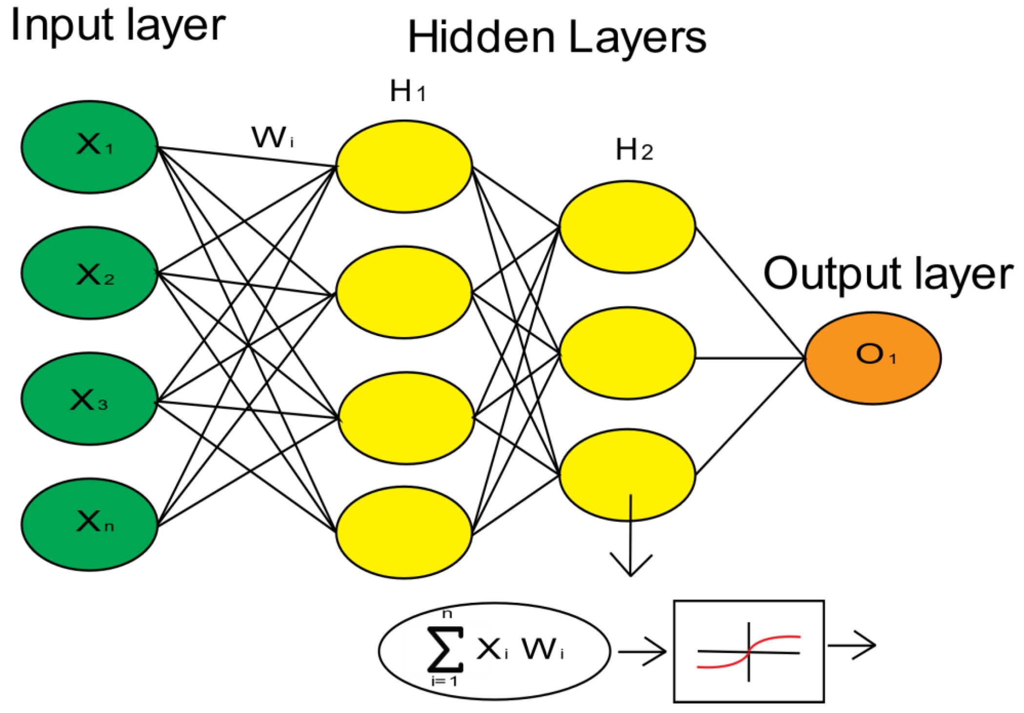
2.2.1. Neural Networks

A feed-forward neural network is a closed complex network made of several simple nodes that simulate the neural structure of the human brain. Typically, it consists of three connected parts or layers: the input layer, the hidden layer where the neurons are located, and the output layer [37], as shown in Figure 3. When using a neural network, the inputs in the first layer are multiplied by the weights (w_i) of the connections, which determine their importance. A summation of these multiplications is conducted within a neuron, and a bias of the node is then added. The result of each neuron is determined from the sum weight of all its inputs or nodes that pass through a non-linear function called the activation function, determining the level of activation. The most used transfer function is the sigmoidal (tan-sigmoid) function, as shown in the graph.

One of the most significant benefits of neural networks is their ability to learn patterns in data from the training process by modifying the weight of the networks’ connections and neuron bias by comparing model inputs and outputs. For supervised training models, a training algorithm (such as the backpropagation type) is used to minimize the output error when comparing the resulting value with the real one for each iteration of weight adjustment in a process called an epoch [37]. For a more detailed explanation of neural networks, we recommend reviewing [1,38].

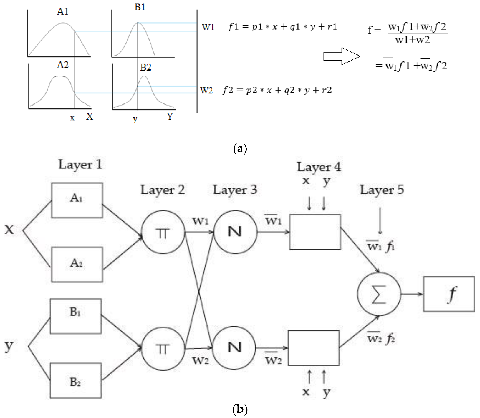
2.2.2. Functioning of ANFIS Model

Adaptive neuro-fuzzy inference system or ANFIS is an information processing model that uses fuzzy logic in an interconnected system that is trained with a supervised training system [39]. ANFIS combines the best of fuzzy logic, combining a system of rules that represent expert knowledge with the ability of NNs to be trained to capture the relationships between inputs and outputs. Decision rules are created through the use of expert knowledge or patterns and trends in data series. Despite this, the computational cost and training time is relatively high, especially in the training phase.

In order to simplify the explanation of how ANFIS function, let us have a two-input (“x” and “y”) model with one output, “z” for fuzzy Sugeno architecture. The typical model of an if-then rule of fuzzy logic is [34]:

Rule 1: If “x” is A₁ and “y” is B₁, then: f₁ = p₁*x + q₁*y + r₁;

Rule 2: If “x” is A₂ and “y” is B₂, then: f₂ = p₂*x + q₂*y + r₂.

A₁ and A₂ are the membership functions (MF) of inputs x, y, p_i, q_i, and r_i are linear parameters of the output function f as observed in Figure 4a.

ANFIS models consist of five layers or phases consisting of [40] (1) fuzzification, (2) the rules phase, (3) the normalization phase, (4) the de-fuzzification phase, and (5) the overall output phase (Figure 4b).

In the first layer, the inputs are transformed using the membership functions.

Li₁ = μ_Ai (x) for i = 1, 2 or Li₁ = μ_Bi−2 (y) for i = 3, 4

(1)

Ai and Bi represent the transfer function, and Ai (or Bi−2) is a fuzzy set associated with this node characterized by the transfer function shape. In general, the Gaussian function is used due to its concise notation and smoothness. These transfer functions show the decision thresholds of a variable on a scale from 0 to 1, defined by the following equation, where {a_i, b_i, c_i} are the parameters that define the form of the transfer functions in Equation (2):

$${\mu }_{Ai}=\frac{1}{1+{\left|\frac{x-c_i}{a_i}\right|}^{2b_i}}\hspace{1em}\hspace{1em}{\mu }_{Bi-2}=\frac{1}{1+{\left|\frac{y-c_i}{a_i}\right|}^{2b_i}}$$

(2)

In the second layer, the firing strength of the rules (w_i) is determined, for which the resulting values of the previous layer are multiplied, giving adjusted nodes. Each node represents the firing strength of each rule.

Li₂ = w_i = μ_Ai (x) μ_Bi (y)  i = 1, 2 k = 1, …, 4

(3)

Normalization, which divides the fire strength that is obtained per layer by the sum of all the connection weights is conducted in the third layer.

$${\mathrm{Li}}_3=w_i=\frac{w_1}{{{\displaystyle \sum }}_{k=1}^{4}wk}\hspace{1em}\hspace{1em}\hspace{1em}\hspace{1em}\hspace{1em}\hspace{1em}i=1,\dots ,4$$

(4)

In the fourth layer, the result of the previous layer is multiplied by multiple linear equations, which represent the rule systems of the Sugeno type ANFIS model defined above [1].

Li₄ = Li₃ × f_i = w_i (p₁*x + q₁*y + r₁)   i = 1, …, 4

(5)

where Li₄ is the fourth layer output, f_i is multiple linear equations, Li₃ is the third layer output, p, q, r are the multiple linear equation parameters, and x_i and y_i are the inputs of the membership degree.

In the fifth layer, all of the outputs of the fourth layer are added, giving the final results. The model can be trained using the hybrid-type learning algorithm, which combines least-squares estimators and the descending gradient method [39].

One disadvantage of traditional ANFIS-type models is their complex and demanding modeling when using more than six input variables due to the substantial increase in conditionals [41]. For example, for a ten-input model with three membership functions, each could have a total of 59,049 conditionals. Increasing the number of conditionals also increases the training time of the model due to the high complexity, which comes with the risk of obtaining unsatisfactory validation results. One solution is using data clustering techniques to separate large data series into groups where their behavior is similar. Groups of variables are obtained and activated by approximating them to the center of a radio cluster [42]. There are several clustering techniques such as c-means clustering [43], mountain clustering [44], G-K fuzzy clustering [45] and subtractive clustering [46]. Each grouping has a weight determined by the center of the clustering.

2.3. Data Pre-Processing

2.3.1. Quality Control of Data

A homogeneity test was performed, which determined the significant trend changes in the data due to measurement errors that include sensor failures and station position changes. The statistical program Rh test V3 was used based on the penalized maximal t-test for precipitation series and reservoir level to find statistically significant change points [47]. A reliability of 95% was used for the test as it was the most reliable, and the presence of type 1 change points were not considered homogeneous data [48].

Deterministic methods were used to fill in the missing precipitation data. First, the correlation between stations was determined, and a polynomial line of tendency was then fitted to the data. The missing data were filled in according to the highest correlation with the closest stations [49]. The moving mean method was used with a six-day moving window [50] and filled in using the average of the intermediate values with the MATLAB outlier tool to correct outliers.

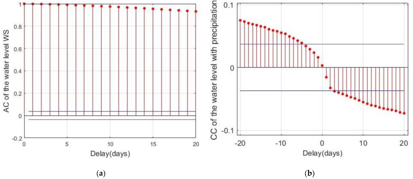
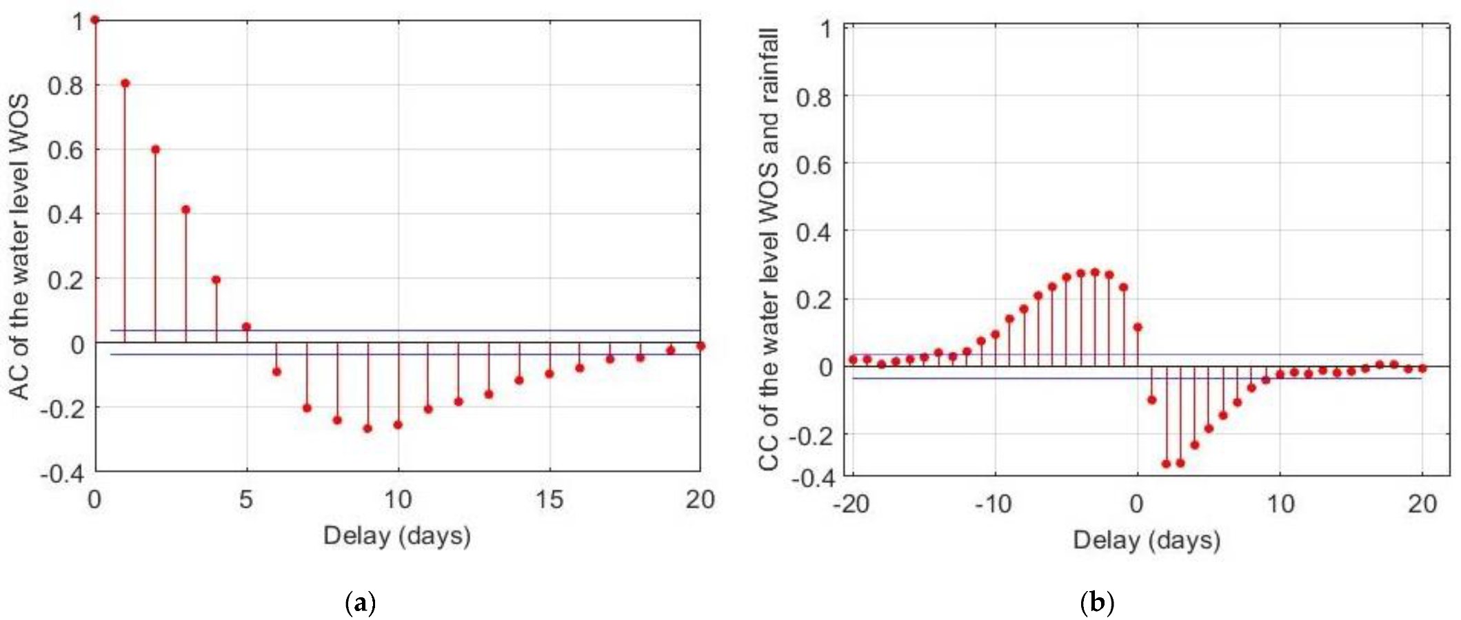
2.3.2. Determination of Predictors and Delay as Input

The model input and delay days were selected using the autocorrelation and cross-correlation between variables. These methods were selected because they are frequently used and for their excellent performance in hydrology models [21,51,52]. Generally, the graph measures the linear relationship between lagged values in a time series. Delay days that do not fall within a confidence limit (in this study, 95%) have some significant relationship and are not a statistical fluke. In case of encountering a seasonality when using a Fuller Dicker test (which makes it difficult to detect the number of delays in the graph), the seasonality will be removed from the subtraction of a series of mobile means for a better reading of the graph.

2.3.3. Neural Network and ANFIS Models Configuration

The use of cross-validation in machine learning model development is common. This methodology consists of dividing the data into three different groups called training, validation, and testing. The first is applied to train the neural network in different configurations. The second group validates the performance of the neural network during training. Finally, the test group is used to test the model using new information that the model has not processed before. There are 2920 rainfall and water level observations, which were split into 70% for the training, 15% for validation, and 15% for test models (November 2018 to December 2019).

An input–output neural network available in the MATLAB neural net time series library was used in this study. In these models, the number of delay days used (x-n) is specified to determine the output of the target. The inputs were normalized in a range of (−1, 1) in order to avoid certain inputs having more weight than others. The tangential-sigmoid type was used to capture the normalization range of the data. The output equation is linear because it allows the interpretation of higher values of the reservoir level not used in the training phase. The Levenger–Marquart training algorithm is used due to having a low training time with satisfactory results. The neural network architecture has been defined by trial and error based on the minimization of the training and validation error for an optimal generalization of the model results [53].

For ANFIS, the subtractive clustering method was used with an initial acceptance radius of 0.5 to 0.8 with a maximum of 500 iterations of training and validation in the Matlab fuzzy library. The same inputs from the neural networks were used for the model. However, the number of delay days was limited to four days due to the increased training time. The Gaussian transfer function was used as it is the only one in the ANFIS algorithm for subtractive clustering.

2.3.4. Model Performance Criteria

The correlation coefficient (CC), RMSE (root mean square error), and the Nash–Sutcliffe (NS) efficiency test were used to measure the performance of the models due to their regular use in hydrological modeling [54] (Equations (5)–(7)). In general, the closer the CC and NS values are to 1, and the closer the RMSE is to 0, the better the model is at predicting. Models will be considered models of high precision if the CC and NS values are more significant than 0.9, and the RMSE value is less than 0.1 [55]. Taylor diagrams were used to make a multi-objective evaluation, which are graphic representations between the modeled and observed series of three statistical metrics: Pearson’s correlation coefficient, the root mean square error (RMSE), and the standard deviation. Model performance was also evaluated for the dry and rainy seasons. The dry season was considered to be from April to June. The maximum and the minimum water levels of the reservoir were also observed and were consistent during the indicated dry and wet seasons.

$$CC=\sqrt{\frac{{({{\displaystyle \sum }}_{i=1}^N\left(X_i-\overline{X}\right)\times \left(Y_i-\overline{Y}\right))}^2}{{{\displaystyle \sum }}_{i=1}^N{\left(X_i-\overline{X}\right)}^2\times {{\displaystyle \sum }}_{i=1}^N{(Y_i-\overline{Y})}^2}}$$

(6)

$$NS=1-\frac{{{\displaystyle \sum }}_{i=1}^N{\left(X_i-Y_i\right)}^2}{{{\displaystyle \sum }}_{i=1}^N{\left(X_i-\overline{X}\right)}^2}$$

(7)

where X_i is the actual value of reservoir water level, X is the mean of the actual value, Y_i is the prediction of reservoir water level, and Y is the mean of the prediction of the actual value of the water level.

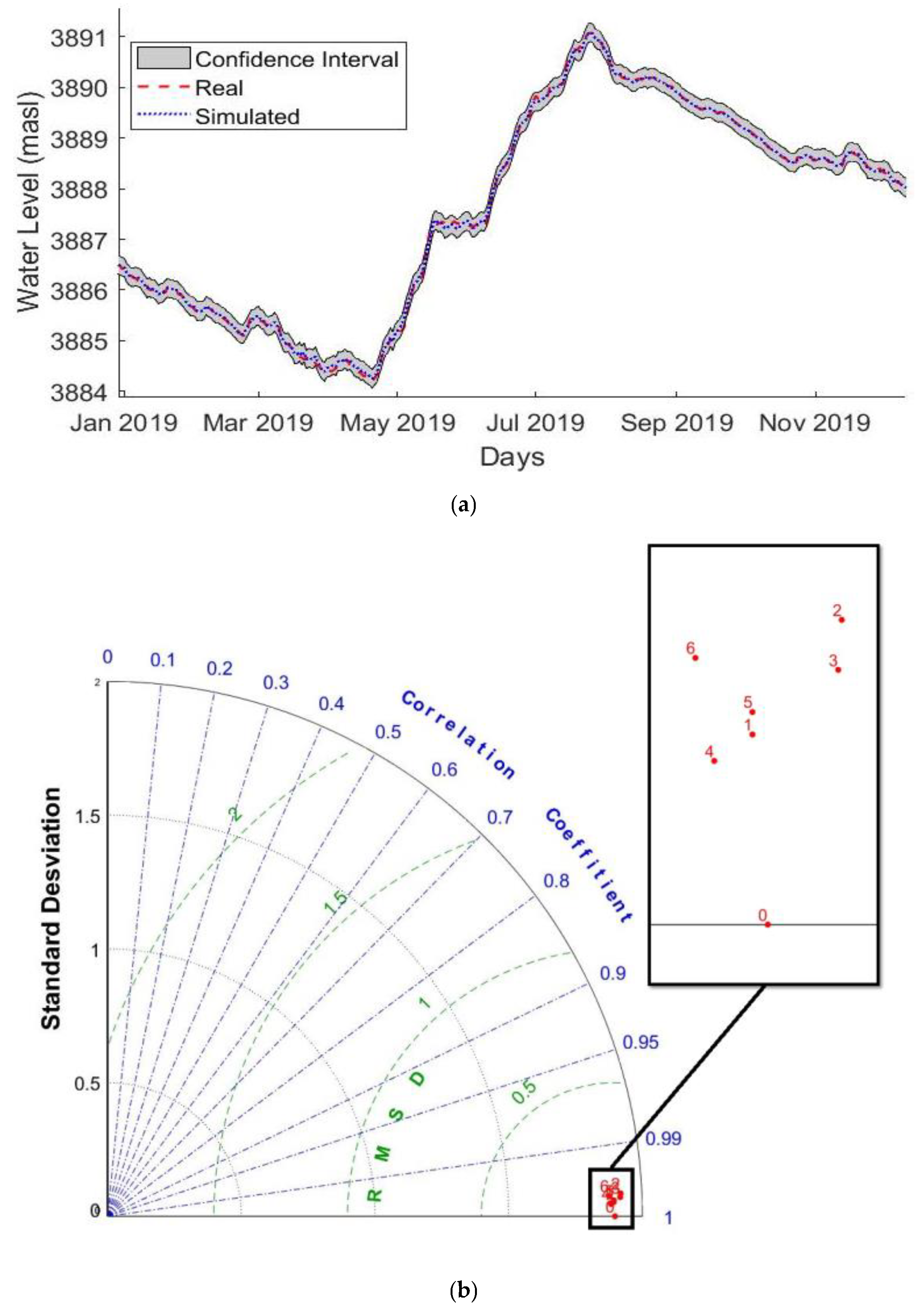
2.4. Prediction Confidence Intervals Development

The Bootstrap percentile-t method was used to determine the confidence intervals of the predictions. This method was selected because it was applied to generate the confidence intervals for the reservoir level forecasts [42] and the confidence intervals for the monthly precipitation predictions [56]. The t-percentile method generates t-values of the classical theory of confidence interval generation. It is assumed that for the Bootstrap samples, the data series, and each sample the statistical parameter of interest θ is determined (which in the case of the investigation are the predictions of the reservoir level), and the standard error of the parameter of the samples is estimated [57]. For a confidence interval t with a reliability of 95%, the construction is as follows: θ = predicted value, se = the Bootstrap standard error, and $t_{n-1}^{\left(\frac{\alpha }{2}\right)}$ = the alpha value of the percentiles (Equation (8))

$$\left[\widehat{\theta }-t_{n-1}^{\left(\frac{\alpha }{2}\right)}\times \widehat{se}, \widehat{\theta }+t_{n-1}^{\left(1-\frac{\alpha }{2}\right)}\times \widehat{se}\right]$$

(8)

3. Results and Discussion

3.1. Selection of Predictors

Adequate identification of the predictors of a model is essential for its proper functioning, in some cases showing even greater importance than the selection of the best model architecture [58]. The autocorrelation between the variables does not exhibit a useful pattern to determine the maximum delay period due to the seasonality, as observed in Figure 5a. Equally important, the cross-correlation graph between precipitation and the trending level (Figure 5b) shows a low correlation (<0.1) and is close to the limit of significant error represented by the blue lines. Therefore, the variable of rainfall and water level with seasonality has little relationship at the daily time steps. For this reason, a more in-depth analysis of the time series relationship was developed.

The residuals of the water level time series were calculated to make the model non-seasonal. The process was conducted to better determine the delay. The new data were obtained from the subtraction between the level and a 20-day moving average, capturing the seasonality. Figure 6a shows the autocorrelation of the non-stationary level where we have 18 days without entering the significant error, which is represented by the blue line. Regarding the cross-correlation with rainfall (Figure 6b), it increases to a maximum of 0.3. Since the maximum autocorrelation of the graphic is 0.3, it could be inferred that precipitation might not be the most crucial variable in NN and ANFIS models. In conclusion, 13 lag days were selected as input (see Figure 6b).

Precipitation may be a poor predictor within the ANFIS and NN models. The study area is still characterized by a poor distribution of hydrometeorological stations. The public water company, EPMAPS, is in charge of the hydrological monitoring of the area, and it is currently installing additional water monitoring stations. Therefore, future hydrological models will have more precipitation and discharge data availability. Moreover, the Andean páramos have high climatic variability [59], which, together with the limited water sampling stations, complicates the estimation of precipitation input for the Salve Faccha reservoir. Moreover, in the northern Andean paramo, soil properties have been documented as highly porous with high organic matter content, so they have a buffer capacity for precipitation events, a high-water retention capacity within the soil reservoir, and a strong regulating capacity of baseflow [60]. Due to soil properties, it is unlikely that water levels within the reservoir are highly responsive to precipitation events.

Through trial and error, it was determined that the data series of the water level with filters should be included to increase the models’ recommended performance [61]. Six inputs were selected: (1) the water level with seasonality, (2) the water level moving average, (3) the non-seasonality water level, (4), the water level without linear trend, and (5 and 6) the rainfall series of stations P68 and C13. Due to the low cross-correlation of rainfall with the water level, models with and without rainfall were tested to determine the impact of the inclusion and exclusion of these variables on their performance.

3.2. Neural Network Results

Table 1. The general performance of neural networks models with rainfall and without rainfall as input.

Forecast	Correlation		RMSE		NS		Delay (Days)		Nodes
	WP	WOP	WP	WOP	WP	WOP	WP	WOP	WP	WOP
t + 1	0.9992	0.999	0.076	0.053	0.998	0.999	13	13	15	20
t + 2	0.9996	0.999	0.056	0.096	0.999	0.997	13	13	15	30
t + 3	0.999	0.999	0.093	0.076	0.998	0.998	11	10	20	20
t + 4	0.9993	1.000	0.076	0.046	0.998	0.999	11	12	20	20
t + 5	0.9993	0.999	0.095	0.062	0.998	0.999	13	10	15	15
t + 6	0.9994	0.999	0.066	0.075	0.999	0.998	13	8	25	15

Symbology. W = models with precipitation, WOP = models without precipitation, RMSE = root mean square error, NS = Nash–Sutcliffe efficiency.

shows the performance metrics for the neural network forecasts over 1 to 6 days. No improvement or worsening is observed when comparing the results with/without including rainfall as input according to performance metrics. The two types of models have a high correlation with a Nash index very close to one, with an RMSE less than 0.1. However, networks with no precipitation input require fewer lag days for the five- and six-day predictions. Therefore, they are accepted as superior because they need less information to obtain equally satisfactory results. This result supports the autocorrelation values indicated in Section 3.1 when considering precipitation as a low-impact variable for water level predictions. For example, Hussain and collaborators only used precipitation to predict the water level of the next day, obtaining errors of up to 44% during the test period [11].

The best-performing models without rainfall contain 15–20 neurons with a single hidden layer, except for the two-day prediction model, which required 30 nodes for the best results. Based on performance metrics, the best model is the four-day prediction model with an RMSE of 0.046 with a maximum of 0.18 m with a 95% confidence interval, followed by the one-day prediction model with an RMSE of 0.053 (Figure 7a). The errors of the other days are very close, with RMSE less than 0.1. As in other recent studies [62], our results tend to worsen as the difference between the input days and the days to forecast increases, however, these high-performance results can be maintained. Equally important, the best performance models are obtained with simple model architectures with fewer nodes, similar to the study by Piri and Rezaei, who predicted reservoir levels with a single hidden layer with less than 10 nodes and inputs from past levels in 2016 [19].

The performance of the models is observed in the Taylor diagram, where zero represents the actual data series, and the numbers are the forecast days of each selected neural network (Figure 7b). However, subsequent studies should evaluate the average efficiency of the same architecture to avoid selecting models optimized in local minima, as they have low generalizability and present poor results from data other than those used for calibration.

3.3. ANFIS Results

The results were split into models with rainfall (WP) and models without precipitation (WOP) in

Table 2. General performance parameters of ANFIS models with rainfall and without rainfall as input.

Forecast	Correlation		RMSE		ns		Delay (Days)
	WP	WOP	WP	WOP	WP	WOP	WP	WOP
t + 1	0.9996	0.9996	0.0517	0.0505	0.9992	0.9993	3	3
t + 2	0.9992	0.9992	0.0756	0.0745	0.9984	0.9984	3	4
t + 3	0.9989	0.9990	0.0880	0.0820	0.9978	0.9981	3	4
t + 4	0.9989	0.9990	0.0884	0.0807	0.9978	0.9981	3	4
t + 5	0.9990	0.9990	0.0837	0.0769	0.9980	0.9981	3	4
t + 6	0.9991	0.9992	0.0780	0.0737	0.9983	0.9981	3	4

Symbology. WP = models with precipitation, WOP = models without precipitation, RMSE = root mean square error, NS = Nash–Sutcliffe efficiency.

. Information from the various three days was needed to obtain the best results to predict the reservoir level for the models with precipitation. Despite this, the one and two-day predictions were more similar to the naive-type predictions. These models are characterized by the replication of the previous value as the prediction value. This result is similar to the neural network models with a three-day delay. Therefore, it can be concluded that three and four days of delay input is not enough information to generate predictive t + 1 and t + 2 models for neural networks and ANFIS.

Slightly better performance is observed with a shorter training and validation time due to having fewer entries to cluster despite having entries spanning up to four days. As with previous neural network models, it can be concluded that the precipitation variable is not needed to forecast the reservoir level for up to six days. Despite this, the one-day forecast and two-day forecast models are similar to the naive models. The best model for ANFIS was for t + 6, with an RMSE of 0.0737 with four days of delay (Figure 8a), which agrees with the ability of the models to make predictions at different time periods when determining reservoir water level predictions up to three days into the future, as obtained by [20]. The Taylor diagram of all of the ANFIS models presents a highly accurate performance that is very close to the actual data series because they are grouped (Figure 8b).

Table 3. Performance parameters of NN and ANFIS models in seasonality.

Model	Forecast	Rainy Season			Dry Season
		Correlation	RMSE	NS	Correlation	RMSE	NS
Neural Networks	t + 1	0.9996	0.0653	0.9992	0.9997	0.0424	0.9994
	t + 2	0.9989	0.105	0.9979	0.9994	0.0595	0.9988
	t + 3	0.9987	0.118	0.9973	0.9992	0.0674	0.9984
	t + 4	0.9987	0.1159	0.9974	0.9992	0.0697	0.9983
	t + 5	0.9988	0.1075	0.9978	0.9992	0.0635	0.9986
	t + 6	0.9989	0.1092	0.9977	0.9993	0.0674	0.9984
ANFIS	t + 1	0.9995	0.077	0.9988	0.9998	0.0402	0.9995
	t + 2	0.9983	0.1351	0.9965	0.9996	0.0744	0.9981
	t + 3	0.999	0.1082	0.9977	0.9996	0.0579	0.9989
	t + 4	0.9997	0.0659	0.9992	0.9998	0.0342	0.9996
	t + 5	0.9992	0.1146	0.9974	0.9996	0.0523	0.9991
	t + 6	0.9988	0.0888	0.9985	0.9995	0.0472	0.9992

Symbology. RMSE = root mean square error, NS = Nash–Sutcliffe efficiency.

indicates the performance of the neural networks and ANFIS by season. A good performance can be observed in the rainy and dry seasons. The error in the rainy season is greater in the months when the dam level begins to increase at the beginning of the season because this period has been the wettest month since 2012, as seen in the participation heat map in the graph in Figure 9. An increase in the DL models is expected due to incorrect generalizations when entering values with different trends or values that are higher than those used for the training period [1]. Furthermore, the rainy season shows greater variability than the dry season, which makes it difficult for the model to produce a better forecast. Despite this, the models can generalize and predict with a low error frequency, mainly due to the low influence of rainfall on the variability of the water level over time. This result is possible with the linear transfer function in the final layer of the neural network.

4. Conclusions

Prediction models for the water levels of the Salve Faccha dam were generated up to six days in advance using neural network models and ANFIS models. The neural network models required up to 13 days of delay and architectures of less than 30 nodes with satisfactory results. On the contrary, the ANFIS models were able to obtain similar results using up to four days of previous information. However, t + 1 and t + 2 are similar to naïve models because they do not have the necessary delay information.

Rainfall inputs were not fundamental to making predictions for both the NN and ANFIS models. This may be due to primary by the inadequate spatial distribution of the precipitation stations, the buffer effect of the large reservoir, soil properties, among other factors. For future studies, we recommend testing new models that incorporate inflow and precipitation data. We also recommend forecasting water levels by applying more sophisticated models such as extreme learning machines or genetic programming.

In both models, good results were obtained for the dry season, with slightly worse results in the forecasts for the rainy season, with RMSE > 0.13 for some models. This occurred because the monthly rainfall during this period has been the highest it has ever been since 2012, so there was no data in the training period for such climatic events.

Likewise, confidence intervals using the percentile-t method were generated to have forecasts with an uncertainty reduction that DL models may have with a maximum of 0.18 m with a confidence of 95%. There was a low amplitude that was mainly produced by the high prediction performance of the models with real observations of the water level of the dam. Thus, it can be concluded that ANFIS models are superior to neural network models because they require less prior information to conduct projections of the future.

References

1. Oyebode, O.; Stretch, D. Neural network modeling of hydrological systems: A review of implementation techniques. Nat. Resour. Model. 2018, 32, e12189. [Google Scholar] [CrossRef] [Green Version]
2. Halff, A.H.; Halff, H.M.; Azmoodeh, M. Predicting runoff from rainfall using neural network. In Engineering Hydrolgy; American Society of Civil Engineers: New York, NY, USA, 1993; pp. 760–765. [Google Scholar]
3. Zhu, M.-L.; Fujita, M.; Hashimoto, N. Application of neural networks to runoff prediction. In Climate Change Impacts on Water Resources, 3rd ed.; Panu, A., Singh, U., Eds.; Springer: Dordrecht, The Netherlands, 1994; Volume 10, pp. 205–216. [Google Scholar]
4. Govindaraju, R. Artificial neural networks in hydrology. II: Hydrologic applications. J. Hydrol. Eng. 2000, 5, 124–137. [Google Scholar] [CrossRef]
5. Herrera, M.; Torgo, L.; Izquierdo, J.; Pérez-García, R. Predictive models for forecasting hourly urban water demand. J. Hydrol. 2010, 387, 141–150. [Google Scholar] [CrossRef]
6. Zubaidi, S.; Al-Bugharbee, H.; Ortega-Martorell, S.; Gharghan, S.; Olier, I.; Hashim, K.; Al-Bdairi, N.; Kot, P. A Novel Methodology for Prediction Urban Water Demand by Wavelet Denoising and Adaptive Neuro-Fuzzy Inference System Approach. Water 2020, 12, 1628. [Google Scholar] [CrossRef]
7. Azad, A.; Karami, H.; Farzin, S.; Mousavi, S.-F.; Kisi, O. Modeling river water quality parameters using modified adaptive neuro fuzzy inference system. Water Sci. Eng. 2019, 12, 45–54. [Google Scholar] [CrossRef]
8. García, I.; Rodríguez, J.G.; Lopez, F.; Tenorio, Y.M. Transporte de Contaminantes en Aguas Subterráneas mediante Redes Neuronales Artificiales. Inf. Tecnológica 2010, 21, 79–86. [Google Scholar] [CrossRef] [Green Version]
9. Nalavade, J.E.; Murugan, T.S. HRNeuro-fuzzy: Adapting neuro-fuzzy classifier for recurring concept drift of evolving data streams using rough set theory and holoentropy. J. King Saud Univ. Comput. Inf. Sci. 2018, 30, 498–509. [Google Scholar] [CrossRef] [Green Version]
10. Peñas, F.J.; Barquín, J.; Snelder, T.H.; Booker, D.J.; Álvarez, C. The influence of methodological procedures on hydrological classification performance. Hydrol. Earth Syst. Sci. 2014, 18, 3393–3409. [Google Scholar] [CrossRef]
11. Hussain, W.; Ruhana, K.; Norwawi, N.M. Neural network application in reservoir water level forecasting and release decision. Int. J. New Comput. Archit. Appl. 2011, 1, 256–274. [Google Scholar]
12. Graf, W.L. Geomorphology and American dams: The scientific, social, and economic context. Geomorphology 2005, 71, 3–26. [Google Scholar] [CrossRef]
13. Monadi, M.; Samani, H.M.V.; Mohammadi, M. Optimal design and benefit/cost analysis of reservoir dams by genetic algorithms case study: Sonateh Dam, Kordistan Province, Iran. Int. J. Eng. 2016, 29, 481–488. [Google Scholar] [CrossRef]
14. Hejazi, M.I.; Cai, X.; Ruddell, B. The role of hydrologic information in reservoir operation—Learning from historical releases. Adv. Water Resour. 2008, 31, 1636–1650. [Google Scholar] [CrossRef]
15. McManamay, R.A. Quantifying and generalizing hydrologic responses to dam regulation using a statistical modeling approach. J. Hydrol. 2014, 519, 1278–1296. [Google Scholar] [CrossRef] [Green Version]
16. Loucks, D.P.; Van Beek, E. Water Resource Systems Planning and Management: An Introduction to Methods, Models, and Applications; Springer International Publishing: Basel, Switzerland, 2017. [Google Scholar]
17. Martinez, L.; Santos, F. Generación de Modelos Estadísticos Utilizando Redes Neuronales Y Series de Tiempo Para el Pronóstico de Los Niveles del Reservorio de la Presa Hidroeléctrica Cerrón Grande de el Salvador; Universidad de EL Salvador: Santa Ana, El Salvador, 2019. [Google Scholar]
18. Solomatine, D.P.; Torres, A. Neural network approximation of a hydrodynamic model in optimizing reservoir operation. In Proceedings of the 2nd International Conference on Hydroinformatics, Zurich, Switzerland, 9–13 September 1996. [Google Scholar]
19. Piri, J.; Rezaei, M. Prediction of water level fluctuations of chahnimeh reservoirs in zabol using ANN, ANFIS and Cuckoo Optimization Algorithm. Iran. J. Health Saf. Environ. 2016, 4, 706–715. [Google Scholar]
20. Chang, F.-J.; Chang, Y.-T. Adaptive neuro-fuzzy inference system for prediction of water level in reservoir. Adv. Water Resour. 2006, 29, 1–10. [Google Scholar] [CrossRef]
21. Üneş, F.; Demirci, M.; Taşar, B.; Kaya, Y.Z.; Varçin, H. Estimating Dam Reservoir Level Fluctuations Using Data-Driven Techniques. Pol. J. Environ. Stud. 2019, 28, 3451–3462. [Google Scholar] [CrossRef]
22. Yates, D.; Sieber, J.; Purkey, D.; Huber-Lee, A. WEAP21—A Demand-, Priority-, and Preference-Driven Water Planning Model. Water Int. 2005, 30, 487–500. [Google Scholar] [CrossRef]
23. Kangrang, A.; Prasanchum, H.; Hormwichian, R. Development of future rule curves for multipurpose reservoir operation using conditional genetic and tabu search algorithms. Adv. Civ. Eng. 2018, 2018, 6474870. [Google Scholar] [CrossRef] [Green Version]
24. Bazartseren, B.; Hildebrandt, G.; Holz, K.-P. Short-term water level prediction using neural networks and neuro-fuzzy approach. Neurocomputing 2003, 55, 439–450. [Google Scholar] [CrossRef]
25. Yang, S.; Yang, D.; Chen, J.; Zhao, B. Real-time reservoir operation using recurrent neural networks and inflow forecast from a distributed hydrological model. J. Hydrol. 2019, 579, 124229. [Google Scholar] [CrossRef]
26. INE. Población Por Sexo, Según Provincia, Parroquia y Cantón de Empadronamiento; INE: Quito, Ecuador, 2011.
27. EPMAPS. Caracterización de Las Microcuencas Aportantes al Embalse Salve Faccha del Sistema Papallacta; EPMAPS: Quito, Ecuador, 2016. [Google Scholar]
28. Cañadas, L. El Mapa Bioclimático y Ecológico del Ecuador; MAF-Pronareg: Quito, Ecuador, 1983.
29. Baquero, F.; Sierra, R.; Ordóñez, L.; Tipán, M.; Espinosa, L.; Belen Rivera, M.; Soria, P. La Vegetación de los Andes del Ecuador; EcoCiencia/CESLA/EcoPar/MAG SIGAGRO/CDC-JATUN SACHA/División Geográfica—IGM: Quito, Ecuador, 2004. [Google Scholar]
30. Zhu, S.; Lu, H.; Ptak, M.; Dai, J.; Ji, Q. Lake water-level fluctuation forecasting using machine learning models: A systematic review. Environ. Sci. Pollut. Res. 2020, 27, 44807–44819. [Google Scholar] [CrossRef] [PubMed]
31. Vaziri, M. Predicting caspian sea surface water level by ANN and ARIMA Models. J. Waterw. Port Coast. Ocean Eng. 1997, 123, 158–162. [Google Scholar] [CrossRef]
32. Altunkaynak, A. Forecasting Surface Water Level Fluctuations of Lake Van by Artificial Neural Networks. Water Resour. Manag. 2006, 21, 399–408. [Google Scholar] [CrossRef]
33. Nayak, P.; Sudheer, K.; Rangan, D.; Ramasastri, K. A neuro-fuzzy computing technique for modeling hydrological time series. J. Hydrol. 2004, 291, 52–66. [Google Scholar] [CrossRef]
34. Dalkiliç, H.Y.; Hashimi, S.A. Prediction of daily streamflow using artificial neural networks (ANNs), wavelet neural networks (WNNs), and adaptive neuro-fuzzy inference system (ANFIS) models. Water Supply 2020, 20, 1396–1408. [Google Scholar] [CrossRef] [Green Version]
35. Yarar, A.; Onucyıldız, M.; Copty, N.K. Modelling level change in lakes using neuro-fuzzy and artificial neural networks. J. Hydrol. 2009, 365, 329–334. [Google Scholar] [CrossRef]
36. Kisi, O.; Shiri, J.; Nikoofar, B. Forecasting daily lake levels using artificial intelligence approaches. Comput. Geosci. 2012, 41, 169–180. [Google Scholar] [CrossRef]
37. Svozil, D.; Kvasnicka, V.; Pospichal, J. Introduction to multi-layer feed-forward neural networks. Chemom. Intell. Lab. Syst. 1997, 39, 43–62. [Google Scholar] [CrossRef]
38. Abrahart, R.; Kneale, P.; See, L.M. Neural Networks for Hydrological Modeling; A.A.Balkema Publishers: London, UK, 2004. [Google Scholar]
39. Ata, R.; Kocyigit, Y. An adaptive neuro-fuzzy inference system approach for prediction of tip speed ratio in wind turbines. Expert Syst. Appl. 2010, 37, 5454–5460. [Google Scholar] [CrossRef]
40. Shing, R.; Sun, C.-T.; Mizutani, E. Neuro-Fuzzy and Soft Computing: A Computional Approach to Learning a Machine Intelligence, 1st ed.; Prentice Hall: Englewood Cliffs, NJ, USA, 1997. [Google Scholar]
41. Khoshnevisan, B.; Rafiee, S.; Omid, M.; Mousazadeh, H. Development of an intelligent system based on ANFIS for predicting wheat grain yield on the basis of energy inputs. Inf. Process. Agric. 2014, 1, 14–22. [Google Scholar] [CrossRef] [Green Version]
42. Talebizadeh, M.; Moridnejad, A. Uncertainty analysis for the forecast of lake level fluctuations using ensembles of ANN and ANFIS models. Expert Syst. Appl. 2011, 38, 4126–4135. [Google Scholar] [CrossRef]
43. Bezdek, J.C.; Ehrlich, R.; Full, W. FCM: The fuzzy c-means clustering algorithm. Comput. Geosci. 1984, 10, 191–203. [Google Scholar] [CrossRef]
44. Yager, R.R.; Filev, D.P. Generation of Fuzzy Rules by Mountain Clustering. J. Intell. Fuzzy Syst. 1994, 2, 209–219. [Google Scholar] [CrossRef]
45. Sivaraman, E.; Arulselvi, S. Gustafson-kessel (G-K) clustering approach of T-S fuzzy model for nonlinear processes. In Proceedings of the 2009 Chinese Control and Decision Conference, Shanghai, China, 15–18 December 2009; pp. 791–796. [Google Scholar]
46. Chiu, S.L. Fuzzy Model Identification Based on Cluster Estimation. J. Intell. Fuzzy Syst. 1994, 2, 267–278. [Google Scholar] [CrossRef]
47. Wang, X.L.; Wen, Q.H.; Wu, Y. Penalized Maximal t Test for Detecting Undocumented Mean Change in Climate Data Series. J. Appl. Meteorol. Clim. 2007, 46, 916–931. [Google Scholar] [CrossRef]
48. Wang, X.L.; Yang, F. RHtestsV3 User Manual; Climate Research Division Atmospheric Science and Technology Directorate Science and Technology Branch, Environment Canada: Toronto, ON, Canada, 2010.
49. Campozano, L.; Sánchez, E.; Avilés, Á.; Samaniego, E. Evaluation of infilling methods for time series of daily precipitation and temperature: The case of the Ecuadorian Andes. MASKANA 2014, 5, 99–115. [Google Scholar] [CrossRef]
50. Blázquez-García, A.; Conde, A.; Mori, U.; Lozano, J.A. A review on outlier/anomaly detection in time series data. ACM Comput. Surv. 2020, 54, 1–33. [Google Scholar] [CrossRef]
51. Huang, W.; Foo, S. Neural network modeling of salinity variation in Apalachicola River. Water Res. 2002, 36, 356–362. [Google Scholar] [CrossRef]
52. Silverman, D.; Dracup, J.A. Artificial neural networks and long-range precipitation prediction in California. J. Appl. Meteorol. 2000, 39, 57–66. [Google Scholar] [CrossRef]
53. Maier, H.R.; Jain, A.; Dandy, G.C.; Sudheer, K. Methods used for the development of neural networks for the prediction of water resource variables in river systems: Current status and future directions. Environ. Model. Softw. 2010, 25, 891–909. [Google Scholar] [CrossRef]
54. Apaydin, H.; Feizi, H.; Sattari, M.T.; Colak, M.S.; Shamshirband, S.; Chau, K.-W. Comparative Analysis of Recurrent Neural Network Architectures for Reservoir Inflow Forecasting. Water 2020, 12, 1500. [Google Scholar] [CrossRef]
55. Chiew, F.; Stewardson, M.; McMahon, T. Comparison of six rainfall-runoff modelling approaches. J. Hydrol. 1993, 147, 1–36. [Google Scholar] [CrossRef]
56. Cowpertwait, P.S.P. Bootstrap confidence intervals for predicted rainfall quantiles. Int. J. Clim. 2001, 21, 89–94. [Google Scholar] [CrossRef] [Green Version]
57. Jung, K.; Lee, J.; Gupta, V.; Cho, G. Comparison of bootstrap confidence interval methods for gsca using a monte carlo simulation. Front. Psychol. 2019, 10, 2215. [Google Scholar] [CrossRef] [Green Version]
58. Bowden, G.J.; Dandy, G.C.; Maier, H.R. Input determination for neural network models in water resources applications. Part 1—background and methodology. J. Hydrol. 2005, 301, 75–92. [Google Scholar] [CrossRef]
59. Garreaud, R. The Andes climate and weather. Adv. Geosci. 2009, 22, 3–11. [Google Scholar] [CrossRef] [Green Version]
60. Buytaert, W.; Célleri, R.; De Bièvre, B.; Cisneros, F.; Wyseure, G.; Deckers, J.; Hofstede, R. Human impact on the hydrology of the Andean páramos. Earth-Sci. Rev. 2006, 79, 53–72. [Google Scholar] [CrossRef]
61. Banhatti, A.G.; Deka, P.C. Effects of Data Pre-processing on the Prediction Accuracy of Artificial Neural Network Model in Hydrological Time Series. In Climate Change Impacts on Water Resources; Springer: Cham, Switzerland, 2016; pp. 265–275. [Google Scholar]
62. Londhe, S. Towards predicting water levels using artificial neural networks. In Proceedings of the OCEANS 2009-EUROPE, Bremen, Germany, 11–14 May 2009; pp. 1–6. [Google Scholar] [CrossRef]
Figure 1. Location of the Salve Faccha dam on the northern Ecuadorian Andes.
Water 13 02011 g001
Figure 2. Time series of rainfall at the P68 station and reservoir’s water levels in meters above sea level.
Water 13 02011 g002
Figure 3. Neural Network structure.
Water 13 02011 g003
Figure 4. The architecture of an ANFIS model. (a) interpretation of the inputs in the membership functions; (b) graphical representation of an ANFIS system.
Water 13 02011 g004
Figure 5. Water level autocorrelation (a) and rainfall cross-correlation with P68 (b). Symbology: AC = Autocorrelation, WS = with seasonality, CC = cross-correlation.
Water 13 02011 g005
Figure 6. Water level autocorrelation (a) and cross-correlation of precipitation (b). Symbology: AC = Autocorrelation, WOS = without seasonality, CC = cross-correlation.
Water 13 02011 g006
Figure 7. Graphic results of the best prediction results for NN. (a) Comparison of the best model (t + 4) with its confidence interval. (b) Taylor diagram. In this diagram, point 0 is real observation data, and 1 to 6 are the models from t + 1 to t + 6 respectively, as shown in Table 1.
Water 13 02011 g007
Figure 8. Graphic results of the best prediction results for ANFIS. (a) Comparison of the best model (t + 4) with its confidence interval. (b) Taylor diagram. In this diagram, point 0 is real observation data, and 1 to 6 are the models from t + 1 to t + 6 respectively, shown in Table 2.
Water 13 02011 g008aWater 13 02011 g008b
Figure 9. Precipitation heat map of P68 station.
Water 13 02011 g009