
Analysis of the Flow Pattern and Flow Rectification Measures of the Side-Intake Forebay in a Multi-Unit Pumping Station

1
College of Hydraulic Science and Engineering, Yangzhou University, Yangzhou 225009, China
2
Egyptian Ministry of Water Resources and Irrigation, Imbaba 12666, Giza, Egypt
3
Key Laboratory of Fluid and Power Machinery, Ministry of Education, Chengdu 610039, China
4
Jiangsu Surveying and Design Institute of Water Resources Co., Ltd., Yangzhou 225127, China
5
Industrial and Systems Engineering Department, Faculty of Engineering, Misr University for Science and Technology (MUST), 6th of October City 12511, Giza, Egypt
*
Author to whom correspondence should be addressed.
Water 2021, 13(15), 2025; https://doi.org/10.3390/w13152025
Submission received: 1 July 2021
/
Revised: 23 July 2021
/
Accepted: 23 July 2021
/
Published: 24 July 2021
(This article belongs to the Section Hydraulics and Hydrodynamics)
Abstract
:To improve the problem of turbulence in the forebay of the lateral inlet pumping station, a typical lateral inlet pumping station project in Xuzhou, Jiangsu Province, China was taken as the research object. The forebay of the pumping station is a building connecting the river channel and the pumping station into the water tank. Based on the Reynolds-averaged Navier-Stokes (RANS) law and the k-ε turbulence model, the computational fluid dynamics method (CFD) technology compares and analyzes the numerical simulation with or without rectification measures for the forebay of the lateral intake pumping station when multiple units are operating. The three-dimensional model was created by SolidWorks modeling software and the numerical simulation simulated by CFX-ANSYS. To alter the flow pattern in the forebay of the pumping station, various rectification measures were chosen. Internal rectification flow patterns in the forebay under multiple plans, uniformity of flow velocity distribution in the measuring section, and vortex area reduction rates are investigated and compared. Based on the analysis and comparison of numerical simulation results, when the parabolic wall and some rectification piers are set significantly it improves the flow pattern of the forebay of the lateral inlet pumping station. It also makes the flow pattern of the inlet pool better and increases the uniformity of the flow velocity distribution by 8%. Further, it reduced the vortex area by 70%, effectively improving the operating efficiency of the pump. The research results of this paper provide a technical reference for the improvement of the flow pattern in the forebay of the lateral inlet pumping station.
1. Introduction
A lateral pump station outlet that connects a mainstream channel has been investigated to avoid produced backflows, vortex, and disturbances of water flow. In most cases, the direction of the water intake is oblique to the axis of the intake pool so that bad flow patterns such as a vortex and backflow are formed. Therefore, bad water inlet conditions lead to a reduction in pump efficiency, which affects the pump’s working stability and reduces their reliability by decreasing the meantime to failure (MTTF). A division pier may be used for the avoidance of water disturbances. The shape of the inlet of the forebay and the water flow pattern has a great impact on making the flow steadier and avoiding turbulence. Previous studies focused on divisors such as piers and walls. These studies were conducted using a computational fluid dynamics method (CFD.) Software packages exist to minimize the turbulence that occurs at the outlet of a forebay [1]. Mathematical programming methods generate an exact solution for optimization problems. However, sometimes they are very complicated for a globally optimal solution, while using commercial solvers gives accurate results which are valid and authentic at most times [2]. In a pre-defined model in previous studies, the dilemma appeared when the inlet flow rate was not steady or the same in the four generating units. The focus was on eliminating the turbulence for a constant flow rate by adding suitable piers and divisors in these studies.
In contrast, other studies have focused on the optimum flow rate. In those proposed studies, it was recommended to minimize generated turbulences by controlling the water flow pattern under suitable division piers or walls [1,3]. The numerical simulations of different guide splitter layouts were analyzed by the inlet section momentum distribution of the pumping station and flow distribution uniformity of pump sumps. The momentum distribution of the division channel was adjusted through the guide splitters, which affected the velocity distribution at the inlet section of the diversion channel [4].
Destructive flow patterns for a forebay generate vibrations for machines, reduce efficiency, and create many other problems [5]. Simulation studies can provide researchers with results that are accurate with acceptable error, in which we can eliminate the usage of the physical models and prototypes [3]. A conducted study used a physical model which was simulated under different operating conditions. Previous studies found that the predicted vortices at the surface and sub-surfaces resulting from numerical models simulation were identical to those observed experimentally with good agreements. Thus, this resulted in vortices being calculated as more extensive and less intensive than those experimentally observed [6]. Furthermore, numerical tools were handy when applied to preliminary designs for identifying geometric configurations and flow patterns.
Many researchers have focused on the front pool of the pumping station. A study facilitated by Zhao Haoru used diamond-shaped diversion piers and uprights to conduct rectification studies on the lateral inlet pumping station [7]. Further, Luo Can simulated a multi-unit lateral inlet pumping station using a CFD by modeling triangular columns and partition piers to optimize the flow pattern [8]. Researcher Zhou Jiren verified the reliability of the digital model by applying numerical simulation combined with physical models to study the flow pattern of the fore-pool of the lateral inlet pumping station [9]. Xia Chenzhi used square columns to conduct rectification research on the forebay of the pumping station, and the effect was significant [10]. Zhang Yali studied the flow pattern of the lateral pumping station based on the RANS equation and the Realizable k-ε turbulence model [11]. Ansar Matahel established single-pump and double-pump tank models and conducted numerical simulations to study the formation of free surface and underground vortices [12]. Yu Yonghai used the diversion grid to optimize the flow pattern in the front pool of the pumping station. The results showed the diversion grid could effectively reduce the circulation [13]. Hongxun Chen used the finite volume method to solve the control equations and carried out numerical simulations combined with experiments on the multi-intake tank of the pumping station to verify the accuracy of the numerical simulation [14]. The side-intake pumping stations studied by previous researchers were mostly based on the fore-pool of the side-intake pumping station with a slightly longitudinal bottom slope.
Curved walls in water streams and open channels were achieved in many studies and located almost at both sides [15,16]. Studies presented for these cases were solved analytically through optimization methods [17,18,19]. Other studies for the curvature effect on the flow turbulence were held numerically in the recent decade by developing software packages with accepted results and errors [20,21,22,23]. While in this study, the concept of using parabolic wall boundaries was concluded from the contribution that they reduce the stress over the parabolic wall. A contribution also discussed that parabolic ships’ hulls eliminate the turbulence of the water flow [17,24]. At the same time, a study of submerged parabolic obstacles showed a decrease in vortex sizes [23]. The illustrative regions as a broad channel could be in any curved form, which would permit easy analysis of a wide range of different parabolic geometries along with the dimensionless procedure. This can be seen from a previous study which predicted the propagation of the long ocean waves into a channel [25].
The plant CFD and commercial software design phase should be used to simulate the submerged vortices [26]. Numerical simulation of three-dimensional turbulent flow can be applied to investigate and optimize the flow conditions [27,28]. Generally, increasing the inlet speed to the pumps positively affects the pump’s performance and reliability [29], which can be investigated especially for centrifugal pumps by applying studies through a finite element analysis (FEA) approach [29]. Crossflow in this study took place near the suction pipe to reduce the occurrence of the vortex in some proposed models [30,31]. Early studies before the maturity of using FEA packages depend mainly on prototyping [6,30,32]. Today, full-scale models can be investigated numerically, even with the relation between fluid flow affected by solid objects and vice versa [33,34]. These studies cannot neglect the effect of the analytical studies that prove the vortex’s occurrence in hydraulic intakes, which is verified experimentally through prototyping [35,36,37]. An experimental study confirmed that the surface vortex occurred near the intake pump, which helps the forebay model design phase [38]. Other studies used division piers which investigate and prove results numerically and experimentally [1,39]. This study gives a numerical investigation for such solutions using parabolic piers and obstacles.
2. Methodology
2.1. Model Description
Three-dimensional Navier-Stokes equations for incompressible fluid were solved numerically with the k-epsilon turbulence model. For the solution of the equations, ANSYS-CFX finite-volume solver (Ansys, Inc., Canonsburg, PA, USA) was used. A stability analysis was performed for the condition of the local time step. Results are presented in three dimensions for a flow over a backward-facing step and in the channel.
A lateral inlet pumping station in Jiangsu Province is mainly responsible for discharging excess precipitation in the rainy season, ensuring the regular water demand of crops in the dry season and meeting the role of the local irrigation design guarantee rate. The plan layout of the pumping station is shown in Figure 1. The pumping station has four inlet pools, where each inlet pool is equipped with a submersible axial flow pump device. The design’s flow rate of the single unit is 4.25 m3/s, and the design’s flow is 17 m3/s. The sand grain roughness is considered to be 2.5 mm, while the top surface of the model goes under static pressure by atmospheric pressure. The studied case contains four pools. Each pool includes a pump station, with the spacing between each pump at 4.4 m, and the partitions of the pools are 9.8 m in length. The studied dimension of the stream is 83.3 m in length and 11.2 m in width, which goes down towards the pumping stations by two slopes. The first level is 1.1 m, and the second level is 4.9 m, as shown in Figure 1, section A-A. The inlet boundary condition adopts the flow inlet. The outlet boundary condition takes out the water outlet section of the water pipe as the outlet section.
While Navier-Stokes’s equations (for an incompressible fluid) in a dimensional form contain one parameter, the Reynolds number measures the relative importance of convection and diffusion mechanisms. In laminar flow, the flow is dominated by the object shape and dimension, while turbulent flow is dominated by the object shape, size, motion, and evolution of small eddies. Turbulent flows are challenging because of (a) unsteady aperiodic motion, (b) fluid properties exhibiting random spatial variations (3D), (c) strong dependence from the initial condition, and (d) containing a wide range of scales (eddies).
2.2. Turbulence Model
The implication is that the turbulent simulation must always be three-dimensional and time accurate with excellent grids by solving the RANS Equations turbulence modeling that defines the Reynold stresses in terms of known (averaged) quantities by using the k-ε model [1]. The RANS can be conducted as:
The k equation can be presented as:
The equation can be defined as:
The equation can be obtained from the RANS equations. The eddy viscosity is obtained as:
The constants are determined from previous experimental data stored in the ANSYS-CFX library at a medium intensity turbulence flow of 5%. The RANS equation and k-ε model using CFD technology are the base of conducting a comparative analysis of numerical simulation without rectification measures in the forebay during multi-unit operation of the lateral inlet pump station. Where is the velocity component along the direction of and ( = 1, 2, 3) is the coordinate axis, while is the pressure, is the density, is the dynamic viscosity, is the turbulence kinetic energy, is the time, and are turbulent Prandtl numbers.
2.3. Proposed Models
The study provides five proposed models generated by a computer-aided design (CAD) software package, SOLIDWORKS. The proposed models shown in Figure 2 depend mainly on providing a parabolic curved wall downstream, which guides the flow to the lateral pump stations.
The first model studies the effect of the curved parabolic wall only, which is presented in Figure 2a. The partitions of the four pools remain as raw as the same original case. In the second model, the three sections that separate the four pools extend to be parallel to the parabolic curve at the end of the stream, which can be noticed in Figure 2b, in which it guides the streamlines toward the pumping stations. The third proposed model studies the parabolic partitions’ effect, which is separated from the original divisions by about three meters. Model three is shown in Figure 2c. The fourth model is similar to the third one, aided by four obstacles with three meters in length and one meter in width. These obstacles are located at the inlet to the four pools of the pumping stations, as presented in Figure 2d. The fifth proposed model is similar to model three, aided by a submerged linear obstacle with a height of 44.4 cm and 34 cm width that crosses over the stream towards the end of the parabolic curve of the right parabolic extended partition downstream. Model five is shown in Figure 2e.
2.4. Mesh Independence
The turbulent numerical simulation of the lateral inflow forebay is required, so the k-ε turbulence model of Reynolds-averaged Navier-Stokes is used as the governing equation of the fluid. Since the pumping station is mainly used for agricultural irrigation and drainage, the general fluid medium in the inflow part is water, which can be regarded as an incompressible liquid. The inflow of the pumping station is turbulent, so the RNG k-ε turbulence model is adopted. The model considers the effect of low and medium Reynolds numbers and eddies current factors. The inlet boundary condition adopts the flow inlet, and the outlet boundary condition takes out the water outlet section of the water pipe as the outlet section. The default is free to flow so the pressure outlet is adopted. Since the RNG k-ε model is not suitable for the flow in the wall boundary layer, the wall of the calculation area needs to be processed through setting the wall conditions. This is finalized by setting the wall surface roughness of the front pool and the inlet pool to 2.5 mm, and setting the front pool and the bottom slope of the inlet pool. The roughness is 2.5 mm, and the water pump unit adopts a non-slip wall to ensure the accuracy of the numerical simulation. The surfaces of the lead river, the front pool, and the inlet pool are free water surfaces, and symmetrical boundary conditions are adopted. The shear stress and heat exchange caused by the air to the water surface are ignored in the numerical calculation. Mesh sensitivity verification is used by changing the mesh density several times, and after calculating the results, a comparison of the changes in the calculated results can be given. The Ansys-CFX software is used to perform unstructured meshing on the lateral intake model of the pumping station project. In order to verify the influence of the number of grid points on the calculation results, six groups of grids are used for the independence of the number of grid points. According to the analysis, the corresponding grid scheme numbers are 1–6. The total hydraulic loss of the calculation model is used to verify the independence of the number of grid points, and the change of the total hydraulic loss with different numbers of grid points is compared. When the total hydraulic loss does not change significantly, the grid division is reasonable. The head loss in meters can be achieved by computing the following formula shown in equation five at the modeled plan of the front pool and the pump’s outlet as presented in Figure 3. The number of grid points and the head loss relation is described in Table 1.
where averages total pressure at the outlet of the four pumps for the average mass flow rate in Pa, averages total pressure at the inlet of the modeled plan at the front pool for the average mass flow rate in Pa, is the water density in kg/m3, and is the gravitational acceleration in m/s2.
It can be considered that the calculation result of the grid with the number 6,096,321 is independent of the degree of grid density, as presented in Figure 4. For that, other models are calculated in this paper with the same grid density.
2.5. Convergence of Grid
The accuracy of the numerical simulation calculation was achieved in this study and was affected by the grid size. A verification of grid size for the calculated results generates a Grid Convergence Index (GCI) by calculating the sizes of the discrete errors as a judgment of the grid convergence [40]. The GCI method was used to determine the grid’s convergence. The grid size should be three or more when utilizing the GCI convergence factor to judge. According to the GCI approach, the suggested factor of safety, Fs = 1.25, was employed with three grids [41,42,43]. The approach for calculating was based on the literature [42,44]. In this study, six grid sizes were taken and the number of grid points in each model for the original case was defined as 1150115, 2093038, 3067875, 4186264, 5016607, and 6096321. The grid sizes were simulated in the manner that detected the behavior of the grid density under the designed considerations for the original case. It can be concluded that GCI decreased by increasing the total grid numbers. GCI is shown in Table 2.
3. Results and Discussion
3.1. Flow Pattern Comparison
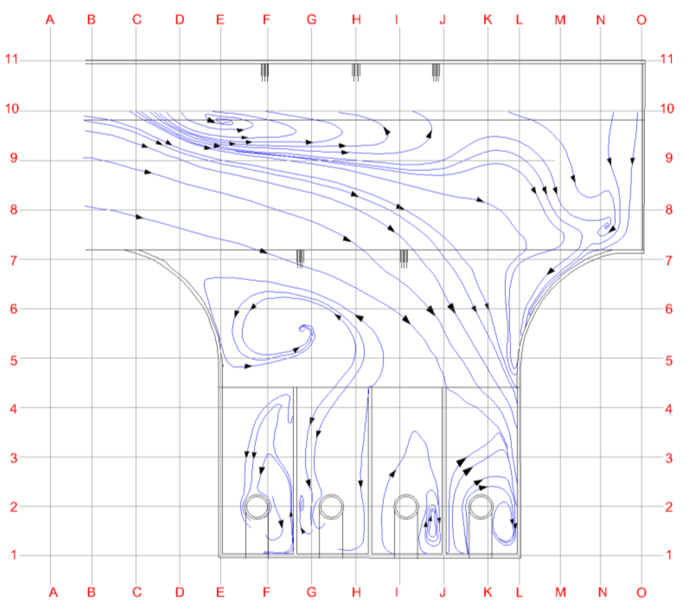
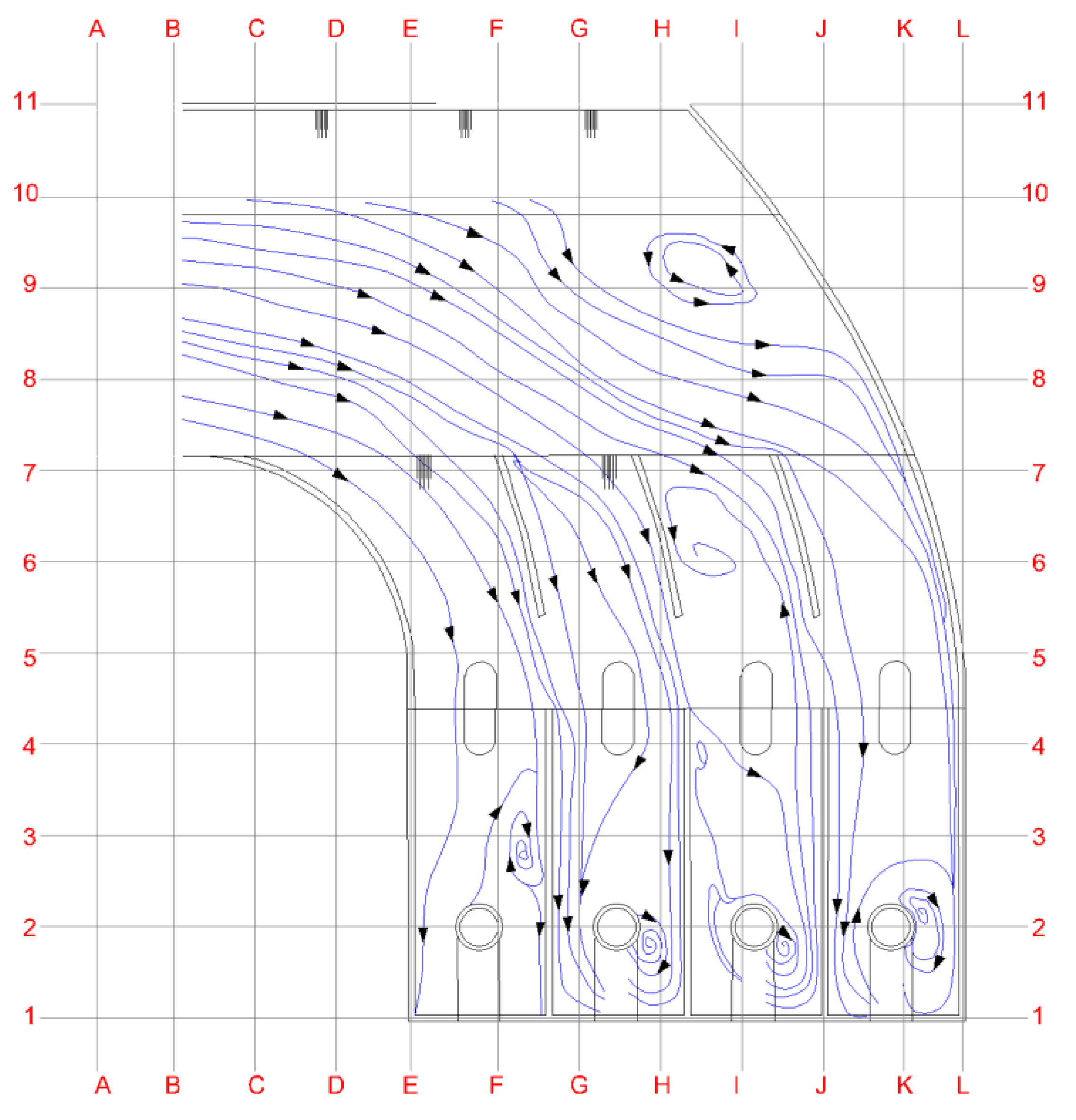
This comparative study started by describing the flow pattern of a subsurface layer 0.95 m from the surface. The flow pattern is discussed for the original case first, then is followed by the five proposed models. The type of vortices is a surface whirlpool, and the area of the vortices is defined as the area around the outermost streamline of swirling flow. As presented in Figure 5, the original case flow pattern shows that a deflection of the stream exit to the pumping station started at section B. The streamlines go towards the right pumping station pool, while backflows generate several vortices. A vortex at sections D-10 appears due to the backflow generated downstream. Another vortex at sections F-5 is caused due to the suction of the two-left pumping station pools and the backflow produced beside the left wall of the pool. Each pumping station pool contains a small vortex beside the suction of the pump. In the first right pool, a vortex appears near sections K-2, and in the second right pool, another whirl is produced due to the pump suction near area J-2. These two vortexes appeared at the right side of the pump’s suction according to the backflows producing the previously discussed vortex at sections F-5. The vortices in the third and fourth pools from the right were located at the left side of the pump’s suction. The vortex in the third pool from the right appears near sections G-2, and for the fourth pool from the right, it seems close to sections F-2. The wall at section O forms a backflow. If it is modified, it can affect the vortex near cells D-10. This is explored in this study by adding parabolic piers to influence the water velocity and vortices.
The first proposed model viewed in Figure 6 shows the effect of using a parabolic pier downstream. The primary vortex that appeared in the original case transferred from sections D-10 to sections I-9. The vortex that appeared previously in sections F-5 transferred to sections G-5. We can conclude that the parabolic pier downstream transmits these vortices horizontally, even slightly in the four whirlpools in the pumping pools, but they remain in the pools. The two right pools contain vortices above the pump’s suction at sections K-4 and J-3, respectively, while in the two right pools, the eddies seem to be at the center of the pump’s suction. Extending the pool walls in an illustrative manner to parallel the downstream parabolic pier affects the two primary vortices in the original case at sections G-5 and I-9, respectively. However, many small vortices appeared inside the pools, as shown in Figure 7 in the second proposed model.
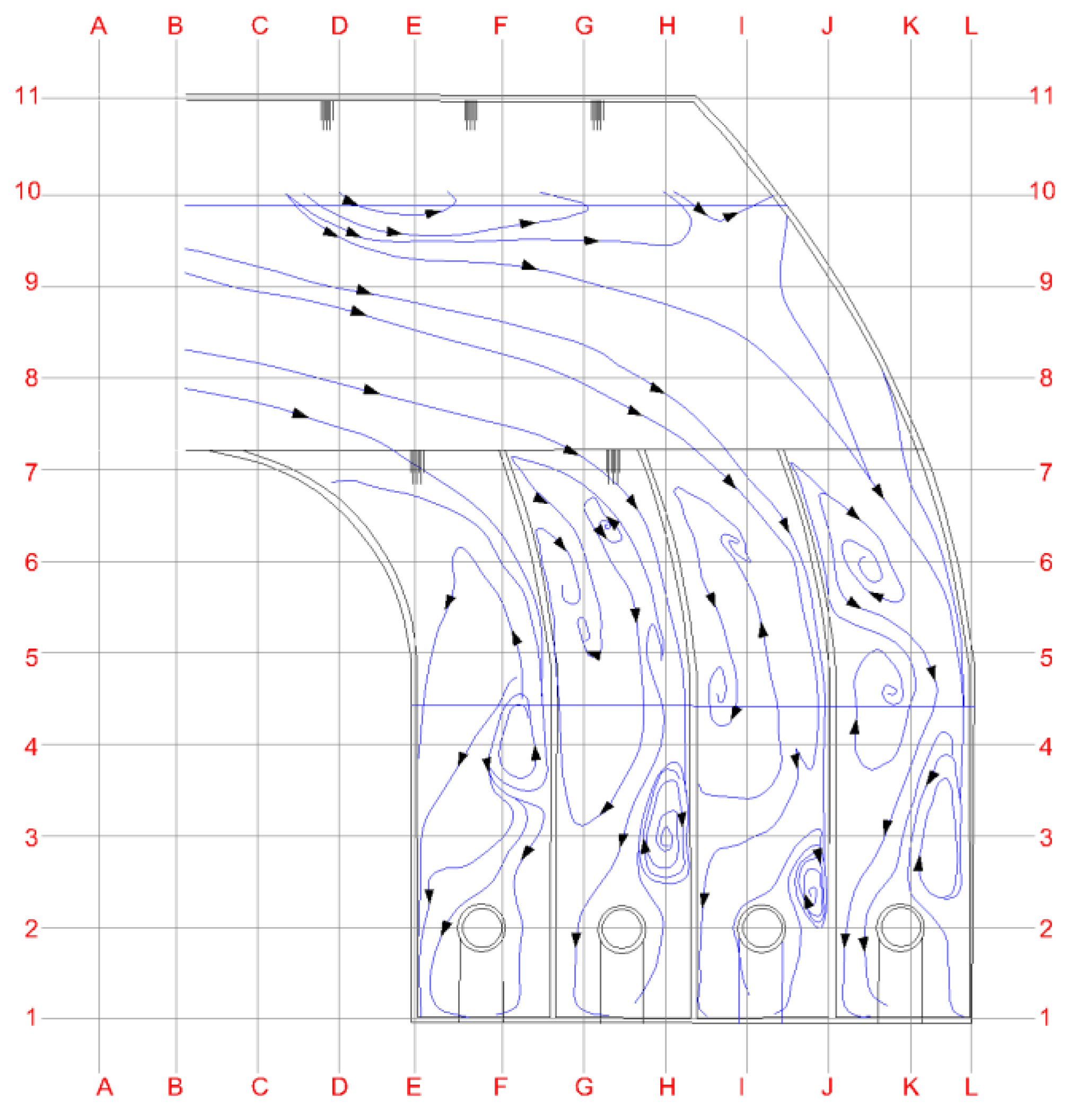
By studying the effect of the separation of the partitions of the parabolic pool in the third proposed model, the number of small vortices increased, as shown in Figure 8. These vortices took place due to backflow as a result of using partitions that the streamlines collided with, and this appeared by analyzing the flow patterns. It was found that most of the vortices are located between Section 4 and Section 6. This concludes that the presence of an obstacle at this range may release these vortices, and it will act as a throttle in which the velocity will also be increased. This leads to the fourth proposed model and the optimum case in this study. While eliminating a large number of vortices, the study may also lead to using a linear submerged pier at the bottom of the upstream to dissipate the presence of the vortices at the bottom; this can be seen in the fifth proposed model.
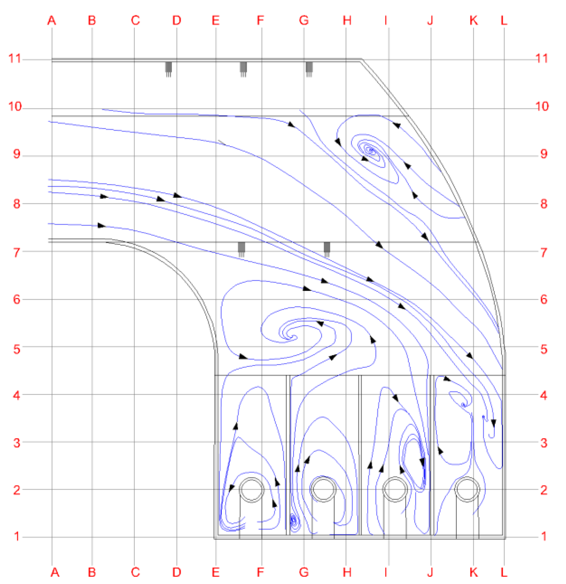
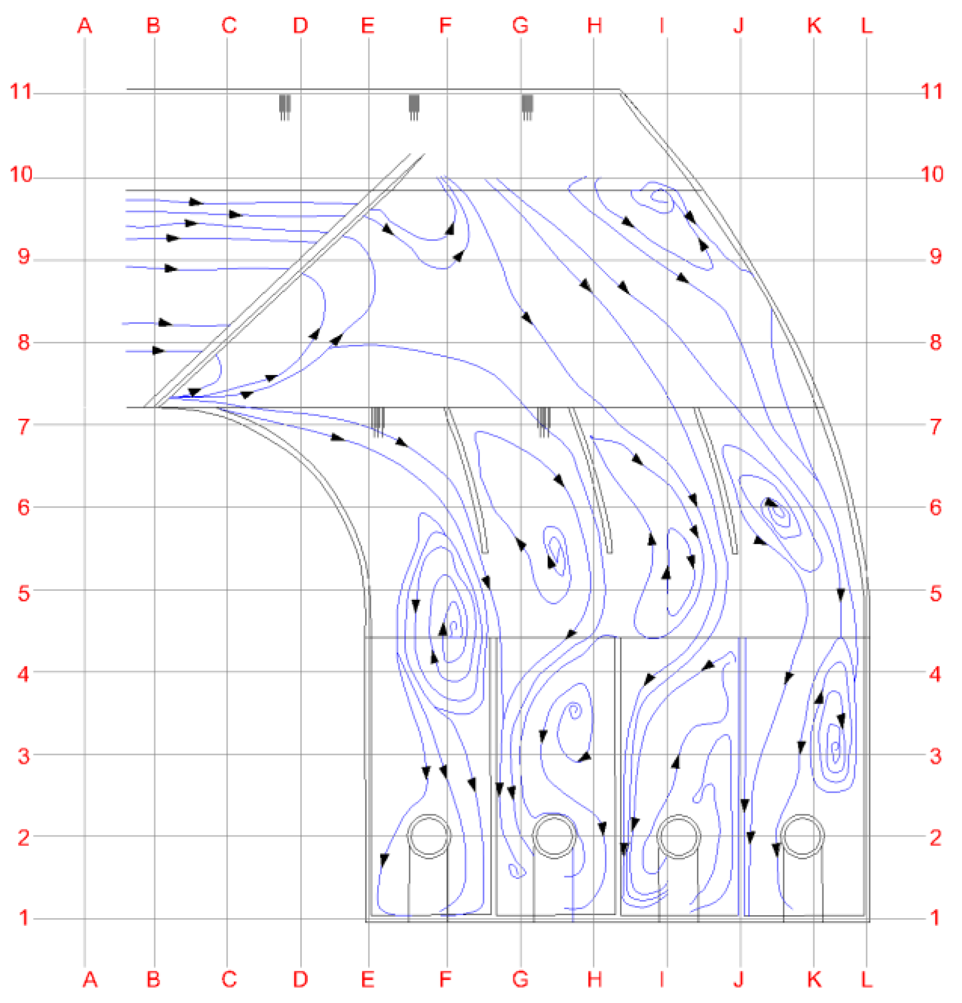
The fourth proposed model appears in Figure 9. It can be concluded that a small vortex near sections H-9 appeared instead of the two whirlpools that appeared in the original case at sections D-9 and E-5. Thus, four small vortices were created, where each one is very close to the pump’s suction in each pool. This resulted from the presence of the four obstacles, which dissipated in the vortices that appeared in the third model and the openings in the pool partition guides.
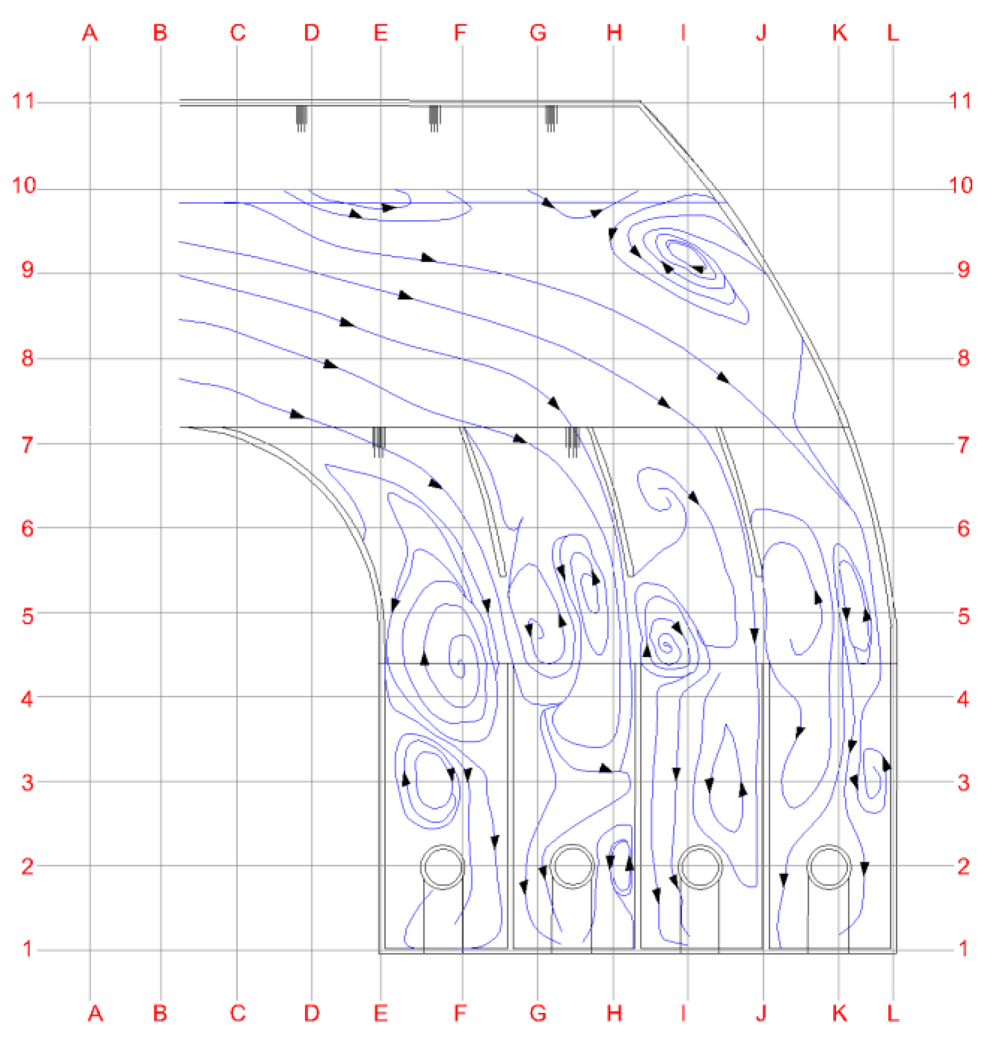
Using the submerged pier shown in the fifth proposed model did not have a significant effect like the fourth model, as shown in Figure 10. It reduced the number of vortices but not by adding obstacles, such as in the fourth proposed model. In this model, eight vortices appeared in the four pools, where each pumping station pool contained two whirlpools. One was above the suction pump and the other near the suction. Eddies above the suction pump appeared due to backflows, while the submerged pier made the small vortices in the third proposed model combine into one vortex above each section pump.
3.2. Flow Velocity Distribution Comparison
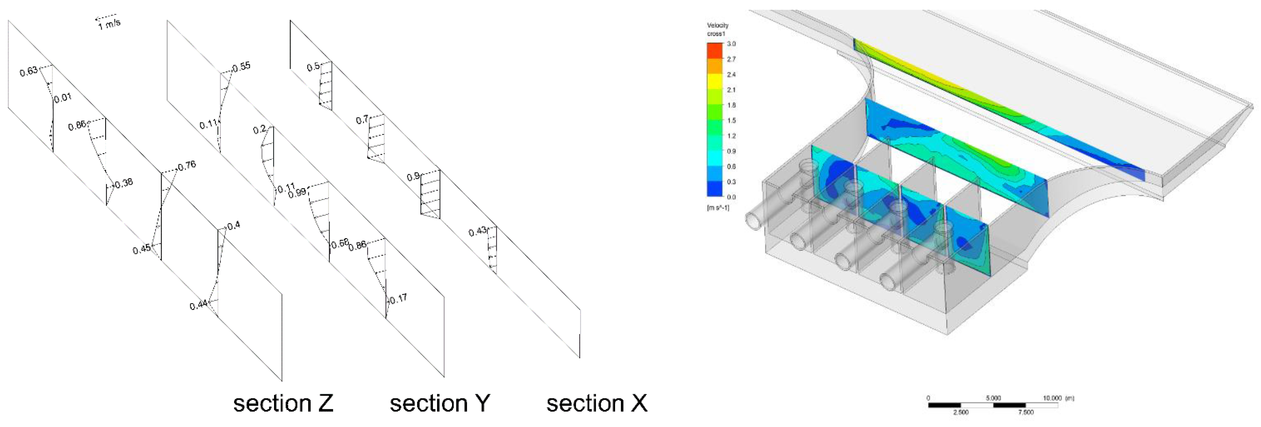
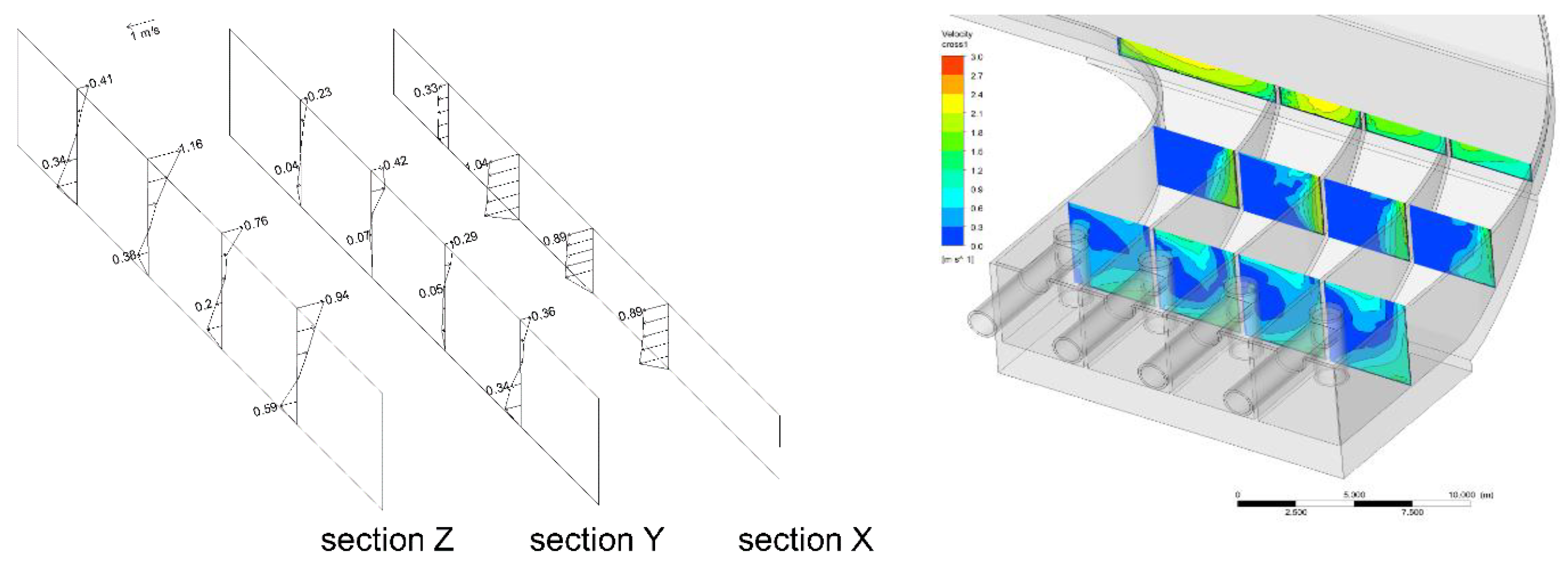
For the velocity distribution shown for the original case, the main flow is biased to the right. The right side of pools shows that flow rate is generally larger than on the left side, and the flow rate from the surface layer to the bottom is gradually reduced. The velocity contours give a significant indication to this bias. This phenomenon appears to be due to backflows, which appeared in section Z in Figure 11. Note that for the shown velocity distributions analysis, section X, Y, and Z are ordered for the velocity distributions shown at the right in Figure 11, Figure 12, Figure 13, Figure 14, Figure 15 and Figure 16. Section X is the farthest from the pumps, while section Z is close to the pumps, and section Y is in between.
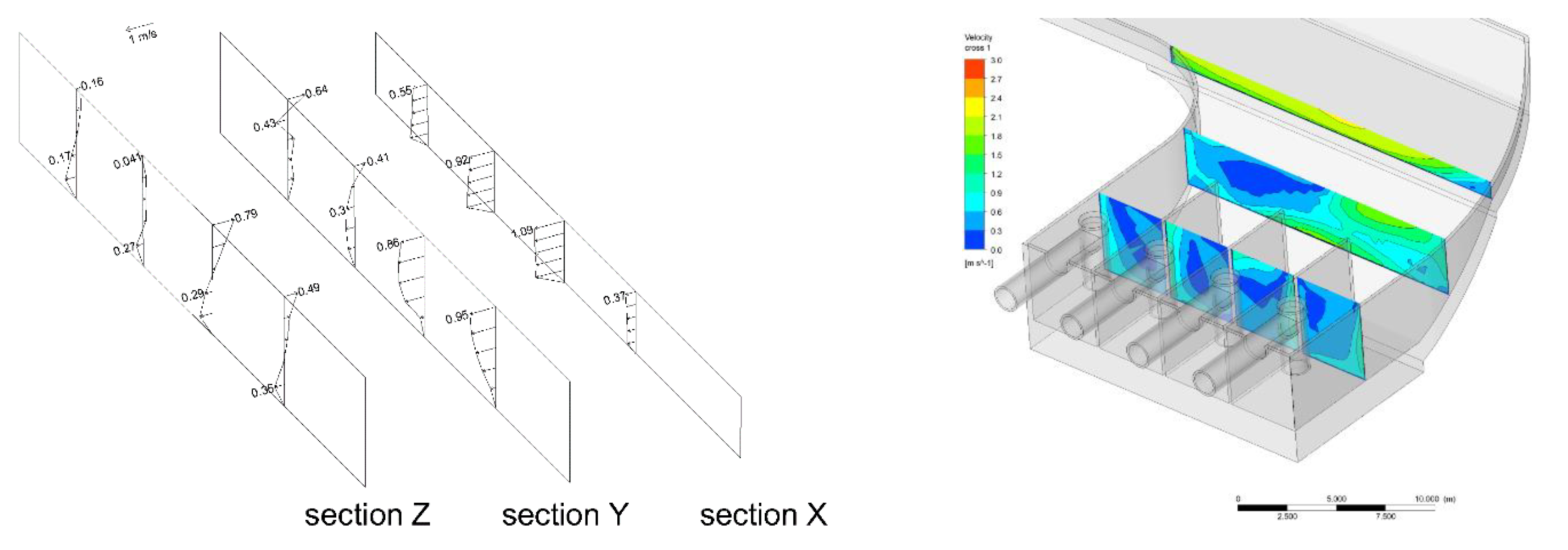
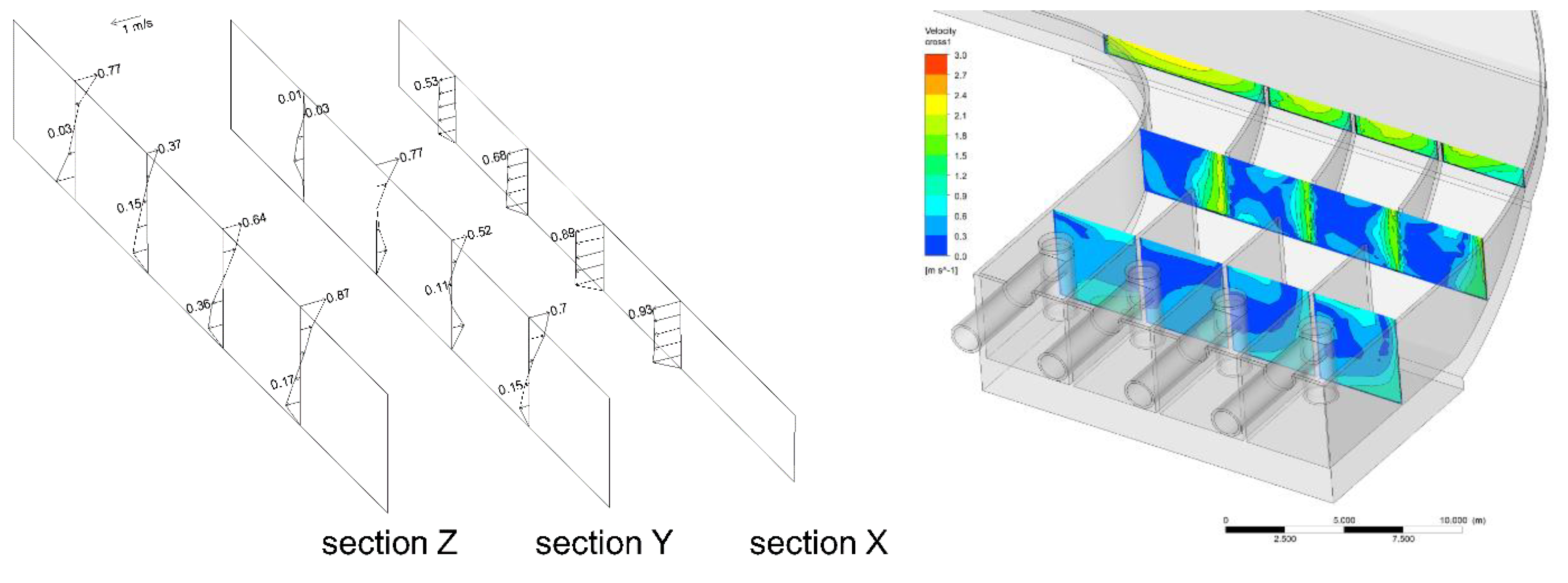
After editing the original case with the parabolic downstream pier, it can be found that the overall water velocity at section Y decreased and the backflows at section Y reduced from the bottom and raised near to the surface. However, backflows still took place in section Z, generating vortices near the suction pumps. This can be noticed clearly in Figure 12.
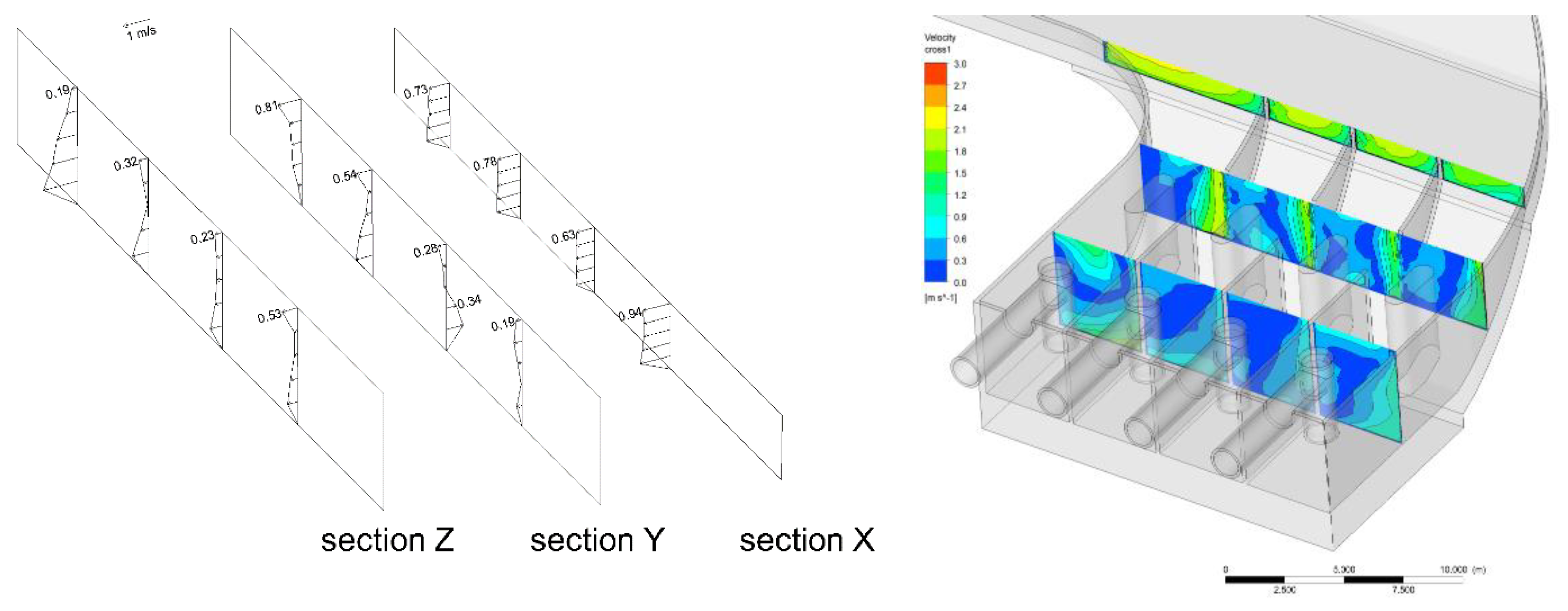
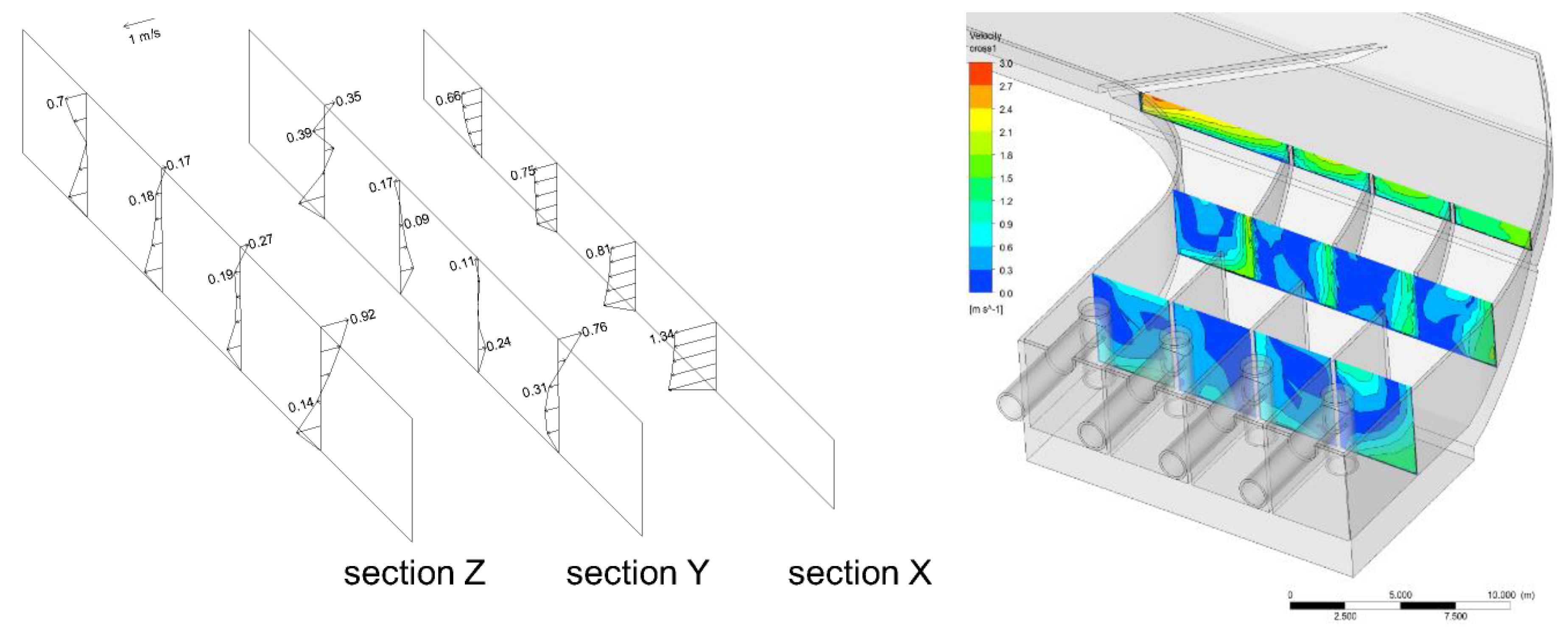
By extending the pool’s partitions in the second proposed model, the overall velocity distribution at section Y reduced by high backflows, generating many vortices inside the pump section pools. According to the comparison of Figure 13 and Figure 14 of the original case to Figure 11, it can be concluded that extending the partitions increases the vortex and also the backflows. However, the overall velocity decreased by allowing an opening in the partitions, such as in the third proposed model, in which the number of vortices was increased. If this is compared to the fourth proposed model in which obstacles were added, this indicates that the dissipation of the vortices reduced the backflows, as shown in Figure 15. Overall, no significant effect of the submerged pier in the fifth proposed model, as in the fourth proposed model, was apparent.
3.3. Uniformity Velocity Distribution of Pump’s Inlet Estimation
To calculate velocity distribution uniformity, the following formula should be used:
where is the axial velocity of the ith grid unit, m/s; is the average axial flow rate in the pump’s inlet, m/s; The area of the ith grid unit m2; n is the total number of grid cells in the overflow section.
The parabolic piers and obstacles increase the velocity across the pumps. The speed of the water at the inlet of the pump is the maximum at the fourth proposed model. This can be expressed through Table 3.
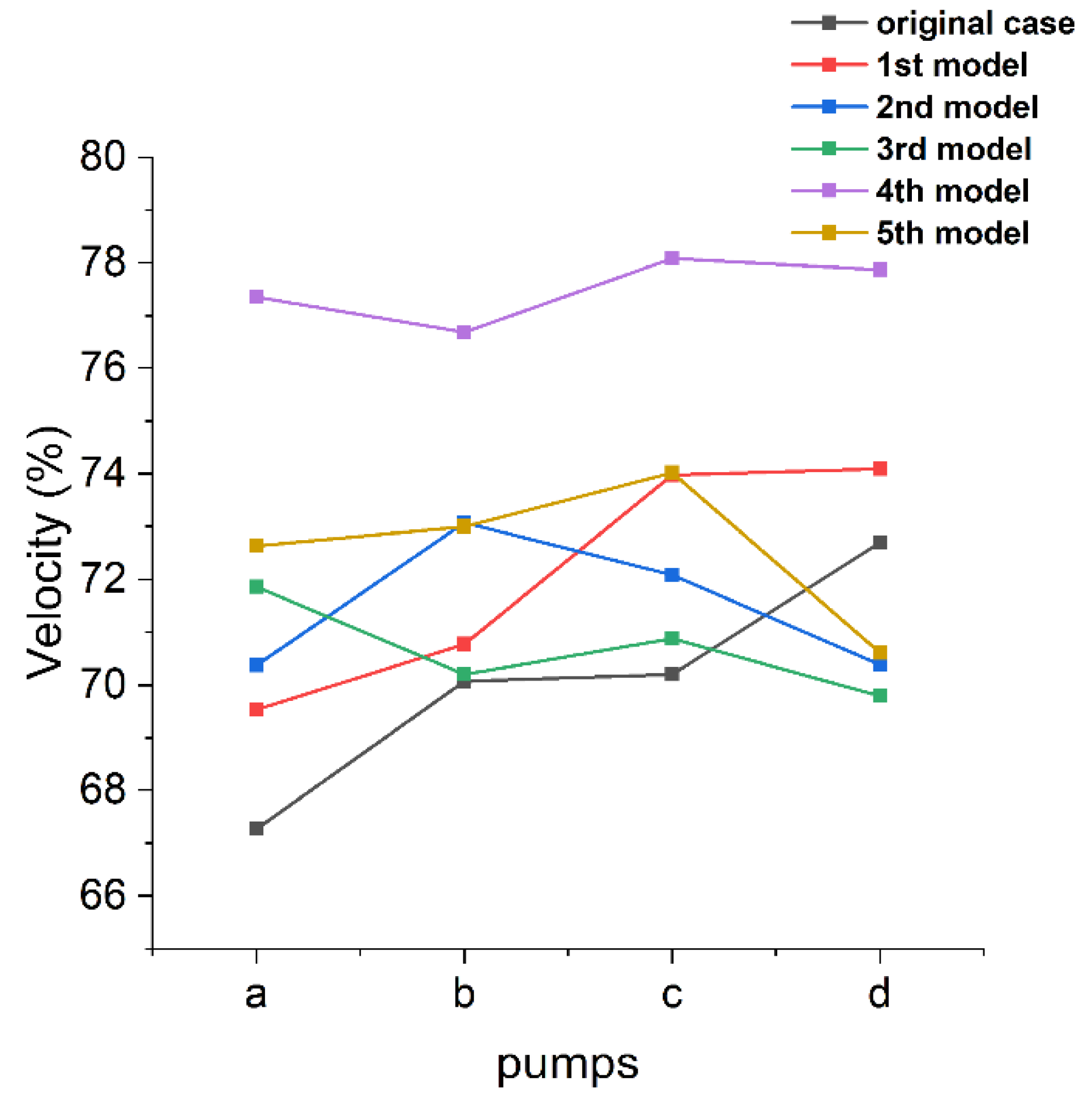
The vortices generated affect the velocity of water directly at the pump’s inlet. According to Figure 17, the original case at the pump (a) had the lowest inlet velocity while the pump (d) showed the maximum. This is due to the deflection of the stream towards the pumping pools. The study was conducted to make the deflection effect uniform and increase the speed at the pump’s inlet. By adding the parabolic downstream pier in the first proposed model, the curve pattern seemed to be the same as the original case. From this point of view, the lowest point was at the pump (a) and the highest one was at the pump (d). At the second proposed model, the curve pattern was changed to be the maximum velocity achieved at the pump (b), while the lowest was still at pump (a). The third proposed model for overall pump speed seemed to be less than the second, but pump (a) was still the lowest velocity value. Finally, the optimum appeared in the fourth proposed model in which pump (a) achieved the maximum velocity value against all the patterns of all studied cases. The uniformity reached a better value in the fifth proposed model for pumps (a), (b), and (c) but pump (d) exhibited the lowest value. For the fourth proposed model, it reached the highest velocities at each pump and the deflection of the streamlines was modified to make pump (a) reach the maximum velocity value.
3.4. Vortex Reduction Estimation
In order to quantify the influence of rectification measures on eddy suppression under the design operating conditions, the parameter ratio of the eddy area and the reduction rate of the eddy area were introduced. The eddy areas of the original case and five proposed models were compared. The vortices reduction rates were computed according to these formulas [45]:
where is the reduction rate of the eddy area , is the vortex area and is the forebay area .
From the gained results of the vortices reduction rate, it was found that the best case was the fourth proposed model, in which the calculated rate reached 70.56%. While the second proposed model reached 29.737% without obstacles and the extension of the parabolic partitions, the lowest case was the fifth one with the submerged block which reached 14.477%. These results can be considered a confirmation of the previously discussed flow pattern analysis as shown in Table 4.
To study the effect of proposed models, the vortex reduction was calculated near the suction of the pump station. It was noticed that the best model to accomplish a minimum vortex area was the fourth proposed model, with an area 11.352 and a reduction rate of 80.67%, as shown in Table 5.
4. Conclusions
The flow pattern of a pumping station can be improved to enhance pump performance, minimize sedimentation, improve the pumping station’s reliability and economy, lower expenses, and increase efficiency. In this research, a case study and five proposed models were established by SOLIDWORKS modeling software and analyzed by ANSYS-CFX. Many rectification measures have been explored opposite the pump station to progress the flow pattern, including all proposed models in this paper. Mesh independence, the convergence of the grid, uniformity velocity distribution of pumps, and vortex reduction were estimated from the numerical simulation. Compared to the numerical simulation results, choosing the best scheme can ameliorate the flow pattern and reduce the whirlpools.
- In the original case, as shown in Figure 1, the flow pattern in the forebay is complicated and has a large vortex area, which has a terrible effect on the safety of the operating of the pump station.
- In the fourth proposed model, as shown in Figure 2d, the flow pattern improved. The reduction rate of the vortex decreased by 70%. The velocity uniformity is also better than it was in the original plan.
- The fifth proposed model, as shown in Figure 2e, proves that adding submerged obstacles is not an optimal solution for this case study.
- In Figure 5, Figure 6, Figure 7, Figure 8, Figure 9 and Figure 10, the most critical zone for the pump water intake is between 0 to 5 lines E and L in the grid, which define the water intake behavior. The objective of the study was to eliminate the vortices as much as possible. These vortices affect the behavior of the pump, while the flow behavior is described in Section 3.1 with the flow pattern comparison.
Author Contributions
Conceptualization, F.Y.; software and writing—original draft preparation, A.N.; writing—review and editing, F.Y. and M.H.; Investigation, Y.Z. and T.W.; supervision, F.Y. All authors have read and agreed to the published version of the manuscript.
Funding
This research was funded by the National Natural Science Foundation of China (grant No. 51609210), major projects of the Natural Science Foundation of the Jiangsu Higher Education Institutions of China (grant No. 20KJA570001), the open research subject of the Key Laboratory of Fluid and Power Machinery, Ministry of Education (szjj2016-078), the Science and Technology Plan Project of the Yangzhou City (grant No. YZU201901), the Technology Project of the Water Resources Department of the Jiangsu Province (grant No. 2020029), and the Priority Academic Program Development of the Jiangsu Higher Education Institutions (PAPD).
Institutional Review Board Statement
Not applicable.
Informed Consent Statement
Not applicable.
Data Availability Statement
All data necessary to carry out the work in this paper are included in the figures, tables or are available in the cited references.
Conflicts of Interest
The authors declare that they have no conflict of interest.
References
- Song, W.; Pang, Y.; Shi, X.; Xu, Q. Study on the Rectification of Forebay in Pumping Station. Math. Probl. Eng. 2018, 2018, 2876980. [Google Scholar] [CrossRef]
- Kong, J.; Skjelbred, H.I.; Fosso, O.B. An overview on formulations and optimization methods for the unit-based short-term hydro scheduling problem. Electr. Power Syst. Res. 2020, 178, 106027. [Google Scholar] [CrossRef]
- Caishui, H. Three-dimensional numerical analysis of flow pattern in pressure forebay of hydropower station. Procedia Eng. 2012, 28, 128–135. [Google Scholar] [CrossRef]
- Cheng, B.; Yu, Y. CFD simulation and optimization for lateral diversion and intake pumping stations. Procedia Eng. 2012, 28, 122–127. [Google Scholar] [CrossRef] [Green Version]
- Jiangang, F.; Xiaosheng, W.; Bin, C. Experimental Study on the Flow Pattern Modifying in the Fore Bay of large Urban Side Inflow Pumping Stations. Procedia Eng. 2012, 28, 214–219. [Google Scholar] [CrossRef] [Green Version]
- Rajendran, V.; Constantinescu, S.; Patel, V. Experimental validation of numerical model of flow in pump-intake bays. J. Hydraul. Eng. 1999, 125, 1119–1125. [Google Scholar] [CrossRef]
- Zhao, H.; Yang, F.; Liu, C.; Chen, S.; He, J. Numerical simulation of side-intake flow for fluid meliorating of pumping stations. Water Resour. Hydropower Eng. 2017, 48, 79–84. [Google Scholar]
- Can, L.; Chao, L. Numerical simulation and improvement of side-intake characteristics of multi-unit pumping station. J. Hydroelectr. Eng. 2015, 34, 207–214. [Google Scholar]
- Zhou, J.; Zhong, Z.; Liang, J.; Shi, X. Three-dimensional Numerical Simulation of Side-intake Forebay of Pumping Station. J. Irrig. Drain. 2015, 34, 52–55. [Google Scholar]
- Xia, C.; Cheng, L.; Zhao, G.; Yu, L.; Wu, M.; Xu, W. Numerical simulation of flow pattern in forebay of pump station with single row of square columns. Adv. Sci. Technol. Water Resour. 2017, 37, 53–58. [Google Scholar]
- Zhang, Y.L.; Song, S.L.; Chen, Y.; Liu, X.; Fu, X.-Q. Numerical Simulation of Rectification Measures for Side-direction Forebay in Pump Station. China Rural Water Hydropower 2016, 5, 117–120. [Google Scholar]
- Ansar, M.; Nakato, T.; Constantinescu, G. Numerical simulations of inviscid three-dimensional flows at single-and dual-pump intakes. J. Hydraul. Res. 2002, 40, 461–470. [Google Scholar] [CrossRef]
- Yonghai, Y.; Bin, C. CFD simulation and optimization on inflow pattern of diversion and intake pumping stations with side-inlets. Water Resour. Hydropower Eng. 2012, 43, 72–75. [Google Scholar]
- Chen, H.-X.; Guo, J.-H. Numerical simulation of 3-D turbulent flow in the multi-intakes sump of the pump station. J. Hydrodyn. 2007, 19, 42–47. [Google Scholar] [CrossRef]
- Das, A. Optimal design of channel having horizontal bottom and parabolic sides. J. Irrig. Drain. Eng. 2007, 133, 192–197. [Google Scholar] [CrossRef]
- Borenäs, K.; Lundberg, P. Rotating hydraulics of flow in a parabolic channel. J. Fluid Mech. 1986, 167, 309–326. [Google Scholar] [CrossRef]
- Abdelmeguid, A.M.; Markatos, N.C.; Muraoka, K.; Spalding, D.B. A comparison between the parabolic and partially-parabolic solution procedures for three-dimensional turbulent flows around ships’ hulls. Appl. Math. Model. 1979, 3, 249–258. [Google Scholar] [CrossRef]
- Easa, S.M. Improved channel cross section with two-segment parabolic sides and horizontal bottom. J. Irrig. Drain. Eng. 2009, 135, 357–365. [Google Scholar] [CrossRef]
- Vatankhah, A.R. Water surface profile along a side weir in a parabolic channel. Flow Meas. Instrum. 2013, 32, 90–95. [Google Scholar] [CrossRef]
- Banchetti, J.; Luchini, P.; Quadrio, M. Turbulent drag reduction over curved walls. J. Fluid Mech. 2020, 896, A10. [Google Scholar] [CrossRef]
- Biswas, A.; Raman, A.K.; Mullick, A. A Numerical Simulation of Turbulent Flow through a Curved Duct. Mapana J. Sci. 2012, 11, 169–178. [Google Scholar] [CrossRef]
- Chahar, B.R. Optimal design of parabolic canal section. J. Irrig. Drain. Eng. 2005, 131, 546–554. [Google Scholar] [CrossRef] [Green Version]
- Chen, Y.L.; Hung, J.B.; Hsu, S.L.; Hsiao, S.C.; Wu, Y.C. Interaction of water waves and a submerged parabolic obstacle in the presence of a following uniform/shear current using RANS model. Math. Probl. Eng. 2014, 2014, 896723. [Google Scholar] [CrossRef] [Green Version]
- Yanuka, D.; Shafer, D.; Krasik, Y. Shock wave convergence in water with parabolic wall boundaries. J. Appl. Phys. 2015, 117, 163305. [Google Scholar] [CrossRef] [Green Version]
- Bautista, E.G.; Méndez, F.; Bautista, O.; Mora, A. Propagation of shallow water waves in an open parabolic channel using the WKB perturbation technique. Appl. Ocean Res. 2011, 33, 186–192. [Google Scholar] [CrossRef]
- Domfeh, M.K.; Gyamfi, S.; Amo-Boateng, M.; Andoh, R.; Ofosu, E.A.; Tabor, G. Free surface vortices at hydropower intakes: A state-of-the-art review. Sci. Afr. 2020, 8, e00355. [Google Scholar] [CrossRef]
- Liu, C.; Zhou, J.; Cheng, L. The Experimental Study and Numerical Simulation of Turbulent Flow in Pumping Forebay. ASME Power Conf. 2009, 43505, 171–176. [Google Scholar]
- Li, X.; Zheng, Y. Numerical simulation and hydraulic optimization of the lateral oblique forebay. In Proceedings of the 2011 International Conference on Remote Sensing, Environment and Transportation Engineering, Nanjing, China, 24–26 June 2011. [Google Scholar]
- Eslamdoost, A.; Vikström, M. A body-force model for waterjet pump simulation. Appl. Ocean Res. 2019, 90, 101832. [Google Scholar] [CrossRef]
- Ansar, M.; Nakato, T. Experimental study of 3D pump-intake flows with and without cross flow. J. Hydraul. Eng. 2001, 127, 825–834. [Google Scholar] [CrossRef]
- Zheng, Y.; Werth, D. Optimize pump intake design with formed suction inlets. In Proceedings of the World Environmental and Water Resources Congress, Honolulu, HI, USA, 12–16 May 2008. [Google Scholar]
- Jun, L.; Yongmei, C.; Chuanchang, G. Numerical simulation of flow patterns in the forebay and suction sump of tianshan pumping station. Water Pract. Technol. 2014, 9, 519–525. [Google Scholar]
- Olimstad, G.; Østby, P.T.K. Failure and redesign of a high-speed pump with respect to rotor-stator interaction. Eng. Fail. Anal. 2019, 104, 704–713. [Google Scholar] [CrossRef]
- Qian, Z.; Wang, Y.; Huai, W.; Lee, Y. Numerical simulation of water flow in an axial flow pump with adjustable guide vanes. J. Mech. Sci. Technol. 2010, 24, 971–976. [Google Scholar] [CrossRef]
- Chen, Y.L.; Wu, C.; Ye, M.; Ju, X.M. Hydraulic characteristics of vertical vortex at hydraulic intakes. J. Hydrodyn. 2007, 19, 143–149. [Google Scholar] [CrossRef]
- Nagahara, T.; Sato, T.; Okamura, T.; Iwano, R. Measurement of the Flow around the Submerged Vortex Cavitation in a Pump Intake by Means of PIV. In Proceedings of the Fifth International Symposium on Cavitation, Osaka, Japan, 1–4 November 2003. [Google Scholar]
- Rajendran, V.; Patel, V. Measurement of vortices in model pump-intake bay by PIV. J. Hydraul. Eng. 2000, 126, 322–334. [Google Scholar] [CrossRef]
- Shabayek, S.A. Improving approach flow hydraulics at pump intakes. Int. J. Civ. Environ. Eng. 2010, 10, 23–31. [Google Scholar]
- Liu, C.; Zhou, J.; Cheng, L.; Jin, Y.; Han, X. Study on Improving the Flow in Forebay of the Pumping Station. In Proceedings of the Fluids Engineering Division Summer Meeting, Montreal, QC, Canada, 1–5 August 2010. [Google Scholar]
- Roache, P.J. Quantification of uncertainty in computational fluid dynamics. Annu. Rev. Fluid Mech. 1997, 29, 123–160. [Google Scholar] [CrossRef] [Green Version]
- Savage, B.M.; Crookston, B.M.; Paxson, G.S. Physical and numerical modeling of large headwater ratios for a 15 labyrinth spillway. J. Hydraul. Eng. 2016, 142, 04016046. [Google Scholar] [CrossRef]
- Liu, H.; Liu, M.; Bai, Y.; Du, H.; Dong, L. Grid convergence based on GCI for centrifugal pump. J. Jiangsu Univ. Nat. Sci. Ed. 2014, 35, 279–283. [Google Scholar]
- Wang, S.S.; Roache, P.J.; Schmalz, R.A.; Jia, Y.; Smith, P.E. Verification and Validation of 3D Free-Surface Flow Models; American Society of Civil Engineers: Reston, VA, USA, 2008. [Google Scholar]
- Yabing, D. Numerical Simulation Study on the Scheme of Trajecmtory Bucket Type Energy Dissipation for Overflow Sam of Shiziya Reservoir; Xi’an University of Technology: Xi’an, China, 2018. [Google Scholar]
- Yang, F.; Zhang, Y.; Liu, C.; Wang, T.; Jiang, D.; Jin, Y. Numerical and Experimental Investigations of Flow Pattern and Anti-Vortex Measures of Forebay in a Multi-Unit Pumping Station. Water 2021, 13, 935. [Google Scholar] [CrossRef]
Figure 1.
Overall layout view of the original case (in meters).

Figure 2.
Different proposed models.

Figure 3.
Plans to compute the head loss.

Figure 4.
Computed head loss chart at different grid numbers.

Figure 5.
Streamline distribution for the original case.

Figure 6.
Streamline distribution for the first proposed model.

Figure 7.
Streamline distribution for the second proposed model.

Figure 8.
Streamline distribution for the third proposed model.

Figure 9.
Streamline distribution for the fourth proposed model.

Figure 10.
Streamline distribution for the fifth proposed model.

Figure 11.
Analysis and numerical simulation for flow velocity distribution for the original case.

Figure 12.
Analysis and numerical simulation for flow velocity distribution for the first proposed model.
Figure 12.
Analysis and numerical simulation for flow velocity distribution for the first proposed model.

Figure 13.
Analysis and numerical simulation for flow velocity distribution for the second proposed model.
Figure 13.
Analysis and numerical simulation for flow velocity distribution for the second proposed model.

Figure 14.
Analysis and numerical simulation for flow velocity distribution for the third proposed model.
Figure 14.
Analysis and numerical simulation for flow velocity distribution for the third proposed model.

Figure 15.
Analysis and numerical simulation for flow velocity distribution for the fourth proposed model.
Figure 15.
Analysis and numerical simulation for flow velocity distribution for the fourth proposed model.

Figure 16.
Analysis and numerical simulation for flow velocity distribution for the fifth proposed model.
Figure 16.
Analysis and numerical simulation for flow velocity distribution for the fifth proposed model.

Figure 17.
Velocity distribution at pump’s inlet.


Table 1.
Head loss under different grid numbers.
| No. Grids | 1,150,115 | 2,093,038 | 3,067,875 | 4,186,264 | 5,016,607 | 6,096,321 |
|---|---|---|---|---|---|---|
| head loss (m) | 0.110 | 0.120 | 0.130 | 0.133 | 0.137 | 0.137 |
Table 2.
GCI calculation result.
| Total Number of Grid Points | r(Dk/Dk+1) | P | Q m3/s | ||
|---|---|---|---|---|---|
| 1,150,115 | 17 | ||||
| 2,093,038 | 1.82 | 1 | 17.23 | 0.01335 | 2.03525 |
| 3,067,875 | 1.47 | 1 | 17.19 | 0.00233 | 0.62451 |
| 4,186,264 | 1.36 | 1 | 17.15 | 0.00233 | 0.79974 |
| 5,016,607 | 1.20 | 1 | 17.13 | 0.00117 | 0.73579 |
| 6,096,321 | 1.22 | 1 | 17.12 | 0.00058 | 0.33924 |
Table 3.
Velocity Distribution at the Pumps inlet (pump ordered a, b, c, and d from the right to the left).
Table 3.
Velocity Distribution at the Pumps inlet (pump ordered a, b, c, and d from the right to the left).
| Cases | Velocity Distribution at the Pumps Inlet (%) | |||
|---|---|---|---|---|
| (a) | (b) | (c) | (d) | |
| Original case | 65.27 | 70.07 | 70.20 | 71.70 |
| First proposed model | 69.53 | 70.78 | 73.98 | 74.09 |
| Second proposed model | 70.37 | 73.07 | 72.08 | 70.39 |
| Third proposed model | 71.86 | 70.21 | 70.88 | 69.79 |
| fourth proposed model | 77.35 | 76.68 | 78.08 | 77.87 |
| Fifth proposed model | 72.63 | 73.00 | 74.03 | 70.61 |
Table 4.
Vortex reduction estimation for the whole forebay.
| Plan Number | Vortex Area m2 | Forebay Area m2 | Area Ratio % | Reduction Rate % |
|---|---|---|---|---|
| Original Case | 86.281 | 690.186 | 12.501 | - |
| First Proposed Model | 50.436 | 574.201 | 8.784 | 29.737 |
| Second Proposed Model | 51.500 | 574.201 | 8.969 | 28.255 |
| Third Proposed Model | 49.644 | 574.201 | 8.646 | 30.840 |
| Fourth Proposed Model | 22.086 | 574.201 | 3.846 | 70.56 |
| Fifth Proposed Model | 61.389 | 574.201 | 10.691 | 14.477 |
Table 5.
Vortex reduction estimation in front of the pump station (lines E–L and 1–5).
| Plan Number | Vortex Area m2 | In Front Pool Area m2 | Area Ratio % | Reduction Rate % |
|---|---|---|---|---|
| Original Case | 58.721 | 252.457 | 23.260 | - |
| First Proposed Model | 35.452 | 252.457 | 14.043 | 39.626 |
| Second Proposed Model | 37.963 | 252.457 | 15.037 | 35.350 |
| Third Proposed Model | 27.625 | 252.457 | 10.942 | 52.956 |
| Fourth Proposed Model | 11.351 | 252.457 | 4.496 | 80.670 |
| Fifth Proposed Model | 42.852 | 252.457 | 16.970 | 27.041 |
Publisher’s Note: MDPI stays neutral with regard to jurisdictional claims in published maps and institutional affiliations. |
© 2021 by the authors. Licensee MDPI, Basel, Switzerland. This article is an open access article distributed under the terms and conditions of the Creative Commons Attribution (CC BY) license (https://creativecommons.org/licenses/by/4.0/).
Share and Cite
MDPI and ACS Style
Nasr, A.; Yang, F.; Zhang, Y.; Wang, T.; Hassan, M. Analysis of the Flow Pattern and Flow Rectification Measures of the Side-Intake Forebay in a Multi-Unit Pumping Station. Water 2021, 13, 2025. https://doi.org/10.3390/w13152025
AMA Style
Nasr A, Yang F, Zhang Y, Wang T, Hassan M. Analysis of the Flow Pattern and Flow Rectification Measures of the Side-Intake Forebay in a Multi-Unit Pumping Station. Water. 2021; 13(15):2025. https://doi.org/10.3390/w13152025
Chicago/Turabian StyleNasr, Ahmed, Fan Yang, Yiqi Zhang, Tieli Wang, and Mahmoud Hassan. 2021. "Analysis of the Flow Pattern and Flow Rectification Measures of the Side-Intake Forebay in a Multi-Unit Pumping Station" Water 13, no. 15: 2025. https://doi.org/10.3390/w13152025
Note that from the first issue of 2016, this journal uses article numbers instead of page numbers. See further details here.