
Prediction of Slow-Moving Landslide Mobility Due to Rainfall Using a Two-Wedges Model


Department of Civil Engineering, University of Calabria, 87036 Rende, Italy
*
Author to whom correspondence should be addressed.
Water 2021, 13(15), 2030; https://doi.org/10.3390/w13152030
Submission received: 24 June 2021
/
Revised: 19 July 2021
/
Accepted: 21 July 2021
/
Published: 25 July 2021
(This article belongs to the Special Issue Effects of Water on Slope Stability)
Abstract
:In the present study, the landslides cyclically reactivated by water-table oscillations due to rainfall are dealt with. The principal kind of motion that usually characterizes such landslides is a slide with rather small velocity. As another feature, soil deformations are substantially accumulated inside a narrow shear zone situated below the landslide body so that the latter approximately slides rigidly. Within this framework, a new approach is developed in this paper to predict the mobility of this type of landslides due to rainfall. To this end, a two-wedges model is used to schematize the moving soil mass. Some analytical solutions are derived to link rain recordings with water-table fluctuations and in turn to landslide displacements. A well-documented landslide frequently activated by rainfall is studied to check the forecasting capacity of the proposed method.
1. Introduction
Landslide mobility is often connected to the water-table fluctuations owing to weather, and therefore, it is distinguished by an alternation of stages of movement and inactivity. Particularly, a reactivation of the landslide or an acceleration of the motion (if it is moving) can be caused by a raising in the water table throughout rainy periods. On the other hand, a decreasing in the groundwater table occurring in arid periods causes a lowering of the displacement rate of the unstable soil mass, leading eventually to the stop of the motion. According to the classification system of Cruden and Varnes [1], these landslides are categorized as very slow-moving landslides and are characterized by a displacement rate of approximately a few centimeters per year. A further common characteristic of such landslides is that the soil strains are usually located inside a narrow shear band situated at the base of the unstable soil mass in which the shear strength of the soil is under residual conditions owing to the important gained deformations [2]. Contrarily, the landslide body is subjected to low level of deformation and is generally outlined by horizontal displacements that are substantially steady along the depth. In other words, the unstable soil mass practically slides rigidly.
In engineering practice, the problem is commonly dealt with by separately analyzing the changes in groundwater regime and slope stability by means of an uncoupled approach. In particular, groundwater pressures at the level of the slip surface due to rain infiltration are firstly evaluated, and the latter are afterwards used in a limit equilibrium approach to calculate a slope-safety factor. However, a rational forecasting of the landslide mobility is more useful from a practical point of view than a safety factor calculation, especially when some structures are located on the slope. In these circumstances, the designer should assess whether the calculated displacements exceed the tolerable values established to safeguard the serviceability of the existing structures or prevent their damage [3,4]. Advanced numerical techniques can undeniably accomplish this target, providing a good comprehension of the complicated deformation processes that characterize the slope behaviour [5,6,7,8,9,10,11]. Since the soil viscosity exerts a fundamental role in slow-moving landslides [12,13,14,15,16,17,18], a constitutive model based on the elasto-viscoplastic theory is generally used when performing such a type of simulation [19,20,21,22]. This may sensibly increase the computational costs as well as need many input parameters that are often of difficult experimental evaluation. Therefore, the usage of numerical techniques might not be rational when dealing with routine applications.
Several methods of practical interest were also published in the literature [23,24,25,26,27,28,29,30,31,32,33]. Such methods are generally able to calculate the landslide velocity when groundwater level measurements are available. Therefore, their use is unsuitable for predictive purposes. To overcome this limitation, Conte et al. [34] developed a simple method based on the infinite slope model to relate landslide mobility to rainfall. In this paper, the approach originally introduced by Conte et al. [34] is extended to more complex geometries. Specifically, it is assumed that the unstable soil mass slides on a bi-planar slip surface and can be schematized by means of a two-wedges model. As highlighted by Chowdhury [35], such a schematization may reasonably represent several real situations. Using some analytical solutions derived in this study and rainfall recorded during a sufficiently long time period, the groundwater level fluctuations are evaluated and the landslide velocity predicted. The proposed solution is simple to use and necessitates few data as input, most of which are determined by means of traditional geotechnical tests, whereas the remaining ones are evaluated using a calibration procedure. After this calibration, the method may be adopted to perform a prediction of future displacements of a given landslide body based on weather forecast.
2. Method of Analysis
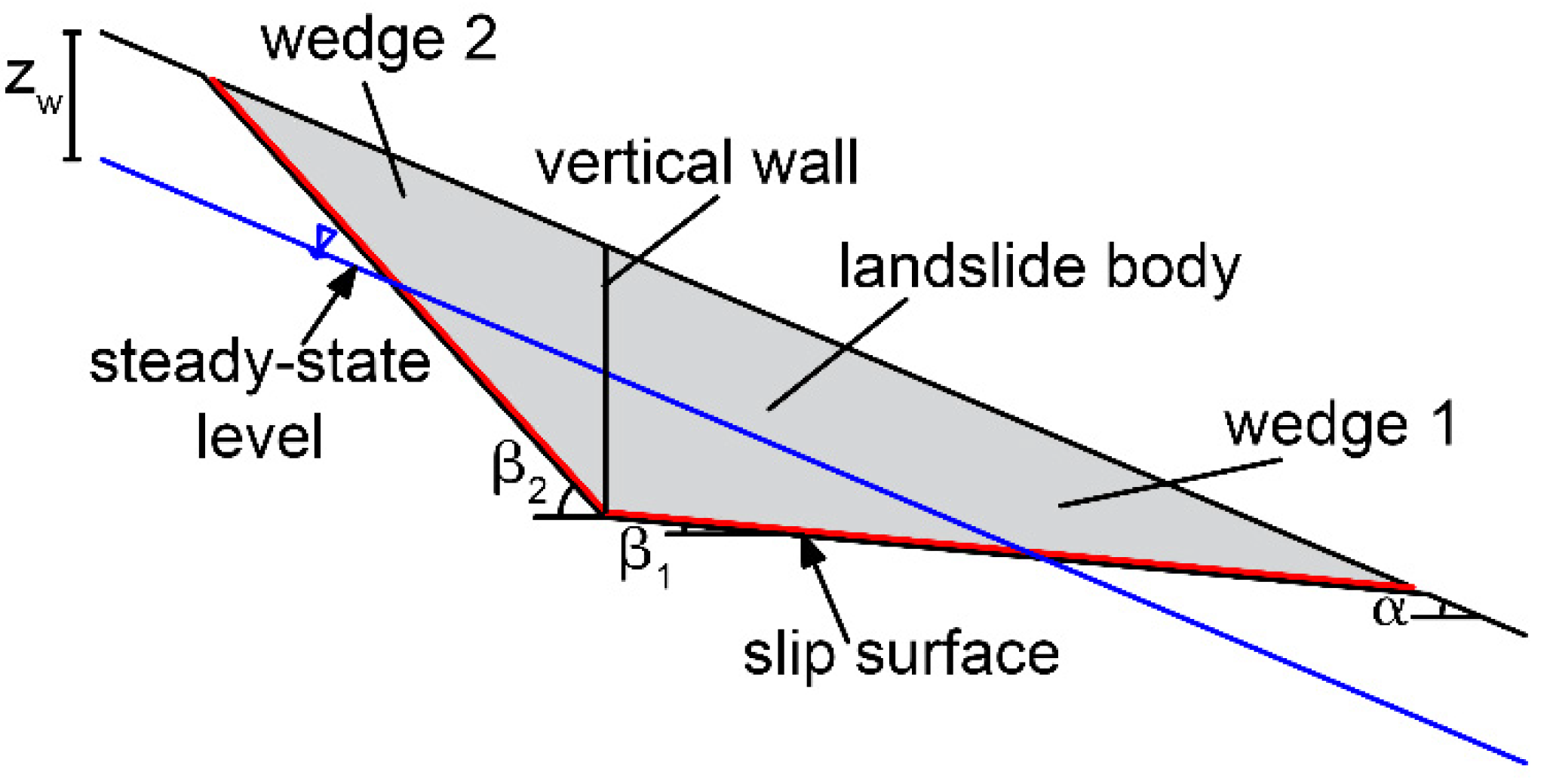
The proposed method uses a two-wedges model to schematize the landslide body. The wedges are separated by an ideal vertical wall and can slide on a bi-planar slip surface, making angles β1 and β2 with the horizontal plane (Figure 1). It is assumed that seepage takes place with flow lines parallel to the slope and a stationary water table located at a depth zw below the ground surface. The water level is subjected to changes h(t) due to rain infiltration.
By assuming that groundwater level oscillates simultaneously with rainfall, h(t) might be calculated as follows [34]:
where ho defines the position of water table at the beginning of the considered period of observation (detected from the stationary position), N is the number of rain events, is a model parameter depending on the soil permeability, where n and Sr are the porosity and the saturation degree of the portion of soil located above the water table, respectively, and hi is the volume of water that can infiltrate in a unity area of the ground surface during the i-th event, whose beginning is defined by toi. Following [36], it is assumed , where p is the potential infiltration rate and represents the maximum water volume that can permeate through a unity area of soil. In the present study, the values of n, Sr, and p are assumed to be constant for the sake of simplicity.
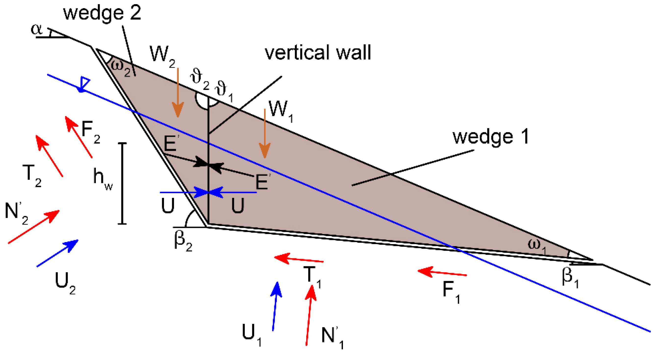
The forces acting on wedge i (with i = 1, 2) are weight Wi along with the forces developed on the failure surface. The latter are the shear force Ti, effective normal force , the force due to water pressure Ui, and the viscous force Fi activated at the base of the unstable soil mass during motion (Figure 2).
Additionally, in correspondence of the vertical interface between the blocks, the resultant of pore water pressure U and the force indicated by act. The latter is inclined of , with respect to the horizontal plane (with , where is the friction angle corresponding to the material forming the landslide body). Forces Wi, U, and Ui can be calculated using the following equations:
and
in which γ is the unit weight of the soil (changes of γ are neglected for the sake of simplicity), Ai represents the volume per unit length of the considered block, hw defines the length of the vertical interface between the two wedges included from the stationary water table to the failure surface, h(t) is provided by Equation (1), and ϑi and ωi are the angles shown in Figure 2. The viscous forces activated at the base of the landslide body during motion are expressed as:
where μs is a coefficient of viscosity of the soil in the shear zone, the expression of which is provided in Appendix A, and vi(t) is the velocity of the i-th block at time t in the movement direction. Forces T1, T2, , , and are unknown. However, the following expressions relating these forces can be written using the Mohr–Coulomb failure criterion:
where L1 and L2 define the extension of the failure surface involving the considered wedges, and and are the shear strength parameters of the soil in the shear band (intercept cohesion and friction angle, respectively) that are generally under residual condition for the considered type of landslides.
Since the stability of slopes is fervently influenced by forces U1 and U2 that, in turn, depend on force U, a critical value of the latter force, Ucrit, can be calculated by solving the equilibrium equations of the wedges under a condition of incipient failure. The resulting expression for Ucrit takes the following form:
where
Force Ucrit is useful to establish whether the landslide body moves or is at rest. Specifically, no motion occurs if . On the contrary, the landslide is activated when . In the latter case, it is convenient to invoke the motion equations of the wedges. Considering the direction of the failure surface and the normal one, the equations of motion take the following form for the first wedge:
and for the second wedge:
where g is the gravity acceleration, and v1(t) and v2(t) are the velocities of wedge 1 and wedge 2, respectively, referring to the direction of the failure surface. In this paper, it is assumed that v1(t) and v2(t) are characterized by the same component in the horizontal direction, i.e.,
As shown in Figure 3, the blocks slide rigidly on the slip surface, avoiding separation and overlapping at the vertical wall. However, the soil mass indicated as AA’A” in Figure 3 passes over the slip surface, breaching the congruence. Such a violation could be considered acceptable from an engineering point of view if the landslide displacements are small in comparison with the size of the unstable soil mass [37]. Therefore, after the computation is completed, it necessary to check if the area AA’A” can be neglected in comparison with that of the unstable soil mass. In this connection, area AA’A” can be calculated as , where d is the horizontal displacement of the unstable soil mass (Figure 3).
Lastly, substituting Equations (6), (7), and (13) in Equations (9)–(12), the following differential equation is attained:
where v(t) coincides with v1(t) (it is related to v2(t) by Equation (13)), and the expressions of the coefficients λ and χ are:
where
and
Equation (14) can be solved by employing the Duhamel’s theorem, imposing the initial condition that the unstable soil mass is initially quiescent, i.e., v = 0 at t = 0. Using a procedure similar to that adopted by Conte and Troncone [25], the following analytical solution is derived:
In which τ is a fictitious time employed to solve the integral, ts is the time when the motion starts, and is the solution of Equation (14) with at any time. This solution is
After replacing t by (t-τ) in Equation (19) and making the derivate of v(t) with respect to t, Equation (18) assumes the following expression:
Considering that force U depends on the groundwater level, a solution for v(t) can be obtained when measurements of h(t) are available. Alternatively, Equation (1) may be used to this end. Following Conte and Troncone [25], U(t) could be conveniently expanded in a finite number of K harmonic functions using the Fourier series:
where ωj is the frequency of the j-th function:
in which T is the period of U(t) that needs to be taken larger than the time interval considered in the simulation, and Ao, Aj, and Bj are the series amplitudes calculated using the following equations:
Closed-form expressions for Ao, Aj, and Bj may be obtained when U(t) is expressed as a series of linear functions (Conte and Troncone [25]). Finally, the analytical expression of v(t) is
where
with
Velocity v(t) is computed if . Positive values of v(t) corresponding to movements in the downhill direction are only considered. On the contrary, velocity is nil when . To the end, displacements of the unstable soil mass may be calculated by numerically integrating Equation (24). A similar approach was also proposed by Troncone et al. [38] to study a different problem concerning the effects of stabilizing piles on rainfall-induced landslide mobility.
Summarizing, the input data necessary to employ the presented approach are soil unit weight, γ; angle of shearing resistance of the landslide body, ; and the residual cohesion and friction angle of the soil belonging to the failure surface, and . They can be determined by means of traditional geotechnical tests. The other parameters are the potential infiltration rate, p; the model parameters, A and ,; and the coefficient μs. The latter are more difficult to be obtained experimentally, but they may be assessed by performing a calibration procedure based on the available recordings of water-table and soil displacements. In particular, p, A, and are determined by fitting the available measurements of water-table changes with the theoretical results obtained using Equation (1). Likewise, μs is estimated by matching the measured landslide displacements with those obtained from Equation (24). To this purpose, the calibration method described in Conte et al. [34] is included in the proposed approach. After this calibration is performed, the proposed approach may be used to carry out an approximate assessment of future displacement of the unstable soil mass directly from weather forecast.
3. Application of the Proposed Approach
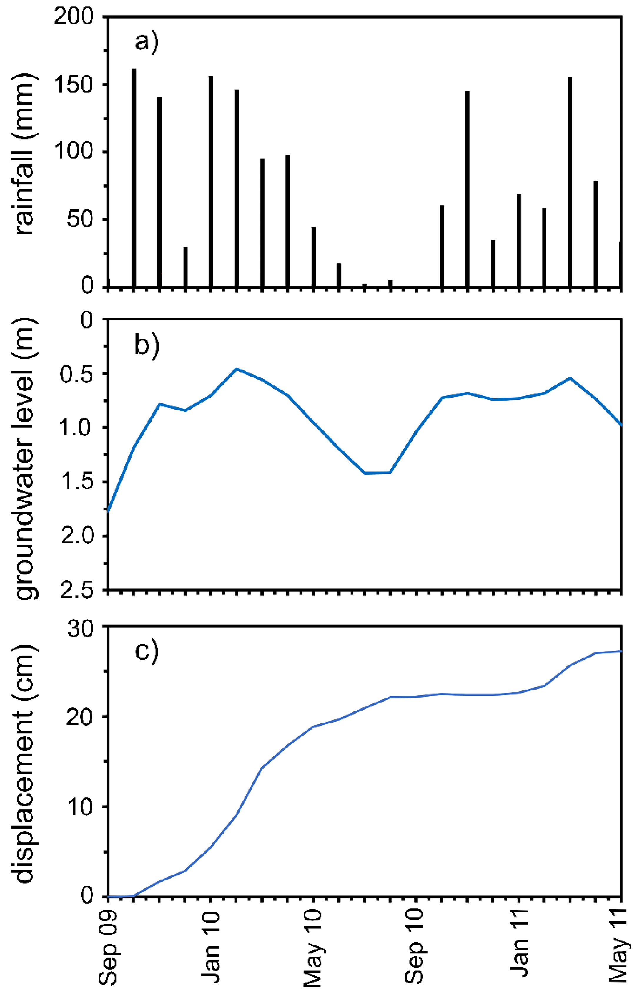
The approach presented in this study is employed in the present section to analyze the mobility of a landslide located near Palermo, in Sicily (Italy), which is named Cerda landslide (Figure 4a). A detailed documentation of this landslide can be found in Rosone et al. [39]. The Cerda landslide was triggered by an earthquake in 2002 and subsequently was seasonally reactivated owing to rainfall-induced fluctuations of water table. From the morphological viewpoint, the unstable soil mass was subdivided in three different bodies characterized by a different mobility (Figure 4b), as documented by Rosone et al. [39]. In the present study, attention is focused on the body named A (Figure 4b), which is characterized by an inclination angle of the ground surface of about 8°. The subsoil consists of a layer of weathered silty-clay overlying a formation of varicoloured clay (Figure 5a). The slip surface is located at the base of the upper layer and is characterized by a maximum depth of approximately 20 m below the ground surface. For the purposes of the present study, the unstable soil mass is schematized by two wedges bounded at their base by a bi-planar failure surface with β1 = 5° and β2 = 12° (Figure 5b). In autumn 2008, some piezometers and inclinometers along with a pluviometer were set up in the site affected by movements [39]. Rain recordings and groundwater level and horizontal displacements measurements are available from September 2009 to May 2011. These data are shown in Figure 6a–c from which it is clear that a noticeable simultaneity exists among rainfall, water-table fluctuations, and horizontal displacements.
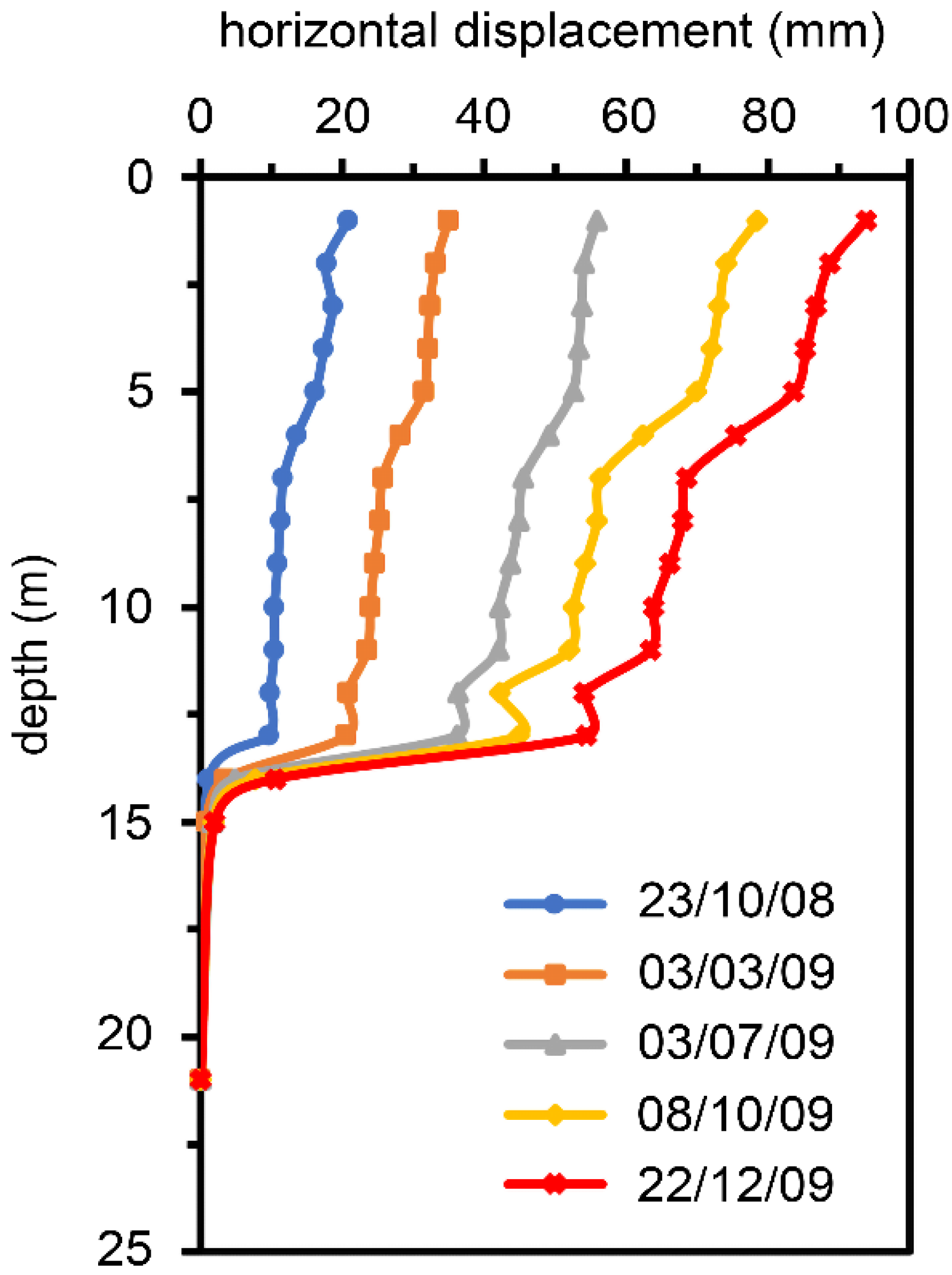
Figure 7 shows the available horizontal displacement profiles of inclinometer BH4 located at the toe of the landslide body (Figure 4b), as documented by Rosone et al. [39]. It is evident from Figure 7 that the soil deformations are essentially located within a well-defined zone situated below the layer of weathered silty-clay. This observation is consistent with the hypotheses on which the proposed approach is based. Shear strength parameters of the weathered silty-clay were obtained by Rosone et al. [39] by performing a large number of direct shear tests. Peak intercept cohesion and shearing resistance angle fall into the range 5–50 kPa and 22°–23°, respectively. An intercept cohesion equal to zero, and a friction angle were found at residual conditions. Considering that the Cerda landslide is periodically activated by rainfall, the residual strength parameters are employed in this work to characterize the soil shear strength in the shear zone. On the contrary, the peak shear strength parameters are employed for the soils forming the landslide body, considering that these soils are affected by moderate deformations. Therefore, it is assumed for the soil in correspondence of the interface between the two blocks (Figure 2). Soil unit weight is γ = 20.5 kN/m3 [40].
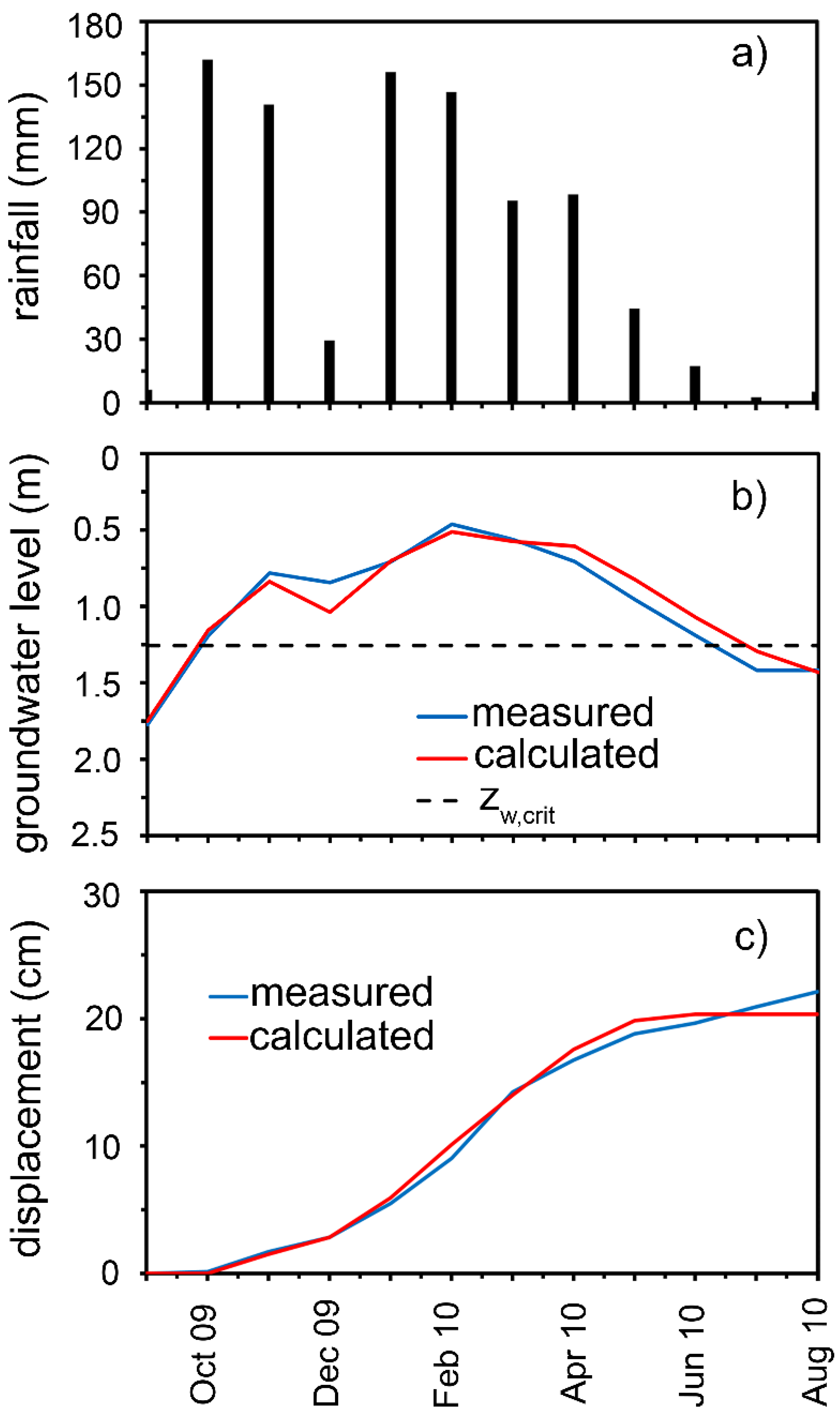
The remaining parameters involved in the proposed approach are calibrated using the above-mentioned procedure by matching the available recordings of water-table and soil displacement with the outcomes obtained using the proposed approach. In order to perform a reliable prediction of the landslide mobility, this calibration procedure should refer to a sufficiently prolonged time interval. To this purpose, the period from September 2009 to August 2010 is considered in the present study and from which the following parameters are obtained using Equation (1) along with rain recordings and groundwater level measurements: p = 161.9 mm/month, A = 0.27, and = 2.9 month−1. In addition, a coefficient of viscosity kN·month/m2 is evaluated on the basis of the soil displacements measured in the same time interval. The calibration results are reported in Figure 8a–c. It is clear from Figure 8b that the groundwater level calculated using the above-mentioned parameters well resembles the measured one. The critical level zw,crit (associated with force Ucrit) is also indicated in this figure for completeness. A reasonably fine accord between theoretical and observed soil displacements is also gained (Figure 8c). As a further requirement of the proposed method, area AA’A” (Figure 3) is calculated in the order of 10−3 m2. This value can be neglected in comparison with the total area of the entire unstable soil mass (12,000 m2).
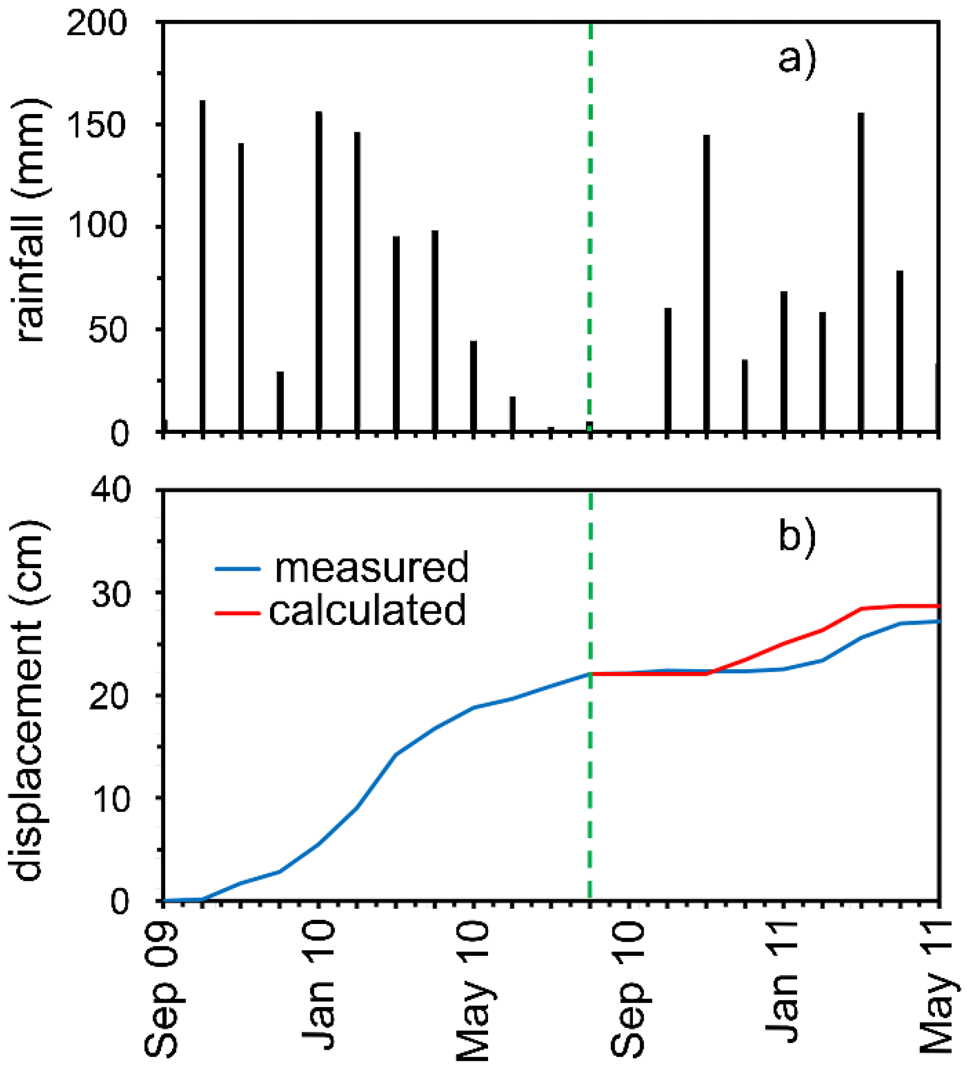
Once the calibration procedure is completed, the method is used to predict the displacement of the unstable soil mass in the subsequent period from August 2010 to May 2011. The beginning of the prediction is defined by a dashed line in Figure 9. A comparison between the calculated displacements and the recorded ones is reported in Figure 9b. The results of this comparison corroborate the predictive capacity of the approach proposed in the present study.
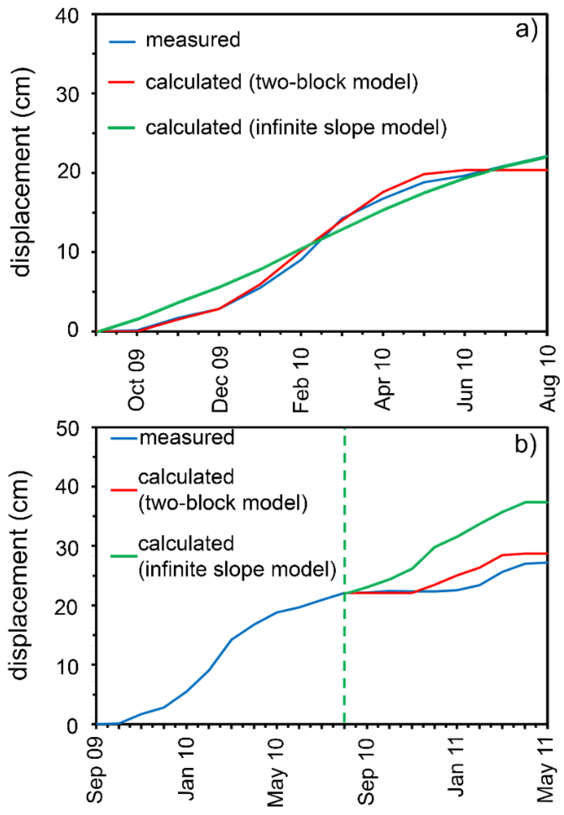
For the sake of completeness, a comparison between the present method and that developed by Conte et al. [34] using the simple infinite slope model is shown in Figure 10a,b. In this last method, it is assumed that the slip surface is located at a depth of 20 m from the ground surface and is parallel to the slope. Specifically, Figure 10a documents the results of the calibration stage, and Figure 10b shows the horizontal displacements predicted by the two methods on the basis of rainfall recorded from August 2010 to May 2011. It is evident from these figures that, for the considered case study, the predictive capacity of the proposed method is better than that of the method based on an infinite slope model that more roughly approximates the real geometry of the landslide body.
4. Conclusions
A simplified approach is proposed for predicting the movements undergone by the landslides cyclically activated by water-table changes owing to rain. The method uses some analytical equations relating pluviometric measurements to water-table oscillations and the latter to the mobility of the unstable soil mass. With this regard, a two-wedges model bounded at the bottom by a bi-planar failure surface is employed to schematize the unstable soil mass. The method requires few input parameters, most of which may be derived through traditional geotechnical tests. The remaining ones should be calibrated using the procedure that is incorporated in the method. The proposed approach is employed to analyze the mobility of a landslide documented in published papers, which is seasonally activated by water-table oscillations owing to rainfall. After calibrating some required parameters using the available groundwater table and landslide displacement measurements gathered from a sufficiently long period, the model is employed to estimate the movements of the unstable soil mass in a subsequent period using only rainfall recordings. The theoretical results are in good agreement with field observations. Although a more extensive validation is necessary, the proposed method seems to be promising from an engineering point of view to provide a preliminary prediction of the landslide mobility directly from expected rainfall scenarios.
Author Contributions
Conceptualization, A.T., E.C., and L.P.; methodology, A.T., E.C., and L.P.; software, L.P. and A.P.; formal analysis, L.P. and A.P.; writing—original draft preparation, A.T., E.C., and L.P.; writing—review and editing, A.T., E.C., and L.P.; visualization, A.P.; supervision, A.T. and E.C. All authors have read and agreed to the published version of the manuscript.
Funding
This research received no external funding.
Institutional Review Board Statement
Not applicable.
Informed Consent Statement
Not applicable.
Data Availability Statement
The data presented in this study are available on request from the corresponding author.
Conflicts of Interest
The authors declare no conflict of interest.
Appendix A
Under two-dimensional conditions, the viscous force F activated at the base of a landslide body during motion may be evaluated using the following equation derived from Bingham’s law:
where is the shear stress at the slip surface due to the soil viscosity, L is the length of this surface, is the soil viscosity, v is the velocity at the top of shear zone that is equal to the velocity of the moving soil mass (whereas v = 0 at the bottom of this zone), and d is the thickness of the shear zone. Therefore, F is a force for unit length in the normal direction to the cross-section of the slope. Considering the difficulties of experimentally evaluating and d, in the present study the following equation is used:
with
where can be considered as a model parameter to be calibrated using displacement measurements.
References
- Cruden, D.M.; Varnes, D.J. Landslides—Investigation and Mitigation; National Academy Press: Washington, DC, USA, 1996. [Google Scholar]
- Leroueil, S. Natural slopes and cuts: Movement and failure mechanisms. Géotechnique 2001, 51, 197–243. [Google Scholar] [CrossRef]
- Meyerhof, G.G.; Fellenius, B.H. Canadian Foundation Engineering Manual; Canadian Geotechnical Society: Calgary, Canada, 1985. [Google Scholar]
- Rampello, S.; Callisto, L.; Fargnoli, P. Evaluation of slope performance under earthquake loading conditions. Ital. Geotech. J. 2010, 4, 29–41. [Google Scholar]
- Jin, Y.-F.; Yin, Z.-Y.; Yuan, W.-H. Simulating retrogressive slope failure using two different smoothed particle finite element methods: A comparative study. Eng. Geol. 2020, 279, 105870. [Google Scholar] [CrossRef]
- Soga, K.; Alonso, E.; Yerro, A.; Kumar, K.; Bandara, S. Trends in large-deformation analysis of landslide mass movements with particular emphasis on the material point method. Géotechnique 2016, 66, 248–273. [Google Scholar] [CrossRef] [Green Version]
- Yerro, A.; Soga, K.; Bray, J.D. Runout evaluation of Oso landslide with the material point method. Can. Geotech. J. 2019, 56, 1304–1317. [Google Scholar] [CrossRef] [Green Version]
- Conte, E.; Pugliese, L.; Troncone, A. Post-failure analysis of the Maierato landslide using the material point method. Eng. Geol. 2020, 277, 105788. [Google Scholar] [CrossRef]
- Alonso, E.E. Triggering and motion of landslides. Géotechnique 2021, 71, 3–59. [Google Scholar] [CrossRef]
- Rohe, A.; Martinelli, M. Material point method and applications in geotechnical engineering. In Proceedings of the Workshop on Numerical Methods is Geotechnics, Hamburg, Germany, 27–28 September 2017; pp. 57–72. [Google Scholar]
- Fern, J.; Rohe, A.; Soga, K.; Alonso, E. The Material Point Method for Geotechnical Engineering. A Practical Guide, 1st ed.; CRC Press: Boca Raton, FL, USA, 2019. [Google Scholar]
- Van Asch, T.W.J.; Van Genuchten, P.M.B. A comparison between theoretical and measured creep profiles of landslides. Geomorphology 1990, 3, 45–55. [Google Scholar] [CrossRef]
- Di Maio, C.; Vassallo, R.; Vallario, M. Plastic and viscous shear displacements of a deep and very slow landslide in stiff clay formation. Eng. Geol. 2013, 162, 53–66. [Google Scholar] [CrossRef]
- Vulliet, L.; Hutter, K. Viscous-type sliding laws for landslides. Can. Geotech J. 1988, 25, 467–477. [Google Scholar] [CrossRef]
- Bracegirdle, A.; Vaughan, P.R.; High, D.W. Displacement prediction using rate effects on residual shear strength. In Proceedings of the 6th International Symposium on Landslides, Christchurch, New Zealand, 10 February 1992; Volume 1, pp. 343–348. [Google Scholar]
- Savage, W.Z.; Chleborad, A.F. A model for creeping flow in landslides. Bull. Assoc. Eng. Geol. 1982, 19, 333–338. [Google Scholar] [CrossRef]
- Desai, C.S.; Samtani, N.C.; Vulliet, L. Constitutive modeling and analysis of creeping soils. J. Geotech. Eng. ASCE 1995, 121, 43–56. [Google Scholar] [CrossRef]
- Van Asch, T.W.J.; Van Beek, L.P.H.; Bogaard, T.A. Problems in predicting the mobility of slow-moving landslides. Eng. Geol. 2007, 91, 46–55. [Google Scholar] [CrossRef]
- Olivella, S.; Gens, A.; Carrera, J.; Alonso, E.E. Numerical formulation for a simulator (CODE_BRIGHT) for the coupled analysis of saline media. Eng. Comput. 1996, 13, 87–112. [Google Scholar] [CrossRef] [Green Version]
- Ledesma, A.; Corominas, J.; Gonzàles, A.; Ferrari, A. Modelling slow moving landslides controlled by rainfall. In Proceedings of the 1st Italian Work Landslides, Napoli, Italy, 8–10 June 2009; Volume 1, pp. 196–205. [Google Scholar]
- Picarelli, L.; Urciuoli, G.; Russo, C. Effect of groundwater regime on the behaviour of clayey slopes. Can. Geotech. J. 2004, 41, 467–484. [Google Scholar] [CrossRef]
- Fernández-Merodo, J.A.; García-Davalillo, J.C.; Herrera, G.; Mira, P.; Pastor, M. 2D viscoplastic finite element modelling of slow landslides: The Portalet case study (Spain). Landslides 2014, 11, 29–42. [Google Scholar] [CrossRef]
- Hutchinson, J.N. A sliding-consolidation model for flow slides. Can. Geotech. J. 1986, 23, 115–126. [Google Scholar] [CrossRef]
- Gottardi, G.; Butterfield, R. Modelling 10 years of downhill creep data. In Proceedings of the 5th International Conference on Soil Mechanics and Geotechnical Engineering, Istanbul, Turkey, 27–31 August 2001; Volumes 1–3, pp. 27–31. [Google Scholar]
- Conte, E.; Troncone, A. Analytical method for predicting the mobility of slow-moving landslides owing to groundwater fluctuations. J. Geotech. Geoenviron. Eng. ASCE 2011, 137, 777–784. [Google Scholar] [CrossRef]
- Alonso, E.E.; Zervos, A.; Pinyol, N.M. Thermo-poro-mechanical analysis of landslides: From creeping behaviour to catastrophic failure. Géotechnique 2015, 63, 202–219. [Google Scholar] [CrossRef] [Green Version]
- Angeli, M.G.; Gasparetto, P.; Menotti, R.M.; Pasuto, A.; Silvano, S. A visco-plastic model for slope analysis applied to a mudslide in Cortina d’Ampezzo, Italy. Q. J. Eng. Geol. 1996, 29, 233–240. [Google Scholar] [CrossRef]
- Corominas, J.; Moja, J.; Ledesma, A.; Lloret, A.; Gili, J.A. Prediction of ground displacements and velocities from groundwater level changes at the Vallcebre landslide (Eastern Pyrenees, Spain). Landslides 2005, 2, 83–96. [Google Scholar] [CrossRef]
- Herrera, G.; Fernández-Merodo, J.A.; Mulas, J.; Pastor, M.; Luzi, G.; Monserrat, O.A. Landslide forecasting model using ground based SAR data: The Portalet case study. Eng. Geol. 2009, 105, 220–230. [Google Scholar] [CrossRef]
- Ranalli, M.; Gottardi, G.; Medina-Cetina, Z.; Nadim, F. Uncertainty quantification in the calibration of a dynamic viscoplastic model of slow slope movements. Landslides 2010, 7, 31–41. [Google Scholar] [CrossRef]
- Cascini, L.; Calvello, M.; Grimaldi, G.M. Displacement trends of slow-moving landslides: Classification and forecasting. J. Mt. Sci. 2014, 11, 592–606. [Google Scholar] [CrossRef]
- Cascini, L.; Calvello, M.; Grimaldi, G.M. Groundwater modeling for the analysis of active slow-moving landslides. J. Geotech. Geoenviron. Eng. (ASCE) 2010, 136, 1220–1230. [Google Scholar] [CrossRef]
- Bernardie, S.; Desramaut, N.; Malet, J.P.; Gourlay, M.; Grandjean, G. Prediction of changes in landslide rates induced by rainfall. Landslides 2015, 12, 481–494. [Google Scholar] [CrossRef] [Green Version]
- Conte, E.; Donato, A.; Troncone, A. A simplified method for predicting rainfall-induced mobility of active landslides. Landslides 2017, 14, 35–45. [Google Scholar] [CrossRef]
- Chowdhury, R.N. Slope Analysis. Developments in Geotechnical Engineering; Elsevier: Amsterdam, The Netherlands, 1978; Volume 22. [Google Scholar]
- Conte, E.; Troncone, A. A method for the analysis of soil slips triggered by rainfall. Géotechnique 2012, 62, 187–192. [Google Scholar] [CrossRef]
- Bandini, V.; Biondi, G.; Cascone, E.; Rampello, S. A GLE-based model for seismic displacement analysis of slopes including strength degradation and geometry rearrangement. Soil Dyn. Earthq. Eng. 2015, 71, 128–142. [Google Scholar] [CrossRef]
- Troncone, A.; Pugliese, L.; Lamanna, G.; Conte, E. Prediction of rainfall-induced landslide movements in the presence of stabilizing piles. Eng. Geol. 2021, 288, 106143. [Google Scholar] [CrossRef]
- Rosone, M.; Ziccarelli, M.; Ferrari, A.; Airò Farulla, C. On the reactivation of a large landslide induced by rainfall in highly fissured clays. Eng. Geol. 2018, 235, 20–38. [Google Scholar] [CrossRef]
- Rosone, M.; Ziccarelli, M.; Ferrari, A. Displacement evolution of a large landslide in a highly fissured clay. In Geotechnical Research for Land Protection and Development CNRIG 2019. Lecture Notes in Civil Engineering; Calvetti, F., Cotecchia, F., Galli, A., Jommi, C., Eds.; Springer: Berlin/Heidelberg, Germany, 2020; Volume 40, pp. 195–204. [Google Scholar]
Figure 1.
Schematization of the unstable soil mass with a two-wedges model.

Figure 2.
Forces acting on the wedges.

Figure 3.
Schematization of the kinematical mechanism of the two blocks. The area AA’A”, the horizontal component of the soil displacement d, and the velocities of the wedges v1 and v2 are indicated.
Figure 3.
Schematization of the kinematical mechanism of the two blocks. The area AA’A”, the horizontal component of the soil displacement d, and the velocities of the wedges v1 and v2 are indicated.

Figure 4.
Cerda landslide: (a) location of the Cerda village; (b) plan of the landslide site with an indication of the landslide body considered in the present study (landslide A) and the location of the field test carried out.
Figure 4.
Cerda landslide: (a) location of the Cerda village; (b) plan of the landslide site with an indication of the landslide body considered in the present study (landslide A) and the location of the field test carried out.

Figure 5.
Section A-A’ of the Cerda landslide, whose trace is shown in Figure 4b: (a) longitudinal section of the slope; (b) bi-planar surface used in the present study to approximate the slip surface.
Figure 5.
Section A-A’ of the Cerda landslide, whose trace is shown in Figure 4b: (a) longitudinal section of the slope; (b) bi-planar surface used in the present study to approximate the slip surface.

Figure 6.
Available measurements from September 2009 to May 2011: (a) rainfall, (b) groundwater level, (c) displacement.
Figure 6.
Available measurements from September 2009 to May 2011: (a) rainfall, (b) groundwater level, (c) displacement.

Figure 7.
Horizontal displacement profiles recorded at the head of inclinometer BH4 located in the landslide body, whose position is indicated in Figure 4b.
Figure 7.
Horizontal displacement profiles recorded at the head of inclinometer BH4 located in the landslide body, whose position is indicated in Figure 4b.

Figure 8.
Comparison between observed and calculated results: (a) rain recordings, (b) groundwater level fluctuations with the indication of its critical position, (c) soil displacement in the horizontal direction. All data refer to the period from September 2009 to August 2010.
Figure 8.
Comparison between observed and calculated results: (a) rain recordings, (b) groundwater level fluctuations with the indication of its critical position, (c) soil displacement in the horizontal direction. All data refer to the period from September 2009 to August 2010.

Figure 9.
Prediction of soil displacement carried out by means of the proposed approach, referring to the time period from August 2010 to May 2011: (a) rain recordings, (b) horizontal displacement. The dotted line indicates the beginning of prediction.
Figure 9.
Prediction of soil displacement carried out by means of the proposed approach, referring to the time period from August 2010 to May 2011: (a) rain recordings, (b) horizontal displacement. The dotted line indicates the beginning of prediction.

Figure 10.
Comparison between the results obtained using the two-blocks model proposed in the present study and a simpler infinite slope model [34]: (a) calibration stage, (b) prediction stage. The dotted line in (b) indicates the beginning of prediction.
Figure 10.
Comparison between the results obtained using the two-blocks model proposed in the present study and a simpler infinite slope model [34]: (a) calibration stage, (b) prediction stage. The dotted line in (b) indicates the beginning of prediction.

Publisher’s Note: MDPI stays neutral with regard to jurisdictional claims in published maps and institutional affiliations. |
© 2021 by the authors. Licensee MDPI, Basel, Switzerland. This article is an open access article distributed under the terms and conditions of the Creative Commons Attribution (CC BY) license (https://creativecommons.org/licenses/by/4.0/).
Share and Cite
MDPI and ACS Style
Troncone, A.; Pugliese, L.; Parise, A.; Conte, E. Prediction of Slow-Moving Landslide Mobility Due to Rainfall Using a Two-Wedges Model. Water 2021, 13, 2030. https://doi.org/10.3390/w13152030
AMA Style
Troncone A, Pugliese L, Parise A, Conte E. Prediction of Slow-Moving Landslide Mobility Due to Rainfall Using a Two-Wedges Model. Water. 2021; 13(15):2030. https://doi.org/10.3390/w13152030
Chicago/Turabian StyleTroncone, Antonello, Luigi Pugliese, Andrea Parise, and Enrico Conte. 2021. "Prediction of Slow-Moving Landslide Mobility Due to Rainfall Using a Two-Wedges Model" Water 13, no. 15: 2030. https://doi.org/10.3390/w13152030
Note that from the first issue of 2016, this journal uses article numbers instead of page numbers. See further details here.