Evaluation of Evapotranspiration in Brazilian Cerrado Biome Simulated with the SWAT Model

Abstract

Evapotranspiration represents a significant part on the water balance and, thus, the correct evaluation of this hydrological parcel is relevant when modeling a watershed. The objective of this work is to evaluate the Soil and Water Assessment Tool (SWAT) model’s capability in adequately simulating evapotranspiration in a watershed with predominance of the Brazilian Cerrado biome. Hydrological modeling of the Gama watershed located in the Federal District, which has 57.5% of its total area covered by pristine Cerrado, was conducted. Hydrometeorological and turbulent flow variables have been monitored in weather station and Eddy Covariance (EC) tower, respectively. SWAT simulations were performed for potential evapotranspiration methods: Hargreaves (H), Priestley–Taylor (PT) and Penman–Monteith (PM). Modified versions of SWAT for estimating actual (ET) by Strauch and Volk (2013) (SV) and Arroio Junior (2016) (AR) were also tested. The calibration and verification of the SWAT model, in terms of daily flow, were carried out using a Particle Swarm Optimization algorithm, and fair results were obtained with all the methods evaluated. The actual evapotranspiration (ET) simulated with SWAT (ETsim) using the PM, PT, H, SV and AR methods for a Cerrado hydrological response unit (HRU) were evaluated and compared with the ET obtained using the turbulent flow (Eddy Covariance) method (ETobs). Comparing ETobs and ETsim results, the PM method showed the best fitness and the H and PT methods showed better fit for the dry and the rainy periods, respectively. Although representing an advance on ET modeling, the SV and AR modifications did not improve the response in terms of simulation of the studied area.

1. Introduction

Evapotranspiration combines water losses to the atmosphere through soil evaporation and vegetation transpiration, and represents the second most important component in the assessment of the hydrological cycle [1]. Despite this, determining evapotranspiration using hydrological models is still a challenge, especially due to the limited availability of evapotranspiration data or meteorological variables necessary for its estimation [2,3,4,5]. Another obstacle is the selection of the appropriate method to represent the complexity of this process in hydrological models [5,6,7,8].

The hydrological models represent the hydrological processes by mathematical functions with parameters that do not always have physical meaning. This happens not only due to deficiencies in the model formulation and structure itself, but also because of difficulties in estimating representative parameters for the physical processes due to local conditions and spatial variability, and thus, calibration using observed data such as flow rates is usually used to adjust the model parameters. In this way, errors in the ET estimation can be “corrected” by the model with the aim of obtain a series of flows that are close to the series of observed flows. The literature presents some discussions regarding the results of conceptual models, emphasizing that these models do not always generate the correct results for the correct reasons [9,10,11].

Hydrological rainfall- runoff models estimate actual evapotranspiration (ET) based on potential evapotranspiration (PET). The Soil and Water Assessment Tool (SWAT model), for example, offers three methods for determining PET and later estimating ET: Penman–Monteith [12], Priestley–Taylor [13] and the Hargreaves [14]. Developed by the USDA Agricultural Research Service (ARS), SWAT is a useful tool in understanding the components of the hydrological cycle and assessing the impact of different soil uses in relation to flows and/or sediment [15,16,17].

In most rainfall–runoff studies, there is usually no assessment of the accuracy of PET or ET estimates. However, as Strauch and Volk [18] emphasize, even though a considerable number of studies has used the SWAT model for Brazilian basins and presented simulations with calibrations considered good or satisfactory for the flow and/or sediments, these results do not necessarily guarantee that hydrological processes are being correctly simulated. In this perspective, Melo Neto [19] and Castro [20] found underestimation of evapotranspiration in simulations using SWAT, in the Atlantic Forest and Cerrado biomes, under climatic conditions defined by Koppen, Cwa and Aw, respectively.

The applicability of PET determination methods must be considered. Oudin et al. [21], trying to identify the best method for estimating PET in rainfall–runoff models, concluded that a simple PET estimate, based on temperature, works just as well as the Penman–Monteith model. As a result, Oudin et al. [21] questioned: “if a simple temperature-based PET estimation works as well as a Penman-type model, why not use a simpler model with lower data requirements?”. Kannan et al. [22], evaluating a combination of methods for generating ET and flow, concluded that the Hargreaves method, using temperature, presented results as adequate as the more complex method of Penman–Monteith, considering energy balance, on a daily scale.

There are limitations associated with estimating ET based on PET; therefore, in order to improve the representativeness of evapotranspiration, Strauch and Volk [18] implemented two new parameters (TRAMO1 and TRAMO2) in the SWAT model code. TRAMO1 and TRAMO2 define, respectively, the first and the last month of a transition period from the dry to the rainy season, making it possible that short periods of drought during the rainy season or single rainfall events at the beginning of a dry season do not provoke the end/start of a plant growing season. Similarly, the study by Arroio Junior [23] changed a code routine, so that the plant dormancy mechanism that exists in the standard SWAT model was completely deactivated. It is worth mentioning that the modifications in the model code, made by the authors Strauch and Volk [18] and Arroio Junior [23], only impact the way in which SWAT calculates the ET, with the PET method used in both studies being the Penman–Monteith method.

In this regard, this work evaluated the potential of the SWAT model in simulating the evapotranspiration of tropical basins with pristine Cerrado biome, the most extensive Brazilian savanna. Three methods of estimating potential evapotranspiration provided by the SWAT model and two modified actual evapotranspiration estimation strategies, proposed by Strauch and Volk [18] and Arroio Junior [23], were tested. Ribeirão do Gama-DF basin, which has 57.5% of its total area covered by pristine Cerrado, was chosen for the available long term hydrometeorological data and two Eddy Covariance monitoring towers.

2. Materials and Methods

2.1. Study Area

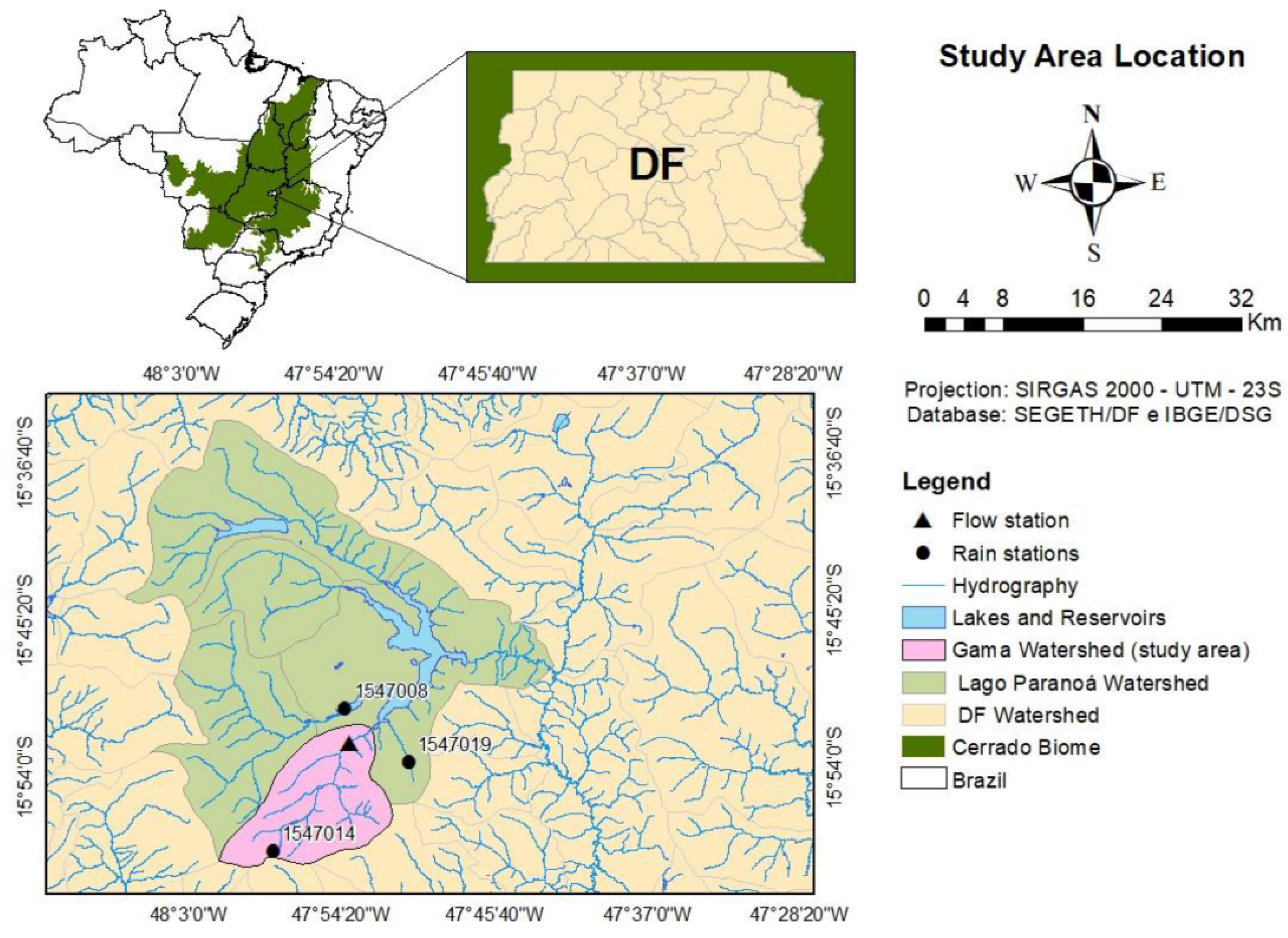
The study area is the Ribeirão do Gama basin, located in the southern portion of the Federal District (DF) (Figure 1). Ribeirão do Gama is an important tributary of Paranoá Lake, with a mean flow of 2.90 m³/s. Cerrado is the predominant land cover in the Ribeirão do Gama basin, representing 57.5% of the total area, in addition to the occurrence of urban (23.28%), rural (3.73%) and other occupations (15.49%) (Figure 2D). Regarding pedology, the Red Latosols (46.4%) and Red Yellow Latosols (19.3%) predominate, in addition to Cambisols (18.3%), Gleisols (15.7%) and Plintosols (0.3%) (Figure 2C). The climate in the study area is tropical Aw, defined by Koppen as typical of savannas, with monthly mean temperature and evapotranspiration equal to 22 °C and 65 mm, respectively, and annual precipitation of approximately 1500 mm distributed between October and March [24].

2.2. Hydrological Modelling

The SWAT model was used for hydrological simulation of the basin with daily time steps [15,25]. The spatial distribution of the SWAT is represented by segmentations of the basin into sub-basins, based on topography, and finally, into Hydrological Response Units (HRUs), which consist of unique conditions of soil type, land use and the topographic [26].

SWAT models estimates evapotranspiration by separately considering the evaporation processes of rivers, soil and vegetated surfaces and the transpiration process of plants. After determining the potential evapotranspiration, the actual evapotranspiration is calculated; SWAT first evaporates any precipitation intercepted by the plant canopy, then computes the maximum amount of transpiration and the maximum amount of soil evaporation using a similar approach that of Richtie [27]. Then, the actual amount of evaporation from the soil is obtained, which will be influenced by the rate of shading.

However, when there is a demand for water evaporation from the soil, the SWAT first partitions the evaporative demand between the different layers; the evaporative demand not used by a soil layer results in a reduction in the actual evapotranspiration for HRU. Finally, the actual transpiration is estimated, which, in addition to being a function of potential transpiration and the availability of water in the soil, is directly linked to the leaf area index, which, in turn, is related to the plant’s development stage [26].

To determine potential evapotranspiration (PET), which is equivalent to the evapotranspiration rate limited only by the energy available in a system [28], SWAT offers three standard methods: the Penman–Monteith method [12], the Priestley–Taylor method [13] and the Hargreaves method [14] (

Table 1. Potential evapotranspiration models evaluated.

Potential Evapotranspiration Methods	Equation
Penman–Monteith	$\mathsf{\lambda }\mathrm{E}=\frac{∆·\left({\mathrm{H}}_{\mathrm{net}}-\mathrm{G}\right)+{\mathsf{\rho }}_{\mathrm{air}}·{\mathrm{c}}_{\mathrm{p}}·\left[{\mathrm{e}}_{\mathrm{z}}^{\mathrm{o}}-{\mathrm{e}}_{\mathrm{z}}\right]/{\mathrm{r}}_{\mathrm{a}}}{∆+\mathsf{\gamma }·\left(1+{\mathrm{r}}_{\mathrm{c}}/{\mathrm{r}}_{\mathrm{a}}\right)}$
Priestley–Taylor	${\mathsf{\lambda }\mathrm{E}}_{\mathrm{o}}={\mathsf{\alpha }}_{\mathrm{pet}}·\frac{∆}{∆+\mathsf{\gamma }}·\left({\mathrm{H}}_{\mathrm{net}}-\mathrm{G}\right)$
Hargreaves	${\mathsf{\lambda }\mathrm{E}}_0=0.0023·{\mathrm{H}}_0·{\left({\mathrm{T}}_{\mathrm{mx}}-{\mathrm{T}}_{\mathrm{mn}}\right)}^{0.5}·\left(\overline{{\mathrm{T}}_{\mathrm{av}}}+17.8\right)$

). The model also provides the option for the user to enter the calculated PET data in case they want to use any method other than the model’s standards.

In which: $\mathsf{\lambda }\mathrm{E}$ is the latent heat flux density (MJ·m⁻²·d⁻¹), λ is the latent heat of vaporization (MJ·kg⁻¹), E is the depth rate evaporation (mm·d⁻¹), $∆$ is the slope of the saturation vapor pressure–temperature curve (de/dT) (kPa·°C⁻¹), ${\mathrm{H}}_{\mathrm{net}}$ is the net radiation (MJ·m⁻²·d⁻¹), G is the heat flux density to the ground (MJ·m⁻²·d⁻¹), ${\mathsf{\rho }}_{\mathrm{air}}$ is the air density (kg·m⁻³), ${\mathrm{c}}_{\mathrm{p}}$ is the specific heat at constant pressure (MJ·kg⁻¹·°C⁻¹), ${\mathrm{e}}_{\mathrm{z}}^{\mathrm{o}}$ is the saturation vapor pressure of air at height z (kPa), ${\mathrm{e}}_{\mathrm{z}}$ is the water vapor pressure of air at height z (kPa), γ is the psychrometric constant (kPa·°C⁻¹), ${\mathrm{r}}_{\mathrm{c}}$ is the plant canopy resistance (s·m⁻¹), ${\mathrm{r}}_{\mathrm{a}}$ is the diffusion resistance of the air layer (aerodynamic resistance) (s·m⁻¹), E_o is the potential evapotranspiration (mm·d⁻¹), ${\mathsf{\alpha }}_{\mathrm{pet}}$ is a coefficient, ${\mathrm{H}}_0$ is the extraterrestrial radiation (MJ·m⁻²·d⁻¹), ${\mathrm{T}}_{\mathrm{mx}}$ is the maximum air temperature for a given day (°C), ${\mathrm{T}}_{\mathrm{mn}}$ is the minimum air temperature for a given day (°C), and $\overline{{\mathrm{T}}_{\mathrm{av}}}$ is the mean air temperature for a given day (°C).

Evapotranspiration is associated with plant growth; in SWAT, the plant growth module is a simplification of the “Environmental Policy Impact Climate” (EPIC) crop growth module [29,30], which was developed to support soil erosion assessments of the impacts of soil productivity on the soil, climate, and growing conditions of agricultural production regions in the United States [31]. SWAT uses EPIC’s phenological plant development concepts based on daily cumulative heat units. Thus, for plant growth, a certain thermal accumulation is necessary, represented by the sum of the difference between the average daily temperatures and the base temperature.

In line with the research of Strauch and Volk [18], as a means to consider soil moisture as a trigger for vegetation growth and not temperature, as considered in the default SWAT simulation, the available water for the plant was used, and was simulated in the upper layers of the soil, as a stimulus for new growth cycles. However, during the dry season, soils, or at least their upper horizons, usually dry up to the wilting point. However, new SWAT growing seasons should begin as soon as the simulated soil moisture effectively increases after the dry season. Thus, to ensure that short periods of drought during the rainy season or single rainfall events at the beginning of a dry season do not cause the end/beginning of a growing season, two new parameters, TRAMO1 and TRAMO2, which define the first and last month of a transition period, transition from the dry to the rainy season. According to the equinoxes, the default values for TRAMO1 and TRAMO2 were on 3 (March) and 4 (April) in the northern hemisphere and 8 (August) and 9 (September) in the southern hemisphere, respectively. In addition, Strauch and Volk [1] performed a modification in the rate of the leaf area index (LAI) decline using a logistic function combining the sigmoidal increase in the ideal LAI curve with a similar sigmoidal decline (for more information, see Strauch and Volk [18]).

In plant growth, the default SWAT program has the dormancy mechanism, a period in which there is no plant growth. In SWAT, dormancy occurs when the length of the day approaches the minimum for the year. Then, a fraction of the biomass is converted to residue and the LAI is set to a plant-specific minimum value.

However, in its Arroio Junior [23] modification, it is considered that the LAI reduction does not reflect the development cycle of plants from tropical and sub-tropical environments, and that the range of possible values of alteration by the default SWAT is not adequate to represent the plant growth dynamics in tropical zones, since it still induces a significant reduction in the LAI in the months of shorter photoperiod. From this perspective, Arroio Junior [23] modified the dormant.f subroutine, responsible for checking the dormancy state of different types of plants. By making this modification in the plant growth routines in the model’s source code, the dormancy mechanism was deactivated.

2.3. Model Data Inputs

Initially, the necessary database for the SWAT model simulation was structured. The land use and land cover map (Figure 2D) elaborated by Nunes [32] was used. The pedology map (Figure 2C) is based on the work of Reatto et al. [33]. Topographic, pedological and land use and land cover similarities resulted in 467 HRUs (Figure 2E).

Precipitation data were collected in three rainfall gauging stations: (Figure 1) Cabeça de Veado ETA (Estação de tratamento de água, which means water treatment plant), ETE (Estação de tratamento de esgoto, which means wastewater treatment plant) Sul and Área Alfa. The streamflow data used to calibrate the simulations were obtained from a stage-streamflow gaging station (Figure 1).

A turbulent flow tower (Eddy Covariance, EC) is installed at a height of 12 m in a pristine Cerrado area (Figure 2E), which provided meteorological data, such as temperature (°C), relative humidity (%), short-wave solar radiation (MJ·m⁻²·d), wind speed (ms⁻¹), solar radiation fluxes (MJ·m⁻²·d) and latent heat (LE, MJ·m⁻²·d), on a daily scale. The ratio between LE and the latent heat of vaporization (λ = 2.5 MJ·kg⁻¹) resulted in the observed ET values and they were used for comparison with the simulated ET values.

2.4. Stream Flow Calibration

Simulations were performed with the SWAT model in the default mode in order to test the available methods for determining potential evapotranspiration. In addition to the standard methods provided by SWAT (Penman–Monteith, Priestley–Taylor and Hargreaves), simulations were made using the codes modified by Strauch and Volk [1] and Arroio Junior [23]. These modifications, adopted to improve the evapotranspiration estimates, could be implemented in this work due to the open code of the SWAT model.

The simulations were calibrated in terms of flow in daily mode, in the period from 2013 to 2015, and verification was also conducted in daily mode in the period from 2016 to 2017 with each of the five selected methodologies. With a 3-year warm-up period, about 2000 simulation runs were executed for each evaluated method, using a Particle Swarm Optimization algorithm, implemented in a code prepared by Távora [34]. The parameters chosen for calibration were selected based on Sarmento [35], Ferrigo [36,37,38,39], Arnold et al. [15], Salles [40], Strauch and Volk [18], Nunes [32] and Arroio Junior [23] (see

Table 2. Parameters used in calibration.

Parameters	Description	Range
ALPHA_BF	Baseflow alpha factor (days)	0–1
ALPHA_BNK	Baseflow alpha factor for bank storage (days)	0–1
CANMX	Maximum canopy storage (mm H2O)	0–100
CH_K2	Effective hydraulic conductivity in main channel alluvium (mm/h)	−0.01–500
CH_N2	Manning’s “n” value for the main channel	−0.01–0.3
CN2	Initial SCS runoff curve number for moisture condition II	0.1–1.5 *
DEEPST	Initial depth of water in the deep aquifer (mm H2O)	0–50,000
EPCO	Plant uptake compensation factor	0–1
ESCO	Soil evaporation compensation factor	0–1
GW_DELAY	Groundwater delay time (days)	0–500
GW_REVAP	Groundwater revap (water in the shallow aquifer returning to the root zone) coefficient.	0.02–2
GWHT	Initial groundwater height (m).	0–25
GWQMN	Threshold depth of water in the shallow aquifer required for return flow to occur (mm H2O)	0–5000
OV_N	Manning’s “n” value for overland flow	0.01–30
RCHRG_DP	Deep aquifer percolation fraction.	0–1
REVAPMN	Threshold depth of water in the shallow aquifer for “revap” or percolation to the deep aquifer to occur (mm H2O)	0–500
SHALLST	Initial depth of water in the shallow aquifer (mm H2O)	0.05–24
SURLAG	Surface runoff lag coefficient	0–50,000

* Calibration changed by multiplying factor.

).

The five methods have been independently calibrated and verified in terms of flow. However, as the modified versions of Strauch and Volk [18] (SV) and Arroio Junior [23] (AR) use Penman–Monteith (PM) as their PET method, we tried to apply the PM calibrated parameters to these methods. Even so, for the SV and AR methods, independent calibrations were performed. With the simulations calibrated and verified in terms of flow for all evaluated methods, the evapotranspiration analysis was performed by comparing the simulated actual evapotranspiration data (ETsim) to the ET values obtained by Eddy Covariance (EC) at the turbulent flow tower.

2.5. Model Performance Evaluation

Furthermore, to evaluate the fit between the simulated and observed flow data, both in the calibration and in the validation step, graphical evaluation techniques were used, through the plotted hydrographs, in addition to the coefficient values of Nash–Sutcliffe Efficiency for the flow logarithm (Log NSE) (Equation (1)) and Trend Percentage (PBIAS) (Equation (2)). To compare the results of actual evapotranspiration simulated by SWAT and observed through EC, the following metrics were used: mean absolute error (MAE) in mm per day (Equation (3)), mean square root of the error (RMSE) in mm per day (Equation (4)) and correlation coefficient (R) (Equation (5)).

$$\mathrm{Log}\mathrm{NSE}=1-\frac{{\sum }_{\mathrm{i}=1}^{\mathrm{n}}{({\mathrm{LogV}}_{\mathrm{obs}}-{\mathrm{LogV}}_{\mathrm{sim}})}^2}{{\sum }_{\mathrm{i}=1}^{\mathrm{n}}{({\mathrm{LogV}}_{\mathrm{obs}}-\mathrm{Log}\overline{{\mathrm{V}}_{\mathrm{obs}}})}^2}$$

(1)

$$\mathrm{PBIAS}=\frac{{\sum }_{\mathrm{i}=1}^{\mathrm{n}}({\mathrm{V}}_{\mathrm{obs}}-{\mathrm{V}}_{\mathrm{sim}})·100}{{\sum }_{\mathrm{i}=1}^{\mathrm{n}}{\mathrm{V}}_{\mathrm{obs}}}$$

(2)

$$\mathrm{MAE}=\frac{{\sum }_{\mathrm{i}=1}^{\mathrm{n}}\left|\left({\mathrm{V}}_{\mathrm{sim}}-{\mathrm{V}}_{\mathrm{Obs}}\right)\right|}{\mathrm{n}}$$

(3)

$$\mathrm{RMSE}=\sqrt{\frac{{\sum }_{\mathrm{i}=1}^{\mathrm{n}}{\left({\mathrm{V}}_{\mathrm{sim}}-{\mathrm{V}}_{\mathrm{Obs}}\right)}^2}{\mathrm{n}}}$$

(4)

$$\mathrm{R}=\frac{{\sum }_{\mathrm{i}=1}^{\mathrm{n}}[\left({\mathrm{V}}_{\mathrm{sim}}-\overline{{\mathrm{V}}_{\mathrm{sim}}}\right)\left({\mathrm{V}}_{\mathrm{Obs}}-\overline{{\mathrm{V}}_{\mathrm{Obs}}}\right)]}{\sqrt{[{\sum }_{\mathrm{i}=1}^{\mathrm{n}}{\left({\mathrm{V}}_{\mathrm{sim}}-\overline{{\mathrm{V}}_{\mathrm{sim}}}\right)}^2][{\sum }_{\mathrm{i}=1}^{\mathrm{n}}{\left({\mathrm{V}}_{\mathrm{Obs}}-\overline{{\mathrm{V}}_{\mathrm{Obs}}}\right)}^2]}}$$

(5)

in which: ${\mathrm{V}}_{\mathrm{obs}}$ is the observed variable, ${\mathrm{V}}_{\mathrm{sim}}$ is the variable simulated by the model, $\overline{{\mathrm{V}}_{\mathrm{obs}}}$ is the mean of the observed variable during the simulated period, $\overline{{\mathrm{V}}_{\mathrm{sim}}}$ is the mean of the variable simulated by the model, $\overline{{\mathrm{V}}_{\mathrm{Obs}}}$ is the mean of the observed variable and n is the number of events considered.

To reduce quadratic differences and sensitivity to extreme values, NSE is often calculated with log values from observed and simulated data [41]. NSE is more influenced by peak values, whereas the logarithm of the variable (Log NSE) reduces this influence and emphasizes low values that occur in dry seasons. In the present study, as the focus is on evapotranspiration, the errors that occurred in the maximum flow values are of less interest because they occurred in events in which evapotranspiration had little influence. The Trend Percentage (PBIAS) measures the average trend of the simulated data to be higher or lower than the observed counterparts. The Mean Absolute Error (MAE) and Root Mean Square Error (RMSE) are measures of model performance that summarize the mean difference in the observed and simulated evapotranspiration data. Correlation coefficients were used to measure how strong a relationship is between two observed and simulated variables of evapotranspiration.

3. Results and Discussion

3.1. Model Calibration Strategies and Validation

Initially, calibration and verification, in terms of flow, were performed with daily time steps using the Penman–Monteith (PM), Priestley–Taylor (PT) and Hargreaves (H) methods. Statistical coefficients that were representative of model performance were considered for flow simulation.

Table 3. Calibration and Verification Statistical Metrics for the simulated PM, PT and H methods and for the SV and AR modifications using the SWAT parameters obtained in the calibration for the PM method and for SV and AR independently.

Methods	Calibration		Verification
	LogNSE	PBIAS (%)	LogNSE	PBIAS (%)
Penman–Monteith	0.88	−8.00	0.78	17.80
Priestley–Taylor	0.87	−5.40	0.32	43.00
Hargreaves	0.78	−2.30	0.53	−13.80
Strauch and Volk [18] + PM parameters	0.81	4.10	0.59	23.60
Strauch and Volk [18]	0.89	−1.50	0.72	23.30
Arroio Junior [23] + PM parameters	0.55	28.90	0.33	51.00
Arroio Junior [23]	0.89	0.78	0.63	33.30

presents the metrics obtained for calibration and verification for the PM, PT, and H methods. Good performance was achieved in the calibration process with LogNSE ranging from 0.78 to 0.88.

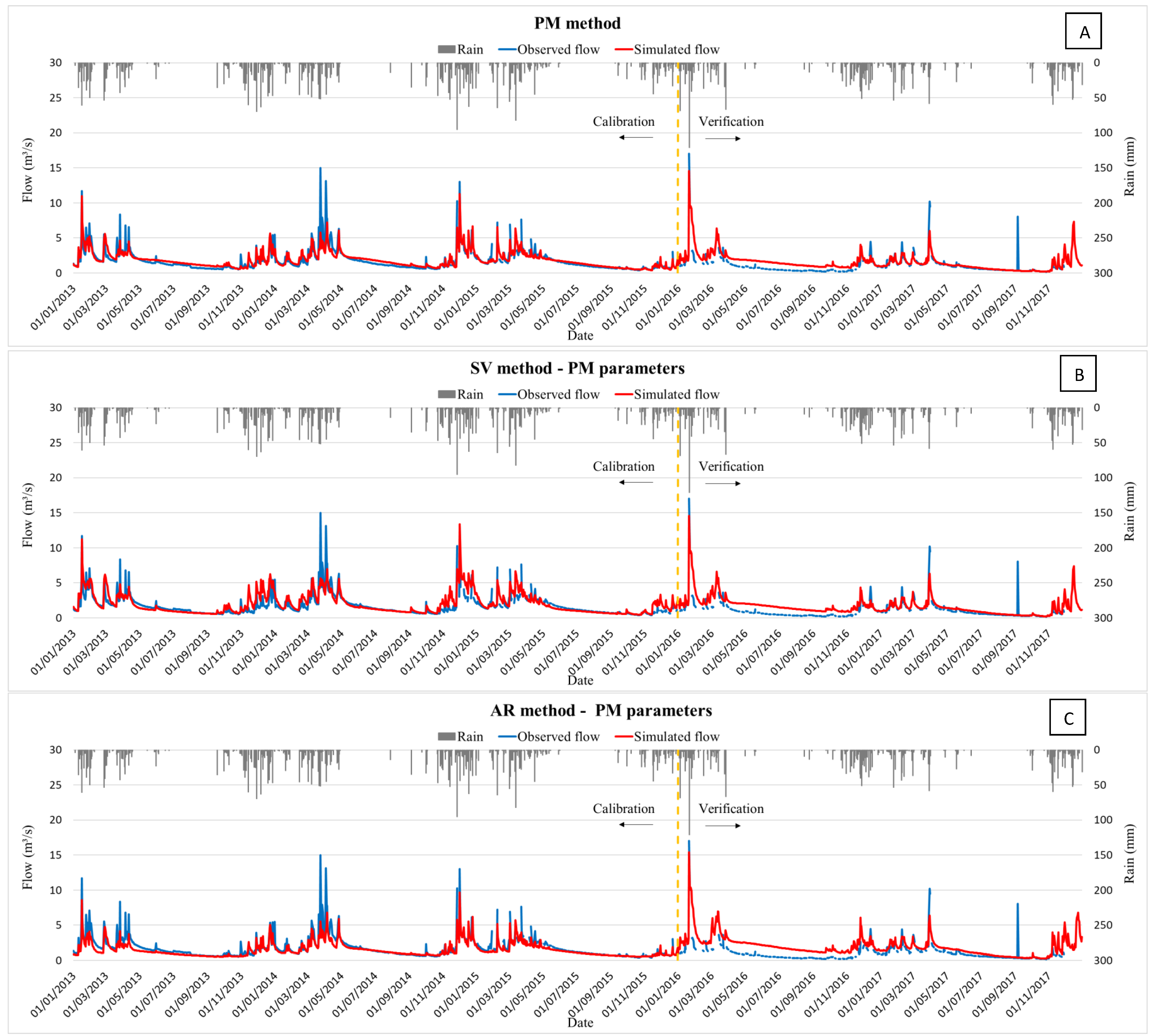
To evaluate the actual evapotranspiration simulated for the Cerrado at the HRU level, optimal parameters obtained for the simulation with the PM method were adopted (Figure 3A) for the modifications proposed by Strauch and Volk [18] (SV) and Arroio Junior [23] (AR), without new parameter calibration, to verify if the modifications could improve the PM method’s simulations. Thus, the optimal set of PM parameters were used in the modified algorithms of SV (Figure 3B) and AR (Figure 3C). In sequence, the SWAT parameters for PM method with SV and AR modifications were independently calibrated and the results are shown for the SV (Figure 4A) and AR (Figure 4B) modifications. Table 3 presents the statistical coefficients for these mentioned scenarios.

The visual analysis of the graphs indicates that the simulations, in general, exhibited a similar behavior between the observed and simulated hydrographs, following the baseflows in both the rainy and dry seasons. However, there are peaks in the observed data that were not correctly simulated, but this can be caused by the fact that it is an assessment at a daily level, and the observed flow data are calculated at a momentary flood moment, since the flows are measured from two daily readings of the stage.

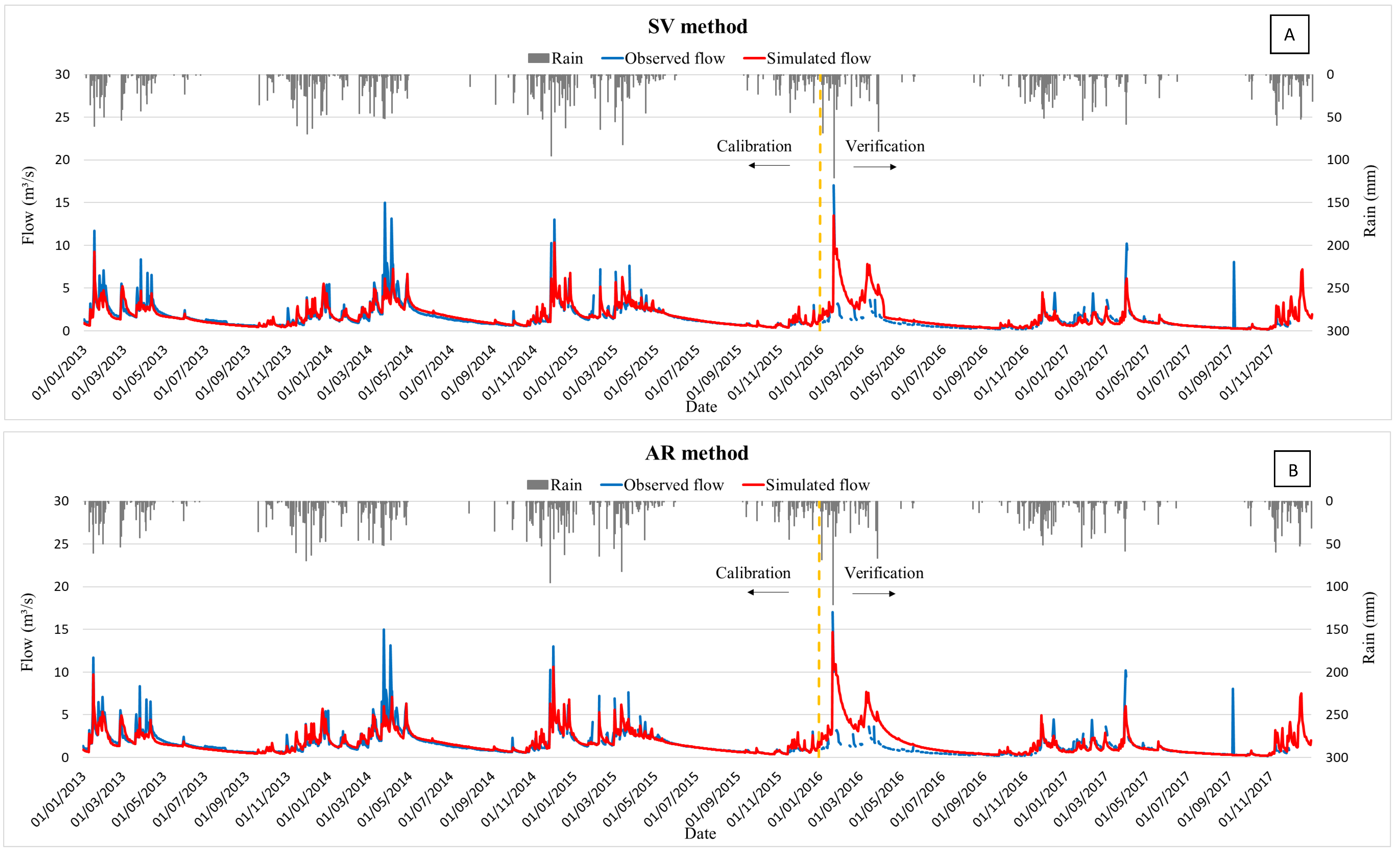
It was noted that there was a slight deterioration in the recession period simulations for the SV and AR modifications with the application of the PM parameters. It is verified that the SV and AR modifications with the application of the PM parameters worsen the results compared to the original PM method. This fact showed that the hypothesis that improvements could occur with the modifications using the parameters calibrated for the PM method was not confirmed. It is noticed that the LogNSE and PBIAS values are higher for the independent calibrations with the SV and AR modifications, and it was, therefore, decided to use the parameters obtained by these independent calibrations of each evaluated methodology in order to proceed with the evaluation of the actual evapotranspiration portion.

3.2. Actual Evapotranspiration

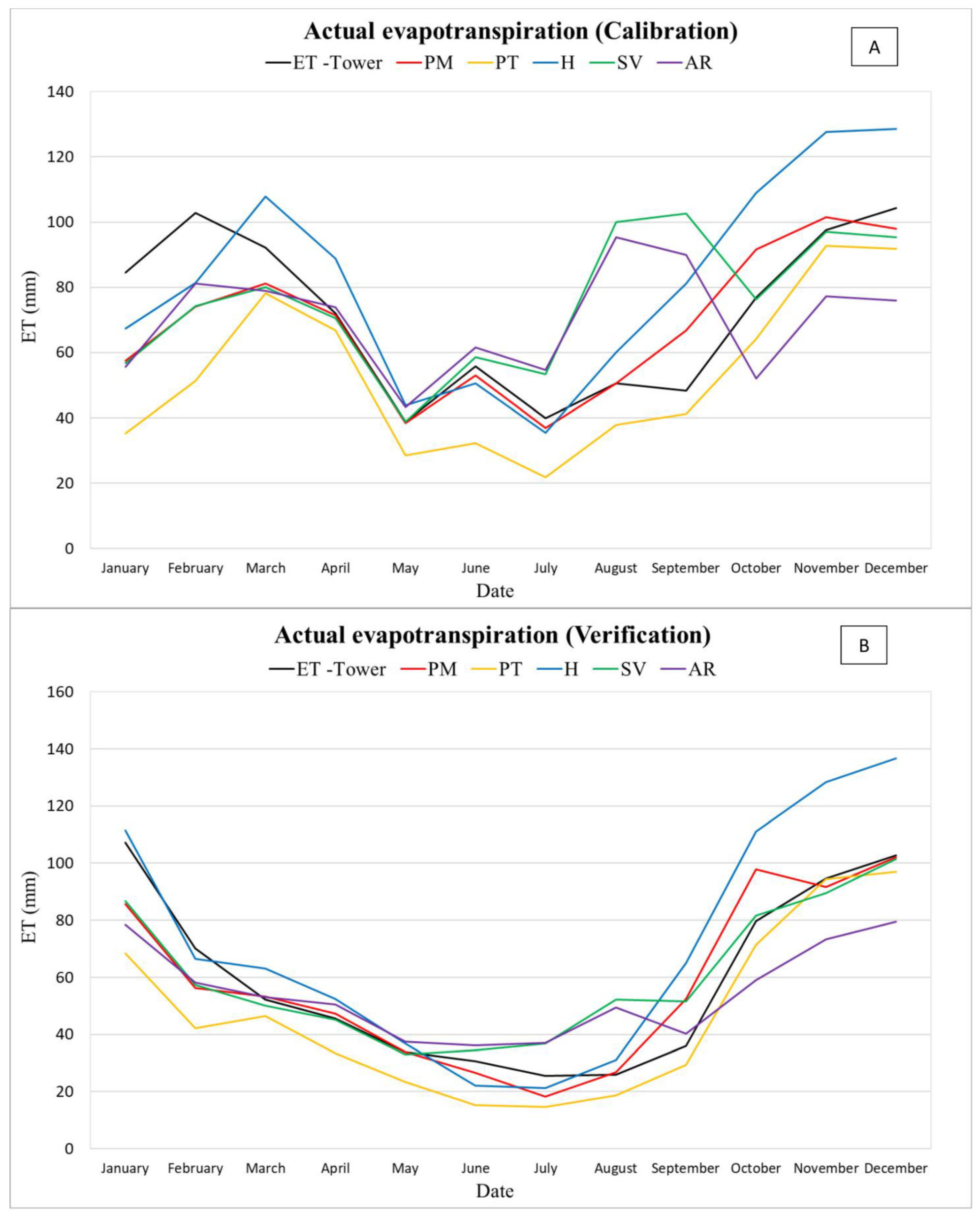
The comparison of actual evapotranspiration simulated in SWAT (ETsim) with ET values obtained by EC (ETobs) (

Table 4. Statistical coefficients obtained between actual evapotranspiration data obtained by EC and data simulated with the SWAT model obtained using the evaluated methodologies.

Stat. Coef.	Seas.	Period	PM	PT	H	SV	AR
MAE (mm)	Diary	Calibration	0.77	1.05	0.94	1.04	1.02
		Verification	1.01	1.03	1.02	0.89	0.89
	Rainy	Calibration	13.26	21.44	22.49	11.47	19.91
		Verification	8.53	14.16	17.78	6.3	16
	Dry	Calibration	4.94	14.34	11.42	24.03	22.32
		Verification	5.75	10.19	9.94	11.56	9.73
RMSE (mm)	Diary	Calibration	1.16	1.37	1.21	1.37	1.34
		Verification	1.45	1.26	1.34	1.17	1.16
	Rainy	Calibration	16.76	28.4	23.3	16.14	21.8
		Verification	11.97	19.2	22.25	9.41	18.63
	Dry	Calibration	8.51	15.48	15.79	33.44	28.32
		Verification	8.25	10.66	13.89	14.63	12.25
R	Diary	Calibration	0.46	0.47	0.5	0.19	0.18
		Verification	0.38	0.48	0.51	0.34	0.33
	Rainy	Calibration	0.39	0.37	0.37	0.58	0.61
		Verification	0.86	0.84	0.91	0.94	0.97
	Dry	Calibration	0.67	0.62	0.48	0.51	0.57
		Verification	0.87	0.82	0.77	0.11	0.35

) was performed for the five methodologies evaluated in this study. The analysis on a daily scale showed that, in general, there is similarity between the values, the MAE of all methods have values of up to 1.05 mm, the RMSE presented values between 1.16 mm and 1.45 mm, while R was the one that showed lower results with values from 0.18 to 0.51. On a monthly scale, among the evaluated methodologies, the rainy season (October to April) was the one with the greatest discrepancy between simulated and observed values. Regarding R, the AR and SV methods showed the worst adherence. In addition to the analysis of statistical coefficients, to assess the behavior of the ET, comparative graphs were plotted between the ETsim and monthly ETobs data for all methodologies evaluated in the calibration period (Figure 5A) and verification period (Figure 5B).

Among the PET methods investigated, Penman–Monteith was the most consistent method, with ETsim showing good agreement with the observed values. The highest similarity with ETobs was observed for the dry period. The Penman–Monteith method is the most applied globally [42,43,44,45,46], but this method requires a large amount of input data, which is not always available on a daily basis and with all of the required meteorological variables [3,21,47,48].

The Priestley–Taylor method, in general, led to underestimated values, despite statistically presenting adherence to the observed data; in monthly time steps, it is observed that in the rainy season the PT method presents better adherence to the observed data in comparison to the other methodologies. Vourlitis et al. [49] noted that the constant present in the PT formula for the tropics does not represent the seasonal behavior of the PET data. However, in the application of the SWAT model (Figure 5A,B) an underestimation was obtained, but the method follows the observed data in terms of seasonality.

The use of the simplified potential evapotranspiration method, the Hargreaves method, which has temperature as the only variable needed for simulation, allowed SWAT to generate statistically similar results to more sophisticated methods [22,50,51]. Graphically, on a monthly scale, the H method presents an overestimation of ETobs, mainly in the rainy period. In the recession periods, on the other hand, the method led to simulations more that were adherent to the ET values obtained by EC. This leads to the hypothesis of Oudin et al. [21] that potential evapotranspiration approaches based on Penman, which requires more variables to estimate evapotranspiration, seem less advantageous for feeding rainfall–runoff models.

Strauch and Volk [18] compared the SWAT output data at the HRU level with the average MODIS (NASA’s MODerate Resolution Imaging Spectro-radiometer) data for ET in the Cerrado and found good agreement between the data. However, the authors showed, by considering other works that contain MODIS data for ET in the Cerrado, that the data may be underestimated during the dry season but stated that the seasonal patterns were well reflected. In this research, it was noted that the ETsim values can well represent the monthly and annual behavior of ETobs. However, in the dry season, they present overestimates in some months. The SV method implemented a logistic function that considers a minimum LAI that should be seen as a general improvement, regardless of whether the study area is in the tropics or not. Furthermore, a sigmoidal (instead of linear) decline in LAI can also be considered more realistic for annual plants.

Arroio Junior [23] developed a modified version of SWAT and applied it to watersheds in the state of São Paulo that encompass agricultural areas. In this work, the method led to an underestimation in the rainy period, and an overestimation in the dry period. In general, compared to other methodologies, it presented a positive performance for the basin under study, although it is also similar to the PM method, which can lead to questions about the effort required for its application.

4. Conclusions

The SWAT model has been widely used to simulate agricultural areas. In this study, we analyzed the actual evapotranspiration of a pristine Brazilian Cerrado vegetation biome, comparing simulated values to the values estimated by turbulent flow EC tower data.

The calibration and verification, in terms of daily flows, using the five ET methods led to fair performance. The actual evapotranspiration obtained by EC (ETobs) compared to actual evapotranspiration simulated with SWAT (ETsim), using the PM, PT, H, SV and AR methods, highlighted SWAT’s potential to represent the actual evapotranspiration, proving that even with a calibration performed in terms of flow, the adjustment is adequate for the actual evapotranspiration process when compared to observed data. The Penman–Monteith and Hargreaves method led to better results for the dry season, and, for the rainy season, they overestimated the ET in relation to the observed data. In general, it was observed that all methods did not perform well for the rainy season.

The evaluation of the modifications proposed by Strauch and Volk [18], and by Arroio Junior [23], showed that, for an area predominantly occupied by Cerrado, no improvement in results was obtained in relation to the PM method. The modifications introduced complexity without this being reflected in a better representation of the phenomenon, as observed for the months in which the modifications are activated by the humidity conditions, in which the simulations showed divergent behavior from the observed values and those simulated by the default SWAT methods.

References

- Brutsaert, W. Hydrology–An Introduction; Cambridge University Press: Cambridge, UK, 2005. [Google Scholar]
- Morton, F.I. Operational estimates of areal evapotranspiration and their significance to the science and practice of hydrology. J. Hydrol. 1983, 66, 1–76. [Google Scholar] [CrossRef]
- Carvalho, T.; Reis, D.S., Jr. Avaliação da Influência dos Dados de Evapotranspiração Potencial no Desempenho de Modelos Hidrológicos em Bacias do Semiárido Cearense. In Proceedings of the IX Northeast Water Resources Symposium, Brazil, November 2008; Available online: https://scholar.google.com.br/citations?view_op=view_citation&hl=pt-BR&user=6K4NyGwAAAAJ&citation_for_view=6K4NyGwAAAAJ:3fE2CSJIrl8C (accessed on 23 July 2021).
- Bonumá, N.B.; Rossi, C.G.; Arnold, J.G.; Reichert, J.M.; Paiva, E.M.C.D. Hydrology evaluation of the Soil and Water Assessment Tool considering measurement uncertainty for a small watershed in Southern Brazil. Appl. Eng. Agric. 2013, 29, 189–200. [Google Scholar] [CrossRef]
- Amatya, D.M.; Irmak, S.; Gowda, P.; Sun, G.; Nettles, J.E.; Douglas-Mankin, K.R. Ecosystem evapotranspiration: Challenges in measurements, estimates, and modeling. Trans. ASABE 2016, 59, 555–560. [Google Scholar] [CrossRef]
- Calder, I.R.; Harding, R.J.; Rosier, P.T.W. An Objective Assessment of Soil- Moisture Deficit Models. J. Hydrol. 1983, 60, 329–355. [Google Scholar] [CrossRef]
- Zhang, L.; Walker, G.R.; Dawes, W. Predicting the effect of vegetation changes on catchment average water balance. In Cooperative Research Centre for Catchment Hydrology; CSIRO Land and Water, 1999; Available online: https://ewater.org.au/archive/crcch/archive/pubs/pdfs/technical199912.pdf (accessed on 23 July 2021).
- Pereira, D.D.R.; Martinez, M.A.; Pruski, F.F.; Silva, D.D. Hydrological simulation in a basin of typical tropical climate and soil using the SWAT model part I: Calibration and validation tests. J. Hydrol. Reg. Stud. 2016, 7, 14–37. [Google Scholar] [CrossRef] [Green Version]
- Kirchner, J.W. Getting the Right Answers for the Right Reasons: Linking Measurements, Analyses, and Models to Advance the Science of Hydrology. Water Resour. Res. 2006, 42. [Google Scholar] [CrossRef]
- Klemes, V. Dilettantism in Hydrology: Transition or Destiny? Water Resour. Res. 1986, 22, 177S–188S. [Google Scholar] [CrossRef]
- Beven, K.J. Prophecy, Reality and Uncertainty in Distributed Hydrological Modelling. Adv. Water Resour. 1993, 16, 41–51. [Google Scholar] [CrossRef]
- Monteith, J.L. Evaporation and environment. In Symposium of the Society for Experimental Biology; XIX, Swansea. The State and Movement of Water in Living Organisms. New York; Cambridge University Press: Cambridge, UK, 1965; pp. 205–234. [Google Scholar]
- Priestley, C.H.B.; Taylor, R.J. On the assessment of surface heat flux and evaporation using large-scale parameters. Mon. Weather Rev. 1972, 100, 81–92. [Google Scholar] [CrossRef]
- Hargreaves, G.H.; Hargreaves, G.L.; Riley, J.P. Agricultural benefits for Senegal River Basin. J. Irrig. Drain. Eng. 1985, 111, 113–124. [Google Scholar] [CrossRef]
- Arnold, J.G.; Moriasi, D.N.; Gassman, P.W.; Abbaspour, K.C.; White, M.J.; Srinivasan, R.; Santhi, C.; Harmel, R.D.; Van Griensven, A.; Van Liew, M.W.; et al. SWAT: Model Use, Calibration, and Validation. Trans. ASABE 2012, 55, 1491–1508. [Google Scholar] [CrossRef]
- Garbossa, L.H.P.; Vasconcelos, L.R.C.; Lapa, K.R.; Blainski, E.; Pinheiro, A. The use and results of the Soil and Water Assessment Tool in Brazil: A review from 1999 until 2010. In Proceedings of the 2011 International SWAT Conference & Workshops, Toledo, Spain, 15–17 June 2011. [Google Scholar]
- Bressiani, D.; Gassman, P.W.; Fernandes, J.G.; Garbossa, L.H.P.; Srinivasan, R.; Bonumá, N.B.; Mendiondo, E.M. A review of Soil and Water Assessment Tool (SWAT) applications in Brazil: Challenges and prospects. Int. J. Agric. Biol. Eng. 2015, 8, 9–35. [Google Scholar] [CrossRef]
- Strauch, M.; Volk, M. SWAT plant growth modification for improved modeling of perennial vegetation in the tropics. Ecol. Model. 2013, 269, 98–112. [Google Scholar] [CrossRef]
- Melo Neto, J.O. Análise de Sensibilidade Escalar do Modelo Hidrológico SWAT. Master’s Thesis, Federal University of Lavras, Lavras, Brazil, 2012. [Google Scholar]
- Castro, K.B. Avaliação do Modelo SWAT na Simulação da Vazão em Bacia Agrícola do Cerrado Intensamente Monitorada. Master’s Thesis, University of Brasília, Brasília, Brazil, 2013. [Google Scholar]
- Oudin, L.; Hervieu, F.; Michel, C.; Perrin, C.; Andréassian, V.; Anctil, F.; Loumagne, C. Which potential evapotranspiration input for a lumped rainfall–runoff model? Part 2—Towards a simple and efficient potential evapotranspiration model for rainfall–runoff modelling. J. Hydrol. 2005, 303, 290–306. [Google Scholar] [CrossRef]
- Kannan, N.; Santhi, C.; Williams, J.R.; Arnold, J.G. Development of a continuous soil moisture accounting procedure for curve number methodology and its behaviour with different evapotranspiration methods. Hydrol. Process. Int. J. 2008, 22, 2114–2121. [Google Scholar] [CrossRef]
- Arroio Junior, P.P. Aprimoramento das Rotinas e Parâmetros dos Processos Hidrológicos do Modelo Computacional Soil and Water Assessment Tool-SWAT. Ph.D. Thesis, University of São Paulo, São Paulo, Brazil, 2016. [Google Scholar]
- Maia, J.M.F.; Baptista, G.M.M. Clima. In Águas Emendadas; Fonseca, F.O., Ed.; Secretaria of Urban Development and Environment: Brasília, Brazil, 2008. [Google Scholar]
- Neitsch, S.L.; Arnold, J.G.; Kiniry, J.R.; Williams, J.R. Soil and Water Assessment Tool-Theoretical Documentation Version 2005; Blackland Research Center, Texas Agricultural Experiment Station: Temple, TX, USA, 2005; p. 541. [Google Scholar]
- Neitsch, S.L.; Arnold, J.G.; Kiniry, J.R.; Williams, J.R. Soil and Water Assessment Tool-Theoretical Documentation Version 2009; Blackland Research Center, Texas Agricultural Experiment Station: Temple, TX, USA, 2011; p. 654. [Google Scholar]
- Ritchie, J.T. Model for predicting evaporation from a row crop with incomplete cover. Water Resour. Res. 1972, 8, 1204–1213. [Google Scholar] [CrossRef] [Green Version]
- Brutsaert, W.; Stricker, H. An Advective-aridity Approach to Estimate Actual Regional Evaporation. Water Resour. Res. 1979, 15, 443–450. [Google Scholar] [CrossRef]
- Williams, J.R.; Jones, C.A.; Dyke, P.T. A modeling approach to determining the relationship between erosion and soil productivity. Trans. ASAE 1984, 27, 129–144. [Google Scholar] [CrossRef]
- Williams, J.R.; Jones, C.A.; Kiniry, J.R.; Spanel, D.A. The EPIC crop growth model. Trans. ASAE 1989, 32, 497–511. [Google Scholar] [CrossRef]
- Gassman, P.W.; Williams, J.R.; Benson, V.W.; Izaurralde, R.C.; Hauck, L.M.; Jones, C.A.; Atwood, J.D.; Kiniry, J.R.; Flowers, J.D. Historical Development and Applications of the EPIC and APEX Models. In Proceedings of the 2004 American Society of Agricultural and Biological Engineers (ASAE) Annual Meeting, Ottawa, ON, Canada, 1–4 August 2004. [Google Scholar] [CrossRef] [Green Version]
- Nunes, G. Aplicação do Modelo SWAT no Estudo Hidrológico e de Qualidade de Água da Bacia Hidrográfica do Lago Paranoá-DF. Master’s Thesis, University of Brasília, Brasília, Brazil, 2016. [Google Scholar]
- Reatto, A.; Martins, E.S.; Cardoso, E.A.; Spera, S.T.; Carvalho, O.A.C.J.; Silva, A.V.E.; Farias, M.F.R. Levantamento de Reconhecimento de Solos de Alta Intensidade do Alto Curso do Rio Descoberto, DF/GO, Escala 1:100000; Research and Development Bulletin: Distrito Federal, Brazil, 2004. [Google Scholar]
- Távora, B.E. Zona Ripária de Cerrado: Processos Hidrossedimentológicos. Ph.D. Thesis, University of Brasília, Brasília, Brazil, 2017. [Google Scholar]
- Sarmento, L. Análise de Incertezas e Avaliação dos Fatores Influentes no Desempenho de Modelos de Simulação de Bacias Hidrográficas. Ph.D. Thesis, University of Brasília, Brasília, Brazil, 2010. [Google Scholar]
- Ferrigo, S.; Minoti, R.T.; Koide, S. Utilização do modelo SWAT (Soil andWater Assessment Tool) na estimativa de produção de sedimentos decorrentes de diferentes cenários de uso do solo na bacia do córrego Capão Comprido no Distrito Federal. In Proceedings of the XIX Brazilian Symposium on Water Resources, Maceió, Brazil, November 2011; Available online: https://www.researchgate.net/publication/260422891_AVALIACAO_DA_UTILIZACAO_DE_DIFERENTES_METODOS_NA_CALIBRACAO_AUTOMATICA_DO_MODELO_SWAT (accessed on 23 July 2021).
- Ferrigo, S.; Minoti, R.T.; Koide, S. Análise do modelo SWAT na simulação de produção de sedimentos quando calibrado unicamente para a vazão em uma pequena bacia hidrográfica rural. In Proceedings of the X National Sediment Engineering Meeting, Foz do Iguaçu, Brazil, 5 December 2012. [Google Scholar]
- Ferrigo, S.; Minoti, R.; Roig, H.; Koide, S. Avaliação da utilização de diferentes métodos na calibração automática do modelo SWAT. In Proceedings of the XX Brazilian Symposium on Water Resources, Bento Gonçalves, Brasil, November 2013; Available online: https://www.researchgate.net/publication/260422891_AVALIACAO_DA_UTILIZACAO_DE_DIFERENTES_METODOS_NA_CALIBRACAO_AUTOMATICA_DO_MODELO_SWAT (accessed on 23 July 2021).
- Ferrigo, S. Análise de Consistência dos Parâmetros do Modelo SWAT Obtidos por Calibração Automática–Estudo de Caso da Bacia do Lago Descoberto–DF. Master’s Thesis, University of Brasília, Brasília, Brazil, 2014. [Google Scholar]
- Salles, L.A. Calibração e Validação do Modelo SWAT para a Predição de Vazões na Bacia do Ribeirão Pipiripau. Master’s Thesis, University of Brasília, Brasília, Brazil, 2012. [Google Scholar]
- Krause, P.; Boyle, D.P.; Bäse, F. Comparison of different efficiency criteria for hydrological model assessment. Adv. Geosci. 2005, 5, 89–97. [Google Scholar] [CrossRef] [Green Version]
- Gong, L.; Xu, C.; Chen, D.; Halldin, S.; Chen, Y.D. Sensitivity of the Penman–Monteith reference evapotranspiration to key climatic variables in the Changjiang (Yangtze River) basin. J. Hydrol. 2006, 329, 620–629. [Google Scholar] [CrossRef]
- Sharifi, A.; Dinpashoh, Y. Sensitivity analysis of the Penman-Monteith reference crop evapotranspiration to climatic variables in Iran. Water Resour. Manag. 2014, 28, 5465–5476. [Google Scholar] [CrossRef]
- Dinpashoh, Y.; Jhajharia, D.; Fakheri-Fard, A.; Singh, V.P.; Kahya, E. Trends in reference crop evapotranspiration over Iran. J. Hydrol. 2011, 399, 422–433. [Google Scholar] [CrossRef]
- Droogers, P.; Allen, R.G. Estimating reference evapotranspiration under inaccurate data conditions. Irrig. Drain. Syst. Eng. 2002, 16, 33–45. [Google Scholar] [CrossRef]
- Shiri, J. Improving the performance of the mass transfer-based reference evapotranspiration estimation approaches through a coupled wavelet-random forest methodology. J. Hydrol. 2018, 561, 737–750. [Google Scholar] [CrossRef]
- Andréassian, V.; Perrin, C.; Michel, C. Impact of Imperfect Evapotranspiration Knowledge on the Efficiency and Parameters of Watershed Models. J. Hydrol. 2004, 286, 19–35. [Google Scholar] [CrossRef]
- Kelleher, C.A.; Shaw, S.B. Is ET often oversimplified in hydrologic models? Using long records to elucidate unaccounted for controls on ET. J. Hydrol. 2018, 557, 160–172. [Google Scholar] [CrossRef]
- Vourlitis, G.L.; de Souza Nogueira, J.; de Almeida Lobo, F.; Pinto, O.B. Variations in evapotranspiration and climate for an Amazonian semi-deciduous forest over seasonal, annual, and El Niño cycles. Int. J. Biometeorol. 2015, 59, 217–230. [Google Scholar] [CrossRef] [PubMed]
- Wang, X.; Melesse, A.M.; Yang, W. Influences of potential evapotranspiration estimation methods on SWAT’s hydrologic simulation in a northwestern Minnesota watershed. Trans. ASABE 2006, 49, 1755–1771. [Google Scholar] [CrossRef]
- Chen, M.; Gassman, P.W.; Srinivasan, R.; Cui, Y.; Arritt, R. Analysis of alternative climate datasets and evapotranspiration methods for the Upper Mississippi River Basin using SWAT within HAWQS. Sci. Total. Environ. 2020, 720, 137562. [Google Scholar] [CrossRef]
Figure 1.
Study area location map.
Figure 2.
(A) Digital Elevation Model (DEM); (B) slope classes; (C) pedology; (D) land use and land cover in the Ribeirão do Gama Basin; (E) HRUs obtained for the study area, with emphasis on the HRU where the EC tower is located.
Figure 3.
Observed and simulated hydrographs in the calibration period (2013 to 2015) and the verification period (2016 to 2017): (A) PM method; (B) SV method with application of PM parameters; (C) AR method with application of PM parameters.
Figure 4.
Observed and simulated hydrographs in the calibration period (2013 to 2015) and the verification period (2016 to 2017): (A) SV method; (B) AR method.
Figure 5.
Comparison of the average monthly total actual evapotranspiration for the (A) calibration period and (B) verification period.