Sediment Transport and Water Flow Resistance in Alluvial River Channels: Modified Model of Transport of Non-Uniform Grain-Size Sediments

Abstract

The paper presents recommendations for using the results obtained in sediment transport simulation and modeling of channel deformations in rivers. This work relates to the issues of empirical modeling of the water flow characteristics in natural riverbeds with a movable bottom (alluvial channels) which are extremely complex. The study shows that in the simulation of sediment transport and calculation of channel deformations in the rivers, it is expedient to use the calculation dependences of Chézy’s coefficient for assessing the roughness of the bottom sediment mixture, or the dependences of the form based on the field investigation data. Three models are most commonly used and based on the original formulas of Meyer-Peter and Müller (1948), Einstein (1950) and van Rijn (1984). This work deals with assessing the hydraulic resistance of the channel and improving the river sediment transport model in a simulation of riverbed transformation on the basis of previous research to verify it based on 296 field measurements on the Central-East European lowland rivers. The performed test calculations show that the modified van Rijn formula gives the best results from all the considered variants.

1. Introduction

The problem of forecasting channel transformations in riverbeds with a movable bottom (alluvial channels) is one of the most complex in fluvial hydraulics [1]. Along with traditional research techniques, the methods of mathematical modeling have been and continue to be widely used in the modern practice of hydraulic calculations. In actual practice, the task is to perform hydraulic calculations of the water flow characteristics and sediment transport parameters (bottom deformations) in rivers. In terms of calculation, this boils down to solving by numerical methods a known set of equations of water movement, continuity and deformations at the given initial and boundary conditions. This set of equations in five unknowns is closed by two additional calculation dependences—the hydraulic resistance law in the form of Chézy’s formula and sediment discharge formula. Therefore, the quality of channel predictions largely depends on reliability of the energy loss estimates over the length and sediment transport parameters in the deformable channel.

1.1. Hydraulic Resistance Factors to Water Flow in Rivers

Hydraulic resistance of natural channels is one of the biggest challenges of river flow dynamics. The current level of this discipline [2] requires treating the river flow and movable channel as a single system, the interaction of which is based on the principle of feedback (flow $\leftrightarrow$ channel). As this takes place, the flow itself creates and regulates the roughness of its bottom. The complexity and lack of knowledge of this issue significantly limits the theoretical approach to its solution. Therefore, the results obtained in recent years are mainly empirical or semi-empirical. In the practice of engineering calculations, either hydraulic friction coefficient $\lambda$, or Chézy’s formula $C=\sqrt{2g/\lambda }$ are used.

The values of Chézy’s coefficient for natural channels are usually derived from the Manning formula [3], i.e., via dimension roughness factor n. Factor n expresses the cumulative effect of all resistances found in the natural channel, and therefore varies considerably. When dealing with long estimated areas, with resistance variations smoothed along their length, it is permissible to use the n values from tables of hydraulic reference guides. When performing calculations on relatively short distances, the use of tabulated values of the roughness coefficients is unacceptable. In this case, n is determined from the measurements of water discharge and slope, which, in turn, requires observations on the survey plot.

In determining the hydraulic resistance in a channel with sandy bottom sediments, another challenge is the relation of its value with the flow rate. Therefore, the use of the Manning formula or similar formulas with tabulated values of the roughness coefficient can result in gross errors for the movable channel.

As for the open channel, Meyer-Peter and Müller (hereafter MPM) suggested presenting the friction slope as the sum of the slope due to grain roughness of the bottom and the slope caused by the bed forms resistance [4]:

$$I=I_d+I_r$$

(1)

where I_d is the slope due to grain roughness of the bottom, I_r is the slope caused by the bed forms resistance.

Equation (1) corresponds to a known relationship between the Chézy coefficients [3]:

$$1/C^2=1/{(C_d)}^2+1/{(C_r)}^2$$

(2)

The contribution of each component of the Chézy coefficient $C_d$ and $C_r$ may be different in the different rivers depending on the size of the particles forming the bottom. In rivers with a sand channel, the main part of the lengthwise energy loss is due to the bed form resistance. Research results given by Grishanin [5] show that in the range of values of Chézy’s coefficient C < 50 m^1/2/s, which applies to most of the plain rivers with sandy bottom sediments, over 90% of the lengthwise energy loss is due to resistance of the bed form bottom relief.

The situation is different with resistance of the channels composed of coarse sediment. Its value in rivers with gravel and pebble bottom sediments is mainly determined by the grain roughness of the bottom. It depends on the size of the particles of the bottom material, represented as the H/d parameter, where H (m) is mean depth in river cross-section = ω/B; ω (m²) is cross-sectional area; B (m) is cross-section width; d (m) is median sediment diameter.

1.2. Grain Roughness

To estimate the grain roughness, the power formulas with the structure of Manning–Strickler [6] dependence and logarithmic formulas by the type of Zegzhda formula [7] are usually used in the engineering calculations. The Manning–Strickler empirical calculation dependence reads as:

$$C_d/\sqrt{g}=6.67{(R/d_{50})}^{1/6}$$

(3)

where C_d (m^1/2/s) is Chézy’s coefficient due to grain roughness, g (m/s²) the gravity acceleration, R (m) is hydraulic radius, and d₅₀ (m) is the value of the particle diameter at 50% in the cumulative distribution.

Through experiments in the open trays with pasted roughness, Zegzhda [7] obtained the calculation dependence reads as:

$$C_d/\sqrt{g}=5.66lg(R/D)+6.01$$

(4)

where g (m/s²) the gravity acceleration, R (m) is hydraulic radius, and D (m) is the height of the roughness protrusions, taken, respectively, equal to D = 1.6d₅₀ for sandy particles, D = 1.3d₅₀ for fine gravel particles, and D = d₅₀ for medium and coarse gravel.

The pebble riverbed resistance study was carried out by Griffiths [8]. The initial data in his study were 136 measurements at 72 reaches of 46 New Zealand rivers. Taking into account measurement data of some other authors (a total of 186 points), Griffiths obtained the resistance formula for a channel with an immovable bed:

$$C_d/\sqrt{g}=5.60lg(R/d_{50})+2.15$$

(5)

The analysis of research published on this work shows that the formula of form (4) has been extensively verified based on the field measurements and laboratory data and is recommended for use in calculations by a number of other authors [9,10,11,12,13,14]. These results indicate the increasing hydraulic resistance when passing from experiments in the trays to the river original flows. This becomes evident in the fact that all the authors have obtained different intersection values in Formula (4) for the constant term K. They vary from K = 6.01 of Zegzhda by measurements in trays with the attached sand roughness [7], and K = 2.15 [8] by Griffith’s Formula (5) to K = −5.3 of Grishanin [14] by measurements in the rivers with a pebble-boulder bed. Such significant variations in the values of the constant term K of different authors are due to the heterogeneity of sediment of the bottom sediments and additional resistance factors in the natural channel flows.

The first component of additional energy losses can be considered to some extent due to a more detailed evaluation of the distribution of the coarseness of granulometric composition when selecting the representative diameter of the bottom sediments. Ribberink [15] uses in his study the log normal particle size distribution law for the river alluvium. Considering the results of studies [16,17], the calculation expression for determining the representative diameter value d_a can be represented, which reads as:

$$d_a=1.6d_{50}{\sigma }_g^{-0.56}$$

(6)

where ${\sigma }_g=\exp \sqrt{ln\left[{(S_{dm}/d_m)}^2+1\right]}$ is the geometric standard deviation of the diameter logarithm from the mean by the value equal to the standard deviation; otherwise—${\sigma }_g=0.5\left[d_{84}/d_{50}+d_{50}/d_{16}\right]$, where $d_{84}$ and $d_{16}$ are characteristic particle diameters equal to the 84- and 16-percentile size, respectively.

$S_{dm}=\sqrt{\sum {\beta }_i{\left(d_i-d_m\right)}^2}$—standard deviation from the mean diameter; $d_m=\sum {\beta }_i{d}_i$—mean diameter of particles in the mixture; ${\beta }_i$—relative content of i fraction in sediment in the mixture, d_i—diameter of the i-th particle fraction in the mixture. These dependences can be used for river flows with smooth beds.

The impact on water flow resistance can also be associated with randomly distributed individual accumulations of coarse particles at the bottom of the river, as well as the presence of the bed forms. The latter may be a relict, and their sizes are uniquely unrelated to the flow characteristics. Therefore, it is not possible to use the available techniques to assess the contribution of the bed form component. In this case, the only possible solution is to use the empirical relation and try to link the grain roughness value with the value of the lengthwise total resistance. There were several such studies conducted by Griffiths [12], Kishi and Kuroki [18] and Engelund and Hansen [19], but only Griffiths used the materials of measurements for rivers with coarse-grained sediment. On the basis of experimental data of Jaeggi [20] and MPM, he derived the following design formula for tranquil flows:

$${\Theta }_r\equiv {\tau }_{*r}={\tau }_{*}-{\tau }_{*d}=exp(-b{\tau }_{*}{}^{-m})\cdot \left({\tau }_{*}-{\tau }_{*c}\right)$$

(7)

where b = 0.142 and m = 0.71 are regression coefficients respectively, ${\Theta }_r$ or τ_*r the dimensionless shear stress due to bed forms, τ_*d the dimensionless shear stress due to grains and τ_* the dimensionless shear stress due to both grain roughness and bed form roughness.

Given that additional resistance factors in the natural beds cannot be identified and evaluated as of today, the use of integral estimation based on the field measurements data allows for a sufficiently reliable description of the flow—channel interaction process in rivers with coarse-grained sediment.

1.3. Bed Forms Resistance—Total Lengthwise Resistance

The hydraulic resistance to water flow in rivers with fine-grained bottom sediments differs significantly from the resistance of pebble-gravel beds. The main differences are as follows.

In rivers with sandy bottoms, the share of grain roughness becomes much smaller. This is due to the relatively large values of H/d. Moreover, as shown by the results of studies, there is sediment sorting on the bed forms surface in sand beds. Therefore, the representative diameter of the bottom sediments on the pressure bed form slope is less than the value estimated for the original mixture.

The second difference is that the size of the bottom forms in the sand beds weakly depends on the change in coarseness of the bottom sediments.

Finally, due to the high mobility of the sand particles, the channel forms are transformed by the flow when water movement characteristics change. Therefore, the water flow of the river is able to regulate the roughness of its bottom in virtually the entire range of the runoff change during a calendar year.

Grishanin [14] derived the functional dependence of the formula below when exploring hydraulic resistance of quasi-uniform flows with a sand bed and developed bed form roughness (channel reaches in rectilinear reaches of the hollows):

$$C/\sqrt{g}=f\left(U/\sqrt[3]{g\nu },B/H\right)$$

(8)

where C (m^1/2/s) is Chézy coefficient related to the roughness due to grains and bed forms, U (m/s) is mean flow velocity, g (m/s²) acceleration of gravity, v (m²/s) is kinematic viscosity coefficient, B (m) the channel cross-section width, and H (m) is mean riverbed hydraulic depth in river cross-section.

When these scales were chosen as the main arguments for Chézy’s coefficient, it was taken into account that resistance of the flat bottom made up of the sand fraction particles is in principle affected by viscosity, while the variations of the particle diameter within the boundaries of this fraction has no detectable effect on either the resistance of the flat bottom, or on the bed form resistance.

The resulting design formula for total Chézy coefficient is written as:

$$C/\sqrt{g}=5.25{(U/\sqrt[3]{g\nu })}^{1/2}{(H/B)}^{1/6}$$

(9)

where Chézy coefficient related to the roughness, U is mean flow velocity, g acceleration of gravity, v is kinematic viscosity coefficient, B the channel cross-section width, and H is mean riverbed hydraulic depth in river cross-section.

Formula (9) was confirmed with a high correlation coefficient for field measurement data. The second argument in the formula is the dimensionless depth of the flow or the value reciprocal of the relative channel width. From the obtained relation it follows that with equal flow velocities, hydraulic resistance to water movement is less in relatively large and deep rivers than in small and broad ones. The second conclusion is that Chézy’s coefficient increases with increasing water levels in the river.

Gladkov [21], studying bed resistance at the ripples, suggested that it is associated with the kinetic energy of the flow. The main objectives of the author are based on the idea that ripple washout at low-water levels is more intense, the larger the slope of the free surface I, and in the course of washout, the average length of bed form $l_r$ increases. This suggests a proportionality relation $l_r/H$~I between the relative length of bed form $l_r/H$ and slope $I$.

To test the stated objectives, the materials of field measurements and the ripples of a number of navigable rivers were used, as well as data of the “Inland Waterways Map” at the reaches of several major navigable rivers of Russia. The sample size of the field measurement data amounted to 296 measurements at the time of the study. A new dependence of Chézy’s coefficient was obtained from these data:

$$C/\sqrt{g}=18.6{\left(\frac{U}{\sqrt{gH}}\right)}^{3/4}{\left(\sqrt[3]{\frac{g{H}^3}{{\nu }^2}}\right)}^{1/8}$$

(10)

The formula obtained is not inferior in accuracy to design Formula (9). The field of their possible application in practice should be linked with the dimension of the hydrodynamic model used in the calculations. Formula (9) can be recommended for solving problems in a one-dimensional definition, and the design formula of Form (10) in a two-dimensional definition, respectively. The possible field of their application is limited to the set of rivers with sandy bottom sediment at flow rates ensuring the transport of sediments in the type of the bed form.

Analysis of the results shows the changing nature of the relation between Chézy’s coefficient and determining factors at various morphological elements of the river channel. In reach hollows, water flow velocity represented in a dimensionless form is the main argument of water movement resistance, in quasi-uniform water movement in the rivers (9). The functional linkage with the B/H parameter in the resulting formula is weaker than with the flow velocity.

A different picture is observed in the ripples and shallow reach hollows at low water levels. The kinetic energy of the flow increases under these conditions, which leads to an increased linkage of Chézy’s coefficient to the flow depth. Both types of channel formations—ripples and reach hollows—can be found at river bends, and both types of dependences of Chézy’s coefficient can be implemented.

With the establishment of new dependences, the design practice has the description of the mechanism of interaction of the river flow and the movable bed. The resulting formulas of Chézy’s coefficient implicitly consider the changing parameters of the bed forms and lengthwise energy losses caused by them with a change in the boundary water movement conditions. The use of these formulas in hydraulic calculations enables assessing the effect of water transport engineering measures on the hydraulics of the river flow and sediment transport conditions in rivers.

Further improvement of the justifying calculations in the field of sediment transport is associated with objective difficulties. Until now, the assessment of the water resistance value and sediment flux in the river channel have been studied separately. However, the value of energy losses over the length, which is estimated by the Chézy formula, enters into the water movement equation and the deformations equation within the sediment flux formula. Therefore, when analyzing the sediment transport characteristics in rivers, it is difficult to find objective and physically measurable parameters of displacement of the river alluvium particle under the action of the flowing water.

The main objective of this study is to verify different sediment transport models on the basis of previous research and to verify them based on the measurements on the alluvial stretches of rivers and a modified model of transport of non-uniform grain-size sediments. Implementation of the works is to allow outlining further steps of improving sediment transport models for use in the design practice. To test the stated objectives, the materials of detailed measurements of a number of navigable lowland rivers were used, as well as data of the “Inland Waterways Map” at the reaches of several major navigable rivers of Central-Eastern Europe.

2. Materials and Methods

2.1. Input Data for Testing the Model

Various sediment transport formulas were tested in the study based on the data sample of measurements carried out on rivers with different coarseness of the bottom sediments. Materials of the measurement taken on the large and medium alluvial rivers of the lowlands, in the reaches of mountain and piedmont rivers with coarse-grained bottom sediments, as well as the materials of the two series of experimental lab studies in the scaled hydraulic flume with movable bottom [22] were used for sample design. At this stage, the input data sample includes measurement results on 41 hydraulic sections of 29 different rivers of Russian territory and several former USSR republics, published in the State Inventory of Water Resources [23], as well as measurements on other Central-Eastern European rivers [17]. General characteristics of the adapted data sample are presented in

Table 1. General characteristics of the sample of measurement materials for calibration of the sediment transport model. Adapted from: Danube and Isar [17], others [23].

River Name, Water Gauge Post and Country	Years of Measurements	Mean Water Velocity (m/s), From/To	Mean Channel Depth (m), From/To	Diameter of the Sediment Grains (mm), From/To	Water Surface Slope (‰), From/To	Number of Measurements
Danube (Pfelling, Hofkirchen—Germany)	1970, 1971 1989–1991	0.95/1.94	3.10/5.92	10.7/17.6	0.11/0.34	9
Isar (Plattling—Germany)	1988, 1989	1.44/2.12	1.48/2.61	22.5	0.85/0.89	3
Niekuchang (Russia)	1955	0.98/1.71	0.32/0.49	93.2	9.8/11	4
Burtochan (Russia)	1955	1.22/1.70	0.45/0.70	50.1	4.0/4.6	4
Chu (Tashkul Village—Kazakhstan)	1949, 1955	0.5/1.25	0.8/2.17	0.31/2.55	0.30/0.62	25
Desna (Chernigov—Ukraine)	1964, 1955	0.44/0.95	3.73/6.30	0.25/0.27	0.029/0.10	6
Moscow (Zvenigorod—Russia)	1952, 1955	0.29/1.06	0.39/3.68	1.63/1.76	0.16/0.38	16
Yenisei (Minusinsk—Russia)	1958	0.44/0.87	1.14/2.86	21.1	0.08/0.20	6
Klazma (Kovrov—Russia)	1950, 1951	0.40/1.10	3.83/6.2	0.59/2.12	0.027/0.078	13
Suda (Kurakino—Russia)	1949	0.40/0.98	1.84/2.72	3.49	0.086/0.21	10
Mologa (Ustyuzhna—Russia)	1951, 1952	0.31/0.81	1.08/3.96	1.83/2.48	0.036/0.13	13
Ob (Ogurtsovo—Russia)	1950, 1951	0.63/1.27	1.34/5.3	0.36/0.47	0.036/0.15	36
Volga (Yaroslav—Russia)	1953	0.59/0.77	6.0/7.0	0.99	0.035/0.045	3
Kara Darya (Uzbekistan)	1955–1958	1.29/2.77	0.81/1.95	39.6/56.8	2.1/4.1	25
Arys (Kazakhstan)	1957, 1955	0.46/0.87	0.39/2.99	1.72/3.66	0.28/0.63	15
Naryn (Kirghizia)	1955	1.37/2.08	2.55/3.43	47.6	0.86/1.6	12
Kurta—(Kazakhstan)	1956–1958	0.36/0.84	0.09/0.82	0.71/2.83	0.35/1.4	28
Dnieper (Kiev—Ukraine)	1959	0.39/0.78	2.96/7.0	0.34	0.041/0.065	8
Oka (Novinki—Russia)	1946	0.57/0.82	2.07/6.3	0.24	0.015/0.035	4
Charysh (Charyshsky Village—Russia)	1951	0.63/0.67	2.54/2.63	0.51	0.26/0.37	2
Togul (Togul Village—Russia)	1951	0.33/0.55	0.26/0.41	3.53	0.08/0.21	2
Burla (Habara Village—Russia)	1951	0.09	0.14	0.41	0.27	1
Ishim (Petropavlovsk—Kazakhstan)	1952	0.16/0.64	0.70/4.9	0.65	0.03/0.11	9
Chulyom (Communarca—Russia)	1952	0.88/1.07	5.4/5.7	0.7	0.09/0.092	3
Vyatka (Kirov—Russia)	1954	0.60/0.84	1.8/4.23	0.99	0.093/0.13	10
Suuremayygi (Kvissental—Estonia)	1956	0.27/0.64	3.27/4.5	4.1	0.022/0.088	9
Don (Kazan Village—Russia)	1953	0.62/1.00	5.4/7.3	0.27	0.041/0.095	7
Sheksna (Black Grow—Russia)	1949	0.23/0.56	3.97/4.97	0.37	0.003/0.022	10
Nura (Sergei Village—Kazakhstan)	1948	0.19/0.47	0.47/0.96	4.75	0.47/0.53	3
Overall outliers for the sample	-	0.09/2.77	0.09/7.3	0.25/93.2	0.003/11.0	-

.

All measurements published in the State Inventory of Water Resources [23] and data from the Federal Waterways Engineering and Research Institute (Bundesanstalt für Wasserbau) used by Söhngen [17] were carried out with grab samplers for collecting sediment samples from hard bottoms (sand, gravel) using a unified approved methodology by certified measuring instruments at stationary hydrological posts of the state networks. Hydraulic and morphometric characteristics within the sample vary over a rather wide range. Thus, the mean flow velocity values vary from 0.09 to 2.77 m/s; mean flow depth—from 0.09 to 7.3 m; diameter of the sediment grains—from 0.25 to 93.2 mm; free surface slopes—from 0.003 to 11.0‰, i.e., by 3660 times.

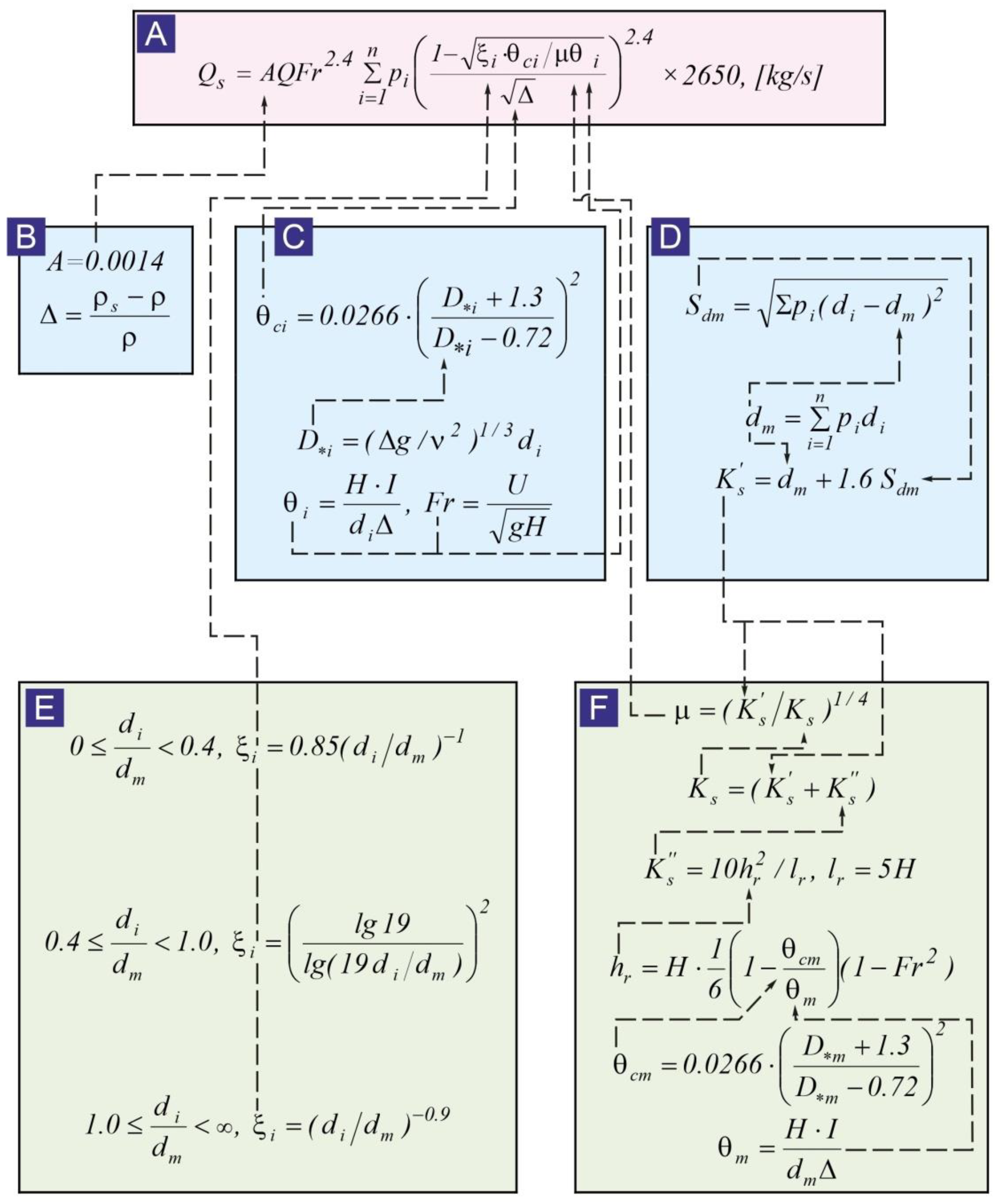
2.2. The Structure of the Transport Model for Non-Uniform Size of Grain Bottom Sediments

The design formulas of MPM [4], van Rijn [24,25], Hunziker [26,27], Parker [28,29] and Einstein [30] and their modifications (a total of 30 calculation models) were used as the main dependences for modeling the transport of non-uniform grain-size sediments for the purpose of their verification [31]. Ribberink models were used as known modifications of the formula of MPM [15] and the Federal Waterways Engineering and Research Institute (BAW) [17,32]. Calculations were also performed by the van Rijn formula modified by Lagucci [33]. A number of new modifications of these formulas have been plotted based on experimental and field measurement data obtained by the author’s research [21]. The calculation algorithm using the modified formula of van Rijn is presented in Figure 1. Test calculations were performed taking into account the mean diameter, and by fractions. The original formula of van Rijn [25] was derived from measurements of sediment discharge on large rivers Q_s (kg/s) and tested against 226 measurements. The range of particle diameters varied from 0.1 to 2.0 mm, depths from 1 to 20 m, and the flow velocity from 0.5 to 2.5 m/s. van Rijn’s formula is written as:

$$Q_s=0.005\cdot Q\cdot {\left(\frac{U-U_c}{\sqrt{\frac{{\rho }_s}{(\rho -1)gH}}}\right)}^{2.4}$$

(11)

where Q (m³/s) is volumetric flow rate, U (m/s) is mean flow velocity, U_c (m/s) the critical flow velocity, ρ_s (kg/m³) and ρ (kg/m³) are densities of particles and water respectively, g (m/s²) the acceleration of gravity, v (m²/s) is kinematic viscosity coefficient, B (m) the channel cross-section width, and H (m) is mean riverbed hydraulic depth in river cross-section.

The value of the critical velocity U_c for sand with a size of $0.5\le d_{50}<2.0$ mm in van Rijn’s formula is calculated according to the following relationship:

$$U_c=8.5d_{50}^{0.6} lg \left(\frac{12H}{6d_{50}}\right)$$

(12)

The modification of van Rijn’s formula shown in Figure 1 was obtained in [31]. In this work, this formula was tested on the basis of 296 measurements on rivers (Table 1). The improvement of van Rijn’s formula was achieved by solving the following issues. The developed sediment transport model uses a new expression (see Box C in Figure 1) to assess the stability conditions of sediment particles at the bottom, obtained on the basis of experimental data by Knoroz [22,34] for a wide range of grain size variation bottom sediments. The new model takes into account the effect of changing the critical conditions for the shear of particles of different-grained sediments in the mixture (see Box E on Figure 1)—the so-called Hiding-Exposure (HE) coefficient. The recommended calculation methodology is based on independent proven materials of theoretical and experimental studies carried out by Kishi and Kuroki [18], Egiazaroff [35] and Söhngen [32].

In Boxes D and F, based on the research results by Ribberink [15], an algorithm is shown for calculating the relative proportion of grain roughness, the so-called ripple factor in the form $\mu {\Theta }_i$. River channel parameters are calculated according to the recommendations by Yalin and Karahan [36].

During the calculations by each design formula, a regression dependence of the form $ln{(Q_s)}_{meas}=a+b\left(ln{(Q_s)}_{calc}\right)$ was plotted between the measured and calculated sediment transport rates, by which the correlation of that linkage was evaluated.

The second criterion for determining the quality of calculations by each model was the requirement to keep the author’s interpretation of the tested formula. The exponent at the flow velocity (mobility ratio) in the sediment discharge formula remains unchanged with the angular coefficient b = 1 in the regression equation.

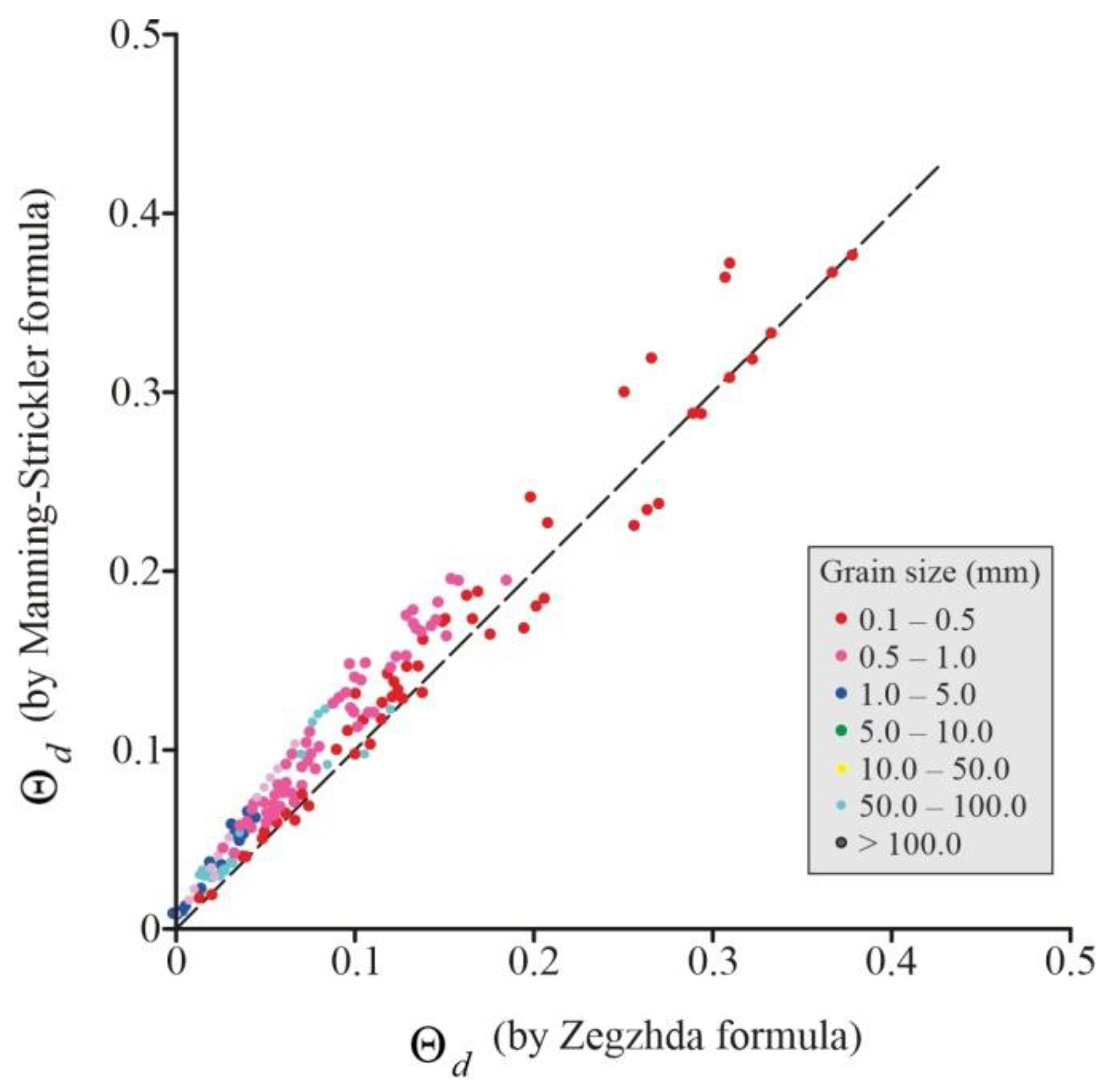
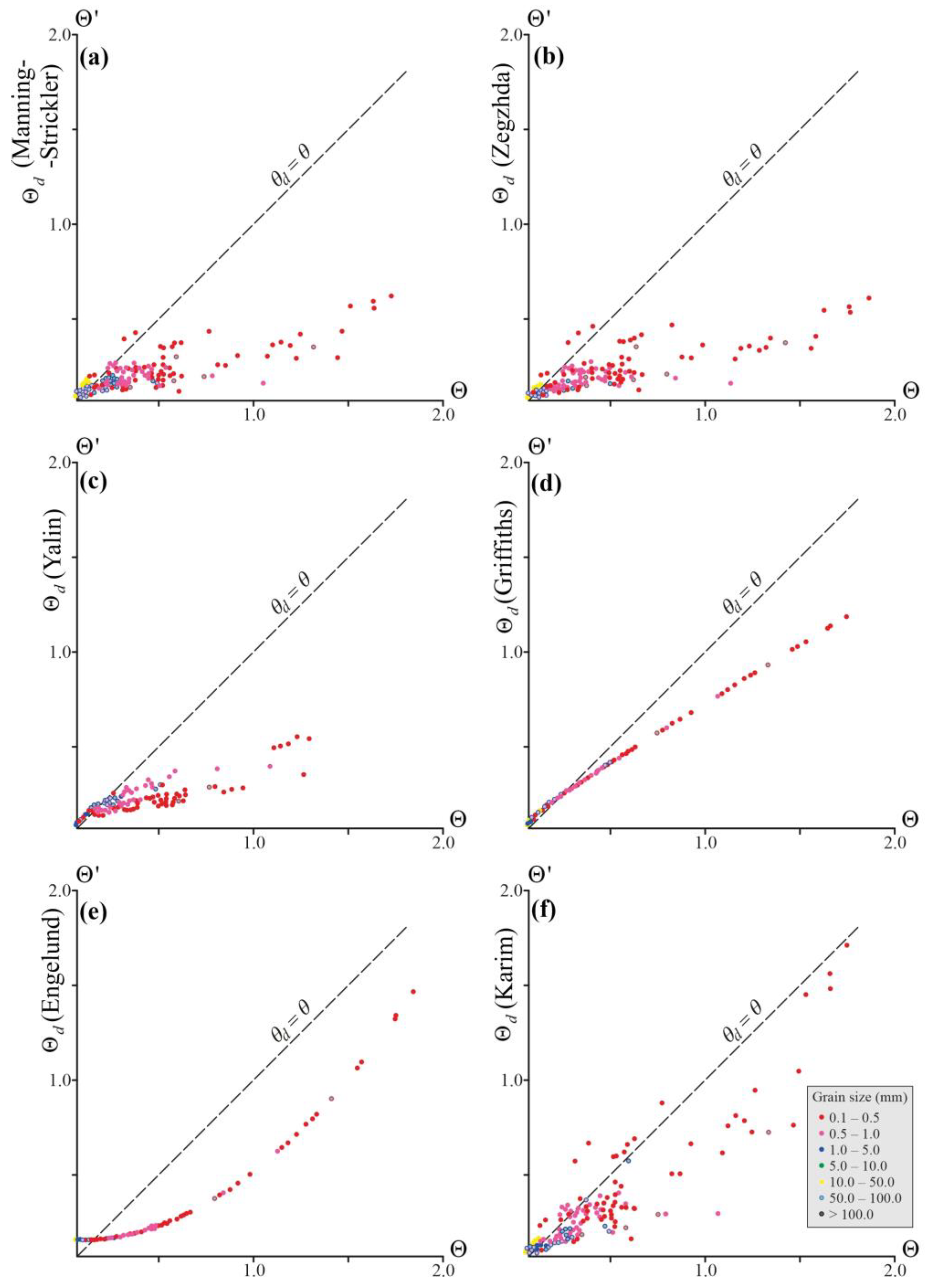
2.3. Test Calculations of the Grain Roughness Resistance in Natural Channels

Based on the available input data sample, various formulas for estimating the grain roughness resistance in natural channels have been tested. The design formulas of Manning–Strickler, Zegzhda [7], Griffiths [8], Yalin and Karahan [36], Engelund [37] and Karim [38] were used in the calculations. Given that each of the analyzed calculation dependences has empirical coefficients the values of which depend on the research conditions in each case, the work was carried out in two stages.

At the first stage, separate formulas for calculating grain roughness of the channel were compared with each other. This approach implies certain convention, because it is not possible to distinguish the relative proportion of the grain roughness alone, and it is unclear which of the analyzed formulas should be assumed as basic for comparison. In this regard, the second stage of calculations was carried out, in which the values of tractional sediments discharge were calculated using the modified sediment discharge van Rijn formula. In this work a solution was tested, according to which the value of the mobility coefficient corresponding to the relative fraction of the granular bottom roughness was calculated, which reads as: ${\Theta }_d=\mu \cdot \Theta$, where μ is ripple factor, $\Theta \equiv {\tau }_{*}=\frac{\rho {(U_{*})}^2}{\left({\rho }_s-\rho \right)gd}$ is mobility coefficient or dimensionless shear stress due to grain and bed form roughness, ${\Theta }_d$ is mobility coefficient (dimensionless shear stress) due to grain roughness, $U_{\ast }$(m/s) is bed shear velocity and d (m) grain diameter. In this work, a different scientific and methodological approach was adopted. The same modified formula of van Rijn was adopted as the basic formula for testing the sediment transport model, which showed relatively better results at the previous stages of research [31]. The main difference lies in the use of a different approach to estimate the value of the ripple factor (see Boxes D and F). The relative fraction of the granular roughness of the bottom was determined using the value of the Chézy coefficient $C_d$ calculated by the formulas of various authors (see Figure 2 and Figure 3). The value of the mobility coefficient corresponding to the granular roughness of the bottom was found using the well-known formula:

$${\Theta }_d\equiv {\tau }_{*d}=U_{*d}^2/\mathsf{\Delta }gd=U^2/C_d^2\Delta d$$

(13)

where $\mathsf{\Delta }=\frac{{\rho }_s-\rho }{\rho }$.

Checking the quality of the model was carried out as follows. According to the modified van Rijn formula shown in Figure 1, using an array of initial data (see Table 1), the values of sediment discharge were calculated. As mentioned above, when performing these calculations, the value of the mobility coefficient ${\Theta }_d$ corresponding to the granular roughness of the bottom was calculated using the Chézy coefficient according to the above, Formula (13). Accordingly, Boxes D and F shown in Figure 1 were not involved in the calculations in this case. Further, the calculated values of sediment flow rates were compared with the measured sediment discharges and thus the values of empirical coefficients in the used formulas of Chézy’s coefficient $C_d$ were finalized.

The formulas of Manning–Strickler and Zegzhda [7] of the mobility coefficient ${\Theta }_d$ were compared. This allowed for certainty in the assessment of the results obtained and outlining the next steps of research in this field. On the basis of the calculations made with the available input data sample (see Table 1), the ${\Theta }_d=f\left(\Theta \right)$ graphs were plotted. The ${\Theta }_d$ value in each case was calculated from the different formulas of Chézy’s coefficient for estimating the grain roughness of the bottom.

3. Results

3.1. Sediment Transport Model for Non-Uniform Size of Grain Bottom Sediments

The structure of the transport model for non-uniform grain-size sediments test calculations showed that of all the options considered, the best calculation results are obtained based on the original van Rijn formula [24,25], developed by the author for calculating the fine-grained sediment discharge in rivers [31]. In this work, we have made some headway. Calculations using the Manning–Strickler and Zegzhda formulas showed that when using the constant term, A = 0.001 in the calculation formula for the sediment discharge by van Rijn, the quality of calculating the sediment discharge becomes higher than that obtained at the previous stage of the study at A = 0.0014. Modification of this dependence enabled expanding the field of its possible use for a wider range of particle size of sediment of the bottom in rivers. At the same time, the calculations performed on the basis of the Strickler formula give the best results in the author’s interpretation of the formula. The value of the free term in the Zegzhda formula turned out to be 1.0, which coincides with the result obtained earlier by Limerinos.

Comparison of the calculated values of the tractional sediment discharges with the measurement data indicate their satisfactory coincidence. The correlation coefficient in the regression equation was 0.887. According to the model testing results, the angular coefficient b in the regression equation was 0.997, which allowed keeping unchanged the exponent value 2.4 as set by the author in the modified formula.

The performed calculations have shown the improved modeling quality when passing from the calculation by the mean diameter to calculation by fractions. This suggests that the guidelines used to account for the ripple factor and hiding effect are correct; models for accounting for them do not conflict with the general calculation procedure and are physically grounded. The calculation results are almost independent of the input data processing technique. They can equally use the arithmetic mean and geometric mean scores of the fractional composition.

The quality of sediment discharge calculation by the MPM formula in its author’s form and in its various modifications turned out to be lower than by the van Rijn formula. In all variants of the test calculations, the angular coefficient in the regression equation proved to be different from one (1.0), and was b = 0.77 on average. In this connection, the field of the possible use of the original dependence of MPM should be limited to the range of values of the large particle diameters, set by the authors in deriving it.

Finally, the probabilistic formula of Einstein [30] turned out to be rather satisfactory in terms of the accuracy of calculations. As for all other calculation dependences, test calculations showed relatively lower results compared with the field measurement data.

3.2. Sediment Mobility Coefficient Calculations

The factor that was not considered at this stage of research is associated with evaluating the hydraulic resistance of the channel. This is because the value of the mobility ratio (by Shields’ method) was calculated on the basis of measurements of the free surface slopes. In design practice, i.e., the free surface slope value is determined by calculation at each computation step when modeling the reformations in the river channel, depending on the calculated (set) value of Chézy’s coefficient. Therefore, it is not quite correct to talk about the quality of sediment transport model without solving this issue. These problems must be solved together, which was the subject of further research.

At this stage, an attempt is made to exclude the intermediate steps of computations associated with distinguishing the bed form component of energy losses over the length and to find the value of the mobility coefficient in the sediment discharge formula using Chézy’s coefficient by the known formula of grain roughness.

Given that quite a number of such formulas are used in the design practice, this study undertakes to test them and develops guidelines on improving the calculation procedure for the sediment transport parameters in rivers.

The data obtained from the comparison of formulas of Manning–Strickler and Zegzhda show that the mobility coefficient calculation results by these formulas match well with one another. In the range of small values of the mobility coefficient, i.e., for relatively larger particles, the Manning–Strickler formula gives higher values in the calculations compared with the Zegzhda formula. The results of the comparison of separate formulas for calculating grain roughness of the channel are shown in Figure 2. The formulas of Manning–Strickler and Zegzhda of the mobility coefficient ${\Theta }_d$ were compared.

Graphs were plotted on the basis of the calculations made with the available input data sample (Table 1). The value in each case was calculated from the different formulas of Chézy’s coefficient for estimating the grain roughness of the bottom. Comparison of the results of calculations is shown in Figure 3.

Analysis of the obtained results suggests the following conclusions. The closest results between themselves were received from the formulas of Manning–Strickler and Zegzhda (Figure 3a,b). The number of values that fell in the ${\Theta }_d\ge \Theta$ range, was smaller with the Zegzhda formula than with Strickler’s formula. This indicates that the design formula of Zegzhda will give more accurate calculation results in the range of small values of the mobility coefficient than the design formula of Strickler, with other things being equal.

The results of calculations performed using the Yalin and Karahan technique [36] correlate fairly well with the data obtained with the first two formulas; however, this technique also yields conservative values of ${\Theta }_d$ in the range of low mobility of the particles (Figure 3c). In calculating the bed form height by the Yalin and Karahan technique, an additional parameter—a critical value of mobility coefficient ${\Theta }_{cm}$—is used. In our case, its value was found from the calculation dependence based on the experimental studies of Knoroz [34].

Analytical dependence ${\Theta }_d=f\left(\Theta \right)$ established by Griffiths, judging on the data obtained, overstates the relative proportion of the grain roughness. This is most strongly manifested in the range of large values of the mobility factor, i.e., in relation to the small-size particles (Figure 3d). The ${\Theta }_d$ value calculated with this formula is significantly greater in virtually the entire range than the values obtained by the formulas of Shtrickler, Zegzhda and Yalin and Karahan. Apparently, the constant term value obtained by the author in the regression equation should be adjusted according to this calculation dependence when calculating the sediment discharge value.

Graph ${\Theta }_d=f\left(\Theta \right)$ based on calculations by the Engelund formula [37] has a reverse curvature in comparison with other analyzed formulas (Figure 3e). This is difficult for physical justification, and additional experimental and field measurement data should be further involved for test calculations to make a decision regarding the possible use of this formula in the calculations.

The graph obtained from calculations by the Karim formula [38] clearly shows the regions separating the mobility grade of small and relatively larger particles. This is apparently due to the fact that the author’s original formula was tested by measurements on rivers with fine-grained material. However, even for these fractions, the scatter of points on the graph was rather wide (Figure 3f).

To assess the accuracy of calculations of the tractional sediment discharge using the selected calculation dependences of energy losses over the length, the second stage of calculations was carried out in the study, in which the results of calculations were compared with field measurements on the rivers using the available sample. The following method was adopted for calculations.

The modified van Rijn formula was used as a basic model for testing the sediment transport rate; it is described in this figure. The test calculations were performed for all of the above formulas of Chézy’s coefficient. In the course of the calculations, the values of the parameter in the original formula were defined with all the above-described design formulas, allowing estimation of the grain roughness proportion in each case, and, if necessary, making the necessary adjustments of its value. The comparison of the calculation values of sediment transport rate with the measurements was used as an objective criterion of the performance quality of a particular design formula for estimating the grain roughness of the channel.

4. Discussion

The results obtained in the course of verification of different sediment transport models based on the field measurement data allowed outlining further steps of their improvement for use in the design practice. They are as follows in general terms. According to the carried-out analysis, it is further expedient to develop three main models based on the original formulas MPM [4], Einstein [30] and van Rijn [24,25], with an account of their possible modifications on the basis of the research by Ribberink [15], Knoroz [34] and Gladkov [39,40]. In such a combination, these models give better results when verified by field observations on the rivers in a wide variation range of hydraulic and morphometric parameters.

Despite certain progress in recent years was achieved through research into the energy loss valuation problem for natural channels with a movable bottom, there is still a number of unresolved issues. The main difficulty is that the stream flow interacting with a movable bottom independently regulates the boundary conditions of its movement through the degrees of freedom it has. In this case, the nature and direction of changes in the flow channel system are still not clearly understood [41].

With reference to the flows with deformable channels, the distribution of hydraulic resistance along the length depending on contributing factors such as grain roughness of the bottom, bed form resistance and channel form resistance, is quite difficult, as the contribution of each of the components varies both over the river length and depends on time, more specifically on the hydrological cycle. Therefore, the need for distinguishing the relative proportion of any type of water movement resistance is always a certain convention, and in each case depends on the problems to be solved. At the reaches of the rivers with movable sediments in the bottom, it is more preferable to use the free surface elevations of the new dependences of the lengthwise hydraulic resistance in the calculations, obtained based on the established relation between Chézy’s coefficient and water flow rate [14,21]. The structure of these formulas allows considering the feedback mechanism in the river flow—movable channel system and, on this basis, a more reliable estimate of the river flow response to natural and artificial changes in the river channel.

Calculations made by the formulas of Manning–Strickler and Zegzhda [7] have shown that the quality of calculating the sediment discharge is improved when using the constant term A = 0.001 in the sediment discharge design formula of van Rijn, than was obtained during the previous stage of the study with A = 0.0014 [31]. The calculations based on the Strickler formula [6] give the best results in the author’s interpretation of the formula. The constant term value in Zegzhda formula [7] was found to be 1.0, in agreement with results previously obtained by Limerinos [13].

Calculations with all other design formulas were performed for these two cases, i.e., with A = 0.0014 and A = 0.001, and only the proportionality coefficients in the relevant lengthwise energy loss formulas were subject to adjustment in assessing the proportion of the grain roughness of the channel. According to the calculation results, when using the calculation dependences of Griffiths [8], Engelund [37] and Karim [38] for calculating the tractional sediment discharge, the author’s empirical coefficients in these formulas need adjustment to improve the quality of calculations. Based on the tests performed in the evaluation of the relative share of the grain roughness with these formulas, it is necessary to investigate further the possibility of their use in the design practice, taking into account the need for adjustment of the authors’ coefficient values in the equations of regression analysis. This would allow for further improvement of the sediment transport model to enhance the quality and reliability of the channel forecasts. However, at this stage of our research, it can be concluded that these results can be successfully used during the configuration of numerical models.

Egiazarov [35], in developing the logarithmic rule of the distribution of flow velocities in the bottom layer, established a dependence between the relative mobility coefficient for the i-th soil fraction—normalized by its average ${\Theta }_{cm}$ value—and the corresponding relative value of the $\frac{d_i}{d_m}$ particle diameter. This dependence has received extensive experimental verification.

More recent studies by Wilcock and Crowe [42] and Bakke et al. [43] corroborate the well-known fact that the mobility of smaller particles in a mixture decreases due to their “shading” by larger particles, and vice versa. The probability of large particles shifting in a mixture is higher than in the case of homogeneous particles of the same diameter. The results of the studies carried out by Gladkov and Söhngen [31] showed that when moving from the average diameter calculation to fractional calculation, the modelling quality increases. This indicates that the recommendations to take into account the ripple factor and the “hiding” effect are correct, and the models which take them into account are consistent with the general calculation method and are physically justified. At the same time, the outcome of the calculation practically does not depend on how the input data is processed—both the arithmetic mean and geometric mean estimates of the fractional composition of bottom sediments can be used on a par [31].

The quality of the results obtained in creating and verifying numerical models of sediment transport discharge in rivers depends to a large extent on the reliability of the field data used. Traditional methods of measuring sediment discharge with bottom grab samplers show a rather large error, due to their high randomness. The results obtained in the work by Gladkov and Söhngen [31] and in the present work are based on measurement data from bottom grab samplers. However, it is necessary to develop other measurement methods. This can be accomplished by research based on the use of the methodology for calculating the sediment transport discharge using the parameters of bottom ridges (small bed forms), which can objectively lead to an increase in the quality of forecasts regarding river channel transformations on [44,45,46].

5. Conclusions

The main recommendations for using the results obtained in hydraulic calculations and modeling of channel reformations in rivers are as follows.

When performing hydraulic calculations to determine free surface elevations along the length of a river with coarse-grained bottom sediments, it is advisable to use the calculation dependences of the type of Manning–Strickler and Zegzhda. With the availability of the measured free surface slopes, a series of test calculations is required to specify the constant term value in the initial dependence or the value of the effective height of the roughness protrusions on the bottom of the river flow, which will allow accounting for additional water movement resistance factors.

In the sediment transport simulation and calculation of channel deformations in the rivers, it is expedient to use the calculation dependences of Chézy’s coefficient obtained for evaluating the grain roughness of bottom sediments, or dependences of the form ${\Theta }_d=f\left(\Theta \right)$ based on the measurement research materials. In the latter case, it is necessary to have information about the measured slopes of the free surface over the river length, which permits distinguishing the relative proportion of the grain roughness of the bottom from the full value of the lengthwise energy loss.

The performed calculations have shown that the modified van Rijn formula gives the best results among all the considered variants of test calculations, with the availability of the measured free surface slopes at the studied reach of the river with movable sediments in the bottom in comparison with the data of tractional sediment transport rate measurements. The constant term in this formula is A = 0.0014 when using the Einstein–Yalin technique for estimating the bed form component of Chézy’s coefficient and the method of Ashid–Egiazarov–Zengen for the fractional calculation of non-uniform grain-size sediments discharge.

The results of calculations performed on the basis of design formulas for estimating the grain roughness of the bottom by using the formulas of Manning–Strickler and Zegzhda show that the application of these formulas to determine the mobility coefficient ${\Theta }_d$ in the tractional sediment discharge formula may be advised if free surface slope measurements are not available. When using the van Rijn formula as a sediment transport model in this case, the constant term value was found to be A = 0.001. The Manning–Strickler formula can be used in the author’s interpretation, and the constant term in the Zegzhda formula should be taken as equal to 1.0.

The group of calculation dependences based on the use of functional linkage of the form ${\Theta }_d=f\left(\Theta \right)$ established by Griffiths, Engelund and Karim, can improve the quality of sediment transport modeling. The accuracy of calculations by these formulas is roughly the same but remains lower than the Einstein–Yalin formulas.

The problem that has been investigated at the present stage is closely related to all of the listed issues and is devoted to the assessment of the granular roughness of the bottom. The results obtained in the course of the research made it possible to obtain new data, with the help of which it seems possible to improve the quality and reliability of modeling the sediment transport in natural channel flows.

References

1. Leopold, L.B.; Maddock, T. The Hydraulic Geometry of Stream Channels and Some Physiographic Implications; United States Government Printing Office: Washington, DC, USA, 1953; p. 57.
2. Grishanin, K.V. Dinamika Ruslovykh Potokov; Gidrometeoizdat: Leningrad, Russia, 1979. (In Russian) [Google Scholar]
3. Manning, R. On the flow of water in open channels and pipes. Trans. Inst. Civ. Eng. Irel. 1891, 20, 161–207. [Google Scholar]
4. Meyer-Peter, E.; Müller, R. Formulas for bed-load transport. In Proceedings of the 2nd Meeting of the International Association for Hydraulic Structures Research, Delft, The Netherlands, 7 June 1948; pp. 39–64. [Google Scholar]
5. Grishanin, K.V. Hydraulic resistance of sand beds. In Proceedings of the Second International Symposium on River Sedimentation, Nanjing, China, 11–16 October 1983; pp. 234–238. [Google Scholar]
6. Strickler, A. Beiträge zur Frage der Geschwindigkeitsformel und der Rauchigkeitszahlen für Ströme, Kanäle und geschlossene Leitungen. Mitt. Eidgenöss. Amtes Wasserwirtsch. 1923, 16, 3–77. [Google Scholar]
7. Zegzhda, A.P. Gidravlicheskie Poteri na Trenie v Kanalakh i Truboprovodakh; Gosstroiizdat: Leningrad, Russia, 1957. [Google Scholar]
8. Griffiths, G.A. Flow resistance in coarse gravel bed rivers. J. Hydraul. Div. 1981, 107, 899–918. [Google Scholar] [CrossRef]
9. Bathurst, J.C. Flow resistance estimation in mountain rivers. J. Hydraul. Eng. 1985, 111, 4. [Google Scholar] [CrossRef]
10. Bray, D.I. Estimating average velocity in gravel- bed rivers. J. Hydraul. Div. 1979, 105, 9. [Google Scholar]
11. Graf, W.H. Flow Resistance for Steep, Mobile Channels; Comm. Lab. d’Hydraul. EPEL: Lausanne, Switzerland, 1987; Volume 54, pp. 1–12. [Google Scholar]
12. Griffiths, G.A. Form resistance in gravel channels with mobile beds. J. Hydraul. Eng. 1989, 115, 340–355. [Google Scholar] [CrossRef]
13. Limerinos, J.T. Determination of Manning coefficient from measured bed roughness in natural channels. Geol. Surv. Water Supply Paper 1970, 1898-B. [Google Scholar] [CrossRef] [Green Version]
14. Grishanin, K.V. Gidravlicheskoe Soprotivlenie Estestvennykh Rusel; Gidrometeoizdat: Leningrad, Russia, 1992. [Google Scholar]
15. Ribberink, J.S. Mathematical Modelling of One-Dimensional Morphological Changes in Rivers with Non-Uniform Sediment; Delft University of Technology: Delft, The Netherlands, 1987. [Google Scholar]
16. Day, T.J. A Study for the Transport of Graded Sediments; Hydraulics Research Station: Wallingford, UK, 1980; p. 10. [Google Scholar]
17. Söhngen, B.; Kellermann, J.; Loy, G.; Belleudy, P. Modelling of the Danube and Isar Rivers morphological evolution. Part I: Measurements and formulation. In Proceedings of the 5th International Symposium on River Sedimentation, Karlsruhe, Germany, 7–12 April 1992; Volume 3, pp. 1175–1207. [Google Scholar]
18. Kishi, T.; Kuroki, M. Bed Froms and Resistance to Flow in Erodible-Bed Channels—Hydraulic Relations for Flow over Sand Waves (in Japanese). Bull. Fac. Eng. Hokkaido Univ. 1973, 67, 1–23. [Google Scholar]
19. Engelund, F.; Hansen, E. A Monograph on Sediment Transport in Alluvial Streams; Technisk Forlag: Copenhagen, Denmark, 1967. [Google Scholar]
20. Jaeggi, M.N.R. Formation and Effects of Alternate Bars. J. Hydraul. Eng. 1984, 110, 142–156. [Google Scholar] [CrossRef]
21. Gladkov, G.L. Hydraulic resistance in natural channels with movable bed. In Proceedings of the Int. Symp. East-West North-South Enc. State Art River Eng. Methods Des. Philos., St. Petersburg, Russia, 11–15 May 1994; Volume 1, pp. 81–91. [Google Scholar]
22. Gladkov, G.L. Obespecheniye Ustoychivosti Rusel Sudokhodnykh Rek Pri Dnouglublenii i Razrabotke Ruslovykh Karyerov. Master’s Thesis, Admiral Makarov State University of Maritime and Inland Shipping, St. Petersburg, Russia, 1996. [Google Scholar]
23. Ezhegodnye Dannye o Rezhime i Resursakh Poverkhnostnykh Vod Sushi (State Water Cadaster. Annual Data on the Regime and Resources of Continental Surface Waters); T.8. Vyp.0-7, 0-4.9; Gidrometeoizdat: Leningrad, Russia, 1948–1958.
24. Van Rijn, L.C. Sediment transport, Part 1: Bed load transport. J. Hydraul. Eng. 1984, 110, 1431–1456. [Google Scholar] [CrossRef] [Green Version]
25. Van Rijn, L.C. Sediment transport, part III: Bed forms and alluvial roughness. J. Hydraul. Eng. 1984, 110, 1733–1754. [Google Scholar] [CrossRef]
26. Hunziker, R. Natürliche Deckschichtbildung in Fliessgewässern, Modellansätze für fraktionellen Geschiebetransport. In OEWAV-IWI- Seminar—Schriften-reihe des Österreichischen Wasser-und Abfall-Wirtschaftsverbandes; ÖWAV: Innsbruck, Austria, 1996; Volume 105, pp. 43–62. [Google Scholar]
27. Hunziker, R. Fraktionsweiser Geschiebetransport. Mitteilung der Versuchsanstalt für Wasserbau, Hydrologie und Glaziologie; ETH: Zürich, Switzerland, 1995; Volume 138, p. 209. [Google Scholar]
28. Parker, G.; Klingeman, P.C.; McLean, D.G. Bedload and size distribution in paved gravel-bed streams. J. Hydaul. Div. Proc. ASCE 1982, 108, 544–571. [Google Scholar]
29. Parker, G.; Sutherland, A.J. Fluvial armor. J. Hydraul. Res. 1990, 28, 529–544. [Google Scholar] [CrossRef]
30. Einstein, H.A. The bed-load function for sediment transportation in open channel flows. In Tech. Bull. No. 1026; U.S. Department of Agriculture: Washington, DC, USA, 1950; p. 71. [Google Scholar]
31. Gladkov, G.L.; Söhngen, B. Modellirung des Geschiebetransports mit unterschiedlicher Korngröße in Flüssen. In Mitteilungsblatt der Bundesanstalt für Wasserbau; Nr. 82. Bundesanstalt für Wasserbau: Karlsruhe, Germany, 2000; pp. 123–130. [Google Scholar]
32. Söhngen, B.; Kellermann, J. 1D-Morphodynamische Modellierung großer Flußstrecken; Wasserbauliches Kolloquium: Darmstadt, Germany, 1996; p. 36. [Google Scholar]
33. Laguzzi, M. Modelling of Sediment Mixtures; Waterloopkundig Laboratorium: Delft, The Netherlands, 1994. [Google Scholar]
34. Knoroz, V.S. Nerazmyvayushchaya skorost’ dlya nesvyaznykh gruntov i faktory, ee opredelyayushchie. Izv. VNIIG 1958, 59, 62–81. [Google Scholar]
35. Egiazaroff, I.V. Calculation of nonuniform sediment concentrations. Proc. ASCE Hydraul. Div. 1965, 91. [Google Scholar] [CrossRef]
36. Yalin, M.S.; Karahan, E. Steepness of sedimentary dunes. J. Hydraul. Div. 1979, 105, 381. [Google Scholar] [CrossRef]
37. Engelund, F. Hydraulic resistance of alluvial streams. Closure of discussions. Proc. ASCE Hydraul. Div. 1967, 93, 287–296. [Google Scholar]
38. Karim, F. Bed configuration and hydraulic resistance in alluvial-channel flows. J. Hydraul. Eng. 1995, 121, 15–25. [Google Scholar] [CrossRef]
39. Gladkov, G.L.; Zhuravlev, M.V. Hydraulic resistance to water flow and sediment transport in rivers. In Vestnik Gosudarstvennogo Universiteta Morskogo i Rechnogo Flota Imeni Admirala S. O. Makarova, 11.6; Admiral Makarov State University of Maritime and Inland Shipping: St. Petersburg, Russia, 2019; pp. 1044–1055. [Google Scholar] [CrossRef]
40. Gladkov, G.L. Studying the granular roughness of river channels bottom. In Vestnik Gosudarstvennogo Universiteta Morskogo i Rechnogo Flota Imeni Admirala S.O. Makarova, 12.2; Admiral Makarov State University of Maritime and Inland Shipping: St. Petersburg, Russia, 2020; pp. 336–346. [Google Scholar] [CrossRef]
41. Gladkov, G.L.; Chalov, R.S.; Berkovich, K.M. Gidromorfologiya Rusel Sudokhodnykh Rek: Monografiya. Available online: https://e.lanbook.com/book/116365 (accessed on 20 February 2021).
42. Wilcock, P.R.; Crowe, J.C. Surface-based transport model for mixed-size sediment. J. Hydraul. Eng. 2003, 129, 120–128. [Google Scholar] [CrossRef]
43. Bakke, P.D.; Sklar, L.S.; Dawdy, D.R.; Wang, W.C. The Design of a Site-Calibrated Parker–Klingeman Gravel Transport Model. Water 2017, 9, 441. [Google Scholar] [CrossRef] [Green Version]
44. Kopaliani, Z.D.; Petrovskaya, O.A. Database “Measurement Data of the Hydraulic Characteristics of Sediment Transport in Large, Small, and Medium Plain Rivers (Certificate of State Registration of the Database no 2017620992), Official Bulletin of the “Computer Software Database Integrated Circuit Topologies” (ISSN 2313-7487). Available online: http://www1.fips.ru/wps/PA_FipsPub/res/BULLETIN/PrEVM/2017/09/20/INDEX.HTM (accessed on 20 February 2021).
45. Kopaliani, Z.D.; Petrovskaya, O.A. Baza dannykh “Dannyye izmereniy gidravlicheskikh kharakteristik transporta donnykh nanosov v gidravlicheskikh modelyakh gornykh rek i lotkovykh eksperimentakh” (Database “Measurement data of the sediment transport hydraulic characteristics in hydraulic models of mountain rivers and flume experiments”), Certificate of State Registration of the Database no. 2017620878), Official Bulletin of the “Computer Software Database. Integrated Circuit Topologies” (ISSN 2313-7487). Available online: http://www1.fips.ru/wps/PA_FipsPub/res/BULLETIN/PrEVM/2017/08/20/INDEX.HTM (accessed on 20 February 2021).
46. Belikov, V.V.; Borisova, N.M.; Fedorova, T.A.; Petrovskaya, O.A.; Katolikov, V.M. On the Effect of the Froude Number and Hydromorphometric Parameters on Sediment Transport in Rivers. Water Resour. 2019, 46, S20–S28. [Google Scholar] [CrossRef]
Figure 1. The modified sediment transport rate of van Rijn’s formula [31]—modified—Box A, with the course of calculations of the components, where Box B is the constant term, Box C—calculation of the critical value of Shields’ coefficient θ c i in the modification by Knoroz [34]; Box D—calculation of the representative diameter of bottom sediments S d m as standard deviation from the mean value; Box E—calculation of the Egiazaroff [35] sheltering coefficient ξ i with proposed conditional function by Kishi and Kuroki [18]; Box F—calculation of the ripple factor μ according to Meyer-Peter and Müller [4] in the modification by Söhngen [32]. Explanation for abbreviations: i—number of size fraction, ξi—coefficient, taking into account different probability of incipient motion of non-uniform sediments (according to Ribberink [15]), θci—critical value of shear stress according to Knoroz [36], θi—shear stress of the i-th fraction, μ—ripple factor (according to MPM, where form roughness was determined by Yalin recommendations), ρs and ρ are densities of particles and water, respectively, pi—percentage of i-th size fraction, A—constant term, D*i—dimensionless particle diameter for the i-th ground particle fraction, Fr—Froude number, Ks and Ks—are equivalent roughness related to grains and bed form, respectively, Ks—effective bed roughness, Lr—length of bed form, hr—bed form height, θcm—critical value of the mobility coefficient for medium-sized grain particles, θm—value of the mobility coefficient for medium-sized particles, H—mean riverbed hydraulic depth in river cross-section, I—slope, dm—mean diameter of particles in mixture.
Water 13 02038 g001
Figure 2. Comparison of the results of calculation of sediment mobility coefficient Θ d parameter by the formulas of Manning–Strickler and Zegzhda.
Water 13 02038 g002
Figure 3. Results of analytical dependence of Θ d = f ( Θ ) graphs, where: (a)—Manning–Strickler formula; (b)—Zegzhda formula; (c)—Yalin formula; (d)—Griffiths’ formula; (e)—Engelund formula; (f)—Karim formula.
Water 13 02038 g003