Developing a Decision Support System for Economic Analysis of Irrigation Applications in Temperate Zones

Abstract

Climate variability and farmers’ desire to improve the crop yield have resulted in an increase in irrigated agriculture in the mid-Atlantic region. However, the huge initial capital cost associated with the installation and operation of irrigation systems is generally prohibitive, with most farmers finding difficulty in justifying the expenditure, and uncertainty of the overall return on their investment. The objective of this study was to develop a decision tool for farmers in temperate regions to evaluate the cost-benefit of irrigation installations. The developed irrigation economic model involved the development of an economic component that balances the expected economic return, based on anticipated crop yield increases due to supplemental irrigation, versus the water, maintenance, and capital costs associated with the irrigation system. Model development included the input of relevant data and required local calibration. Soil and Water Assessment Tool (SWAT) output files were used as the basis for data input into the irrigation economic model. An irrigation-scheduling component was incorporated into the model to prescribe irrigation volumes for each agricultural field defined within the area of interest. The economic component of the model identifies and prioritizes those fields in which supplemental irrigation will result in the greatest economic return in terms of increased agricultural production and revenue. The study is conducted on the Pocomoke river basin in the Coastal Plain of Maryland’s eastern shore. Results showed that irrigation system selection was mainly influenced by cost of water and irrigation installation costs, and to a lesser extent by physical characteristics of the terrain and the associated properties.

1. Introduction

In recent years, irrigation is becoming more common in the mid-Atlantic region due to warmer climate and non-uniform seasonal distribution of precipitation, and farmers’ desire to increase the crop yield. In a dry summer, farmers consume millions of gallons of water from groundwater (aquifers) to offset the crop water requirements. Therefore, access to safe and sustainable water resources is crucial to the future of agriculture, food security, and the economy in the region. Historical data indicated that the amount of groundwater withdrawal increased in those years when annual average precipitation was below the normal range (838.2–1397 mm) during the growing season [1]. The water permit database for Maryland also indicated that water withdrawals for seasonal irrigation have increased in the past couple of decades to meet higher crop water demand [2]. Therefore, during these occasional periods of reduced precipitation events, farmers without supplemental irrigation can potentially suffer significant losses in yield and subsequent revenue. For example, a drop in precipitation across Maryland in 2010, especially during May to July, resulted in significant crop losses compared to 2009, with corn yields down 39 bushel per acre (bpa), soybean down 8%, hay down 15% despite an increase in farmland acreage, and barley down 31% [3].

The installation of irrigation equipment allows for higher yields during periods of reduced precipitation, however in temperate zones, it is unclear if revenue generated from increased crop yields will surpass the cost associated with irrigation. The lack of a clear justification is complicated by the significant variability in soils and hydrological conditions found over a given region, which increases the necessity and net return of irrigation equipment for some fields while reducing it in others. Due to this uncertainty and the range of factors that influence the net return to varying degrees, a tool is needed that is capable of estimating the net benefit of irrigation installations given user-supplied information pertinent to specific farming conditions, including: soil type, crops grown, prices received for crops, and the cost of irrigation installations and applied water [4].

These losses can be mitigated with the installation of irrigation equipment. However, the tremendous initial capital cost associated with the installation and operation of large-scale irrigation systems is generally prohibitive, with the majority of farmers finding difficulty in justifying the expenditure, and uncertainty of the overall return on their investment. There have been several studies investigating crop yield response to deficit irrigation [5,6,7,8,9,10]. Together, these studies provide the foundation for understanding crop response to irrigation, and allow for the development of an irrigation DSS for evaluating the value of irrigation investment and application based on expected returns in yield. These studies focused on optimizing irrigation scheduling in order to maximize water conservation while maintaining high yields. The empirical relationships determined have been used in this study in order to maximize profit.

Related work includes a number of irrigation scheduling models created to optimize irrigation application. Among them is the ISAREG model [11], developed to estimate crop needs at fixed intervals. The model uses a water balance approach to calculate the soil-water content for a single crop-field system. However, the model is limited in that it does not take into consideration economic factors in determining irrigation scheduling. CROPWAT is another irrigation-scheduling model [12] developed by the United Nations Food and Agriculture Organization (FAO) in order to aid farmers and water resource managers in optimizing crop production under conditions of scarce water supply [13]. A third irrigation scheduling program is the MARKVAND decision support system [14], which includes an economic component that prioritizes irrigation application based on the expected economic return given estimated irrigation costs [15]. Each of these irrigation-scheduling models assumes that irrigation equipment has been installed and is ready for use.

The objective of this study was to develop a decision support tool for farmers in temperate regions to evaluate the cost-benefit of irrigation installations. Objectives of this study were achieved using a hydrologic/water quality model, specifically SWAT (Soil and Water Assessment Tool) [16], and a separate decision support system (DSS), developed in Visual Basic. The utility of SWAT is found in its ability to model water flow over a large area with diverse soil conditions and land uses, providing valuable data on soil-water availability, actual and potential evapotranspiration, and crop yields with and without irrigation. The output data from SWAT is then used in a subsequent decision support model incorporating economic data on the cost of water, the installation cost of various irrigation systems, the prices received for each crop, and farm production costs.

The DSS proposed in this study differs from prior work in that it aids farmers in evaluating the value of irrigation investments prior to the installation of such equipment. The DSS model can be utilized to generate both general recommendations on the use of irrigation systems and for specific crop/soil type combinations. It may also be used to make specific recommendations for a given field with user-supplied economic data pertinent to the site conditions of an individual farm. On a wider scale, the model can be utilized to identify agricultural fields within a given region that would most benefit from irrigation and the potential irrigation demand for a particular region. Statistical analysis of model results will underscore the most significant factors in determining the total return on irrigation equipment, and help make general recommendations.

2. Materials and Methods

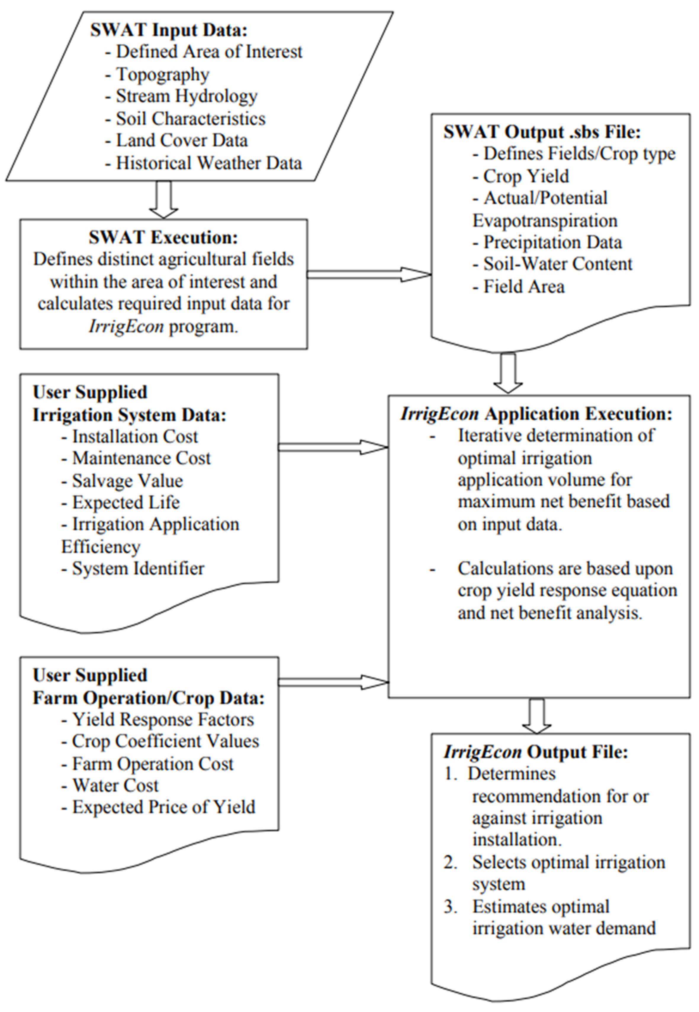
The methodology centers around the development of an independent application, programmed in Visual Basic, that is capable of utilizing SWAT output files and user-supplied information as the basis for the net benefit analysis. The program application is referred to as IrrigEcon and was developed as part of the research work being carried out at the University of Maryland. Figure 1 presents a schematic of the components of the integrated SWAT-IrrigEcon model.

2.1. SWAT Model Setup

In using the application, the first step is the development and execution of the SWAT model [16,17]. SWAT input data was obtained from freely available sources, including the National Resource Conservation Services (NRCS) Soil Data Mart [18], the National Oceanic and Atmospheric Administration (NOAA) Climatic Data Center [19], the United States Geological Survey (USGS) National Land Cover Dataset [20], the USGS National Hydrography Dataset [21], and the USGS National Elevation Dataset [22].

The SWAT model methodology, development, calibration, and execution are beyond the scope of this study. However, SWAT model input file development followed the general guidelines and procedures as outlined in model documentation [23], using the available spatial and climatic dataset sources listed above. For the purposes of this study, SWAT was used to model the Pocomoke watershed extending over 100,000 hectares, including parts of Virginia, Maryland’s eastern shore, and Delaware. The SWAT output file (* .sbs file, hru in the newer version) was then utilized in the execution of the IrrigEcon application developed for this study. In this file, the model outputs are presented for each Hydrologic Response Unit (HRU), the smallest spatial unit of the model that represents a unique combination of land uses, soils, and slopes.

2.2. IrrigEcon Development

The IrrigEcon application utilizes the SWAT output data along with economic data for expected crop production revenue values, as well as irrigation costs. The default production and revenue costs are based on the best available information for Maryland farmers as obtained from the Maryland Agricultural Statistic Service, and available marketing information obtained from irrigation dealers and service providers located within Maryland’s eastern shore. Irrigation installation costs are based on the rough estimates of a single irrigation contractor, and therefore could vary from supplier to supplier, and may change with shifting market prices. Moreover, the application is not limited to objectively comparing three distinct irrigation systems used in this study: traveling gun, center pivot, and drip irrigation. Rather, the methodology can be applied to a single system (center pivot for example), where multiple cost estimates can be obtained, each varying in the materials used, the efficiency of the design, the maintenance requirements, and the expected life of the system. The end result will be the computation of the overall net benefit associated with each system, where the system with the greatest net benefit (or the most economically optimal) is the recommended system.

It should be noted that alternative construction designs and materials used will not only affect water use efficiency and the installation cost, but may alter the expected life of the system, the salvage value, and maintenance costs of the system, all of which is taken into consideration by the model. The obvious outcome and advantage to this approach is the selection of the most economically favorable system design.

The program allows the user to overwrite, edit, and create economic datasets, in order to include more up to date or relevant economic data pertinent to the needs of the user. Once the necessary SWAT and economic/irrigation datasets have been specified, the application determines the net benefit of irrigation by a series of iterations that calculate the estimated increase in yield and associated revenue for an incremental increase in applied irrigation. The net benefit is calculated from a modified equation proposed by Mannocchi and Mecarelli [24]. The equation is shown as Equation (1) below:

$$N{B}_I=\left(Y_t\right).\left(P_s-C_1\right)-\left[\left(C_0+C_{ID}\right).A_{HRU}. 100\right]-Vo{l}_I\left(C_W\right)$$

(1)

which is simplified for the purposes of this study as the following:

$$N{B}_I =\left(Y_t\right).P_s-\left[\left(C_P+C_{ID}\right).A_{HRU}. 100\right]-Vo{l}_I\left(C_W\right)$$

(2)

• where, Y_m ≥ Y_t ≥ YLD,
• where,
• NB_I = added net benefit from irrigation ($/ha)
• Y_m = maximum yield assuming full growth (tons/ha)
• Y_t = target yield with supplemental irrigation (tons/ha)
• YLD = harvested yield without supplemental irrigation (tons/ha)
• P_s = sale price of yield ($/ton)
• C₀ = fixed cost of production per unit area ($/ha)
• C₁ = cost varying with yield ($/ton)
• C_w = cost of water per unit volume ($/m³)
• C_p = agricultural cost of production ($/ha)
• C_{I D} = irrigation installation net depreciation for the time step ($/ha)
• A_HRU = area of the HRU (km²)
• Vol_I = irrigation volume applied to HRU over the year (m³)

2.2.1. Yield Estimation

In this case, target yield (Y_t) is the yield associated with the highest net benefit. It is the sum of the expected yield without applied irrigation (YLD) and the increase in yield due to applied irrigation (ΔY). Vaux and Pruitt [25] proposed an empirical-based linear equation that relates the ratio of expected yield to maximum yield, to the ratio of actual evapotranspiration rates to potential evapotranspiration rates, through an empirically determined crop-yield response factor.

The equation was originally used to determine expected crop yield based on irrigation deficit practices in order to determine maximum irrigation deficit levels that yield acceptable results. In the case of this model, the equation has been modified in order to relate the target yield (the yield resulting in the greatest net benefit) to the associated target evapotranspiration rate:

$$1-\frac{Y}{Y_m}=k_y[1-\frac{E{T}_a}{E{T}_P}]$$

(3)

This equation is modified in the IrrigEcon application such that maximum yield and potential evapotranspiration are replaced by the target yield and the associated target evapotranspiration. Actual yield and actual evapotranspiration values are obtained from SWAT output files as determined by climatic model input variables and farm management factors entered into the SWAT model. This modified equation is shown below:

$$1-\frac{Y_a}{Y_t}=k_y[1-\frac{E{T}_a}{E{T}_t}]$$

(4)

• where,
• Y = expected crop yield (kg/ha)
• Y_m = maximum crop yield (kg/ha)
• Y_a = actual crop yield (kg/ha)
• Y_t = target crop yield (kg/ha)
• k_y = crop-yield response factor (dimensionless)
• ET_a = actual evapotranspiration (mm)
• ET_p = potential evapotranspiration (mm)

An iterative process using Equations (2) and (4) determines the target yield. In Equation (4), the target evapotranspiration is bounded by the actual transpiration without irrigation as being the minimum possible value and the potential evapotranspiration as being its upper limit, which is obtained when the maximum beneficial irrigation quantity is applied.

2.2.2. Cost Estimation

In the IrrigEcon model, agricultural production/operating costs are applied as the basic input cost for determining the net benefit value of agriculture with and/or without irrigation. The average annual operation cost is determined based on the basic cost of operating the farm and includes the cost of agricultural inputs such as seed, fertilizer, lime, pesticides, fuel, and oil, as well as service items such as repair and maintenance of capital items, machine hire, labor, marketing, storage, and transportation (details are shown in

Table A1. Itemized cost estimates for farm operations. These values represent the average seasonal price received by Maryland farmers in 2003, as reported by the Maryland Agricultural Statistics Services (MASS).

Cost Item	Cost for 2003 [Thousand Dollars]
Seed Purchased	83,039
Fertilizer and Lime	44,161
Pesticides	37,464
Petroleum Fuel and Oils	42,581
Machine Hire and Custom Work	16,106
Marketing, Storage, and Transportation	61,857
Contact Labor	12,269
Net Government Transaction	−20,302
Total	277,715

). The net operating cost is determined by summing all agricultural costs as reported by MASS (2004) and subtracting the net governmental payments, which may serve to alleviate the cost of running the farm, and divided by the total farmland acreage. The capital and maintenance cost of irrigation equipment and water is added to the above-mentioned operating costs in simulations where irrigation is applied. Given the total agricultural cropland area of 833,650 hectares (2,060,000 acres) in the state of Maryland, the average operating cost for each hectare of farmland is estimated to be USD 330/ha. The combined averaged agricultural production cost is estimated to be USD 485/ha·year based on the average farm size and the average production cost for Maryland farmers in 2003, as reported by MASS. This value is calculated by dividing the average production cost of all agricultural farms in Maryland with the average size of Maryland farms.

The variable cost associated with the operation of the irrigation system reflects the water supply cost, and:

(i) if water is obtained onsite (well water), electrical pumping cost is considered,

(ii) if water is obtained from municipal sources, market cost for water is considered.

In this study, it was assumed that water is available from the aquifer accessible from the farm site. In this study, the cost of water is estimated at a basic rate of 3 cents/m³. This estimate reflects the cost of pumping the water from shallow groundwater supplies. In this calculation, pumping efficiency is estimated to be 70%, with a pumping flow rate of 100 L/s, a total dynamic head of 40 m, and an average cost of electricity of USD 0.000823/kWh. In addition, the annual capital depreciation rate assumes the center pivot irrigation system has a 20-year life span, while both the drip system and traveling gun are expected to last about 15 years. This information, as well as the calculated annual depreciation and maintenance cost, is summarized in

Table A2. Itemized cost estimates for irrigation systems. These values represent the average seasonal price received by Maryland farmers in 2003, as reported by the Maryland Agricultural Statistics Services (MASS).

Crop Type	Acres Harvested	% of Total Crop Land	Reported Price Received by Farmer	Converted Price Received by Farmer ($/metric ton)
Corn	505,000	33.14	2.85 $/bushel	112.20
Soybean	470,000	30.84	7.25 $/bushel	266.40
Hay	220,000	14.44	150 $/ton	150.00
Wheat	180,000	11.81	3.15 $/bushel	115.75
Alfalfa	45,000	2.95	143 $/ton	143.00
Barely	4100	2.69	1.80 $/bushel	82.70
Sorghum	5000	0.33	2.55 $/bushel	100.40
Potato	4700	0.31	8.8 $/100 pounds	194.50
Vegetables	52,100	3.42	Various	Various

.

In this evaluation, the sale prices received by the farmer are assumed to be constant in spite of supply variation. Although, market prices may increase with declining supply levels (e.g., during droughts). However, for simplicity, this model considers a constant market price for all crops, under both drought and non-drought conditions. Detailed information is provided in

Table A3. The market prices used in this study. These values represent the average seasonal price received by Maryland farmers in 2003, as reported by the Maryland Agricultural Statistics Services (MASS). This table also includes the percentage of total agricultural cropland in Maryland dedicated to the production of each crop commodity in 2003.

Irrigation System	Installation Cost	Annual Depreciation	Annual Maintenance Costs	Irrigation Efficiency
Drip Irrigation	$100,000	$6700	$2000	0.95
Travelling Gun	$50,000	$3350	$2000	0.80
Center Pivot	$92,500	$4625	$1000	0.85

.

2.2.3. Irrigation Volume Estimation

The IrrigEcon application uses Equations (2) and (4) in order to determine the target yield and the associated target evapotranspiration, by incremental increases in the applied irrigation volume. The irrigation volume is related to the associated evapotranspiration level through Equations (5) and (6) below:

$$Vo{l}_I=\frac{I_D.A_{HRU}.1000}{EFI}$$

(5)

• where:
• Vol_I = irrigation volume applied to HRU over a given time step (m³)
• I_D = effective minimum irrigation depth applied (mm)
• A_HRU = area of the HRU (km²)
• EFI = total irrigation efficiency (dimensionless)

Equation (5) relates the applied irrigation volume to an effective applied irrigation depth, which depends upon the efficiency of the irrigation system. For comparison purposes, the IrrigEcon application includes default economic and system data on three irrigation systems: drip irrigation, center pivot irrigation systems, and traveling gun systems, each of which are used extensively in large-scale agricultural production systems. The IrrigEcon application assumes default efficiency values of 0.95, 0.85, and 0.80 for each of the three systems, respectively. Drip irrigation is associated with the highest efficiency value and therefore requires the least amount of water for the same effective applied irrigation depth. The traveling gun system is associated with the least efficient system, and therefore, requires the greatest amount of applied water to achieve the same effective applied irrigation depth. These default irrigation efficiency values together with the associated economic data can be modified in the IrrigEcon application in order to suit the requirements or circumstances of the user.

Once the effective irrigation depth is determined for each of the modeled irrigation systems under consideration, the target evapotranspiration is determined by Equation (6) below. Equation (6) is a simplified water balance equation used to determine the evapotranspiration rate, taking into account the applied precipitation and or precipitation during the time step, the surface runoff, percolation beyond the root zone, lateral flow, and return flow from a shallow aquifer:

$$E{T}_t=I_D+PRECIP-SQ-PERC-LQ+RVAP$$

(6)

• where:
• I_D = minimum irrigation depth applied (mm)
• ET_t = target evapotranspiration (mm)
• PRECIP = amount of precipitation falling during time step (mm)
• SQ = surface runoff during time step (mm)
• PERC = percolation past the root zone during time step (mm)
• LQ = lateral flow during time step (mm)
• RVAP = return water from shallow aquifer to the root zone (mm)

Once the target evapotranspiration rate is determined it is used in Equation (4) above in order to determine the target yield, which is substituted into Equation (2) used to calculated the net benefit of the irrigation application. This iterative process repeats itself with incremental increases in applied irrigation water, until a maximum net benefit value is achieved. The net result is the determination of a maximum net benefit associated with each of the three irrigation systems compared in the model, or each of the irrigation systems specified by the user. The irrigation system associated with the greatest net benefit value becomes the model recommended irrigation system. If the model determined net benefit is less than the net benefit of the agricultural system without irrigation, due to the associated cost of the irrigation installation and applied water, then irrigation is not recommended for the conditions specified.

In the case of this study, where the model is applied to the entire Pocomoke watershed, which is associated with a range of soil types, climatic variables, and hydrological conditions, the net benefit of irrigation will vary depending on the associated conditions. The discussion below centers on the results of the model associated with the Pocomoke region and the default input values specified.

3. Results

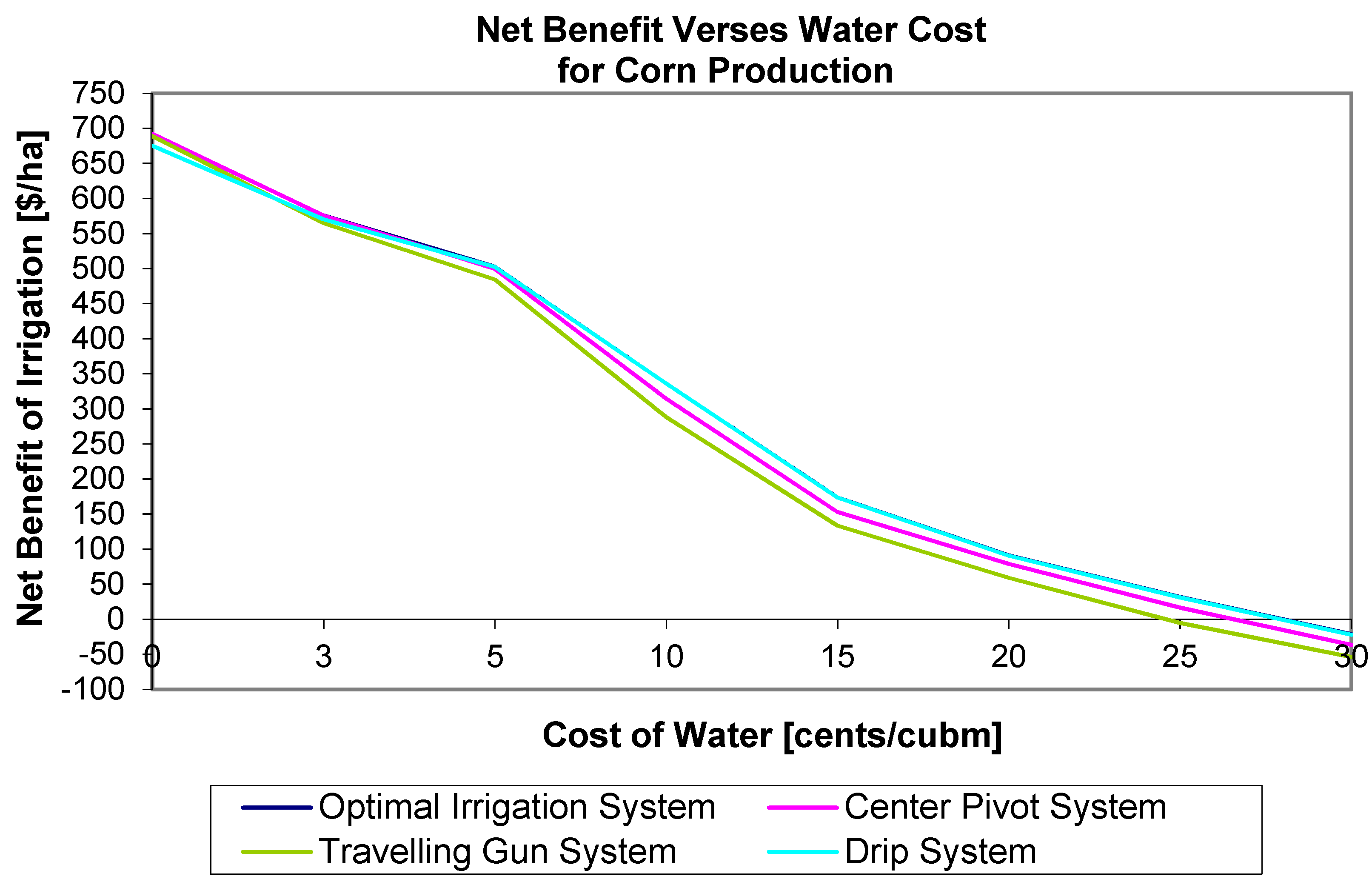
Figure 2 below compares the net benefit of each of the three systems, with the optimal or recommended irrigation system corresponding to the irrigation system with the highest net benefit for the particular conditions associated with each HRU. The overall net benefit of irrigation varied little between each of the three systems, with each system following the same trend with nearly the same magnitude (Figure 2). The net benefit presented in the graph represents the net benefit of irrigation, calculated as the difference in expected gross revenue with and without irrigation in US dollars per hectare ($/ha). Figure 2 clearly shows strongly favorable conditions for irrigation installations when water costs remain low; however, as water cost increases to 25 cents per cubic meter and beyond, irrigation no longer becomes favorable for any of the three irrigation systems included in the study. The negative net benefit values indicate that on average, higher net income can be expected for farmlands without the economic burden of irrigation equipment when compared to farmlands equipped with irrigation, given the water cost level associated with the simulation.

Table A4. Net benefit values associated with corn production for each irrigation system under various water cost values.

Cost of Water: [$/m3 of water]	Net Benefit for Optimal Irrigation System: [$/ha]	Net Benefit for Center Pivot System: [$/ha]	Net Benefit for Traveling Gun System: [$/ha]	Net Benefit for Drip Irrigation System: [$/ha]
$0.00	692.3	692.3	688.8	675.1
$0.03	575.6	575.6	564.9	570.4
$0.05	502.7	499.7	484.5	502.4
$0.10	336.2	314.6	288.1	336.1
$0.15	173.7	152.9	133.4	173.6
$0.20	91.3	78.9	59.1	90.7
$0.25	31.7	16.7	−5.1	31.2
$0.30	−21.3	−36.5	−53.8	−22.1

helps to determine the relative difference between each system. The net benefit value for each system represents the average calculated value over a 20-year simulation when all HRU’s are using the same irrigation system. The net benefit for optimal irrigation is the average calculated net benefit when the DSS selects the optimal irrigation system for each HRU, and the optimal irrigation system is selected based upon which system results in the greatest overall net benefit. Under such conditions, the center pivot system is found to be the most economically favorable for all HRU’s when the associated water cost remains below 3 cents/m³. For the water cost levels above USD 0.05/m³, the most economically favorable system is drip for each HRU. Therefore, the average net benefit for the optimal system is higher than the individual values of the three irrigation systems when viewed separately. Table A4 also indicates that the net benefit between three irrigation options was not drastically different from each other at water prices of less than USD 0.03/m³. In fact, the traveling gun option was more beneficial than the drip irrigation when water is free (i.e., USD 0.0/m³), which is the current price of water in the study region and thus resulted in adoption of traveling gun systems by some of the producers. As indicated in Table A2, the initial investment/installation cost for traveling gun is lower than both the center pivot and the drip irrigation systems. As such, there was more incentive for the farmers to select traveling gun while the water is free of charge in the study region. In addition, at the time of adoption of the traveling gun system, farmers in the region did not have access to such in-depth analysis for each of these systems in order to make a conscientious decision.

Based upon the data presented above, the center pivot system is found to be the most cost-effective system for each HRU when water costs are low (below 5 cents/m³). As the water cost increases (greater than 5 cents/m³), drip irrigation emerges as the most economically favorable system. For water cost levels at USD 0.0/m³, the most favorable system is the center pivot, and the second favorable system is the traveling gun. For water cost levels above 25 cents/m³, irrigation is no longer economically beneficial for any system.

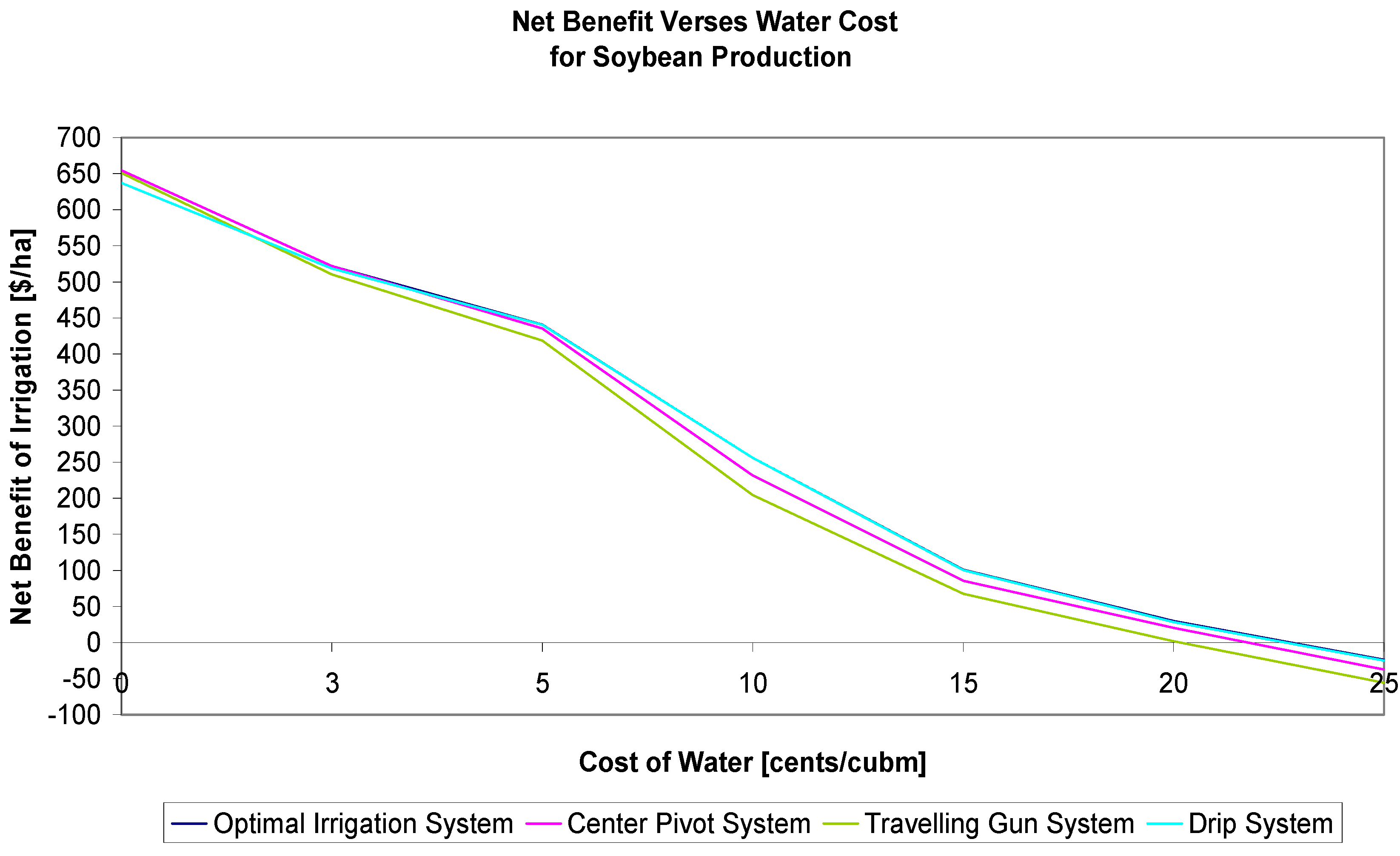
Figure 3, Figure 4 and Figure 5 below present the net benefit versus water cost for soybean, wheat, and sorghum production. In the case of soybean and wheat, the relationship between net benefit and the cost of water follows the same general trend for that of corn production for each of the three irrigation systems compared. In each case, the net benefit of irrigation decreases with the increasing water cost level until finally crop production is no longer profitable with irrigation installations.

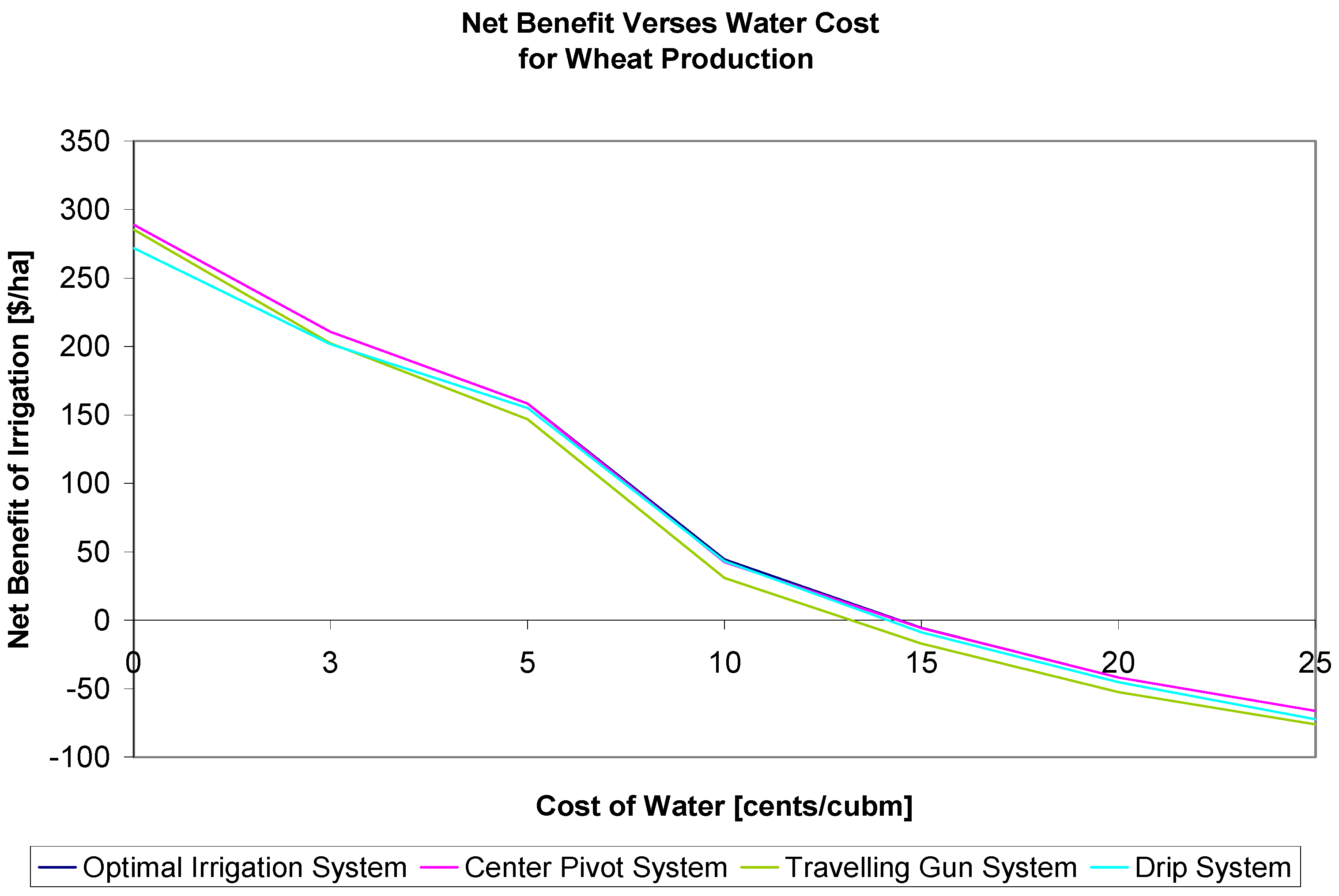
In the case of soybean production (Figure 2), irrigation remains marginally profitable up to a water cost level of 20 cents/m³, while wheat production (Figure 3) becomes unprofitable above a water cost level of 10 cents/m³. This difference is predominately due to the fact that soybean is the more valuable crop (USD 265/metric ton for soybeans compared to USD 115/metric ton for wheat), and therefore has a greater net return for crop yield increases resulting from applied water.

As in the case of corn production, center pivot irrigation emerges as the most profitable of the three systems, particularly at the lower water cost levels, while drip irrigation becomes more competitive as the cost of water increases. At a water cost level of 5 cents/m³ in the case of soybean, and 10 cents/m³ in the case of wheat, drip irrigation emerges as the most profitable of the three systems. However, the traveling gun system is the second most favorable option right after center pivot when the price of water is USD 0.0/m³ for corn, soybean, and wheat. For wheat, traveling gun remains as the second most favorable option after the center pivot for the price of water at USD 0.03/m³ or below.

As in the case of corn, drip irrigation remains the most profitable system associated with soybean production, as the water cost level increases. In the case of wheat production, the center pivot system reemerges with the highest net benefit at water cost levels of 15 cents/m³ and above. At these water cost levels, the net benefit values for wheat production, for each of the three systems, are negative. Wheat is the less valuable crop, and therefore, water application is not justified, to the same degree, at the higher water cost levels. The result is a loss of the savings normally associated with water conservation achieved through the use of drip irrigation.

In the case of sorghum production, the situation is far different. Sorghum is the least expensive of the crops compared in this analysis and the least productive in terms of yield per hectare. As a result, the annual irrigation installation and maintenance expense is too great a burden for the modest revenue generated through sorghum production. Given the economic data used in this study, sorghum production, in combination with the added cost of the irrigation system, remains unprofitable even when there is no cost associated with the water applied (Figure 5).

Table A5. Net benefit values associated with soybean production for each irrigation system under various water cost values.

Cost of Water: [$/m3 of water]	Net Benefit for Optimal Irrigation System: [$/ha]	Net Benefit for Center Pivot System: [$/ha]	Net Benefit for Traveling Gun System: [$/ha]	Net Benefit for Drip Irrigation System: [$/ha]
$0.00	654.63	654.63	651.14	637.42
$0.03	522.05	522.05	510.39	518.64
$0.05	440.72	435.44	418.82	440.58
$0.10	256.21	231.48	204.53	256.14
$0.15	100.69	85.67	67.57	100.58
$0.20	29.67	20.41	2.09	28.4
$0.25	−23.91	−37.43	−55.59	−24.88
$0.00	654.63	654.63	651.14	637.42

,

Table A6. Net benefit values associated with wheat production for each irrigation system under various water cost values.

Cost of Water: [$/m3 of water]	Net Benefit for Optimal Irrigation System: [$/ha]	Net Benefit for Center Pivot System: [$/ha]	Net Benefit for Traveling Gun System: [$/ha]	Net Benefit for Drip Irrigation System: [$/ha]
$0.00	288.94	288.94	285.46	271.73
$0.03	210.63	210.63	202.25	201.66
$0.05	158.42	158.42	146.78	154.95
$0.10	44.31	42.38	31	43.08
$0.15	−5.54	−5.71	−17.1	−8.87
$0.20	−41.79	−41.91	−52.49	−45.42
$0.25	−66.3	−66.33	−76.13	−72.43
$0.00	288.94	288.94	285.46	271.73

and

Table A7. Net benefit values associated with sorghum production for each irrigation system under various water cost values.

Cost of Water: [$/m3 of water]	Net Benefit for Optimal Irrigation System: [$/ha]	Net Benefit for Center Pivot System: [$/ha]	Net Benefit for Traveling Gun System: [$/ha]	Net Benefit for Drip Irrigation System: [$/ha]
$0.00	−0.82	−0.82	−4.3	−18.05
$0.03	−41.62	−41.62	−46.14	−57.05
$0.05	−50.4	−50.4	−54.89	−65.72
$0.10	−62.34	−62.34	−67.08	−77.39
$0.15	−71.63	−71.63	−76.75	−86.07
$0.20	−79.32	−79.32	−84.57	−93.56
$0.25	−86.38	−86.38	−92.07	−99.87
$0.00	−0.82	−0.82	−4.3	−18.05

present the tabular data associated with the figures above for soybean, wheat, and sorghum production. In the case of sorghum, as seen in Table A7, irrigation remains unprofitable for all irrigation options and that could mainly be due to the low price of sorghum.

4. Discussion

4.1. Net Benefit Statistical Analysis

The goal of this analysis was to determine those variables that differ between the HRUs, where the more expensive, more efficient drip irrigation system is associated with the highest economic advantage, and those HRUs where the less efficient but less expensive center pivot system is recommended. For each of these HRUs, the economic data applied is identical in that the same crop is grown within each agricultural HRU, receiving the same price per unit yield, and the identical economic values are applied on a per hectare basis in terms of the irrigation maintenance and installation costs and the agricultural production costs. Nevertheless, the model may or may not recommend irrigation application for individual HRUs and, in those cases where irrigation is recommended, may select different irrigation systems for distinct HRUs based on the value of specific parameters associated with each of these HRUs. These differences in irrigation system recommendations can only be attributed to the varying characteristics (soils, slope, crop type, etc.) associated with each HRU.

The analysis discussed below was conducted both laterally, considering various crops produced in Maryland and for which appropriate crop yield factor (k_y) values are available, and in-depth, by determining the factors that influence the preference of one irrigation system over another given the same production and associated economic factors. Further analysis contrasts the physical parameters of the various HRUs that influence the net benefit of irrigation for a given crop. The data included in this analysis are a composite of: the. sbs output information obtained from SWAT for each HRU, the STATSGO soil information for each soil type within the watershed and attributed to the HRU, the topography and elevation data for each sub-basin, and the irrigation system recommendation data obtained as an output of the irrigation-economic model.

4.2. Primary Factors in Determining Irrigation Application

Using the SAS ‘Mixed’ ANOVA, several factors emerged that were found to influence whether or not irrigation is recommended. The primary factors that determine irrigation recommendation are the cost of water, the water stress level of the plant, and the crop type, each of which is associated with a probability of a significant difference greater than 95%.

Table 1. Results of analysis of variance (ANOVA) in determining the factors that influence model recommendations for the application or non-application of irrigation.

Model Parameters	Parameter Description	F-Value	Associated Probability
WATERCOST	Cost of water per unit volume	3248.87	<0.0001
LULC	Crop produced	6.77	0.0093
AREA	Area of the HRU	0.76	0.3842
SYLD	Sediment yield	3.41	0.0650
SEDP	Sediment bound phosphorus	0.04	0.8492
WSTRS	Degree of water stress	9.87	0.0017
NSTRS	Degree of nitrogen stress	0.08	0.7711

Note: In all cases, the numerator degrees of freedom is 1, and the denominator degrees of freedom is 6406.

below lists the various parameters considered in the ANOVA and the determined f-value and associated probability.

Of the factors listed above, the most significant factor in determining if irrigation is or is not recommended is the cost of water, with an associated probability of less than 0.0001. This is clearly apparent when considering the graphs of recommended irrigation volumes presented in the previous section. Low water cost leads to significant and widespread water application recommendations for all crop types, while high water costs lead to reduced water application recommendations.

The next most significant factor in determining irrigation application is the degree of water stress associated with each crop type. The factors that influence water stress for an identical weather pattern are soil conditions, plant physiology, and the crop’s tolerance to drought conditions as represented by its k_y value.

The third most significant factor in determining irrigation application is the type of crop being produced. In this study, soybean production is associated with the highest water volume application, varying from 4434 to 1062 m³/year for the various water cost levels modeled, while sorghum is associated with the least amount of recommended irrigation, varying from 2168 to 141 m³/year depending on the water cost level.

4.3. Primary Factors in Irrigation System Recommendations

The discussion that follows also used ANOVA, but considered the model recommended irrigation system as the dependent variable. In this case, the cost of water and the water stress intensity emerged as the most significant factors in determining the recommended irrigation system (

Table 2. Results of analysis of variance (ANOVA) in determining the factors that influence the model irrigation system recommendation.

Model Parameters	Parameter Description	F-Value	Associated Probability
WATERCOST	Cost of water per unit volume	1078.17	<0.0001
LULC	Crop produced	2.75	0.0970
AREA	Area of the HRU	0.85	0.3553
SYLD	Sediment yield	1.65	0.1987
SEDP	Sediment bound phosphorus	0.00	0.9521
WSTRS	Degree of water stress	21.46	<0.0001
NSTRS	Degree of nitrogen stress	1.93	0.1647

Note: In all cases, the numerator degrees of freedom is 1, and the denominator degrees of freedom is 6406.

). The three irrigation systems considered are associated with various efficiency values, and therefore require different volumes of water for the same net effect. As a result, the cost of water is one of the primary factors in irrigation system selection. Next in line is the water stress intensity of the crop, which is correlated with the water demand. The water stress intensity becomes a more relevant factor in determining the recommended irrigation system as water costs rise. At lower water cost levels, the water demand is more easily met by all irrigation systems with less effect on the overall net benefit. Table 2 lists the various parameters considered in the ANOVA and the determined f-values and associated probability to determine the factors that influence the model irrigation system.

4.4. Primary Factors Influencing the Annual Net Benefit of the System

Using the maximum net benefit as the dependent variable in the ANOVA test results in the determination of a wider range of variables that are significant in determining the annual net benefit of irrigation. These variables include: the cost of water, the crop produced, USLE, water stress intensity, and degree of nitrogen stress. Of these variables, the primary factors include the economic variables that determine production costs and revenue, such as the cost of water and value of the crop (

Table 3. Results of analysis of variance (ANOVA) in determining the factors that influence annual net benefit values.

Model Parameters	Parameter Description	F-Value	Associated Probability
WATERCOST	Cost of water per unit volume	17,142.4	<0.0001
LULC	Crop produced	20.37	<0.0001
AREA	Area of the HRU	0.36	0.5508
SYLD	Sediment yield	0.55	0.4593
SEDP	Sediment bound phosphorus	0.06	0.7998
WSTRS	Degree of water stress	11.7	0.0006
NSTRS	Degree of nitrogen stress	9.57	0.0020

Note: In all cases, the numerator degrees of freedom is 1, and the denominator degrees of freedom is 6406.

). These variables also include the water stress and nitrogen stress experiences as these factors affect plant growth and subsequently the productivity of the system.

5. Conclusions

The objective of this study was to develop a decision support tool for farmers in temperate regions to evaluate the cost-benefit of irrigation installations. Optimal irrigation system selection is found to depend most heavily upon the price of water and the installation and maintenance costs of the system. Results of this study indicated that during successive simulations, as the cost of water increased, drip irrigation characterized by higher installation and maintenance costs, but higher water use efficiency, was increasingly recommended as the most economically beneficial system. This was true due to its added savings achieved through water conservation. Under the simulation and economic conditions defined in this project, the traveling gun irrigation system, characterized by low installation costs, higher maintenance, and low irrigation distribution efficiency, was found to be the least economical of all systems. However, an overall trend was observed in which traveling gun systems became more economically favorable than drip irrigation as the cost of water decreased and/or water was free of charge (USD 0.0/m³), although the associated net benefit remained beneath that of center pivot systems at all times.

Initially, it was believed that irrigation system selection may depend, to a more significant degree, on the physical characteristics of the terrain and the associated properties of the HRU. It was believed that this sort of modeling could more clearly delineate between HRUs that favor more water-efficient systems and those HRUs that profit more from less expensive but less conservative systems. Such diversification of irrigation system recommendations did occur to a limited degree, however it was overshadowed by the influence of the cost of water and irrigation installation costs. Nevertheless, to a discernable degree, model recommendation variation did occur, recommending the most economically favorable system based upon the physical characteristics of widely different HRUs, given the same set of initial economic conditions.

References

- Wheeler, J.C. Freshwater Use Trends in Maryland, 1985–2000; US Department of the Interior, US Geological Survey: Reston, VA, USA, 2003.
- Paul, M.; Dangol, S.; Kholodovsky, V.; Sapkota, A.R.; Negahban-Azar, M.; Lansing, S. Modeling the Impacts of Climate Change on Crop Yield and Irrigation in the Monocacy River Watershed, USA. Climate 2020, 8, 139. [Google Scholar] [CrossRef]
- MDA. Agriculture in Maryland: Summary for 2010; Maryland Department of Agriculture: Annapolis, MD, USA, 2010.
- Hanna, K. Integrated Economic Decision Support System Model for Determining Irrigation Application and Projected Agricultural Water Demand on a Watershed Scale (Doctoral Dissertation); University of Maryland: College Park, MD, USA, 2006. [Google Scholar]
- Doorenbos, J.; Kassam, A. Yield Response to Water; Food and Agriculture of the United Nations: Rome, Italy, 1979. [Google Scholar]
- Gardner, W.R. Availability and measurement of soil water. In Water Deficits and Plant Growth; Kozlowski, T.T., Ed.; Academic Press: New York, NY, USA, 1968; Volume 5, pp. 107–136. [Google Scholar]
- Hargreaves, G.H.; Samani, Z.A. Economic consideration of deficit irrigation. J. Irrig. Drain. 1984, 110, 343–458. [Google Scholar] [CrossRef]
- Klocke, N.L.; Currie, R.S.; Tomsicek, D.J.; Koehn, J.W. Sorghum response to deficit irrigation. Trans. ASABE 2012, 55, 947–955. [Google Scholar] [CrossRef]
- Kirda, C. Deficit irrigation scheduling based on plant growth stages showing water stress tolerance. Deficit Irrig. Practices FAO Water Rep. 2002, 22, 3–10. [Google Scholar]
- Kirda, C.; Kanber, R. Water, no longer a plentiful resource, should be used sparingly in irrigated agriculture. In Crop Yield Response to Deficit Irrigation; Kirda, C., Moutonnet, P., Hera, C., Nielsen, D.R., Eds.; Kluwer Academic Publishers: Dordrecht, The Netherlands, 1999; Volume 1, pp. 1–20. [Google Scholar]
- Pereira, L.S.; Teodoro, P.R.; Rodrigues, P.N.; Teixeira, J. Irrigation scheduling simulation: The model ISAREG. In Tools for Drought Mitigation in Mediterranean Regions; Springer: Dordrecht, The Netherlands, 2003; pp. 161–180. [Google Scholar]
- Smith, M. CROPWAT: A computer program for irrigation planning and management (No. 46). Food Agric. Org. 1992, 1, 3–10. [Google Scholar] [CrossRef]
- Smith, M.; Kivumbi, D. Use of FAO CROPWAT model in deficit irrigation studies. FAO Water Rep. 2002, 22, 17–28. [Google Scholar]
- Plauborg, F.; Andersen, M.N.; Heidmann, T.; Olesen, J.E. MARKVAND: A decision support system for irrigation scheduling. In Evapotranspiration and Irrigation Scheduling, Proceedings of the International Conference, San Antonio, TX, USA, 3–6 November 1996; American Society of Agricultural Engineers: Saint Joseph, MI, USA; pp. 527–535.
- Linda, L.; Watt, J.; Vincent, K. A prototype DSS to evaluate irrigation management plans. Comput. Electron. Agric. 1998, 21, 195–205. [Google Scholar]
- Arnold, J.G.; Williams, J.R.; Srinivansan, R.; King, K.W. SWAT-Soil and Water Assessment Tool; USDA-ARS: Temple, TX, USA, 1996. [Google Scholar]
- Arnold, J.G.; Srinivasan, R.; Muttiah, R.S.; Williams, J.R. Large Area Hydrologic Modeling and Assessment Part I: Model Development. J. Am. Water Resour. Assoc. 1998, 34, 73–90. [Google Scholar] [CrossRef]
- NRCS (Natural Resources Conservation Service). Soils Data Mart. 2006. Available online: http://soildatamart.nrcs.usda.gov (accessed on 24 July 2006).
- NOAA (National Oceanic & Atmospheric Administration). NOAA Satellites and Information National Climatic Data Center. 2006. Available online: http://www.ncdc.noaa.gov/oa/ncdc.html (accessed on 24 July 2006).
- USGS (United States Geological Survey). National Land Cover Dataset. 2006. Available online: http://landcover.usgs.gov/natllandcover.asp (accessed on 24 July 2006).
- USGS. National Hydrography Dataset. 2006. Available online: http://nhd.usgs.gov/ (accessed on 24 July 2006).
- USGS. National Elevation Dataset. 2004. Available online: http://ned.usgs.gov/ (accessed on 24 July 2006).
- Neitsch, S.L.; Arnold, J.G.; Kiniry, J.R.; Srinivasan, R.; Williams, J.R. Soil and Water Assessment Tool User’s Manual-Version 2000. In TWRI Report TR-192; Texas Water Resources Institute: College Station, TX, USA, 2002. [Google Scholar]
- Mannocchi, F.; Mecarelli, P. Optimization analysis of deficit irrigation systems. J. Irrig. Drain. Eng. 1994, 12, 484–502. [Google Scholar] [CrossRef]
- Vaux, H.J.; Pruitt, W.O. Crop-water production functions. In Advances in Irrigation; Hillel, D., Ed.; Academic Press: New York, NY, USA, 1983; Volume 2, pp. 61–93. [Google Scholar]
Figure 1.
General overview of the SWAT-IrrigEcon model showing the required model inputs and selected outputs.
Figure 2.
Irrigation system comparison of net benefit versus water cost associated with corn production.
Figure 3.
Irrigation system comparison of net benefit versus water cost associated with soybean production.
Figure 4.
Irrigation system comparison of net benefit versus water cost associated with wheat production.
Figure 5.