Phytoplankton Time-Series in a LTER Site of the Adriatic Sea: Methodological Approach to Decipher Community Structure and Indicative Taxa

Abstract

In the shallow and landlocked northeast Adriatic Sea, environmental factors have changed in recent decades. Their influence on seasonal and inter-annual variability of phytoplankton has been documented in the recent literature. Here, we decipher the long-term variability of phytoplankton phenology at a Long-Term Ecological Research site (Gulf of Trieste, Slovenia). Structural changes in the phytoplankton community (period 2005–2017) were analysed using a multivariate protocol based on Bayesian clustering. The protocol was modified from the literature to fit the needs of the study, using correspondence analysis and k-means clustering. A novel index for ordination and selection of taxa based on frequency and evenness was developed. The Total Inertia analysis showed that this index better preserved the available information. Typical seasonal assemblages were highlighted by applying the Indicative Value index in conjunction with likelihood ratio values. We obtained a rough picture of the seasonal separation of the diatom-dominated community from the mixed community and a refined picture of the phenology of the assemblages and bloom events. The spring diatom peak proved to be inconstant and short-lived, while the autumn bloom was generally long and diverse. As expected for nearshore environments, the average life span of the assemblages was found to be short-periodic (2–4 months). The second part of the year and the last part of the series were more prone to changes in terms of typical assemblages.

1. Introduction

The theory behind the spatio-temporal distribution of phytoplankton species in the pelagic habitat [1] has long been debated and remains unresolved. Variations in coastal ecosystem properties play an important role in the distribution of phytoplankton taxa [2] and one of the most evident features of seasonal phytoplankton dynamics is cyclic behaviour [3,4,5,6]. Nevertheless, the core problem remains that phytoplankton taxa take on some paradoxical aspects when we consider their distribution in their hyperspace-niche [1]. The excess in phytoplankton taxa richness—the so-called Paradox of Plankton—has been associated with the permanent failure to reach the equilibrium state within the pelagic habitat, as the habitat properties vary at a similar rate as the phytoplankton reproduce [7]. Numerical simulations [8] have shown that nested competition for multiple limiting resources can lead to an unstable equilibrium, as described for phytoplankton by Hutchinson [1]. However, it is still unknown how much of the observed coexistence can be attributed to environmental heterogeneity and how much arises within the community [9].

In the 1970s, Margalef [10] introduced the concept of phytoplankton succession, the so-called Mandala, in which the main stages of succession are driven by turbulence and nutrient availability. Succession starts in highly turbulent waters where diatoms successfully proliferate (r strategy) and culminates in calm oligotrophic waters where dinoflagellates dominate (K strategy). Coccolithophores thrive in intermediate conditions, while red tides occur in calm but nutrient-enriched waters. Successive attempts have been made to revise the original mandala, but with doubtful success [11].

For our understanding of oceanic biogeochemical cycles, trophic interactions and, in general, the ecology of the marine environment, it is important to know how phytoplankton diversity is distributed in the pelagic habitat [12,13]. In the marine environment, it is particularly difficult to define areas or, better, defined spatial and temporal units on which diversity is then calculated and assemblages defined. These difficulties arise from the dynamic nature of the sea [14]. Phytoplankton phenology patterns vary in the time domain from stable annual fluctuations in certain biomes to the absence of a repeating pattern in others [15]. The usual pattern for estuarine and coastal environments is a short period with fluctuations on the order of 2–4 months [16]. Although it is often difficult to access data with spatial and temporal coverage, data from LTER (Long-Term Ecological Research) sites are ideal for studying phytoplankton phenology because they cover large time windows. Such data allow us to capture the basic community structure and its variability [16].

In the northernmost part of the Adriatic Sea, the Gulf of Trieste (GoT), phytoplankton community composition has been described as nanoflagellate-dominated, with seasonal outbursts of diatoms in spring and autumn in correlation with freshet periods and water column mixing [5,17]. This community is also sensitive to freshwater inputs [3], and some characteristic shifts in taxa composition have been observed following freshwater pulses [18,19].

One approach to analysing phytoplankton phenology is to use time series of species composition coupled with fidelity-specificity indices to describe indicative species phenology. Such an analysis has already been applied in studies in the northern Adriatic [5,20,21,22], based on fixed time intervals (seasons, months, years) used to find indicative species and describe the phenology of co-occurring species (assemblages). In this work, we propose a different approach with the reverse order of steps: species composition within time series is first used to define time intervals, and then it is possible to find the groups of indicative species within time intervals. For this purpose, we applied and modified the protocol proposed by Souissi et al. [23] and used by Anneville et al. [24] in a study on the phytoplankton community of Lake Geneva and tested for marine phytoplankton communities in the GoT [25,26].

In addition to co-occurrences, we were also interested in describing the major abundance peaks and the taxa responsible for these peaks. To estimate the distributional structure of a group of taxa, diversity indices of various kinds can usually be used to estimate, for each sample, how much abundance is concentrated or even across taxa [27]. Again, we used the same approach, but in reverse, to estimate how much the abundance is concentrated or uniform across samples for each taxon. The taxa that would be uniform would be those that have constant abundance across samples; the more they would be uneven the more their abundance would be concentrated in a few samples. In this way, we tried to be careful not to discard any important taxa during the selection process.

Upon re-analysis of the long-term phytoplankton data series from the Slovenian LTER station, we found that several problematic passages resulted in the loss of relevant information about community structure, introduced incorrect ordinations of the data, and caused difficulties in assigning indicative taxa. Therefore, one of the two goals of this study is to refine the critical passages in the protocol of the analysis. The other objective of this study is to use the refined analysis steps to better characterize the temporal dynamics of phytoplankton with the determination of characteristic periods and species at the Slovenian marine LTER station in the GoT.

2. Materials and Methods

2.1. Area of Study

The Gulf of Trieste (GoT) is a basin surrounded by land at the northeastern tip of Adriatic Sea. Due to its shallow depth, 21 m on average [28], the GoT is largely influenced by climatic conditions that cause variations in salinity and temperature. The GoT is seasonally stratified, and its euphotic zone significantly exceeds the depth of the upper mixed layer for most of the year [29]. The basin is under the influence of two main winds, the “bora” and the “jugo”, which blow from the northeast and southeast, respectively. Bora is a strong catabatic wind whose effect on the water column is twofold: mixing and cooling, while Jugo is a constant wind that is thought to have a chaotic effect on the current circulation in the Gulf [30].

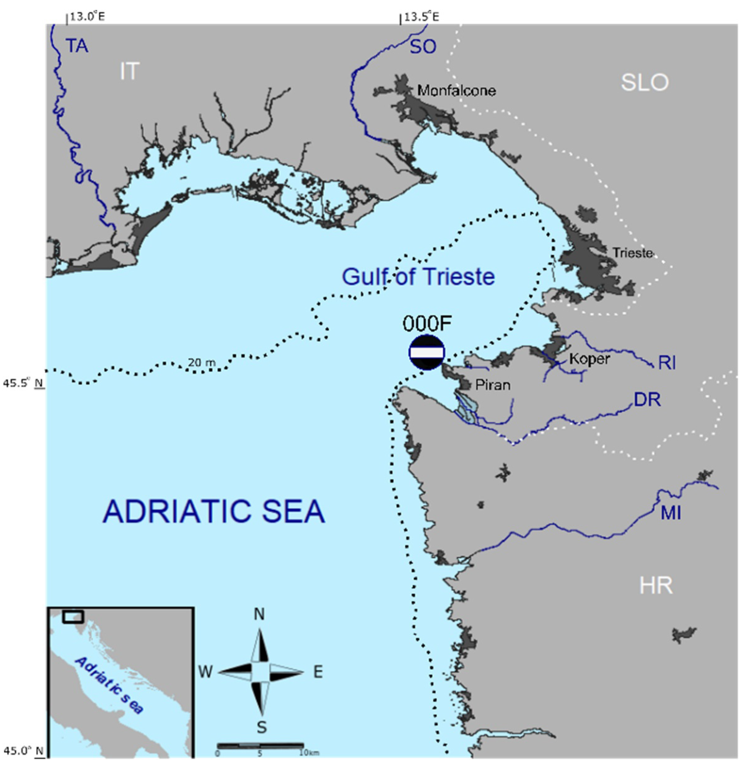
The Slovenian LTER station (45.53833° N, 13.55° E; 21 m depth) is located at the southern entrance to the GoT (Figure 1), where direct impact from freshwater inputs and other pressures are minimal. The waters around the station are usually traversed by the current North Adriatic Dense Water (NAdDW). Only occasionally, they are reached by the plume of the Soča (Isonzo) River (SO, Figure 1), one of the local freshwater sources that has the greatest influence on the basin [30]. The Slovenian LTER station represents the reference station for national monitoring purposes, but the bias of the representation should be taken into account when generalizing the results to the whole Gulf.

2.2. Data

Monthly data from Slovenian LTER sampling station 000F (Figure 1) were collected and stored as part of routine sampling in the Slovenian National Monitoring Program. In this work, a twelve-year time series from 2005 to 2017 was analysed. Phytoplankton was sampled with Niskin bottles (5 L) at different depths (0 m, 5 m, 15 m and near the bottom at 21 m). Phytoplankton samples were fixed with neutralized formaldehyde and stored until analysis. Subsamples of 50 mL were left to settle in a sedimentation chamber for 48 h and then examined using an inverted microscope ZEISS Axiovert 135, according to the Utermöhl method [31]. Phytoplankton taxa were determined to the lowest possible taxonomic level and counted in 50 to 100 microscope fields at 400× magnification. The final dataset of phytoplankton composition and abundance included more than 100,000 entries. Taxonomic names were verified according to recent changes and consistency was checked for synonyms [32,33].

2.3. Analysis

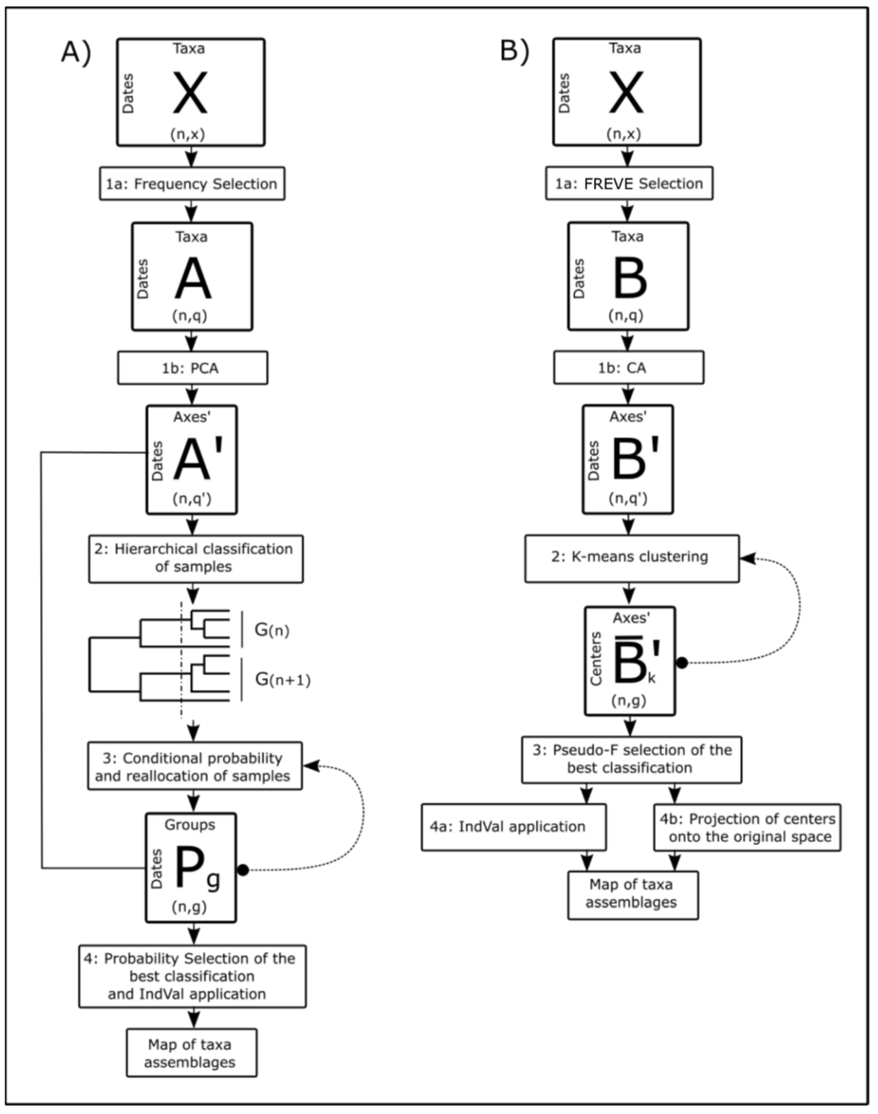
Data analysis was performed using R-studio software (Version 1.1.456—© 2021–2018 RStudio, Inc., Boston, MA, USA).

Table A1. List of R-packages and functions used in the analysis.

Package	Functions	Goal
vegan [56]	diversity	Pielou λ
ade4 [57]	dagnelie.test	Multinormality
	dudi.coa	CA
cluster [58]	agnes	Hierarchical classification
Morpho [59]	typprobClass	Probability from Mahalanobis
cclust [38]	clustIndex	Calinski & Ratkowsky
labdsv [60]	indval	IndVal indexes
ape [61]	mantel.randtest	Mantel test

in Appendix A shows the list of packages used in the analysis. Prior to analysis, data from different depths were merged in the Integrated Abundance (IA) using the trapezoidal rule. On the resulting matrix of taxa IAs (matrix X; Figure 2), a series of statistical methods for clustering the samples proposed by Anneville et al. [24] were applied (Figure 2A) and then modified (Figure 2B). The core idea was to create a clustering system of the samples based on the distribution of taxa and then obtain the indicative taxa for each cluster by the index of Fidelity and Specificity (IndVal) [34].

2.4. Original Protocol

The first step consisted of the selection of the taxa on which to perform the successive analysis. Following Anneville et al. [24], taxa present in less than 12% of the samples were excluded (matrix A; Figure 2A, step 1a). A Principal Component Analysis (PCA) was then applied to the log-transformed data (Figure 2A, step 1b). Principal components that accounted for 90% of the variance were retained and used to calculate PCA scores (matrix A’; Figure 2A). Multinormality was tested using the Dagnelie method [23]. From the matrix of PCA scores, hierarchical classification of samples (dates) was performed using Euclidean distance with a flexible clustering strategy (Figure 2A, step 2). Then, the probability that each sample belongs to each of the obtained clusters was calculated using Bayes’ theorem. Here, the frequency of the cluster was used as the prior probability and the conditional probability was calculated using the χ² distribution estimator of the Mahalanobis distance of the object from the centroid of the cluster [24]. Since the probability was obtained for each samples’ possible cluster, each sample could be reallocated to the cluster in which it had the maximum probability. Finally, new clusters were obtained and step 3 (calculation of P and reallocation of samples, Figure 2A) was repeated until the composition of the clusters remained stable and the final partition of the samples was obtained (matrix Pg, Figure 2A). Since it is possible to divide the samples into n clusters, where n varies from 1 to the total number of samples, a probability-based criterion was applied to characterize each partition (Figure 2A, step 4) as follows: a vector P_max(k) representing the maximum probability for each sample was calculated. Each partition was evaluated on the basis of the median of the values of P_max(k) This median was interpreted as the average measure of the within-cluster homogeneity [23]. The final clusters were used to create the map of taxa assemblages, in which each sample (i.e., each month) was assigned to a cluster (Figure 2A, step 4).

In each of these clusters, the IndVal index [34] was calculated for each taxon using the IA matrix obtained at the beginning (matrix A; Figure 2A). This index is a multiplication of two independently calculated values: the fidelity (FI_j,t) and the specificity (SP_j,t) of taxon t in the cluster of samples G_j (Equations (1) and (2), respectively).

$${\mathrm{FI}}_{\mathrm{j},\mathrm{t}}=\frac{{\mathrm{NS}}_{\mathrm{j},\mathrm{t}}}{{\mathrm{NS}}_{\mathrm{j}+}}$$

(1)

$${\mathrm{SP}}_{\mathrm{j},\mathrm{t}}=\frac{{\mathrm{NI}}_{\mathrm{j},\mathrm{t}}}{{\mathrm{NI}}_{+\mathrm{j}}}$$

(2)

where NS_j,t is the number of samples in cluster G_j containing taxon t, NS_j+ is the total number of samples in G_j, NI_j,t is the mean abundance of taxon t in the samples belonging to G_j and NI_+j is the sum of the mean abundances of taxon t in all clusters. The fidelity of a taxon for a cluster is 1 if that taxon is present in all samples of the cluster, while the specificity of a taxon for a cluster is 1 if that taxon is present only in the cluster under consideration. The IndVal is calculated as in Equation (3) and has a range between 0 and 1.

$${\mathrm{IndVal}}_{\mathrm{j},\mathrm{t}}={\mathrm{FI}}_{\mathrm{j},\mathrm{t}}\times {\mathrm{SP}}_{\mathrm{j},\mathrm{t}}$$

(3)

As established by the authors in [34], an IndVal value greater than 0.25 is considered a threshold to describe a taxon as indicative of a particular cluster.

2.5. Modified Protocol

2.5.1. Frequency Selection

In step 1a (Figure 2A), taxa were selected for analysis based on their frequency with the threshold of 12%. The distribution of log cumulative abundances of the taxa along the frequency values is shown in Figure 3A. The dashed line representing the 12% presence shows no clear discontinuity in the data to support the setting of the threshold. Furthermore, any value of frequency used as a threshold would be arbitrary as there are no discontinuities along the frequency values. This is also supported by the frequency histogram showing the relative abundances (Figure 3B), where some of the rarely occurring taxa (<12%) showed relatively high abundances (darker colour). In contrast, some of the taxa with high frequency showed relatively low abundance (lighter colour).

The lower bound of the distribution of points in Figure 3A resembles the logarithmic function. A similar shape is obtained by the log transformation of the vector of positive naturals N⁺ [1, 2, 3, …]. This distribution results from the taxa identification and counting method, during which some of the taxa were found only once per sample. This value of 1cell was then transformed per volume of sample and integrated. The resulting abundances were thus generated by a categorical process of presence/absence discrimination, even though the values look quantitative. The taxa abundances that occupy the lower limit of the distribution (those that are close to the ln(x) function, Figure 3A) are therefore the result of a scaled version of the log transformation of the presences’ vector of rare taxa. This particular distribution of some taxa led to the postulation of the co-presence of two types of rarity and four types of distribution of taxa in our dataset. A taxon may be rare in terms of frequency (i.e., observed in a small number of samples) or rare in terms of abundance (i.e., having low abundances). The combination of rarities results in four distribution types: taxa that are rare in both presence and abundance (type 1), taxa that are rare in presence but not in abundance (type 2), taxa that are common in presence and abundance (type 3), and taxa that are common in presence and rare in abundance (type 4).

To measure the evenness of the abundances of each taxon, in order to exclude the type 1 (rare and even) taxa, we chose the Pielou Evenness index λ [27]. The idea was to scale the taxa frequency (f) to the taxa evenness (λ). In this way, we obtained a new index for the taxa, which we tentatively called FREVE (frequency and evenness), and which is shown in Equation (4):

$$\mathrm{FREVE}={\mathrm{f}}^{\mathsf{\lambda }}$$

(4)

and have the limits as in Equations (5)–(8):

$$\underset{\left(\mathrm{f},\mathsf{\lambda }\right)\to \left(0^{+},1^{-}\right)}{\lim }{\mathrm{f}}^{\mathsf{\lambda }}=0$$

(5)

$$\underset{\left(\mathrm{f},\mathsf{\lambda }\right)\to \left(0^{+},0^{+}\right)}{\lim }{\mathrm{f}}^{\mathsf{\lambda }}=1$$

(6)

$$\underset{\left(\mathrm{f},\mathsf{\lambda }\right)\to \left(1^{-},0^{+}\right)}{\lim }{\mathrm{f}}^{\mathsf{\lambda }}=1$$

(7)

$$\underset{\left(\mathrm{f},\mathsf{\lambda }\right)\to \left(1^{-},1^{-}\right)}{\lim }{\mathrm{f}}^{\mathsf{\lambda }}=1$$

(8)

Infrequent taxa with evenly distributed abundance would have frequency (f) close to 0 and evenness (λ) close to 1, then FREVE is close to 0 (Equation (5)). The other three cases, corresponding to distributions of type 2 (Equation (6)), type 3 (Equation (7)), and type 4 (Equation (8)), would yield FREVE values close to 1 (Figure 3C). The histogram of the FREVE index (Figure 3D) shows how the index shifted the taxa with the highest abundances to the right half. The cutting threshold we set to select taxa was the composite of two arbitrary thresholds. Because we wanted to retain taxa that were present at least once per year (f = 1/12) and whose abundance was less uniform than the level of intermediate evenness (λ = 0.5) [35], we obtained the threshold using the Equation (4) (0.28). Finally, taxa with FREVE > 0.28 were retained for subsequent analysis.

2.5.2. Component Space and Clustering

The choice of Principal Component Analysis (PCA) in the original protocol implies the preservation of Euclidean Distance between sample objects. The use of symmetric coefficients (as Euclidean distance) for the analysis of sample-taxa datasets is not the right choice in most cases [36]. This is due to the different information that a double presence or double absence of a given taxa brings, namely the “double-zero” problem [36]. Instead of PCA, a Correspondence Analysis (CA), which preserves χ² distance, was performed on the dataset after FREVE taxa selection (Figure 2B, step 1b). CA was also used to perform Inertia analysis [36] on the datasets selected by both protocols (Figure 2A, matrix A’ and 2B, matrix B’) to evaluate and confront the two selection methods (frequency-based vs. FREVE). To obtain clusters of samples, non-hierarchical k-means clustering [36] was then computed instead of Bayesian reallocation (Figure 2B, step 2). Each n-partition was evaluated using Calinski pseudo-F [36,37] and Ratkowsky index [38] (Figure 2B, step 3).

2.5.3. Indicative Taxa

The selection of the best clustering of samples was followed, as in the original protocol, by the application of the IndVal index (Figure 2B, step 4a). Dufrene and Legendre stated that “the use of IndVal removes any effect of the number of sites in the various clusters and also differences in abundance among sites belonging to the cluster” [34]. However, with the way IndVal is calculated, it is possible for a taxon to have the same IndVal value in two completely different hypothetical situations. In the first situation, the taxon whose cumulative abundance is split into two clusters and is present in half of the samples in both clusters would have the same IndVal value in both clusters (0.25). The IndVal value would also be the same (0.25) in a second situation where the taxon is present in two clusters, where in one it is present in every sample (FI = 1) and has 25% of the abundance (SP = 0.25) and in the other it is present in one third of the samples (FI = 0.33) and has 75% of the abundance (SP = 0.75). Theoretically, it should be possible to disentangle these biased cases using the p-values calculated according to the permutative method proposed by Dufrene and Legendre [34]. However, in the multivariate situation where each cluster is defined around several taxa, many if not all taxa are suboptimally described. As a result, many of the possible cluster permutations will produce higher IndVal values for each taxon, reducing the discriminatory power of the p-value. To facilitate interpretation of the IndVal results, the centroids of the clusters (CA centroids) obtained from k-means were projected onto the space of taxa (CA columns) (Figure 2B, step 4b), resulting in a vector of taxa likelihood ratios (Observed/Expected) for the centroids. This is justified in Appendix B. The higher the projected value of the taxa (Xproj), which represents the likelihood of the centroid, the stronger the association (Xproj > 0; Likelihood ratio > 1) between the column (taxa) and the centroid (cluster). Xproj was used as the association index and the threshold was set to Xproj 1 (Likelihood ratio 2). A taxon with Xproj > 1 is strongly associated with the cluster, indicating that its observed abundance is more than twice as high as expected. The similarity of the two indicator matrices (IndVal and Xproj) was tested using the Mantel test over ranked indices (999 permutations) [36].

2.5.4. Log-Transformation

A final remark concerns the log transformation made at the beginning of the original protocol. In the modified protocol (Figure 2B), the raw data were not log-transformed because, as pointed out in the literature [39], this method, used on count data, is either redundant or wrong in most cases. In the context of extrapolating probabilities from Mahalanobis distances, multinormality was an issue and indeed, taxa abundances were log-transformed (see Section 2.4) and multinormality was tested using the Dagnelie method [23] before proceeding. However, no normality assumptions are required when using raw distances for clustering.

3. Results

3.1. Phytoplankton Community Composition and Taxa Selection

In the phytoplankton community at the Slovenian LTER station, a total of 130 taxa were determined during 2005–2017, including 53 diatom taxa, 50 dinoflagellate taxa and 15 coccolithophore taxa. The remaining 12 taxa were distributed among the classes Cryptophyceae, Chlorophyceae, Euglenophyceae, Prasinophyceae, Chrysophyceae, Dictyochophyceae and other undetermined nanoflagellates. Nanoflagellates accounted for the largest proportion of abundance (57%), while diatom cells accounted for 36%, coccolithophores 4% and dinoflagellates 3% of total abundance.

Abundance peaks above 1 × 10⁶ cells L⁻¹ were mainly recorded in late winter/spring and autumn and were mainly attributable to diatoms. Five diatom blooms were dominated by Chaetoceros spp. in February 2007 (2.2 × 10⁶ cells L⁻¹), November 2011 (1.2 × 10⁶ cells L⁻¹), November and December 2012 (up to 1.6 × 10⁶ cells L⁻¹) and July 2015 (1.7 × 10⁶ cells L⁻¹), while Skeletonema species were responsible for two February blooms in 2011 and 2012 (1.2 × 10⁶ cells L⁻¹). The largest diatom bloom was recorded in November 2010, when species from the Pseudo-nitzschia delicatissima group reached 3.7 × 10⁶ cells L⁻¹. Nanoflagellates caused two abundance peaks in July 2005 (1.5 × 10⁶ cells L⁻¹) and in May 2016 (1.6 × 10⁶ cells L⁻¹).

Out of a total of 130 taxa, 57 taxa were selected for further analysis based on the proposed FREVE (

Table 1. Comparison of the number of retained and discarded taxa between two selection methods: frequency-based and FREVE.

			Frequency Selection
			Common (f > 0.12)	Rare (f < 0.12)
			73	57
FREVE selection	(FREVE > 0.28)	57	56	1
	(FREVE < 0.28)	73	17	56

). Of these, 56 were already included in the frequency-based selection and one rare taxon was rescued. The major difference between the two selection methods was 17 common taxa that were discarded by FREVE but would have been retained based on frequency.

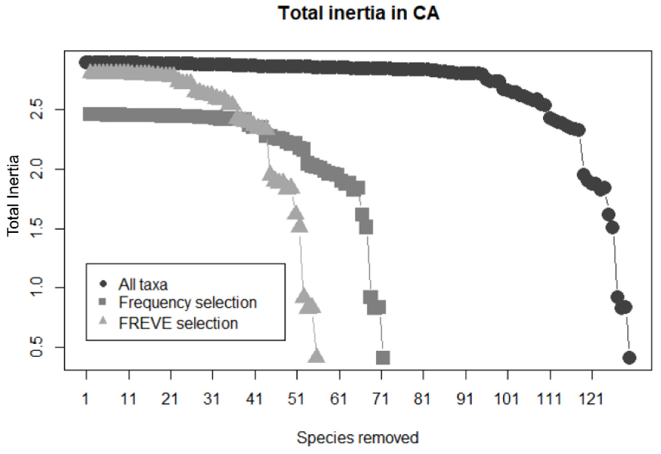
A comparison between selection methods was made using Inertia Analysis. Total Inertia (TI) was calculated as the sum of the eigenvalues of the χ² dissimilarity matrix. Taxa were sequentially removed from less abundant to abundant and TI was recalculated (Figure 4). The initial TI’s value of the complete dataset (2.89) is closer to the TI value for the dataset obtained by FREVE selection (2.81) than the TI values obtained by frequency selection (2.46). This means that FREVE retains more information from the original dataset. The one species rescued by FREVE (Table 1) was responsible for about 13% of the data TI, more than the 17 discarded taxa.

3.2. Evaluation of n-Partition

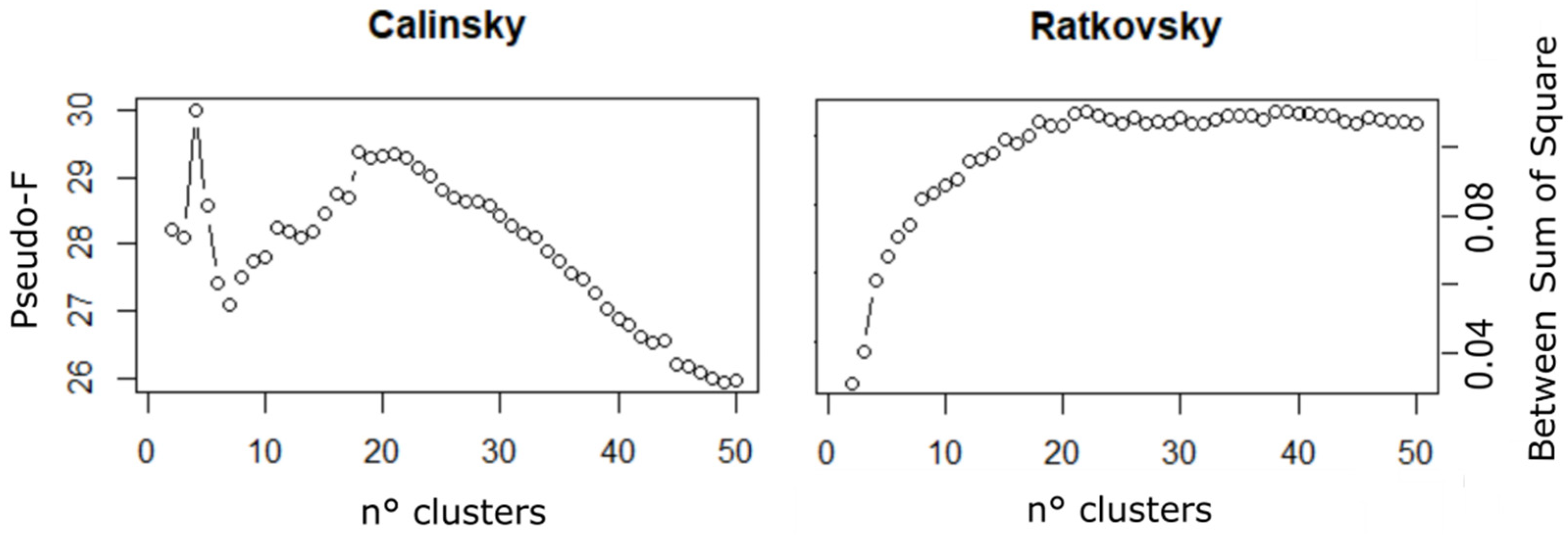
Among all possible partitions, the Calinski pseudo-F values peaked for the partition with four clusters and reached a second maximum for the partition with 18 clusters (Figure 5, left). The Ratkowsky Between-Sum-of-square increase rate was highest between partitions with three and four clusters (Figure 5, right), indicating that the best number of clusters was four. Between 18 and 20 clusters, the Ratkowsky’s index reached the plateau. Finally, two partitions with 4 and 18 clusters were chosen to obtain a broad and a fine resolution in the data discontinuities, respectively.

3.3. Original Protocol Temporal Map

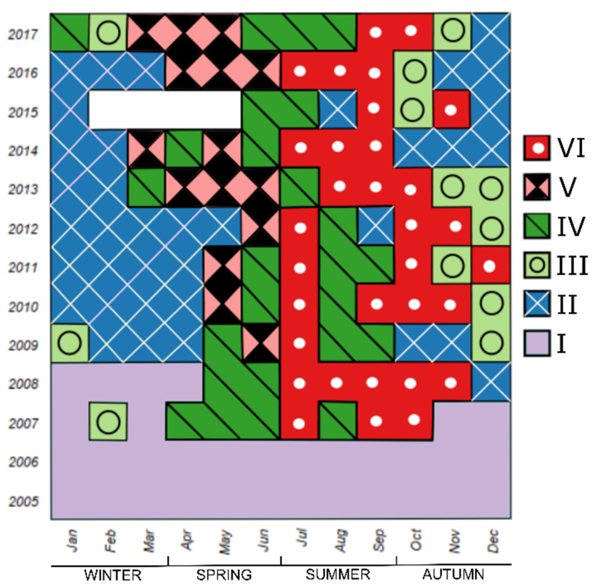
For the temporal map obtained with the original protocol (Figure 2A), the best of possible partitions with six clusters were used and the IndVal index was applied to select the indicative taxa of the clusters (Figure 6). A total of 43 out of 73 taxa were found to be indicative of at least one cluster (

Table 2. Composition of taxa in clusters derived from the original protocol sensu Anneville et al., (2002) with corresponding IndVal value. Only taxa with IndVal value higher than 0.25 are shown. The taxa are organized in descending order of IndVal value.

Cluster	Taxon	IndVal	Cluster	Taxon	IndVal
I	/	/	V	Cyclotella spp.	0.46
II	Skeletonema costatum s.l.	0.33		Prorocentrum compressum	0.44
	Ophiaster hydroideus	0.26		Euglenophyceae	0.42
III	Eucampia spp.	0.80		Bacteriastrum delicatulum	0.42
	Pseudo-nitzschia seriata gr.	0.62		Prorocentrum balticum	0.40
	Lauderia annulata	0.62		Prorocentrum micans	0.39
	Calciosolenia murrayi	0.61		Prasinophyceae	0.38
	Pleurosigma normanii	0.54		Prorocentrum cordatum	0.33
	Cylindrotheca closterium	0.53		Alexandrium minutum	0.32
	Asterionellopsis glacialis	0.50		Diatoms non ident.	0.31
	Leptocylindrus mediterraneus	0.49		Leptocylindrus danicus	0.29
	Thalassiosira spp.	0.43		Nitzschia longissima	0.29
	Chaetoceros spp.	0.43		Cryptophyceae	0.29
	Nitzschia spp.	0.43		Gymnodinium spp.	0.29
	Proboscia indica	0.41		Prorocentrum triestinum	0.28
	Cerataulina pelagica	0.37		Amphora spp.	0.28
	Pseudo-nitzschia delicatissima gr.	0.37	VI	Rhizosolenia spp.	0.54
	Leptocylindrus danicus	0.34		Proboscia alata	0.53
	Emiliania huxleyi	0.32		Rhabdosphaera stylifera	0.51
	Guinardia flaccida	0.31		Pseudo-nitzschia delicatissima gr.	0.49
	Thalassionema nitzschioides	0.28		Dactyliosolen fragilissimus	0.40
IV	Cyclotella spp.	0.29		Syracosphaera pulchra	0.37
	Cerataulina pelagica	0.25		Thalassionema nitzschioides	0.34
V	Calyptrosphaera oblonga	0.63		Hemiaulas hauckii	0.29
	Heterocapsa gr.	0.49		Tripos fusus	0.29
	Chlorophyceae	0.46		Guinardia striata	0.28

). The cluster map revealed a rough seasonal pattern except for the first two years (2005 and 2006). These two years and parts of 2007 and 2008 belonged entirely to Cluster I, in which no taxa exceeded the threshold (IndVal = 0.25) to be defined as indicative. From 2009 onwards, the winter (January–March) was mostly characterized by Cluster II with two indicative species, the diatom Skeletonema costatum s.l. and the coccolithophore Ophiaster hydroideus. In 2009–2012, Cluster II extended into spring, whereas in recent years, it had already appeared in autumn. Cluster III almost always appeared before Cluster II, usually in autumn (October to December). This cluster was described by many indicative taxa, predominantly diatoms. Seven taxa had IndVal > 0.5: the diatoms Asterionellopsis glacialis, Cylindrotheca closterium, Eucampia spp., Lauderia annulata, Pleurosigma normanii and the Pseudo-nitzschia seriata group, as well as a coccolithophore Calciosolenia murrayi. Cluster III was generally anticipated by Cluster VI, typical of the summer (July to September) and occasionally extended into the autumn, which contained ten indicative taxa, mostly diatoms. Three taxa had IndVal > 0.5: the diatoms Proboscia alata and Rhizosolenia spp. and a coccolithophore Rhabdosphaera stylifera. Cluster IV was intermittently present in spring and summer and best described the temporal distribution for two diatom taxa: Cyclotella spp. and Cerataulina pelagica. Finally, Cluster V appeared in 2009 and characterized the spring from March to June. Cluster V was represented by a mixed phytoplankton community, but only one coccolithophore (Calyptrosphaera oblonga) had IndVal > 0.5.

Five taxa were indicative of more than one cluster. Excluding the first two years, the typical sequence of phytoplankton during the study period was Cluster II—Cluster V—Cluster IV—Cluster VI—Cluster III.

3.4. Modified Protocol Temporal Map

3.4.1. Four-Clustered Partition

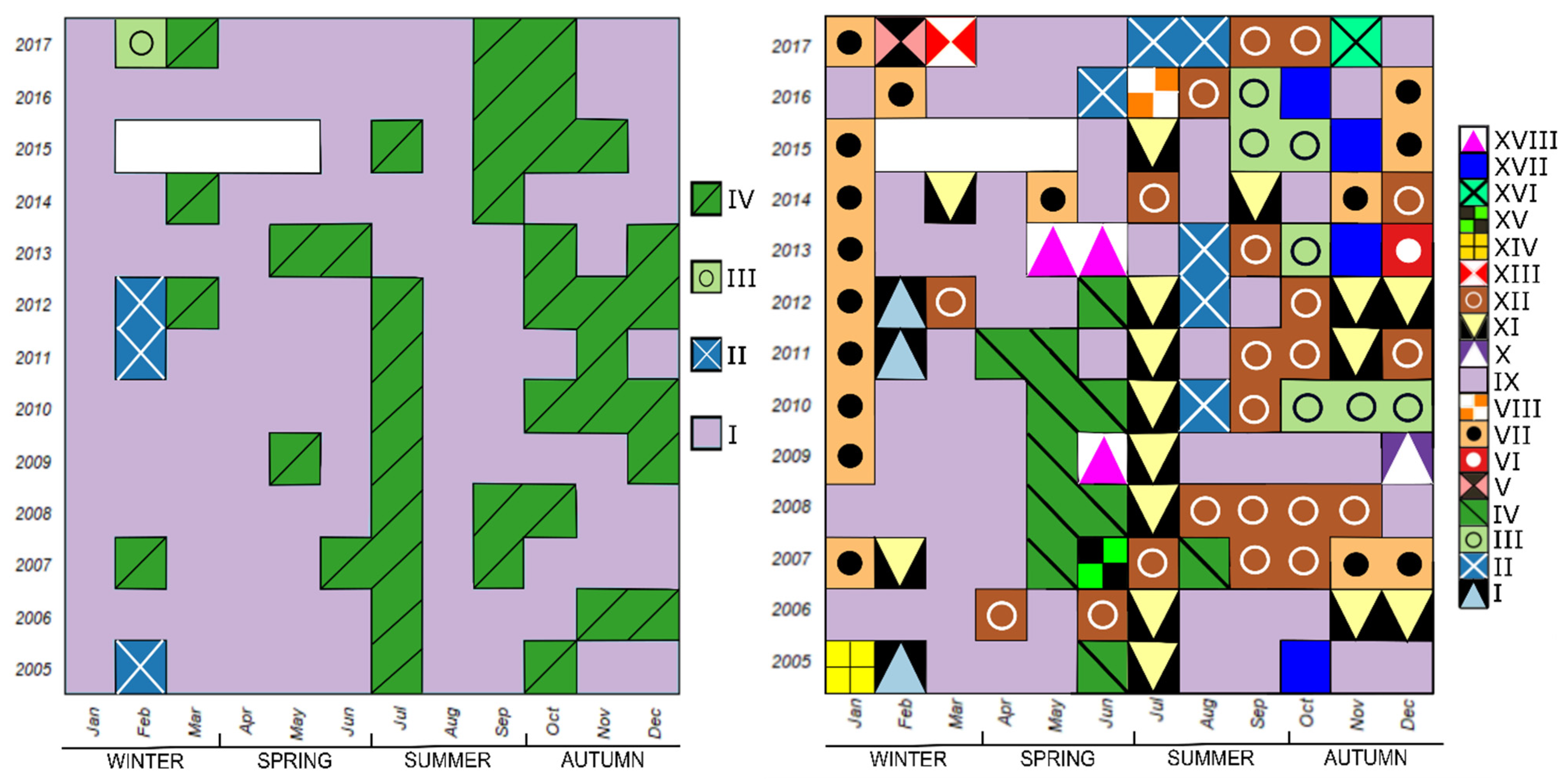
The temporal map showing four clusters obtained with the modified protocol (Figure 2B) is shown in Figure 7 (left), while indicative taxa with Xproj and IndVal values for these clusters are summarized in

Table 3. Taxa composition of the 4-clustered partition with corresponding Likelihood ratios (Xproj) for the centroids and IndVal values (IndVal). Taxa with Xproj > 1 or IndVal value > 0.25 are shown in bold. Taxa in both columns are organized in descending order of IndVal and Xproj. The term “Nanoflagellates” stands for flagellates in the nanoplankton size fraction that have not been identified as prasinophytes, cryptophytes, etc.

Cluster	Taxon (Ranked by Xproj)	Xproj	Taxon (Ranked by IndVal)	IndVal
I	Meringosphaera mediterranea	0.78	Prasinophyceae	0.42
	Diploneis crabro	0.68	Diatoms non ident.	0.41
	Diatoms non ident.	0.61	Meringosphaera mediterranea	0.39
	Cylindrotheca Closterium	0.56	Diploneis crabro	0.36
	Ophiaster hydroideus	0.53	Cryptophyceae	0.33
	Emiliania huxleyi	0.48	Cylindrotheca closterium	0.33
	Cryptophyceae	0.44	Heterocapsa gr.	0.3
	Dictyocha fibula	0.41	Cyclotella spp.	0.29
	Prorocentrum cordatum	0.39	nanoflagellates	0.29
	Nanoflagellates	0.37	Ophiaster hydroideus	0.26
	Gonyaulax spp.	0.37	Emiliania huxleyi	0.26
II	Skeletonema costatum s.l.	22.00	Skeletonema costatum s.l.	0.98
	Chaetoceros simplex	5.23	Chaetoceros simplex	0.55
	Prorocentrum compressum	−0.25	Emiliania huxleyi	0.29
	Scrippsiella trochoidea	−0.25	Scrippsiella trochoidea	0.28
III	Chaetoceros curvisetus	76.01	Chaetoceros curvisetus	1
	Leptocylindrus danicus	9.61	Leptocylindrus danicus	0.87
	Lauderia annulata	4.33	Prorocentrum micans	0.75
	Prorocentrum compressum	2.92	Lauderia annulata	0.75
	Asterionellopsis glacialis	2.85	Asterionellopsis glacialis	0.68
	Prorocentrum micans	2.51	Prorocentrum compressum	0.66
	Prorocentrum cordatum	2.22	Prorocentrum cordatum	0.66
	Prorocentrum balticum	1.68	Prorocentrum balticum	0.64
	Bacteriastrum delicatulum	1.42	Bacteriastrum delicatulum	0.58
	Hemiaulas hauckii	1.26	Hemiaulas hauckii	0.56
	Nitzschia longissima	0.4	Nitzschia longissima	0.53
	Pleurosigma normanii	0.2	Dictyocha fibula	0.52
	Prorocentrum triestinum	0.19	Prorocentrum triestinum	0.47
	Guinardia striata	0.15	Pleurosigma normanii	0.44
	Dictyocha fibula	0.11	Prorocentrum gracile	0.39
	Pseudo-nitzschia seriata gr.	−0.08	Guinardia striata	0.38
	Cerataulina pelagica	−0.13	Cyclotella spp.	0.37
	Prorocentrum gracile	−0.27	Pseudo-nitzschia seriata gr.	0.32
	Gyrodinium. spp.	−0.27	Gyrodinium spp.	0.32
	Cyclotella spp.	−0.37	Cerataulina pelagica	0.31
	Thalassionema nitzschioides	−0.37	Thalassionema nitzschioides	0.3
	Rhizosolenia spp.	−0.38	Rhizosolenia spp.	0.25
IV	Lauderia annulata	2.17	Pseudo-nitzschia delicatissima gr.	0.86
	Asterionellopsis glacialis	1.38	Chaetoceros spp.	0.81
	Guinardia striata	1.34	Proboscia alata	0.79
	Leptocylindrus mediterraneus	1.18	Dactyliosolen fragilissimus	0.64
	Pseudo-nitzschia seriata gr.	1.08	Nitzschia spp.	0.6
	Bacteriastrum delicatulum	1.05	Cerataulina pelagica	0.6
	Chaetoceros spp.	0.92	Syracosphaera pulchra	0.55
	Cerataulina pelagica	0.8	Euglenophyceae	0.54
	Pleurosigma normanii	0.76	Rhizosolenia spp.	0.49
	Rhabdosphaera stylifera	0.75	Rhabdosphaera stylifera	0.46
	Dactyliosolen fragilissimus	0.75	Tripos fusus	0.44
	Hemiaulas hauckii	0.7	Pseudo-nitzschia seriata gr.	0.41
	Leptocylindrus danicus	0.67	Guinardia flaccida	0.41
	Guinardia flaccida	0.59	Heterocapsa gr.	0.41
	Coccolith. non ident.	0.59	Cylindrotheca closterium	0.41
	Pseudo-nitzschia delicatissima gr.	0.59	Leptocylindrus mediterraneus	0.39
	Proboscia alata	0.55	Prasinophyceae	0.39
	Syracosphaera pulchra	0.49	Calciosolenia murrayi	0.38
	Thalassiosira spp.	0.49	Thalassionema nitzschioides	0.37
	Tripos fusus	0.35	Guinardia striata	0.36
	Calciosolenia murrayi	0.3	Diploneis crabro	0.35
	Rhizosolenia spp.	0.3	Thalassiosira spp.	0.34
	Euglenophyceae	0.28	Gymnodinium spp.	0.32
	Nitzschia longissima	0.21	nanoflagellates	0.3
	Prorocentrum triestinum	0.21	Calciosolenia brasiliensis	0.29
	Dinobryon spp.	0.18	Ophiaster hydroideus	0.26
	Oxytoxum spp.	0.1	Pleurosigma normanii	0.26
	Protoperidinium spp.	0.08	Diatoms non ident.	0.26
	Calciosolenia brasiliensis	0.05	Cryptophyceae	0.25
	Nitzschia spp.	0.04	Emiliania huxleyi	0.25

. Two clusters showed some degree of seasonality. The “winter” Cluster II was strongly associated with the diatoms Skeletonema costatum s.l. and Chaetoceros simplex (Xproj 22.0 and 5.23, respectively, and IndVal > 0.5), but was restricted to February 2005, 2011, and 2012. The “summer and autumn” Cluster IV, which was also occurred sporadically in the early spring, was indicative of diatom blooms. Six diatom taxa had a meaningful Xproj > 1 for this cluster, while a variety of other taxa in a different order (though mainly diatoms) were indicated as typical by IndVal ≥ 0.25. Interestingly, the centroid of the Cluster IV was most associated with Lauderia annulata, which had IndVal < 0.25. Cluster III was present only in February 2017 and was associated with the diatoms Chaetoceros curvisetus, Leptocylindrus danicus and L. annulata. The largest of the clusters, Cluster I, was distributed across all other months and represented the mixed phytoplankton community of nanoflagellates, small diatoms and some coccolithophore taxa, although none of the Xproj or IndVal were particularly high. The Mantel test between the two ordination indices (Xproj and IndVal) showed a significant correlation (r = 0.78; p-value = 0.03).

3.4.2. Eighteen-Clustered Partition

The temporal map of 18 clusters obtained with the modified protocol is shown in Figure 7 (right), with the corresponding Xproj and IndVal values summarized in

Table 4. Taxa composition of the 18-clustered partition with corresponding Likelihood ratios (Xproj) for the centroids and IndVal values (IndVal). Taxa with Xproj > 1 or IndVal > 0.25 are in bold. Taxa in both columns are organized in descending order of IndVal and Xproj. The term “Nanoflagellates” stands for flagellates in the nanoplankton size fraction that have not been identified as prasinophytes, cryptophytes, etc.

Cluster	Taxon (Ranked by Xproj)	Xproj	Taxon (Ranked by IndVal)	IndVal
I	Skeletonema costatum s.l.	22.0	Skeletonema costatum s.l.	0.92
	Chaetoceros simplex	5.23	Chaetoceros simplex	0.23
II	Diatoms non ident.	10.1	Diatoms non ident.	0.38
	Guinardia flaccida	5.01	Dactyliosolen fragilissimus	0.18
	Dactyliosolen fragilissimus	4.20	Heterocapsa gr.	0.12
	Prorocentrum triestinum	4.12	Prorocentrum triestinum	0.12
	Oxytoxum spp.	1.82	Chlorophyceae	0.11
	Heterocapsa gr.	1.69	Guinardia flaccida	0.10
	Pleurosigma normanii	1.58	Cyclotella spp.	0.07
	Prorocentrum gracile	1.49	Thalassionema nitzschioides	0.06
	Guinardia striata	1.17	Prorocentrum balticum	0.06
	Chlorophyceae	1.16	Gyrodinium spp.	0.06
	Thalassionema nitzschioides	1.14	Prorocentrum gracile	0.06
	Hemiaulas hauckii	1.07	Cryptophyceae	0.06
III	Calciosolenia murrayi	4.75	Pseudo-nitzschia delicatissima gr.	0.65
	Pseudo-nitzschia delicatissima gr.	4.37	Nitzschia spp.	0.28
	Syracosphaera pulchra	2.11	Syracosphaera pulchra	0.28
	Tripos fusus	1.87	Calciosolenia murrayi	0.24
	Dactyliosolen fragilissimus	1.63	Dactyliosolen fragilissimus	0.20
	Tripos furca	1.59	Gyrodinium spp.	0.18
	Calciosolenia brasiliensis	1.55	Tripos fusus	0.18
	Nitzschia spp.	1.39	Calciosolenia brasiliensis	0.17
	Prorocentrum triestinum	1.24	Ophiaster hydroideus	0.16
	Rhabdosphaera stylifera	1.12	Rhizosolenia spp.	0.13
	Gyrodinium spp.	1.12	Tripos furca	0.13
	Leptocylindrus mediterraneus	1.09	Pseudo-nitzschia seriata gr.	0.11
IV	Cyclotella spp.	5.28	Cyclotella spp.	0.44
	Chaetoceros simplex	4.02	Prorocentrum gracile	0.20
	Prorocentrum gracile	2.97	Prorocentrum cordatum	0.13
	Heterocapsa gr.	1.08	Chaetoceros simplex	0.13
	Prorocentrum cordatum	1.03	Prasinophyceae	0.12
V	Chaetoceros curvisetus	76.0	Chaetoceros curvisetus	0.95
	Leptocylindrus danicus	9.61	Prorocentrum cordatum	0.31
	Lauderia annulata	4.33	Prorocentrum balticum	0.24
	Prorocentrum compressum	2.92	Leptocylindrus danicus	0.23
	Asterionellopsis glacialis	2.85	Hemiaulas hauckii	0.22
	Prorocentrum micans	2.51	Prorocentrum micans	0.21
	Prorocentrum cordatum	2.22	Prorocentrum compressum	0.20
	Prorocentrum balticum	1.68	Bacteriastrum delicatulum	0.12
	Bacteriastrum delicatulum	1.42	Guinardia striata	0.11
	Hemiaulas hauckii	1.26	Nitzschia longissima	0.11
VI	Lauderia annulata	114.	Lauderia annulata	0.83
	Leptocylindrus mediterraneus	22.7	Leptocylindrus mediterraneus	0.54
	Thalassiosira spp.	7.94	Thalassiosira spp.	0.28
	Guinardia flaccida	5.54	Gonyaulax spp.	0.20
	Cerataulina pelagica	4.35	Guinardia flaccida	0.18
	Leptocylindrus danicus	2.89	Protoperidinium spp.	0.12
	Thalassionema nitzschioides	2.03	Thalassionema nitzschioides	0.10
	Gonyaulax spp.	1.76	Calciosolenia brasiliensis	0.08
	Protoperidinium spp.	1.63	Ophiaster hydroideus	0.08
	Calciosolenia brasiliensis	1.35	Pleurosigma normanii	0.08
	Pleurosigma normanii	1.34	Dactyliosolen fragilissimus	0.08
	Nitzschia longissima	1.01	Gyrodinium spp.	0.07
VII	Emiliania huxleyi	3.71	Emiliania huxleyi	0.11
	Ophiaster hydroideus	1.74	Ophiaster hydroideus	0.07
	Diploneis crabro	1.73	Diploneis crabro	0.07
	Gonyaulax spp.	1.66	Prasinophyceae	0.06
	Cylindrotheca closterium	1.24	Meringosphaera mediterranea	0.06
VIII	Dictyocha fibula	97.2	Dictyocha fibula	0.92
	Rhabdosphaera stylifera	10.2	Rhabdosphaera stylifera	0.54
	Oxytoxum spp.	10.1	Oxytoxum spp.	0.44
	Calciosolenia brasiliensis	5.17	Calciosolenia brasiliensis	0.27
	Prorocentrum micans	4.36	Tripos furca	0.20
	Prorocentrum triestinum	4.14	Prorocentrum triestinum	0.18
	Diatoms non ident.	3.04	Diatoms non ident.	0.18
	Diploneis crabro	2.90	Prorocentrum micans	0.17
	Prorocentrum compressum	2.71	Diploneis crabro	0.17
	Tripos furca	2.53	Heterocapsa gr.	0.14
	Thalassionema nitzschioides	2.25	Scrippsiella trochoidea	0.14
	Scrippsiella trochoidea	2.20	Thalassionema nitzschioides	0.13
	Heterocapsa gr.	1.85	Chlorophyceae	0.12
	Cylindrotheca closterium	1.10	Prorocentrum compressum	0.10
IX	Meringosphaera mediterranea	1.05	Cryptophyceae	0.08
X	Asterionellopsis glacialis	61.3	Asterionellopsis glacialis	0.79
	Lauderia annulata	3.51	Ophiaster hydroideus	0.21
	Thalassiosira spp.	2.66	Thalassiosira spp.	0.16
	Cerataulina pelagica	2.63	Guinardia striata	0.13
	Ophiaster hydroideus	2.14	Thalassionema nitzschioides	0.13
	Leptocylindrus mediterraneus	1.98	Leptocylindrus mediterraneus	0.10
	Thalassionema nitzschioides	1.69	Diploneis crabro	0.09
	Guinardia striata	1.21	Calciosolenia murrayi	0.09
	Calciosolenia murrayi	1.21	Cerataulina pelagica	0.07
XI	Chaetoceros spp.	2.53	Proboscia alata	0.45
	Proboscia alata	1.78	Chaetoceros spp.	0.38
XII	Coccolith. non ident.	4.43	Nitzschia spp.	0.14
	Guinardia striata	2.50	Guinardia striata	0.12
	Oxytoxum spp.	1.78	Dactyliosolen fragilissimus	0.10
	Hemiaulas hauckii	1.68	Syracosphaera pulchra	0.09
	Dactyliosolen fragilissimus	1.48	Hemiaulas hauckii	0.09
	Rhabdosphaera stylifera	1.27	Coccolith. non ident.	0.09
	Nitzschia spp.	1.14	Proboscia alata	0.07
	Pleurosigma normanii	1.05	Rhabdosphaera stylifera	0.06
XIII	Dinobryon spp.	39.1	Dinobryon spp.	0.84
	Leptocylindrus danicus	19.9	Leptocylindrus danicus	0.46
	Prorocentrum compressum	5.51	Prorocentrum compressum	0.34
	Chaetoceros curvisetus	2.45	Scrippsiella trochoidea	0.28
	Prorocentrum micans	2.40	Prorocentrum micans	0.21
	Scrippsiella trochoidea	2.35	Nitzschia longissima	0.18
	Nitzschia longissima	1.35	Prasinophyceae	0.18
XIV	Emiliania huxleyi	17.2	Emiliania huxleyi	0.41
	Dinobryon spp.	16.2	Meringosphaera mediterranea	0.30
	Prorocentrum gracile	6.36	Prorocentrum gracile	0.21
	Meringosphaera mediterranea	5.11	Diploneis crabro	0.17
	Diploneis crabro	4.91	Dinobryon spp.	0.12
	Protoperidinium spp.	2.33	Protoperidinium spp.	0.12
	Chaetoceros simplex	1.16	Chaetoceros simplex	0.07
	Calciosolenia murrayi	1.01	Calciosolenia murrayi	0.05
XV	Cerataulina pelagica	20.7	Cerataulina pelagica	0.65
	Leptocylindrus danicus	7.56	Guinardia flaccida	0.26
	Guinardia flaccida	3.12	Tripos furca	0.19
XVI	Cylindrotheca closterium	30.7	Cylindrotheca closterium	0.53
	Calciosolenia murrayi	11.9	Calciosolenia murrayi	0.26
	Pleurosigma normanii	9.42	Pleurosigma normanii	0.26
	Nitzschia longissima	6.55	Nitzschia longissima	0.18
	Thalassionema nitzschioides	5.11	Ophiaster hydroideus	0.14
	Ophiaster hydroideus	3.36	Thalassionema nitzschioides	0.14
	Calciosolenia brasiliensis	2.62	Tripos fusus	0.09
	Diploneis crabro	2.56	Calciosolenia brasiliensis	0.09
	Tripos fusus	1.80	Diploneis crabro	0.09
	Diatoms non ident.	1.55	Syracosphaera pulchra	0.08
	Guinardia flaccida	1.41	Nitzschia spp.	0.08
	Syracosphaera pulchra	1.20	Meringosphaera mediterranea	0.07
	Nitzschia spp.	1.17	Diatoms non ident.	0.06
	Asterionellopsis glacialis	1.10	Guinardia striata	0.06
	Chaetoceros curvisetus	1.07	Gyrodinium spp.	0.05
XVII	Pseudo-nitzschia seriata gr.	15.8	Pseudo-nitzschia seriata gr.	0.62
	Protoperidinium spp.	5.80	Protoperidinium spp.	0.29
	Asterionellopsis glacialis	4.03	Thalassiosira spp.	0.25
	Nitzschia longissima	3.72	Guinardia striata	0.13
	Pleurosigma normanii	2.98	Syracosphaera pulchra	0.10
	Thalassiosira spp.	2.57	Dactyliosolen fragilissimus	0.09
	Cylindrotheca closterium	2.10	Nitzschia longissima	0.09
	Prorocentrum triestinum	2.00	Pleurosigma normanii	0.09
	Calciosolenia murrayi	1.57	Nitzschia spp.	0.09
	Diploneis crabro	1.35	Calciosolenia murrayi	0.08
	Guinardia striata	1.27	Chaetoceros spp.	0.08
	Oxytoxum spp.	1.11	Asterionellopsis glacialis	0.07
XVIII	Bacteriastrum delicatulum	21.4	Bacteriastrum delicatulum	0.67
	Prorocentrum micans	4.60	Euglenophyceae	0.26
	Prorocentrum compressum	2.85	Heterocapsa gr.	0.24
	Heterocapsa gr.	2.52	Prorocentrum balticum	0.18
	Euglenophyceae	2.30	Prorocentrum micans	0.17
	Prorocentrum balticum	2.21	Prorocentrum triestinum	0.13
	Prorocentrum gracile	1.90	Prorocentrum compressum	0.12
	Prorocentrum triestinum	1.74	Scrippsiella trochoidea	0.11
	Oxytoxum spp.	1.28	Cyclotella spp.	0.10
	Scrippsiella trochoidea	1.04	Chlorophyceae	0.10

. It shows a more complex picture of seasonality, especially in autumn. Ten clusters included three or more samples/months, while the remaining eight included only one sample/month.

During winter, the most important clusters were Cluster VII, strongly associated with the coccolithophore Emiliania huxleyi, and Cluster IX associated with the chrysophycean species Meringosphaera mediterranea. Cluster IX was also scattered in the other seasons.

In spring, the main clusters were IV and XVIII. From 2005 to 2012, late spring was characterized by Cluster IV associated with the diatoms Cyclotella spp. and C. simplex and the dinoflagellates Prorocentrum gracile, Prorocentrum cordatum and the Heterocapsa group. In 2009 and 2013, another late spring cluster (Cluster XVIII) formed, most strongly associated with the diatom Bacteriastrum delicatulum, as well as dinoflagellates from the genus Prorocentrum, the coccolitophore Calyptrosphaera oblonga, and undetermined euglenophytes.

The most important summer cluster, typical mainly of July during 2005–2012, was Cluster XI, which was also sporadically present in other seasons, especially in late autumn. This cluster was associated with the diatoms Chaetoceros spp. and Proboscia alata. From 2010, another summer cluster (Cluster II) appeared, characterized by a diverse community of diatoms (e.g., Guinardia flaccida, Dactyliosolen fragilissimus and undetermined species), dinoflagellates (e.g., Prorocentrum triestinum, P. gracile) and chlorophytes.

Autumn months were the most varied and richest for the occurrence of various clusters. Besides scattered occurrences of Cluster IX and Cluster XI, this season was characterized by three clusters: Cluster XII, Cluster III and Cluster XVII. Cluster XII was most typical in October and November and was associated with undetermined coccolithophores and various diatoms such as Guinardia striata, Hemiaulus hauckii and D. fragilissimus. From 2010, the Cluster III appeared, associated with coccolithophores Calciosolenia murrayi and Syracosphaera pulchra, diatoms from the Pseudo-nitzschia delicatissima group and some dinoflagellates. Finally, Cluster XVII was associated with diatoms such as species from Pseudo-nitzschia seriata group, Asterionellopsis glacialis, Nitzschia longissima and Pleurosigma normanii.

A correlation of 0.87 with p-value = 0.001 was obtained between the two ordination indices (Xproj and IndVal).

4. Discussion

4.1. Review of the Critical Steps of Analysis

4.1.1. Taxa Selection, Ordination and Clustering

Plankton communities have complex and dynamic structure [40]. To unveil the temporal patterns of these communities it is often necessary to reduce the number of variates (i.e., taxa); however, preserving a representative amount of information is key when choosing different methods of taxa selection. Our results show that Total Inertia (TI), which was used as an indicator of the total amount of information present in the dataset [36] was higher when FREVE was used compared to the selection based on frequency of appearance. In other words, FREVE was more effective in preserving information (Figure 4). In the “real life” scenario of the GoT coastal ecosystem, the four distribution types we postulate can be interpreted as follows: Type 1 taxa can be considered occasional, e.g., only occasionally driven by currents or otherwise introduced; Type 2 taxa are also infrequent but may reproduce and bloom under favourable conditions; Type 3 taxa are common and bloom regularly; and Type 4 taxa are commonly present but always with low abundances. For the interpretation of phenology of the phytoplankton typical of the basin, the taxa of types 2 and 3 seemed to be more interesting because they contribute to the seasonal dynamics more than taxa of types 1 and 4. However, because taxa of type 4 are common, helping to define the baseline of the community and tending to structure the abundance matrix, the objective was then to eliminate only taxa of type 1 from the dataset. Taxa of types 1 and 4 share a common feature: in the samples in which they were present, they exhibited constant or quasi-constant abundance and are therefore found near or on the log distribution (Figure 3A). Taxa of types 2 and 3 also share a common feature: they exhibited fluctuating abundance in the samples in which they were present, so that the majority of abundance is concentrated in only a fraction of the samples. Considering again the FREVE index, instead of evenness we could have chosen dominance indices (like Simpson), which are invariant across the number of classes [41] but we were more interested in evaluating the space occupied by the classes (samples) over the disposable space (the whole time series). Moreover, Pielou’s characteristic of variation between 0 and 1 made it ideal for coupling with frequency compared to other entropy indices.

The differences between temporal maps obtained by PCA (Figure 6) and CA (Figure 7) cannot be associated only with the selected number of clusters in which to divide the matrix (6 clusters vs. 4 clusters or 18 clusters) or the different taxa selection methods used in the two protocols, but they mostly express a qualitative difference between the two types of analysis. Legendre and Legendre [36] argue that Euclidean distance on which PCA relies is not a good distance method for studying species frequency tables because of the double-zero problem. We detected an increase in diversity over the years using Pielou’s evenness index (data not shown). This increase could be due to a real increase in diversity or to better taxonomical skills of the expert who analysed the samples. Regardless of the reason, we observed a concentration of presences inside fewer taxa in the first years of the data series, which also means a high number of zero or near zero abundance values for other taxa. The large cluster covering the first years (2005–2006) of the series (see Cluster I in Figure 6) with no seasonal structure and no indicative taxa was indeed the dataset region that contained most of the zeros.

With the use of a more adequate ordination method, i.e., CA that resulted in temporal maps in which diverse seasonal clusters were observed throughout the data series (Figure 7), we also confirmed the existence of seasonal patterns of phytoplankton community during the first years. The seasonality of the clusters was found in both partition levels (4 and 18) for this first part of the temporal series. The main difference between the two was that the 4-clustered and 18-clustered partitioning levels allowed us to observe seasonal patterns at two different degrees of complexity: a baseline structure of the phytoplankton community in the Gulf of Trieste (Figure 7, left) and a more detailed one (Figure 7, right), which will be further discussed.

As regards the clustering algorithm, we consider the method based on k-means clustering better than the method based on Bayes’ rule proposed in the original protocol. Bayes’ rule forces the clusters to achieve an equilibrium between dimension and homogeneity, but this would come at the cost of cutting off part of the complexity of the matrix. With the k-means method, the clusters are not weighted according to their relative dimension but only based on the fraction of variance that they explain. Thus, when using the k-means method, blooming events can form small outlying clusters easier than using Bayes’ rule. Moreover, the k-means algorithm dictates the use of multiple random starts to avoid local maxima in the objective function, a problem that is not tackled in the original protocol. Finally, the use of the Calinski pseudo-F and Ratkowsky indices, which are both based on the analysis of variance, is preferable to the use of the probability vector ${\mathrm{P}}_{\max }\left(\mathrm{k}\right)$ proposed in the original protocol. This is for the same reason that the k-means method is preferable to Bayes’ rule.

4.1.2. Indicative Taxa

Characterization of the indicative species of clusters using the IndVal index resulted in some taxa that were indicative of more than one cluster. Examples include Cyclotella sp. in Clusters IV and V of the original protocol (IndVal 0.29 and 0.46, Table 2) and Emiliania huxleyi in Clusters I, II and IV of the modified protocol (IndVal 0.26, 0.29 and 0.25, Table 3). The fact that “IndVal removes any effect of the number of the sites in the various clusters and also differences in abundance among sites belonging to the cluster” [34] was in some cases a serious flaw of the method. Both the taxa in the example (Cyclotella sp. and Emiliania huxleyi) are very common in the phytoplankton community and consequently the fidelity term (Equation (1)) of the IndVal formula (Equation (3)) is, for many of the possible cluster, close to $1$. The other term (Equation (2)), known as specificity, should counterbalance this by giving more weight to clusters that contain most of the average taxon’s abundance. However, it is possible that the average abundance is quasi-constant between clusters, in particular when the clusters describe taxa distribution sub-optimally, which is often the case when the number of taxa is high while the number of clusters is low [36].

Another example of an IndVal computational flaw is given by the single-sample Cluster III (Table 3) and the corresponding Cluster V (Table 4). Those two clusters belong to two different partitioning levels of the same taxa selection (modified protocol) and were both indicative only for February 2017. However, they exhibit different species selection with high IndVal values. While more than 20 taxa were indicative of Cluster III of the 4-clustered partition, only two were indicative of Cluster V of the 18-clustered partition. This is explained by the way in which the IndVal index is calculated in both cases. The fidelity term for the taxa present in February 2017 is, in both cases, equal to $1$ (Equation (1)). Instead, the denominator ${\mathrm{NI}}_{+\mathrm{j}}$ (Equation (2)) of the specificity term varies since it is the sum of the mean abundances of all clusters [34]. With further refining in the 18-clustered partition and the division of big clusters from the 4-clustered partition into smaller clusters, the abundance peaks of more taxa were better defined by some of these smaller clusters. Consequently, the denominator ${\mathrm{NI}}_{+\mathrm{j}}$ (Equation (2)) increased, the specificity term dropped, and many taxa were no longer defined as indicative for February 2017, despite the fact that the cluster remained unchanged.

The likelihood ratio method (Xproj—Appendix B) served as a supplementary estimator of indicative taxa for a cluster because the arbitrary threshold (0.25) of the IndVal index was ambiguous. K-means clustering minimizes the within-cluster variance [36] which being expressed in ${\mathsf{\chi }}^2$ metric tends to separate similarly deviant samples from average profile samples [36]. In this way, the taxa with higher likelihood ratios are those most responsible for the formation of deviant clusters, while taxa with likelihood values close to zero are responsible for large average clusters. The likelihood ratios $\left(\mathrm{Observed}/\mathrm{Expected}\right)$ present an advantage because they are not constrained between $0$ and $1,$ which allows more precise identification of the taxa that are most important for the definition of a cluster. Below zero Xproj values indicate taxa that were present less than expected in a cluster and they also play a role in the definition of clusters. The single-sampled cluster of February 2017 can again serve as a good example. Two diatom species, Chaetoceros curivesetus and Leptocylindrus danicus, had similarly high IndVal values for Cluster III in 4-clustered partition (1 and 0.87, respectively, Table 3), which reveals that both are strongly indicative of this cluster. On the other hand, Xproj results show a substantial difference between the importances of the two species: in February 2017, the abundance of C. curivesetus was more than 70 times higher than expected (Xproj 76.0), while it was just ten times higher than expected for L. danicus (Xproj 9.61). Another important advantage of (Xproj) values is that the value for a taxon does not change between the different n-clustered partitions as long the centroid of the cluster remains the same (e.g., Cluster III in Table 3 and Cluster V in Table 4). As stated in the definition of methods, the deviation values (Xproj) are dependent only on the centroid of a cluster, which in this case is the same for both clusters (Appendix B).

Although the two indexing systems (IndVal and Xproj) have organized the indicative taxa in a similar way (as shown by highly significant correlation), substantial advantages have emerged for Xproj suggesting it as a preferred option in defining indicative taxa.

In summary, from an analytical point of view, for a correct representation of the assemblages we recommend to use (i) non log-transformed data, (ii) a selection method that preserves the information (like FREVE), (iii) distances that are not sensitive to the double-zero problem (such as the chi-square distance), (iv) a clustering method that minimizes the variance within clusters (such as k-means), and (v) more indices to define indicative taxa (the pair IndVal and Xproj seems effective).

4.2. Phytoplankton Phenology in the Period 2005–2017

In the 4-clustered partition (Figure 7, left), the main distinction that can be made between clusters represent two phytoplankton communities which are known to occur under different environmental conditions in the Gulf of Trieste [40]. In fact, the largest Cluster I is indicative of a mixed community composed mainly of nanoflagellates, diatoms and coccolithophores, while the remaining clusters (II, III and IV) represent the period of the year when diatom abundances increase and dominate the community. This alternation between the dominance of different phytoplankton groups is typical of the Gulf of Trieste [5,20] and the wider basin of the northern Adriatic [21,22,42], where nonetheless nanoflagellates contribute up to three thirds of total phytoplankton abundance [40]. The fact that in Cluster I none of the taxa exceeded the threshold pre-set for Xproj is not surprising, since in this large cluster the taxa are close to their expected (average) profile. In this sense Cluster I represents the “baseline” of the phytoplankton community in the GoT.

Cluster II and Cluster III both describe winter diatoms outbursts. For Cluster II, the highest Xproj was calculated for Skeletonema costatum s.l., which was identified as one of the characteristic taxa of the winter period in the northern Adriatic [5,20,21,43]. Since the taxonomy of the genus Skeletonema has not been resolved yet for our samples, all individuals were treated as S. costatum s.l. Possibly, most of the individuals belonged to Skeletonema marinoi, which was identified in the northern Adriatic [44], but more cryptic species could be present [43]. Cluster II appeared only in three years, suggesting a very scattered appearance of Skeletonema species. This is in line with the observations of Cerino et al., in 2019 [5] who signalled a decrease in abundance of Skeletonema in the GoT after 2013. Some species from the genus Chaetoceros are also typical of the winter period in the area [20]. In our analysis, this was the case for C. simplex in Cluster II and C. curvisetus in the single-sample Cluster III. C. curvisetus was probably pooled with Chaetoceros spp. when present in low abundances, but during its bloom in February 2017 it was identified at species level, which then formed a specific cluster.

Cluster IV that was characterised by the highest diatom diversity was roughly divided into three periods: early spring, summer (mainly July) and autumn. At this level of partitioning, Cluster IV signals the phenology of diatom blooms, which during the study period had two conspicuous peaks, in July and in autumn [17,40]. Interestingly, diatoms at the LTER station in the Italian part of the GoT showed a different phenology in recent years, where between the years 2013 and 2017 the late spring peak of diatoms became the main one during the year, replacing the late winter-early spring bloom of Skeletonema spp. [5]. This type of shift was not observed in our data series, indicating differences in environmental conditions that determine community structure at the scale of a few km.

The division of the Cluster IV by 18-clustered partition (Figure 7, right) not only into large clusters, such as clusters III, XI, XII, XVII and XVIII, but also some of the single-sample clusters, such as VI, X, XIII and XV, helped to detail the phenology of diatoms. Pennate diatoms of the genus Pseudo-nitzschia, which are often mentioned as community-forming in the northern Adriatic [5,42,43] were characteristic of two autumn clusters, namely, Cluster III and Cluster XVII. Although species of this genus can bloom during different times of the year, they are mainly typical of autumn and winter [45,46]. Specifically, species from genus Pseudo-nitzschia, in our study period, lacked the early spring bloom described in other areas of the Mediterranean Sea [47]. The prolonged presence of Cluster III in Autumn 2010 describes an unusually long and intense bloom of species belonging to the P. delicatissima group, observed that year throughout the GoT [5]. The presence of P. delicatissima was recorded also in other coastal areas of the Mediterranean and were associated to higher concentration of silicate and nitrate [48]. In our study, Pseudo-nitzschia species were determined only at the level of two groups, the P. seriata group and the P. delicatissima group, while a recent study helped to resolve the diversity of Pseudo-nitzschia species in the GoT through integrative taxonomy [45]. The difficulties associated with the identification of Pseudo-nitzschia species as well as other taxa such as Chaetoceros in routine monitoring constitute a significant drawback for phenology studies. In fact, the consequent divergence of results when considering entire complexes or single species produces uncertainty in the description of taxa niches and community assemblages [45]. The last broad autumn cluster in the 18-clustered partition was represented by Cluster XII, which was characterised by undetermined coccolithophores in addition to large diatoms such as Guinardia striata and Hemiaulus hauckii. Similar co-dominance of large diatoms and coccolithophores during autumn has been reported by other studies carried out in the same area [20,21]. Finally, two single-sample clusters occurred twice in the month of December; Cluster X in 2009 with a peak of the diatom Asterionellopsis glacialis, and Cluster VI in 2013 with Lauderia annulata, which otherwise occurs rarely and in low numbers. Both species are considered as important community components in the western part of the northern Adriatic in the autumn and winter period [21,22].

Diatom dominance in autumn months was succeeded by winter Cluster VII, which emerged from Cluster I, i.e., the “baseline” community of the 4-clustered partition. Cluster VII was associated with the coccolithophores E. huxleyi and Ophiaster hydroideus and the diatom Diploneis crabro, all species also found elsewhere in the northern Adriatic in the autumn-winter period [5,21,42]. E. huxleyi, a cosmopolitan species that often forms blooms in the worlds’ oceans [49], was found in most of samples of our time series but was the most abundant during winter. The only time when this cluster diverged from winter phenology was in May 2014, when a peculiar increase of E. huxleyi was also reported in the neighbouring area [5]. Occasional blooms outside the winter period were described also in other areas of the Mediterranean [47], while a decrease in the winter blooms of E. huxleyi after 2002 was observed in the southern part of the northern Adriatic [22]. The “Skeletonema” Cluster I that succeeded Cluster VII during 2005, 2011 and 2012, was the same in both partitions.

Late winter and early spring were mostly defined by the remnants of the largest cluster in the 4-clustered partition, namely Cluster IX, which in this case consisted of only one indicative species (Meringosphaera mediterranea). The taxa with a higher-than-expected abundance (data not shown in Table 4) were similar to those of Cluster I in the 4-clustered partition, which means that Cluster IX can be interpreted as a mixed community with the dominance of nanoflagellates, which have a known spring peak in the GoT [40]. The fact that this cluster was less present in 2011 and 2012 than in other years seems to agree with the results of Cerino et al., 2019 [5], who described a low nanoflagellate density at the Italian LTER station in those two years.

Spring clusters Cluster IV and XVIII followed Cluster IX until 2013, thus signalling the late spring peak of dinoflagellates in the GoT [5,40]. Different species of the genus Prorocentrum and Heterocapsa group, indicative of these clusters are characteristic spring species in the northern Adriatic [21,22,42]. Similar to other areas of the Mediterranean [50], the Bacteriastrum genus was also found in association with dinoflagellates (Cluster XVIII). In mid-summer, Cluster XI emerged, especially in the first part of the time series, dominated by diatoms Chaetoceros spp. and Proboscia alata. This July peak of diatoms became a recurrent feature after the shift in the plankton community observed in 2002/2003 [17]. These summer blooms were tentatively linked to higher precipitations in June and July. A similar assemblage developed also in colder months when substantial precipitation is more common. The co-occurrence of P. alata with taxa from the genus Chaetoceros during summer has also been described in other coastal areas of the Mediterranean [51]. Both taxa representing the Cluster XI have been described to produce resting stages [52]. In addition to the consideration that they might bloom in response to summer precipitation, the recurrent July occurrence of Cluster XI could also be explained as a diapause phenomenon [53], e.g., germination of dormant spores after the summer irradiance peak. Another summer cluster (Cluster II) composed of diatoms, dinoflagellates and chlorophytes emerged alongside Cluster XI in 2010, eventually replacing the latter from 2013 onwards.

The diatom spring bloom was not constant and was short living, while the autumn bloom was usually longer and diverse. Dinoflagellates increased typically at the end of spring and in the summer, usually co-occurring with diatoms. The typical mixed community of the GoT, composed mainly of nano-sized phytoflagellates, was usually dominant the first part of the year, while coccolithophores were mostly present during the second part of the year with the exception of typically winter taxa. Considering the whole time series, we noticed a change in the middle part of the series (between year 2010 and 2013). In fact, in autumn, the importance of clusters associated with nanoflagellates decreased, while clusters associated with diatoms increased in number (see Figure 7, right). Brush et al., (2021) discuss these changes in relation to high inter-annual variability and alternation of drought periods with periods of higher freshwater discharge, which is connected with climate change at mesoscale in the northern Adriatic. It is possible that precipitation variability was also linked to the scattered presence in the summer of clusters associated with diatoms after 2013. Moreover, the occurrence of small clusters increased in number towards the end of the series. In fact, four of the eight existing single-sample clusters were present during the last two years 2016–2017 (Figure 7, right). This phenomenon could be explained by increased instability in community structure, possibly related to increased environmental disorder [22]. The results seem to be consistent with the irregularities expected for North Adriatic, which has been described as one of the less seasonal areas of the Mediterranean and more prone to irregular and interannual patterns [6].

The presence of resting stages has been described for many diatom species and for species in many other phytoplankton groups [52,53]. This reproductive strategy has been linked to seasonal succession in diatoms and to mechanisms of resilience in phytoplankton in general [53,54]. When considering the 4-clustered partition, Margalef’s concept seems to be suitable to explain the succession of the two main assemblages (Cluster I vs. Clusters II, III, and IV), with diatoms thriving in nutrient enriched waters [10]. However, considering the detailed structure of the assemblages in the 18-clustered partition, the succession model based on resting stages may be better suited to reflect the dynamics for some taxa, for example, the indicative taxa of Cluster XI. This model is considered crucial for the demography of phytoplankton in confined coastal environments [53] and could represent a piece of the mosaic in explaining Hutchinson’s plankton paradox [1].

As expected for coastal environments, the average lifetime of an assemblage was short, i.e., 2–4 months [16]; in fact, for the 4-clustered partition a cluster lasted 2.3 months on average (variance = 3.8 months), while it was shorter for the 18-clustered partition (mean = 1.4 months, variance = 0.68 months). January, March, April, May, August, September, and October were equal in terms of number of typical assemblages, and the most stable among all, since, during the thirteen years of the series, there were at most four different clusters for each of them (Figure 7, right). For August, September, and October, the assemblages sequence appeared to be more cyclical inter-annually, while for the rest of them it seems that a dominant cluster alternated sporadically with others. In general, the fact that a cluster appeared several times in the same month or season could signal recurring environmental conditions and underline the link between phytoplankton phenology and seasonality. This seems to be particularly true for January, March, April, and May. In these months, our data did not describe major changes possibly indicating stability either climatically, in connection with drivers such as river discharges, nutrients, etc., or other factors (physical properties, biotic interactions). In August, September, and October these conditions possibly alternated from year to year. For late autumn clusters, seasonality was harder to depict. Nonetheless, high diatom diversity and lack of a repetitive pattern of clusters can be considered a distinctive mark for this part of the year in the GoT. The variability of clusters became higher in two directions. On the one hand, the phytoplankton community became increasingly unstable from the beginning to the end of the time series. On the other, the second part of the year was more prone to changes in terms of typical assemblages following either cyclical or complex non-repetitive patterns, while the first part of the year was generally more stable.

5. Conclusions

The aim of our study was to analyse the phytoplankton community of the Gulf of Trieste and identify specific patterns of seasonal occurrence, which we assumed to be variable in time, thus mirroring variable environmental conditions [40]. We searched for characteristic bloom taxa, specific seasonal assemblages, and their variability in time. It was critical to use appropriate methodology for analysing such a complex dataset so to avoid losing important information. By modifying the original protocol, we approached a more realistic seasonal pattern.

The phytoplankton community at the Slovenian LTER station between years 2005 and 2017 showed a complex seasonal pattern. Some taxa maintained their phenology throughout the whole series and represented a more stable part of the phytoplankton community, e.g., winter and spring taxa. On the other hand, a high diversity of clusters and indicative taxa observed in autumn may indicate high variability of environmental conditions during this part of the year and/or higher interspecies competition for resources.

The occurrence of small clusters towards the end of the series reduced the predictability of phytoplankton phenology. A switch from more predictive to more irregular phytoplankton community dynamics was observed recently not only in the GoT but also in the entire northern Adriatic [22,55], probably triggered by climatic and hydrological drivers at mesoscale.

References

- Hutchinson, G.E. The Paradox of the Plankton. Am. Nat. 1961, 95, 137–145. [Google Scholar]
- Harding, L. Long-term trends in the distribution of phytoplankton in Chesapeake Bay: Roles of light, nutrients and streamflow. Mar. Ecol. Prog. Ser. 1994, 104, 267–291. [Google Scholar] [CrossRef]
- Malej, A.; Mozetič, P.; Malačič, V.; Turk, V. Response of Summer Phytoplankton to Episodic Meteorological Events (Gulf of Trieste, Adriatic Sea). Mar. Ecol. 1997, 18, 273–288. [Google Scholar] [CrossRef]
- Mozetič, P.; Fonda Umani, S.; Cataletto, B.; Malej, A. Seasonal and inter-annual plankton variability in the Gulf of Trieste (northern Adriatic). J. Mar. Sci. 1998, 55, 711–722. [Google Scholar] [CrossRef] [Green Version]
- Cerino, F.; Fornasaro, D.; Kralj, M.; Giani, M.; Cabrini, M. Phytoplankton temporal dynamics in the coastal waters of the north-eastern Adriatic Sea (Mediterranean Sea) from 2010 to 2017. Nat. Conserv. 2019, 34, 343–372. [Google Scholar] [CrossRef]
- Salgado-Hernanz, P.M.; Racault, M.F.; Font-Muñoz, J.S.; Basterretxea, G. Trends in phytoplankton phenology in the Mediterranean Sea based on ocean-colour remote sensing. Remote Sens. Environ. 2019, 221, 50–64. [Google Scholar] [CrossRef]
- Hutchinson, G.E. Ecological Aspects of Succession in Natural Populations. Am. Nat. 1941, 75, 406–418. [Google Scholar] [CrossRef]
- Huisman, J.; Weissing, F.J. Biodiversity of plankton by species oscillation and chaos. Nature 1999, 402, 407–410. [Google Scholar] [CrossRef]
- Crawley, M.J. Plant population dynamics. In Theoretical Ecology, Principles and Application; May, R., McLean, A., Eds.; Oxford University Press: Oxford, UK, 2007; Chapter 6. [Google Scholar]
- Margalef, R. Life-forms of phytoplankton as survival alternatives in an unstable environment. Oceanol. Acta 1978, 1, 493–509. [Google Scholar]
- Kemp, A.E.S.; Villareal, T.A. The case of the diatoms and the muddled mandalas: Time to recognize diatom adaptations to stratified waters. Prog. Oceanogr. 2018, 167, 138–149. [Google Scholar] [CrossRef]
- Ptacnik, R.; Solimini, A.G.; Andersen, T.; Tamminen, T.; Brettum, P.; Lepistö, L.; Willén, E.; Rekolainen, S. Diversity predicts stability and resource use efficiency in natural phytoplankton communities. Proc. Natl. Acad. Sci. USA 2008, 105, 5134–5138. [Google Scholar] [CrossRef] [PubMed] [Green Version]
- Vallina, S.M.; Follows, M.J.; Dutkiewicz, S.; Montoya, J.M.; Cermeno, P.; Loreau, M. Global relationship between phytoplankton diversity and productivity in the ocean. Nat. Commun. 2014, 5, 4299. [Google Scholar] [CrossRef] [PubMed] [Green Version]
- Clayton, S.; Dutkiewicz, S.; Jahn, O.; Follows, M.J. Dispersal, eddies, and the diversity of marine phytoplankton. Limnol. Oceanogr. Fluids Environ. 2013, 3, 182–197. [Google Scholar] [CrossRef]
- Cloern, J.E.; Jassby, A.D. Patterns and scales of phytoplankton variability in estuarine-coastal ecosystem. Estuar. Coasts 2010, 33, 230–241. [Google Scholar] [CrossRef] [Green Version]
- Winder, M.; Cloern, J.E. The annual cycles of phytoplankton biomass. Philos. Trans. R. Soc. 2010, 365, 3215–3226. [Google Scholar] [CrossRef]
- Mozetič, P.; Francé, J.; Kogovšek, T.; Talaber, I.; Malej, A. Plankton trends and community changes in a coastal sea (northern Adriatic): Bottom-up vs. top-down control in relation to environmental drivers. Estuar. Coast. Shelf Sci. 2012, 115, 138–148. [Google Scholar] [CrossRef]
- Malej, A.; Mozetič, P.; Malačič, V.; Terzić, S.; Ahel, M. Phytoplankton responses to freshwater inputs in a small semi-enclosed gulf (Gulf of Trieste, Adriatic Sea). Mar. Ecol. Prog. Ser. 1995, 120, 111–121. [Google Scholar] [CrossRef]
- Mozetič, P.; Solidoro, C.; Cossarini, G.; Socal, G.; Precali, R.; Francé, J.; Bianchi, F.; De Vittor, C.; Smodlaka, N.; Fonda Umani, S. Recent Trends Towards Oligotrophication of the Northern Adriatic: Evidence from Chlorophyll a Time Series. Estuar. Coasts 2010, 33, 362–375. [Google Scholar] [CrossRef] [Green Version]
- Cabrini, M.; Fornasaro, D.; Cossarini, G.; Lipizer, M.; Virgilio, D. Phytoplankton temporal changes in a coastal northern Adriatic site during the last 25 years. Estuar. Coast. Shelf Sci. 2012, 115, 113–124. [Google Scholar] [CrossRef]
- Aubry, F.B.; Cossarini, G.; Acri, F.; Bastianini, M.; Bianchi, F.; Camatti, E.; De Lazzari, A.; Pugnetti, A.; Solidoro, C.; Socal, G. Plankton communities in the northern Adriatic Sea: Patterns and changes over the last 30 years. Estuar. Coast. Shelf Sci. 2012, 115, 125–137. [Google Scholar] [CrossRef]
- Totti, C.; Romagnoli, T.; Accoroni, S.; Coluccelli, A.; Pellegrini, M.; Campanelli, A.; Grilli, F.; Marini, M. Phytoplankton communities in the northwestern Adriatic Sea: Interdecadal variability over a 30-years period (1988–2016) and relationships with meteoclimatic drivers. J. Mar. Syst. 2019, 193, 137–153. [Google Scholar] [CrossRef]
- Souissi, S.; Ibanez, F.; Hamadou, R.B.; Boucher, J.; Cathelineau, A.C.; Blanchard, F.; Poulard, J.-C. A new multivariate mapping method for studying species assemblages and their habitats: Example using bottom trawl surveys in the Bay of Biscay (France). Sarsia 2001, 86, 527–542. [Google Scholar] [CrossRef]
- Anneville, O.; Souissi, S.; Ibanez, F.; Ginot, V.; Druart, J.C.; Angeli, N. Temporal mapping of phytoplankton assemblages in Lake Geneva: Annual and interannual changes in their patterns of succession. Limnol. Oceanogr. 2002, 47, 1355–1366. [Google Scholar] [CrossRef]
- Francé, J. Long-Term Structural Changes of the Phytoplankton Community of the Gulf of Trieste. PhD. Thesis, University of Ljubljana, Ljubljana, Slovenia, 2009; p. 160. [Google Scholar]
- Virgilio, D. Studio Della Comunità Microfitoplanctonica del Golfo di Trieste (Mare Adriatico Settentrionale): Utilizzo di una Serie Storica con Particolare Riguardo al Fenomeno dell’Introduzione di Taxa Alloctoni. Ph.D. Thesis, Università Degli Studi di Trieste, Trieste, Italy, 2008. [Google Scholar]
- Pielou, E.C. Mathematical Ecology; John Wiley & Sons: Hoboken, NJ, USA, 1977. [Google Scholar]
- Malačič, V.; Celio, M.; Čermelj, B.; Bussani, A.; Comici, C. Interannual evolution of seasonal thermohaline properties in the Gulf of Trieste (northern Adriatic) 1991–2003. J. Geophys. Res. 2006, 111. [Google Scholar] [CrossRef]
- Talaber, I.; Francé, J.; Mozetič, P. How phytoplankton physiology and community structure adjust to physical forcing in a coastal ecosystem (northern Adriatic Sea). Phycologia 2014, 53, 74–85. [Google Scholar] [CrossRef]
- Malačič, V.; Petelin, B. Physical Oceanography of the Adriatic Sea: Past, Present, and Future; Benoit, C., Miroslav, G., Pierre-Marie, P., Antonio, A., Eds.; Kluwer Academic Publishers: Berlin, Germany, 2001; pp. 167–181. [Google Scholar]
- Utermöhl, H. Vervollkommung der quantitativen Phytoplankton-Methodik. Mitt. Int. Ver. Theor. Ange Wandte Limnol. 1958, 9, 1–38. [Google Scholar]
- WoRMS, World Register of Marine Species. Available online: https://www.marinespecies.org (accessed on 26 July 2021).
- Guiry, M.D.; Guiry, G.M. AlgaeBase; World-Wide Electronic Publication; National University of Ireland: Maynooth, Ireland, 2019. [Google Scholar]
- Dufrene, M.; Legendre, P. Species Assemblages and Indicator Species: The Need for a Flexible Asymmetrical Approach. Ecol. Monogr. 1997, 67, 345. [Google Scholar] [CrossRef]
- Alatalo, R.V. Problems in the Measurement of Evenness in Ecology. Oikos 1981, 37, 199–204. [Google Scholar] [CrossRef]
- Legendre, P.; Legendre, L. Numerical Ecology, 3rd ed.; Elsevier: Amsterdam, The Netherlands, 1983; Volume 24. [Google Scholar]
- Calinski, T.; Harabasz, J. A dendrite method for cluster analysis. Commun. Stat. Theory Methods 1974, 3, 1–27. [Google Scholar] [CrossRef]
- Weingessel, A.; Dimitriadou, E.; Dolnicar, S. An examination of indexes for determining the number of clusters in binary data sets. Psychometrika 2002, 67, 137–159. [Google Scholar]
- O’Hara, R.B.; Kotze, D.J. Do not log-transform count data. Methods Ecol. Evol. 2010, 1, 118–122. [Google Scholar] [CrossRef] [Green Version]
- Brush, M.J.; Mozetič, P.; Francé, J.; Aubry, F.B.; Djakovac, T.; Faganeli, J.; Harris, L.A.; Niesen, M. Phytoplankton Dynamics in a Changing Environment; John Wiley & Sons: Hoboken, NJ, USA, 2021. [Google Scholar]
- Hill, M.O. Diversity and Evenness: A Unifying Notation and Its Consequences. Ecology 1973, 54, 427–432. [Google Scholar] [CrossRef] [Green Version]
- Godrijan, J.; Marić, D.; Tomažić, I.; Precali, R.; Pfannkuchen, M. Seasonal phytoplankton dynamics in the coastal waters of the north-eastern Adriatic Sea. J. Sea Res. 2013, 77, 32–44. [Google Scholar] [CrossRef] [Green Version]
- Marić, D.; Kraus, R.; Godrijan, J.; Supić, N.; Djakovac, T.; Precali, R. Phytoplankton response to climatic and anthropogenic influences in the north-eastern Adriatic during the last four decades. Estuar. Coast. Shelf Sci. 2012, 115, 98–112. [Google Scholar] [CrossRef]
- Sarno, D.; Kooistra, W.H.C.F.; Medlin, L.K.; Percopo, I.; Zingone, A. Diversity in the Genus Skeletonema (Bacillariophyceae). II. An Assessment of the Taxonomy Ofs. Costatum-Like Species with the Description of Four New Species. J. Phycol. 2005, 41, 151–176. [Google Scholar] [CrossRef] [Green Version]
- Turk Dermastia, T.; Cerino, F.; Stankovic, D.; France, J.; Ramsak, A.; Znidaric Tusek, M.; Beran, A.; Natali, V.; Cabrini, M.; Mozetic, P. Ecological time series and integrative taxonomy unveil seasonality and diversity of the toxic diatom Pseudo-nitzschia H. Peragallo in the northern Adriatic Sea. Harmful Algae 2020, 93, 101773. [Google Scholar] [CrossRef]
- Mozetič, P.; Cangini, M.; Francé, J.; Bastianini, M.; Aubry, F.B.; Bužančić, M.; Cabrini, M.; Cerino, F.; Čalić, M.; D’Adamo, R.; et al. Phytoplankton diversity in Adriatic ports: Lessons from the port baseline survey for the management of harmful algal species. Mar. Pollut. Bull. 2019, 147, 117–132. [Google Scholar] [CrossRef] [PubMed]
- Ribera d’Alcala, M.; Conversano, F.; Corato, F.; Licandro, P.; Mangoni, O.; Marino, D.; Mazzochi, M.G.; Modigh, M.; Montresor, M.; Nardella, M.; et al. Seasonal patterns in plankton communities in a pluriannual time series at a coastal Mediterranean site (Gulf of Naples): An attempt to discern recurrences and trends. Sci. Mar. 2004, 68, 65–83. [Google Scholar] [CrossRef] [Green Version]
- Varkitzi, I.; Markogianni, V.; Pantazi, M.; Pagou, K.; Pavlidou, A.; Dimitriou, E. Effect of river inputs on environmental status and potentially harmful phytoplankton in a coastal area of eastern Mediterranean (Maliakos Gulf, Greece). Mediterr. Mar. Sci. 2018, 19, 326–343. [Google Scholar] [CrossRef] [Green Version]
- Tyrrell, T.; Merico, A. Emiliania huxleyi: Bloom observations and the conditions that induce them. In Coccolithophores; Thierstein, H.R., Young, J.R., Eds.; Springer: Berlin/Heidelberg, Germany, 2004. [Google Scholar]
- Gomez, F. Annual microplankton cycles in Villefranche Bay, Ligurian Sea, NW Mediterranean. J. Plankton Res. 2003, 25, 323–339. [Google Scholar] [CrossRef]
- Aktan, Y. Large-scale patterns in summer surface water phytoplankton (except picophytoplankton) in the Eastern Mediterranean. Estuar. Coast. Shelf Sci. 2011, 91, 551–558. [Google Scholar] [CrossRef]
- McQuoid, M.R.; Hobson, L.A. Diatom resting stages. J. Phycol. 1996, 32, 889–902. [Google Scholar] [CrossRef]
- Belmonte, G.; Rubino, F. Resting cysts from coastal marine plankton. In Oceanography and Marine Biology: An Annual Review; CRC Press: Boca Raton, FL, USA, 2019; Volume 57, pp. 1–88. [Google Scholar]
- McQuoid, M.R.; Hobson, L.A. Importance of resting stages in diatom seasonal succession. J. Phycol. 1995, 31, 44–50. [Google Scholar] [CrossRef]
- Grilli, F.; Accoroni, S.; Acri, F.; Bernardi Aubry, F.; Bergami, C.; Cabrini, M.; Campanelli, A.; Giani, M.; Guicciardi, S.; Marini, M.; et al. Seasonal and Interannual Trends of Oceanographic Parameters over 40 Years in the Northern Adriatic Sea in Relation to Nutrient Loadings Using the EMODnet Chemistry Data Portal. Water 2020, 12, 2280. [Google Scholar] [CrossRef]
- Oksanen, J.; Blanchet, F.G.; Friendly, M.; Kindt, R.; Legendre, P.; McGlinn, D.; Minchin, P.R.; O’Hara, R.B.; Simpson, G.L.; Solymos, P.; et al. Vegan: Community Ecology Package; CRAN: Wien, Austria, 2018. [Google Scholar]
- Dray, S.; Dufour, A. The ade4 Package: Implementing the Duality Diagram for Ecologists. J. Stat. Softw. 2007, 22, 1–20. [Google Scholar] [CrossRef] [Green Version]
- Maechler, M.; Rousseeuw, P.; Struyf, A.; Hubert, M.; Hornik, K. Cluster: Cluster Analysis Basics and Extensions; CRAN: Wien, Austria, 2021. [Google Scholar]
- Schlager, S. Morpho and Rvcg--Shape Analysis in {R}. In Statistical Shape and Deformation Analysis; Academic Press: Cambridge, MA, USA, 2017; pp. 217–256. [Google Scholar]
- Roberts, D.W. Labdsv: Ordination and Multivariate Analysis for Ecology; CRAN: Wien, Austria, 2016. [Google Scholar]
- Paradis, E.; Schliep, K. ape 5.0: An environment for modern phylogenetics and evolutionary analyses in {R}. Bioinformatics 2018, 35, 526–528. [Google Scholar] [CrossRef] [PubMed]
Figure 1.
The map of the study site: The Slovenian LTER station 000F is marked with a black dot and a horizontal white bar. The dotted black line marks the 20 m isobath, the dotted white lines mark international borders while the blue lines mark the main rivers. SO Soča River, TA Tagliamento River, RI Rižana River, DR Dragonja River, MI Mirna River, IT Italy, SLO Slovenia, HR Croatia.
Figure 2.
Flowchart of the (A) original and (B) modified protocol of data analysis.
Figure 3.
The rationale for the selection of taxa: (A) Frequency vs. log cumulative abundance distribution of taxa (points), dashed line represents the 12% threshold; (B) Frequency histogram of taxa, dashed line represents the 12% threshold, grey scale represents relative abundance of taxa; (C) FREVE index vs. log cumulative abundance distribution of taxa (points), dashed line represents the value of 0.28; (D) Histogram of FREVE index, the dashed line represents the 0.28 value of fluctuation index, grey scale represents the relative abundance of taxa.
Figure 4.
Inertia analysis for three datasets, the full dataset (All taxa), the dataset resulting from frequency selection, and the dataset resulting from FREVE selection. The taxa ordered by abundance were removed at each step and the Total Inertia was recalculated.
Figure 5.
(left) Calinski Pseudo-F results plotted for each n-clustered possible partition and (right) the Ratkowsky index for each n-clustered possible partition.
Figure 6.
Temporal map of phytoplankton assemblages based on the original protocol sensu Anneville et al. (2002). The white area indicates missing data.
Figure 7.
(left) Temporal map of phytoplankton assemblages of the 4-clustered partition. (right) Temporal map of phytoplankton assemblages of the 18-clustered partition. The white area indicates missing data.