Bivariate Frequency of Meteorological Drought in the Upper Minjiang River Based on Copula Function

Abstract

Based on the Standardized Precipitation Index (SPI) and copula function, this study analyzed the meteorological drought in the upper Minjiang River basin. The Tyson polygon method is used to divide the research area into four regions based on four meteorological stations. The monthly precipitation data of four meteorological stations from 1966 to 2016 were used for the calculation of SPI. The change trend of SPI1, SPI3 and SPI12 showed the historical dry-wet evolution phenomenon of short-term humidification and long-term aridification in the study area. The major drought events in each region are counted based on SPI3. The results show that the drought lasted the longest in Maoxian region, the occurrence of minor drought events was more frequent than the other regions. Nine distribution functions are used to fit the marginal distribution of drought duration (D), severity (S) and peak (P) estimated based on SPI3, the best marginal distribution is obtained by chi-square test. Five copula functions are used to create a bivariate joint probability distribution, the best copula function is selected through AIC, the univariate and bivariate return periods were calculated. The results of this paper will help the study area to assess the drought risk.

1. Introduction

Drought is a frequent natural disaster, which affects ecology, social economy, and agriculture to a large extent. The change of drought may be faster than the average climate change with global warming [1,2]. What is more serious is that due to the expansion of the scale of industry and agriculture, social and economic development, global warming and the rapid growth of the world’s population, the demand for water has risen sharply. The shortage of water resources has increased, and the global drought trend is obvious [3].

Drought is usually divided into hydrological, meteorological, agricultural, and socio-economic drought. When the precipitation is lower than the normal level for a period of time, meteorological drought will occur [4], which may affect all other types of drought, so the evaluation of meteorological drought is important [5]. Over the past few decades, different drought indexes have been developed to assess drought conditions [6,7], including Standardized Precipitation Index (SPI) [8], Standardized Runoff Index (SRI) [9], Standardized Precipitation Evaporation Index (SPEI) [10], Standardized Hydrological Index (SHI) [11], Palmer Drought Severity Index (PDSI) [12] and so on, among which the SPI and SPEI are the most widely used [5]. According to reports, if the inter-annual temperature change in a region is not so obvious, then the results of using SPI or SPEI as research indicators will not be much different [13]. Therefore, this study chooses the SPI value as the meteorological drought assessment index.

There are many advantages of using SPI, such as simple calculations and the ability to measure drought conditions on different time scales [14]. Based on the SPI value, it is easy to extract drought characteristics, such as drought severity (S), drought duration (D) and drought peak (P) [15,16]. The analysis of drought characteristics can be univariate or multivariate. Univariate method is a traditional drought frequency analysis method [17]. However, due to the strong correlation between drought characteristics, multivariate analysis can more comprehensively characterize the drought situation. The Copula function is an excellent method for evaluating the joint probability distribution of multiple variables. Its most important advantage is that it does not need to be used on the premise that the marginal distribution of a univariate is independent [18]. At present, the copula function has been used to modeling the multivariate joint distribution of drought [19,20], flood [21,22], the joint change of precipitation and flood [23] and so on in the hydrological field.

The study area is the upper Minjiang River basin (UMR). The UMR is located in Sichuan Province, China. It is a critical water source for domestic, agricultural and industrial production in the Sichuan Basin [24]. However, the UMR has a complex geographical environment and a fragile ecological environment. Some areas have a non-zonal arid valley climate. There are large areas of arid valleys in the study area, and the foehn effect is significant [25], which makes drought become an important disaster in the area. Thus, it is a urgent need to study the drought situation in UMR.

Based on the SPI and copula function, this study analyzed the meteorological drought in UMR. The study area was partitioned into several regions based on the location of four meteorological stations using the Tyson polygon method. The monthly precipitation data of four meteorological stations from 1966 to 2016 were used to calculate the SPI values, and major drought events in various regions were counted based on SPI3 values. Drought duration, severity and peak were estimated by SPI3 value. Nine distribution functions were used to fit the marginal distributions of the three drought characteristics, and the optimal marginal distribution was obtained by chi-square test. Five common copula functions were used to create a bivariate joint probability distribution based on SPI3, and the best copula function was selected through AIC. Finally, the univariate and bivariate joint return period were calculated. The results of this study are significant to the management and distribution of water resources and the prevention of drought in UMR.

2. Data and Method

2.1. Data and Study Area

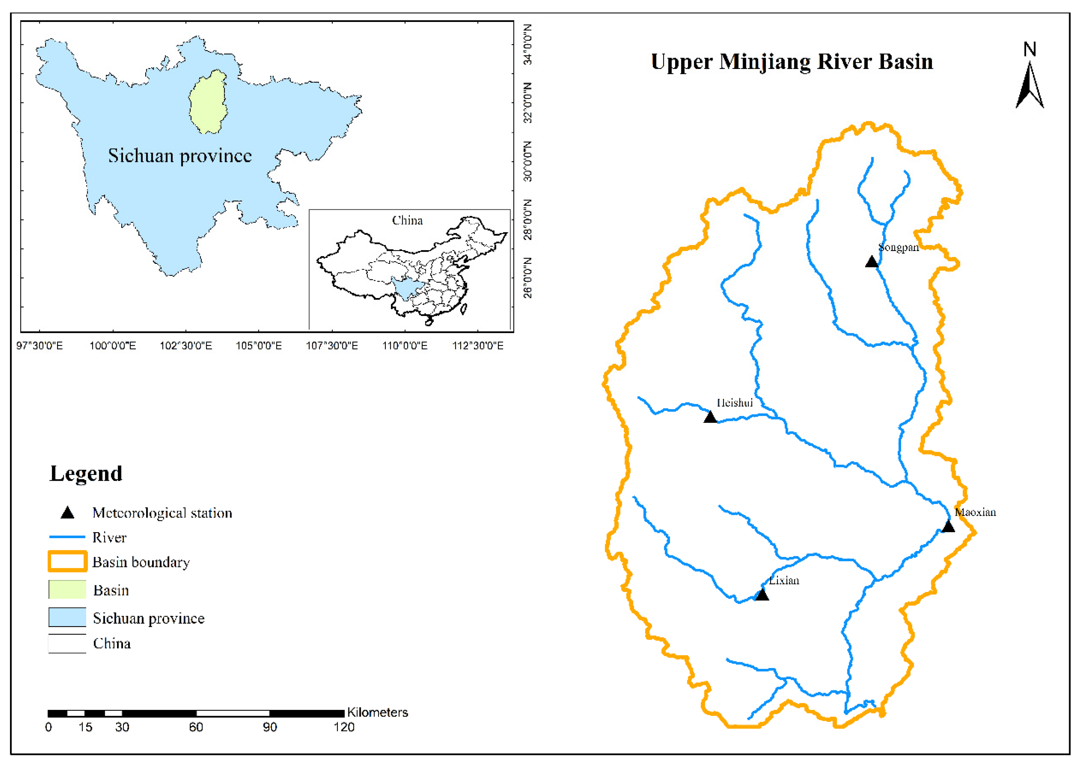
The study area in this paper is the upper Minjiang River basin (UMR). The UMR is located in Sichuan Province, China. There are many tributaries and dense river networks in the basin. It is the biggest tributary of the upper Yangtze River. The UMR is located on the southeastern edge of the Qinghai-Tibet Plateau, with high mountains and deep rivers in the area, its topography is low in the southeast and high in the northwest, which is a typical alpine valley landform [26,27]. However, due to the alternate control of the south tributary of the westerly wind, the warm Indian Ocean current, and the southeast Pacific monsoon, and under the influence of the complex and diverse geographical environment, the area has formed a unique arid valley climate feature: foehn winds in the area are strong, the atmosphere is dry all year round, and the dry and wet seasons are obvious. About 70% of annual precipitation is centralized in summer, with large annual evaporation, extreme drought in winter, and serious floods and drought disasters [25]. In addition, the UMR is located in the Longmenshan fault zone, the neotectonic movement is strong, which makes the entire mountain ecosystem fragile and changeable. In general, the UMR has a complex geographical environment and a fragile ecological environment [27]. Based on such a severe situation, the UMR was selected as the study area of this article.

The UMR basin includes all areas of Songpan, Lixian and Heishui, and parts of Wenchuan and Maoxian. There are a total of five meteorological stations. Due to the lack of precipitation data in some years in Wenchuan, this paper selects the precipitation data of other four stations as the data used in this study. Figure 1 shows that the selected four meteorological stations are evenly distributed in the UMR, which is reasonable.

The four meteorological stations in UMR were used to calculate the monthly precipitation data from the daily precipitation observation data from 1966 to 2016, and the monthly precipitation data were used for the calculation of SPI.

2.2. Method

2.2.1. Meteorological Drought Index Spi and Drought Characteristics

The drought index is an important variable used to assess the degree of drought and extract the drought characteristics (drought duration, drought severity, drought peak, etc.). Among them, SPI is one of the most widely used drought index s, which is recommended by the World Meteorological Organization for drought monitoring [28]. SPI was proposed by Mckee [8], its calculation is based on a multi-year monthly precipitation data series. The information of SPI response on different time scales is also different [29]. In this study, the SPIProgram downloaded from the website http://drought.unl.edu/Monitoring Tools/Downloadable SPIProgram.aspx (accessed on 15 January 2021) is only used to calculate the value of SPI on 1, 3 and 12 month time scales (SPI1, SPI3 and SPI12), the drought situation in the study area was analyzed by SPI3.

Table 1. Wet and drought period classification according to the SPI index.

Index Value	Class
SPI > −0.5	No drought
−0.5 ≥ SPI > −1.0	Mild drought
−1 ≥ SPI > −1.5	Moderately drought
−1.5 ≥ SPI > −2.0	Very drought
SPI ≤ −2.0	Extremely drought

lists the SPI climate classification provided by the national standards for meteorological drought levels issued by China. According to the classification in the table, this article sets the threshold for the beginning and end of the drought time as −0.5. In addition, according to the run theory proposed by Yevjevich [30], the drought characteristics based on SPI3 is extracted. This study uses drought duration, severity, and peak to analyze drought events. The three characteristics are defined as follows:

• Drought duration (D): The duration of SPI ≤ −0.5;
• Drought severity (S): The absolute value of the accumulated SPI value over the duration of the drought;
• Drought peak (P): The absolute value of the minimum SPI value during the duration of the drought.

Based on the preliminary identification of drought events, in order to avoid the impact of small drought events on the analysis of statistical characteristics of drought event samples, the following treatments are made for small drought events:

• Small drought events with drought duration of only 1 month and severity less than 1 were not included in the drought event sample;
• When the non-drought duration between two drought events is 1 unit period and the drought severity is less than −0.2, the two adjacent drought events will be merged into one drought event.

2.2.2. Mann-Kendall Test

The Mann-Kendall (MK) test is often used to test the changing trends of the meteorological and hydrological time series data. Its advantage is that the tested data series don’t have to follow a certain distribution [31]. The MK test null hypothesis H₀ is that the change trend of the data sequence X = {X₁, X₂, ……, Xn} is not significant. When the statistical parameter ∣Z∣ ≥ 1.96, the null hypothesis is rejected within the 95% confidence interval, that is, the trend of the data series is significant. When Z is positive, it means the trend is up, otherwise, it indicates a decline in the trend [32]. This paper uses the MK trend test method to check the significance of the downward or upward trend of the SPI sequences within the 95% confidence interval. The specific calculation process of the z value is as follows [33]:

$$S={\displaystyle \sum _{i=1}^{n-1}{\displaystyle \sum _{j=i+1}^{n}sign(x_j-x_i)}}$$

(1)

$$sign(x_j-x_i)=\{\begin{array}{c}1if(x_j-x_i)>0\\ 0if(x_j-x_i)=0\\ -1if(x_j-x_i)<0\end{array}$$

(2)

The formula for calculating the variance of S is:

$$\mathrm{var}(S)=\frac{n(n-1)(2n+5)-{\displaystyle \sum _{k-1}^m{t}_k(t_k-1)(2t_k+5)}}{18}$$

(3)

In Equation (3), n is the number of data, k is the number of repetitions, m is the number of unique numbers (the number of groups), and t_k is the number of repetitions for each repetition. When n > 10, the formula for calculating the statistical parameter Z is:

$$Z=\{\begin{array}{cc}\frac{S-1}{\sqrt{\mathrm{var}(S)}}& ifS>0\\ 0& ifS=0\\ \frac{S-1}{\sqrt{\mathrm{var}(S)}}& ifS>0\end{array}$$

(4)

2.2.3. Marginal Distribution

In order to establish a binary probability distribution between drought duration, severity and peak, we must first define the univariate distribution of these characteristics. Several alternative probability distributions functions are taken into consideration in this study, namely: Weibull (wbl), Normal, Log-normal (logn), Gamma (gam), Exponential (exp), Logistic (log), Log-logistic, General Extreme Value (gev), and Generalized Pareto (gpa) distribution. In this paper, the parameters of the marginal distribution are evaluated using the maximum likelihood estimation (MLE) method. Spearman (ρ) and Kendall (τ) are used to examine the correlation between different drought characteristics.

2.2.4. Chi-Square Test

In order to determine the best-fitting univariate marginal distribution of each characteristics, this study uses the chi-square test to estimate the best-fitting marginal distribution. The formula for calculating the chi-square value is as follows [5,34]:

$$x^2={\displaystyle \sum _{k=1}^n\frac{{(O_k-E_k)}^2}{E_k}}$$

(5)

Among them, n is the number of the disjoint group intervals; k is the serial number of the disjoint group intervals, O_k is the number of observations in the k-th disjoint group intervals; E_k is the expected number of observations in the k-th disjoint group intervals (according to the distribution being tested). The probability distribution function with the smallest Chi-Square value is chosen as the optimal distribution function.

2.2.5. Copula Function

The copula concept comes from Sklar’s theorem [35]. In the Copula function, the multivariate probability distribution and the univariate marginal distribution are connected by Sklar’s theorem. Then based on the joint cumulative probability distribution of the marginal distribution F1(x₁), F2(x₂), ……, Fn(x_n) (the x₁, x₂, ..., x_n are random variables), copula function can be defined [5]. Suppose that x and y are two random variables with joint distributions F_X,Y(x,y) and marginal distribution functions F_X(x) and F_Y(y), according to Sklar’s theorem [36], there is a Copula function C(x,y):

$$F_{X,Y}(x,y)=C(F_X(x),F_Y(y))$$

(6)

If F_X(x) and F_Y(y) are consecutive, this Copula is unique. On the contrary, if F_X(x), F_Y(y) and Copula function C(x,y) are given, the above formula defines the joint distribution function of F_X(x) and F_Y(y) [37,38,39].

Commonly used Copula functions are generally divided into five types, including Archimedean Copula, Metaelliptical Copula, Plackette Copula, mixed Copula, and empirical Copula. Since Archimedean Copula and Metaelliptical Copula functions are easy to construct and can capture dependent structures with several characteristics, they have become very attractive functions in bivariate hydrological frequency analysis [29,39]. In this paper, three commonly used Archimedean Copula (Clayton, Frank and Gumbol-Hougaard) and two commonly used Metaelliptical Copula (Gaussian and t Student Copula) were selected, and the inference function for margin (IFM) method [40] was used to estimate the parameters of copula functions, that is, first calculate the parameter values of the marginal distribution through the MLE method, and then use the obtained marginal distribution parameters to obtain the unknown parameters in the copula functions.

2.2.6. Function Evaluation

The fitting efficiency of the candidate Copula function is evaluated based on the Akaike Information Criterion (AIC). The smaller the value of AIC, the higher the fitting efficiency. The calculation method of AIC is as follows [6,41]:

$$\begin{array}{c}AIC=n\cdot \log (MSE)+2kandMSE=\left\{\frac{1}{n-k}{\displaystyle \sum _{i=1}^n{(X_C(i)-X_E(i))}^2}\right\}\\ \mathrm{or}AIC=-2\cdot \log (MLE)+2k\end{array}$$

(7)

Among them, k represents the number of fitting parameters, MSE represents the mean square error of the fitted copula function relative to the empirical copula, and X_C and X_E are the joint distribution functions based on the parameters and the empirical copula, respectively. MLE is the maximum likelihood of the copula function. Therefore, the copula with the smallest AIC value is the optimal copula.

2.2.7. Return Period

Shiau and Shen [42] proposed the return period theory of drought events. When the drought characteristic is greater than the preset value, the return period can be calculated from the expected value of the drought interval and the cumulative probability distribution corresponding to the characteristics. The calculation formula is:

$$T_D=\frac{E(L)}{1-F_D(D)}$$

(8)

$$T_S=\frac{E(L)}{1-F_S(S)}$$

(9)

$$T_P=\frac{E(L)}{1-F_P(P)}$$

(10)

In the formula, E(L) is the expected value of the drought interval. F_D(D), F_S(S), and F_P(P) are the cumulative probability distributions of drought duration, severity, and peak, respectively. T_D, T_S, and T_P are the D, S, and P recurrence period, respectively.

According to the nature of drought, univariate analysis may cause underestimation or overestimation of drought risk [37]. Drought characteristics are related random variables, so studying the joint regression period of these characteristic quantities is more helpful to the assessment of local drought risks and the management of water resources. This article will analyze the bivariate joint probability distribution. The bivariate joint return period between drought duration, drought severity, and drought peak is divided into two situations. Here, D and S are used as examples. The combination of other characteristics is the same: (1) The return period of D ≥ d and S ≥ s is expressed by T_DS; (2) The return period of D ≥ d or S ≥ s is expressed by T’_DS. The calculation method is as follows [6,42]:

$$T_{DS}=\frac{E(L)}{P(D\ge dandS\ge s)}=\frac{E(L)}{1-F_D(d)-F_S(S)+C(F_D(d),F_S(s))}$$

(11)

$$T^{’}{}_{DS}=\frac{E(L)}{P(D\ge dorS\ge s)}=\frac{E(L)}{1-C(F_D(d),F_S(s))}$$

(12)

3. Results and Discussion

3.1. Temporal and Spatial Trend of Drought Situation

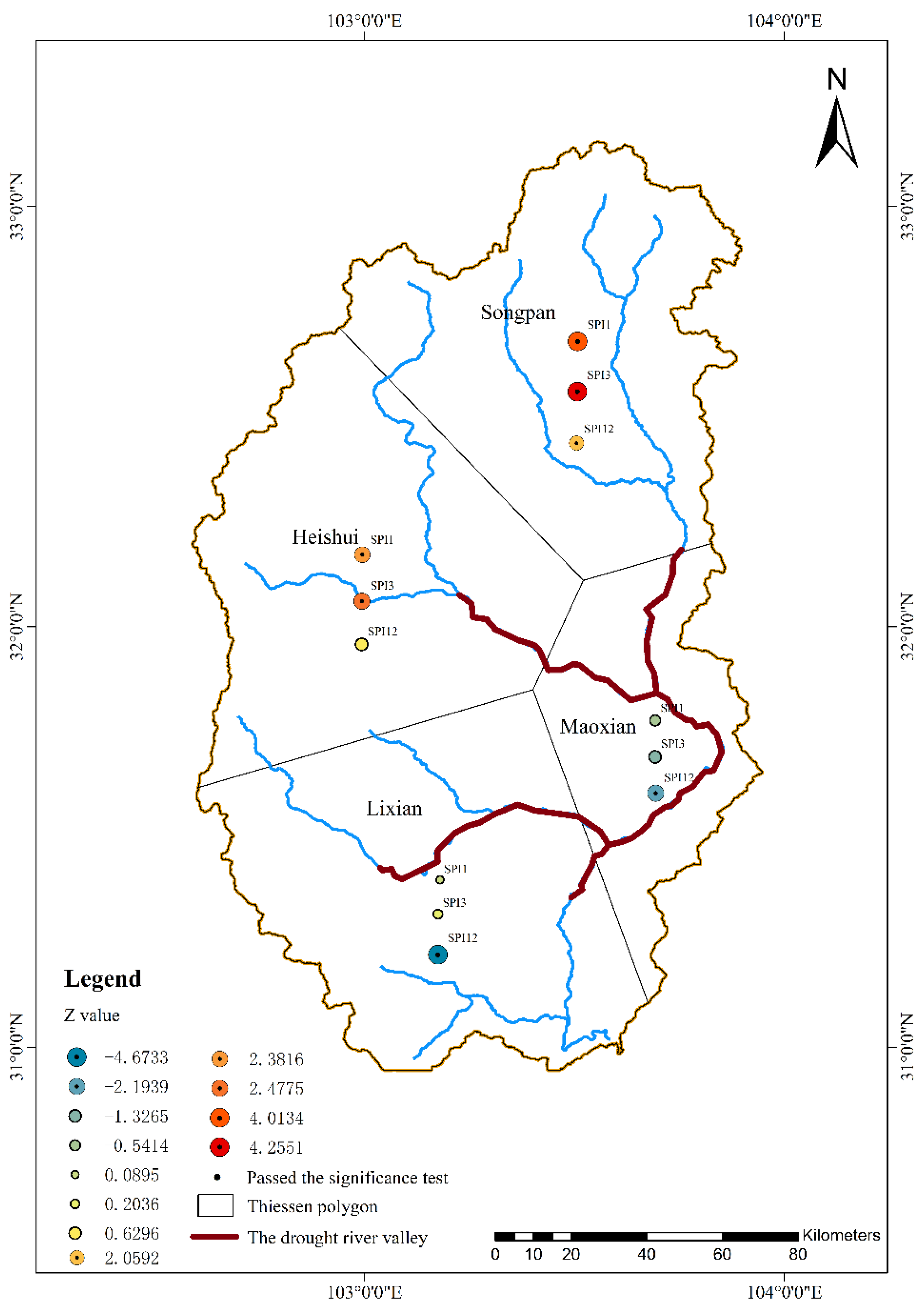
Based on the locations of 4 meteorological stations, the ArcGIS geographic information platform was used to generate Tyson polygons, and the study area was divided into four regions. In order to explore the changes in drought trends in various regions, this paper uses the MK trend test method to calculate the Kendall trend statistics of the SPI1, SPI3, and SPI12 at each meteorological station. The results are shown in

Table 2. Test results of change trend of drought index at different time scales.

Region	SPI	Z-Score	Slope	Change Trend
Songpan	SPI1	2.3816	0.0005	Significant upward trend
	SPI3	2.4775	0.0005	Significant upward trend
	SPI12	0.6296	0.0001	Unsignificant upward trend
Heishui	SPI1	4.0134	0.0009	Significant upward trend
	SPI3	4.2551	0.001	Significant upward trend
	SPI12	2.0592	0.0005	Significant upward trend
Maoxian	SPI1	0.0895	0	Unsignificant upward trend
	SPI3	0.2036	0	Unsignificant upward trend
	SPI12	−4.6733	−0.0011	Significant downward trend
Lixian	SPI1	−0.5414	−0.0001	Unsignificant downward trend
	SPI3	−1.3265	−0.0003	Unsignificant downward trend
	SPI12	−2.1939	−0.0005	Significant downward trend

and Figure 2. According to the statistical distribution shown in Figure 2, the UMR can be divided into two categories, Songpan and Heishui are classified as Class I region, Maoxian and Lixian are classified as Class II region. The change trend of drought index in all time scales of Class I was significantly increasing except SPI12 in the Heishui region, which was not significantly increasing. The rising trend of SPI on the 1-month and 3-month (not cross-seasonal) timescales was more significant than the SPI on the 12-month timescales. The SPI sequence of Class II region showed a general downward trend, indicating that drought events were more likely to occur in Class II regions than before. Table 2 shows that on the time scale of 1 month and 3 months, although the drought index sequence of Maoxian region shows an upward trend, its trend rate is 0 (in fact, it is a positive number very close to 0). It can be seen that the upward trend is extremely insignificant. On a 12-month (cross-season) scale, the SPI series of Maoxian and Lixian have a significant downward trend. The statistical results show the historical dry-wet evolution phenomenon of humidification in short-term and drought in long-term in the UMR.

The distribution of the dry valleys in the UMR is showed in Figure 2. It can be seen that the dry valleys are distributed in all the mainstreams of the UMR in Maoxian region, and part of the mainstreams of the UMR in Heishui and Lixian regions. The length of the dry valley in Maoxian region is the longest, followed by Lixian region. Combining the calculation results of the SPI change trend, it can be seen that, relatively speaking, the Maoxian and Lixian regions where the dry valleys are more widely distributed are more likely to become drier, that is, there is a greater risk of drought.

3.2. Meteorological Drought Assessment

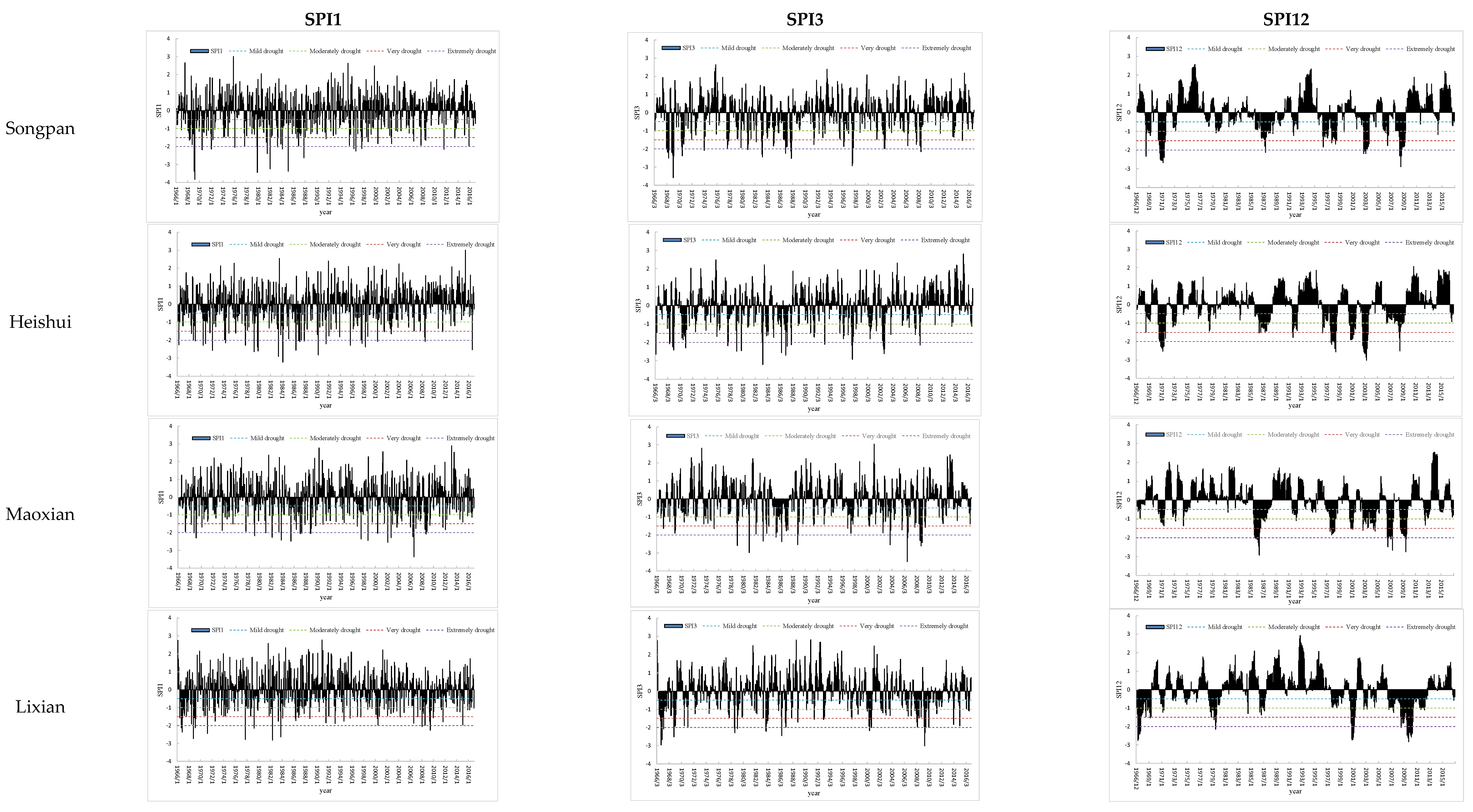
SPI of different time scales reflects the different cumulative effect of drought. Figure 3 shows the SPI1, SPI3, and SPI12 sequences of the four regions. Comparing the three sequences of SPI1, SPI3, and SPI12, it can be seen that the SPI with a shorter time scale (SPI1 and SPI3) is more discrete, drought events occur more frequently, which means that the SPI with a short time scale is more capable of responding to small drought events. The long-term SPI(SPI12) treats several consecutive minor drought events as one drought event, so the long-term SPI can better reflect the long-term trend of drought, and relatively speaking, drought events last longer.

It can be found from the SPI sequences (Figure 3): in the Songpan region, from 1966 to 1972, from 1978 to 1991, and from 1996 to 2008, the SPI values were mostly negative, and the SPI values in other periods were mostly positive. This means that most of the drought events occurred in the period from 1966 to 1972, from 1978 to 1991, and from 1996 to 2008. In Heishui region, SPI was mostly negative from 1966 to 1972, from 1986 to 1987, and from 1996 to 2008, and SPI was mostly positive in other periods; in the Maoxian region, the frequency of positive and negative SPI was similar from 1966 to 1975, and the SPI was mostly negative from 1985 to 1988 and from 1991 to 2010, it can be seen that the drought lasted for a long time in the Maoxian region; in the Lixian region, SPI was mostly negative from 1966 to 1969, 1978–1980, and 1997–2012, and mostly positive in other periods. Meanwhile, Figure 3 shows that drought events occurred more frequently in Lixian during 1997–2012, and the drought was more serious.

It can be seen from the comparison of SPI sequences of different time scales, compared with SPI1, SPI3 can integrate some small drought events, which is suitable for seasonal drought and can better reflect agricultural drought scenarios. Therefore, this study is mainly based on SPI3 for drought assessment.

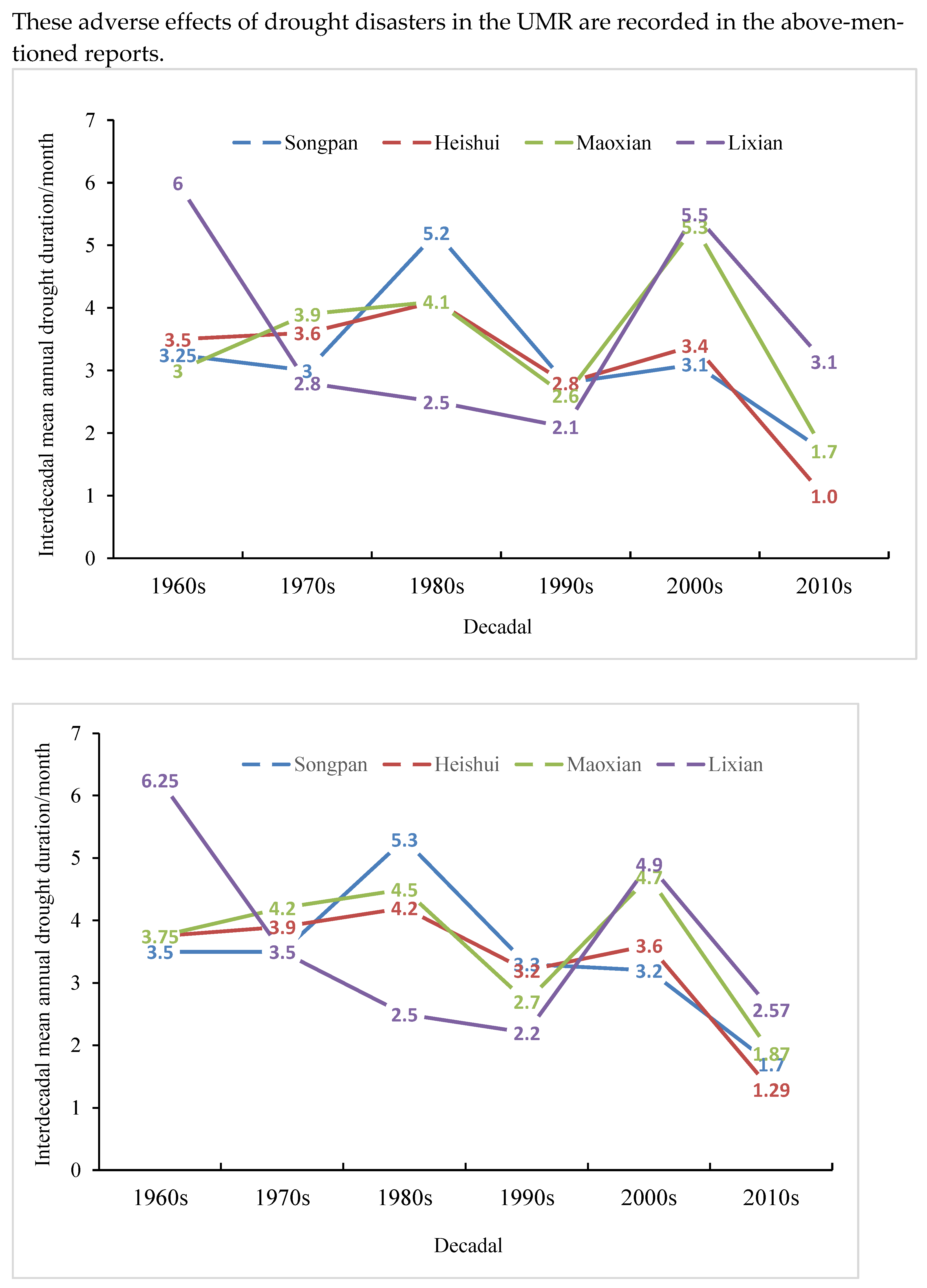
According to the calculated SPI value, the drought characters of D, S, and P can be extracted to evaluate the drought. Based on the SPI3, the drought duration in Songpan, Heishui, Maoxian, and Lixian regions from 1965 to 2016 were 166, 160, 183, and 175 months, respectively. The drought duration of each region on the interdecadal scale (1960s (1966~1969), 1970s (1970~1979), 1980s (1980~1989), 1990s (1990~1999), 2000s (2000~2009), and 2010s (2010~2016)) was accounted and analyzed, the results were shown in Figure 4. Figure 4 shows that the drought duration of Songpan and Heishui in the 1980s and 2000s was longer than that of other decades. Maoxian region in the 1980s and 2000s had a longer drought duration, while Lixian region in the 1960s and 2000s had a longer drought duration. The drought duration of the four regions in 2010s was relatively short. Overall, the drought duration was relatively long in the 1980s and 2000s and was the shortest in the 2010s.

All historical drought events in four regions from 1966 to 2016 were analyzed as follows. According to monthly statistics, historical drought events in Songpan mostly occurred in March; historical drought events in Heishui mostly started in January, June and December; and historical drought events in Maoxian mostly started in March June and October, historical drought events in Lixian mostly started in January, February, and April. According to seasonal statistics, drought events mostly occurred in spring and winter in the Songpan region, the proportion are 29.17% and 29.17%, respectively. In the Heishui region, the proportion of drought events that occurred in winter was 36.17%. The proportion of drought events in spring and summer was 27.66% and 29.79%, respectively, in the Maoxian region. In the Lixian region, the proportion of drought events that occurred in spring and winter was 24.49% and 32.65%, respectively.

Table 3. Statistics of severe drought events in various regions from 1966 to 2016.

Region	The Beginning and End of the Drought	Severity of Drought (S)
Songpan	February to July 1968	S = 12.64
	December 1968 to April 1969	S = 11.46
	June to December 1970	S = 12.07
	September 1986 to April 1987	S = 12.92
Heishui	May 1970 to March 1971	S = 16.08
	September 1986 to May 1987	S = 11.99
	July to November 1997	S = 9.84
	June to December 2002	S = 13.5
Maoxian	June 1985 to June 1986	S = 16.48
	January 1997 to January 1998	S = 12.79
	July 2006 to February 2007	S = 11.4
	July 2008 to February 2009	S = 14.02
Lixian	July 1966 to June 1967	S = 19.13
	May to December 2000	S = 12.22
	January to September 2006	S = 14.65
	April to October 2009	S = 11.52

lists some of the more serious drought events. It shows that the drought duration in Maoxian and Lixian is not only longer than that in the other two regions, but the severity of major historical drought events is also stronger than that in other regions, indicating that the drought risk in Maoxian and Lixian is relatively high.

According to news reports, most of the drought disasters in Sichuan in the past 20 years occurred in the 2000s, which confirms the reliability of our above analysis. On 10 April 2005, Sichuan Online-West China Metropolis Daily reported the phenomenon of “Minjiang Dehydration”. The reporters found in Nanxin Town, Maoxian that the UMR had dried up and the sand was cracked, like a Gobi (http://news.sina.com.cn/o/2005-04-10/07385606826s.shtml, the accessed date is 7 July 2021). On 20 August 2006, Sichuan Online-Huaxi Metropolis Daily reported the phenomenon of “Minjiang River Drying”. The snow cover of the five counties in the UMR in 2006 was lower than usual and showed a trend of decreasing year by year. The riverbed in Mianchi Township of Wenchuan dried up and cracked (http://news.sina.com.cn/c/2006-08-20/07389796123s.shtml, the accessed date is 8 July 2021). On 4 April 2007, Sichuan Online-Huaxi Metropolis Daily reported that Sichuan is facing a severe drought in spring and summer, and 5.9 million people have difficulty drinking water (http://news.sohu.com/20070404/n249186525.shtml, the accessed date is 8 July 2021). Sichuan News Net-Chengdu Business Daily reported on 27 February 2010 that since 2010, the western Sichuan Plateau has been experiencing high temperatures and low precipitation, there has been a phenomenon of droughts in autumn and winter, and the mountain snow cover was nearly 50 percent less than last year, or even at the same time for many years in February 2010.

These drought disasters have brought severe impacts on the local area in many ways:

• Impact on humans: it has caused difficulties in drinking water for humans and animals; the dry-flow area of the Minjiang River cuts off the sources of income for residents in nearby areas who feed on and wash cars along the way; frequent “dehydration” in several sections of the Minjiang River directly affects humans when it comes to urban and rural life and industrial and agricultural production that rely on the Minjiang River for water supply;
• Impact on agriculture: the continuous drought has caused the crops grown by local residents to turn yellow and reduce production, the supply of agricultural products is insufficient, and the price rises;
• Impact on wild and rare animals: The construction of water conservancy projects in the UMR has changed the natural properties of the runoff and has caused a serious impact on the aquatic animals and plants of the Minjiang River. The fish species in the UMR have dropped from 40 species in the 1950s to 16 species today;
• Impact on the environment: continuous drought has reduced the capacity of the water environment, which has aggravated the water pollution of the Minjiang River and the deterioration of the water environment. These adverse effects of drought disasters in the UMR are recorded in the above-mentioned reports.

3.3. Marginal Distribution

To explore the joint distribution of bivariate, we must first determine the marginal distribution of univariate. Calculate the value of SPI3 in each region, using Weibull (wbl), Normal, Log-normal (logn), Gamma (gam), Exponential (exp), Logistic (log), Log-logistic, General Extreme Value (gev), and Generalized Pareto (gpa) distribution functions fit the marginal distribution of D, S, and P, respectively. The chi-square goodness of fit test was used to select the optimal marginal distribution of drought duration, severity, and peak in each region under the condition of significance level α = 0.05. The optimal marginal distribution and the corresponding parameters estimated by maximum likelihood were shown in

Table 4. Marginal distribution of drought characteristics in each region.

Region	Drought Duration	Parameter	Drought Severity	Parameter	Drought Peak	Parameter
Songpan	exp	μ = 3.4583	logn	μ = 1.2298	logn	μ = 0.3538
				σ = 0.7807		σ = 0.4053
Heishui	logn	μ = 1.0577	log-logistic	μ = 1.2213	logn	μ = 0.4216
		σ = 0.5916		σ = 0.3970		σ = 0.3603
Maoxian	log-logistic	μ = 1.1237	log-logistic	μ = 1.1868	log	μ = 1.4769
		σ = 0.3614		σ = 0.3955		σ = 0.3550
Lixian	log-logistic	μ = 1.1060	log-logistic	μ = 1.1455	logn	μ = 0.3749
		σ = 0.3238		σ = 0.3813		σ = 0.3595

. Table 4 illustrates that the Exponential, Log-normal, and Log-logistic distribution were selected as the best marginal distribution of the drought duration in the four regions. Log-normal and Log-logistic were chosen as the optimal marginal distributions of the drought severity characteristics in the four regions, the best marginal distributions of drought peak were Exponential, Log-normal, and Logistic. Therefore, for the characteristic of drought duration and drought severity, it is a good choice to use Log-Logistic distribution as their marginal distribution. Log-normal distribution also has good applicability for drought peak. According to the parameter values of the best marginal distribution provided in Table 4, the value of each characteristic quantity corresponding to a specific cumulative distribution probability can be easily calculated according to needs.

In order to measure the correlation between the three characteristics of drought duration, drought severity, and drought peak, the Spearman (ρ) and Kendall (τ) correlation parameters between different drought characteristics were calculated. The closer the correlation coefficient is to 1, the stronger the correlation.

Table 5. Correlation coefficients among drought characteristics.

Region	D-S		D-P		S-P
	Spearman (ρ)	Kendall (τ)	Spearman (ρ)	Kendall (τ)	Spearman (ρ)	Kendall (τ)
Songpan	0.851 **	0.757 **	0.640 **	0.458 **	0.807 **	0.614 **
Heishui	0.886 **	0.757 **	0.424 **	0.318 **	0.740 **	0.556 **
Maoxian	0.857 **	0.727 **	0.342 *	0.247 *	0.721 **	0.530 **
Lixian	0.851 **	0.732 **	0.590 **	0.463 **	0.864 **	0.691 **

** indicates that the correlation coefficient has passed the significance test of α = 0.01. * indicates that the correlation coefficient has passed the significance test of α = 0.05.

shows the calculation results. The calculation results indicate that the Spearman correlation coefficients of D and S are all higher than 0.851, reaching the maximum in Heishui area (0.886), and the Kendall correlation coefficients are all higher than 0.727, and reaching the maximum value (0.757) in Songpan and Heishui regions; the Spearman correlation coefficient of S and P are all higher than 0.721, reaching the maximum in Lixian region (0.864), Kendall correlation coefficients are all higher than 0.530, and also reaching the maximum in Lixian region (0.691), which shows that there is a significant correlation between the two pairs of characteristics. Although the correlation coefficient value of D and P are smaller than the other two pairs of characteristic combinations, the correlation coefficients of Songpan, Heishui, and Lixian regions have passed the significance test of α = 0.01, and the correlation coefficients of Maoxian have passed the significance test of α = 0.05, which shows that there is a significant correlation between each characteristic. Since the positive correlation between the drought characteristics and the good fitting effect of each characteristic through different distribution functions, the copula function can be used to simulate the joint probability distribution between the drought characteristics.

3.4. Joint Distribution of Drought Characteristics

This study used five common copula functions, Clayton, Frank, Gumbol-Hougaard, Gaussian, and t Student copulas, to set up the joint distribution of the drought characteristics based on SPI3, and the AIC method is used to evaluate the best copula function.

The AIC value in

Table 6. AIC evaluation value of each copula function.

Region	D-S		D-P		S-P
	Copula	AIC Value	Copula	AIC Value	Copula	AIC Value
Songpan	t Student	−28.2717	t Student	−10.7198	t Student	−46.2465
	Gaussian	−27.6555	Gaussian	−13.1397	Gaussian	−48.1792
	Clayton	−15.7287	Clayton	−3.3449	Clayton	−32.6926
	Frank	−31.5535	Frank	−15.8140	Frank	−46.4643
	Gumbol	98.6545	Gumbol	−14.7983	Gumbol	−46.8826
Heishui	t Student	−69.6858	t Student	−3.2975	t Student	−30.5845
	Gaussian	−71.6859	Gaussian	−5.2975	Gaussian	−32.5845
	Clayton	−47.6935	Clayton	−1.4329	Clayton	−24.5563
	Frank	−63.0136	Frank	−4.8052	Frank	−30.1821
	Gumbol	90.2540	Gumbol	−4.9524	Gumbol	−29.6669
Maoxian	t Student	−70.0885	t Student	−4.2993	t Student	−32.0909
	Gaussian	−72.0882	Gaussian	−6.2992	Gaussian	−34.0903
	Clayton	−49.3726	Clayton	−1.2425	Clayton	−30.0014
	Frank	−61.1346	Frank	−5.1332	Frank	−33.1516
	Gumbol	73.1808	Gumbol	−5.4247	Gumbol	−26.4213
Lixian	t Student	−76.8539	t Student	−15.7463	t Student	−53.7382
	Gaussian	−78.3507	Gaussian	−17.7463	Gaussian	−55.7379
	Clayton	−56.7514	Clayton	−4.4238	Clayton	−27.8824
	Frank	−66.0320	Frank	−16.5257	Frank	−54.2777
	Gumbol	82.8494	Gumbol	−22.8013	Gumbol	−57.3134

indicates the appropriateness of t Student, Gaussian, Clayton, and Frank to establish the joint distribution of D-S. Gumbol-Hougaard is not applicable to establish the joint probability distribution of D-S at all regions. The five copula functions of Clayton, Frank, Gumbol-Hougaard, Gaussian, and t Student copulas are all suitable for describing the joint probability distribution of S-P, as well as D-P. The copula function with the smallest AIC value is selected as the optimal copula function of the bivariate joint probability distribution of each region. The best copula function and the corresponding parameters are shown in

Table 7. The optimal copula function of the bivariate joint distribution of each region.

Region	D-S		D-P		S-P
	Copula	Parameter	Copula	Parameter	Copula	Parameter
Songpan	Frank	6.9027	Frank	4.7848	Gaussian	0.8053
Heishui	Gaussian	0.8898	Gaussian	0.3792	Gaussian	0.7219
Maoxian	Gaussian	0.8907	Gaussian	0.4016	Gaussian	0.7320
Lixian	Gaussian	0.8987	Gaussian	0.5760	Gaussian	0.8324

. Table 7 indicates that Gaussian and Frank copula functions are the best copula functions of D-S, as well as D-P. The best copula function of S-P is Gaussian copula function. It can be found from the optimal copula functions that for the entire UMR, the Gaussian Copula function is a good choice for simulating the joint distribution of D-S, D-P, and S-P.

3.5. Frequency Analysis of Drought Characteristics in Univariate and Bivariate

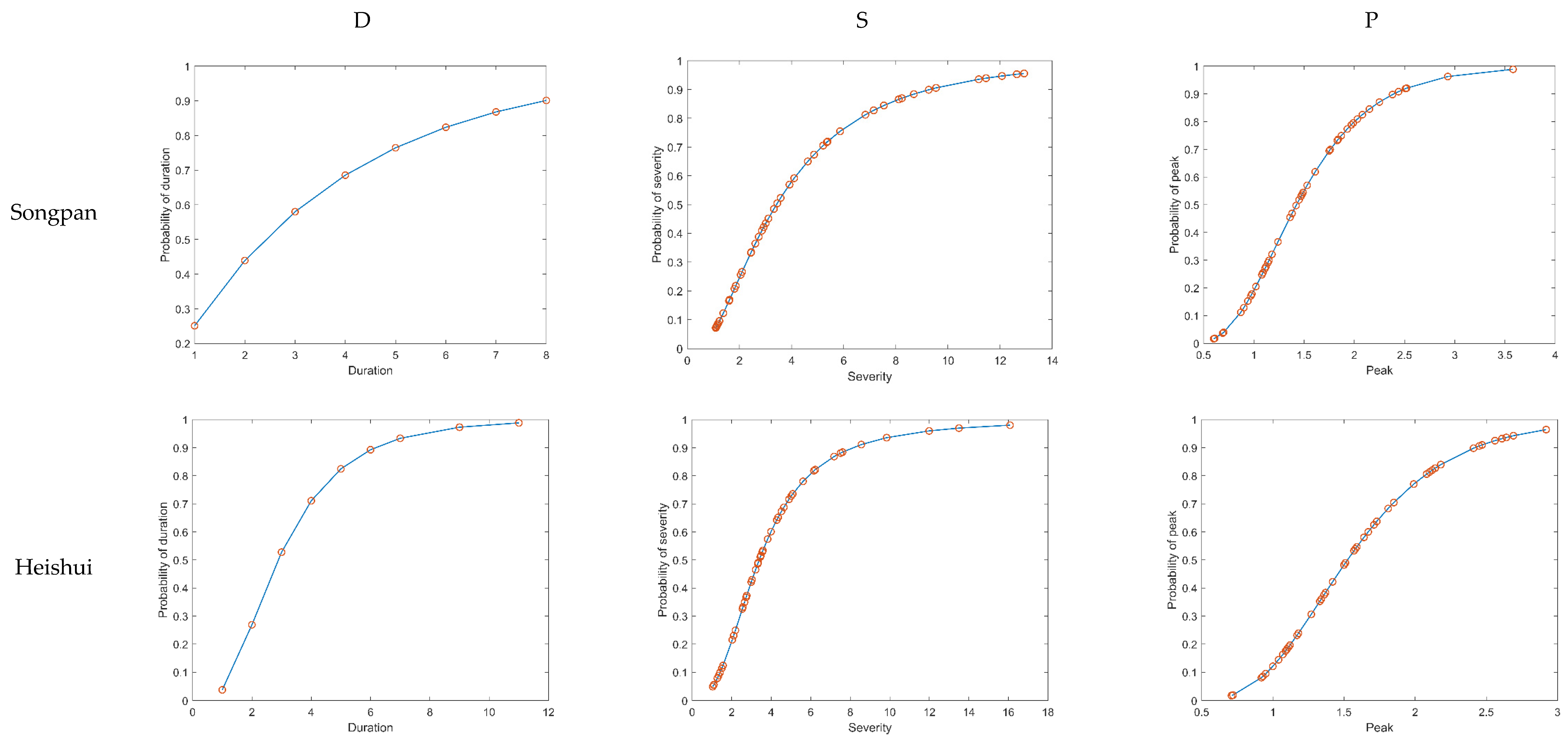
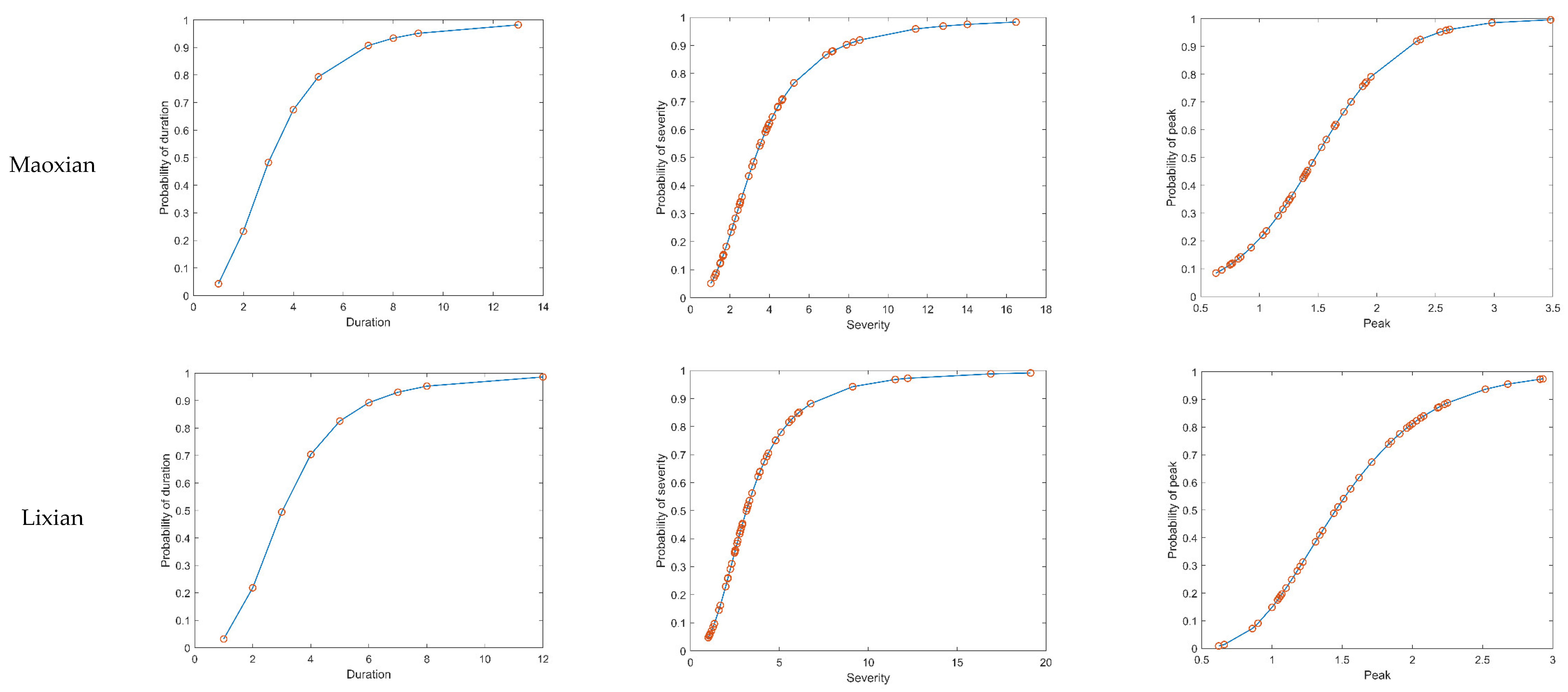
According to the best marginal distribution of each characteristic selected in Section 3.3, this paper gives the univariate cumulative probability distribution diagram of each characteristic through calculation. As shown in Figure 5, the cumulative probability value corresponding to the specific value of the characteristic can be read. For example, when the cumulative probability P(X ≤ x) in Maoxian area is 0.8, the corresponding drought duration (D) is 5.01 months, the drought severity (S) is 5.78, and the drought peak (P) is 1.95.

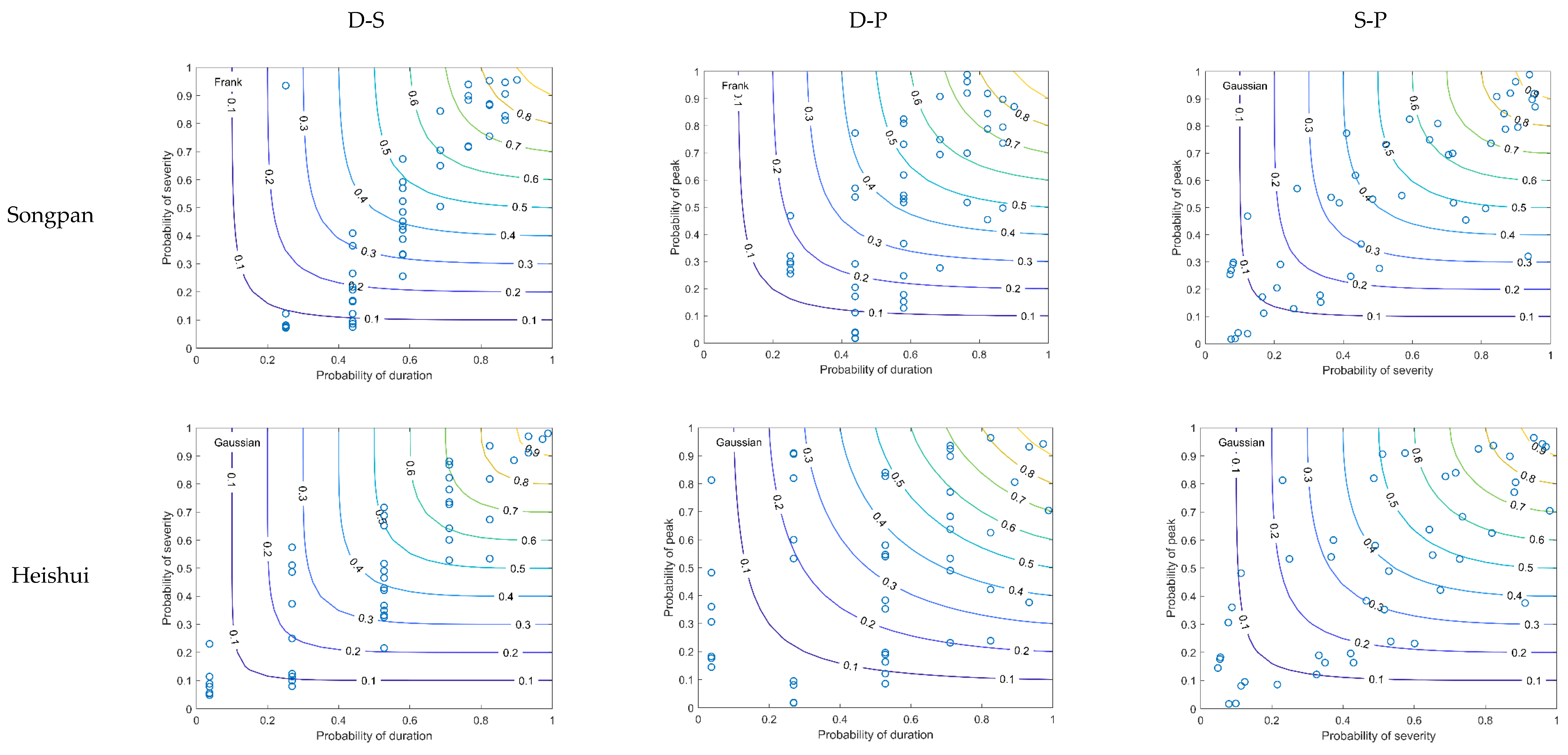
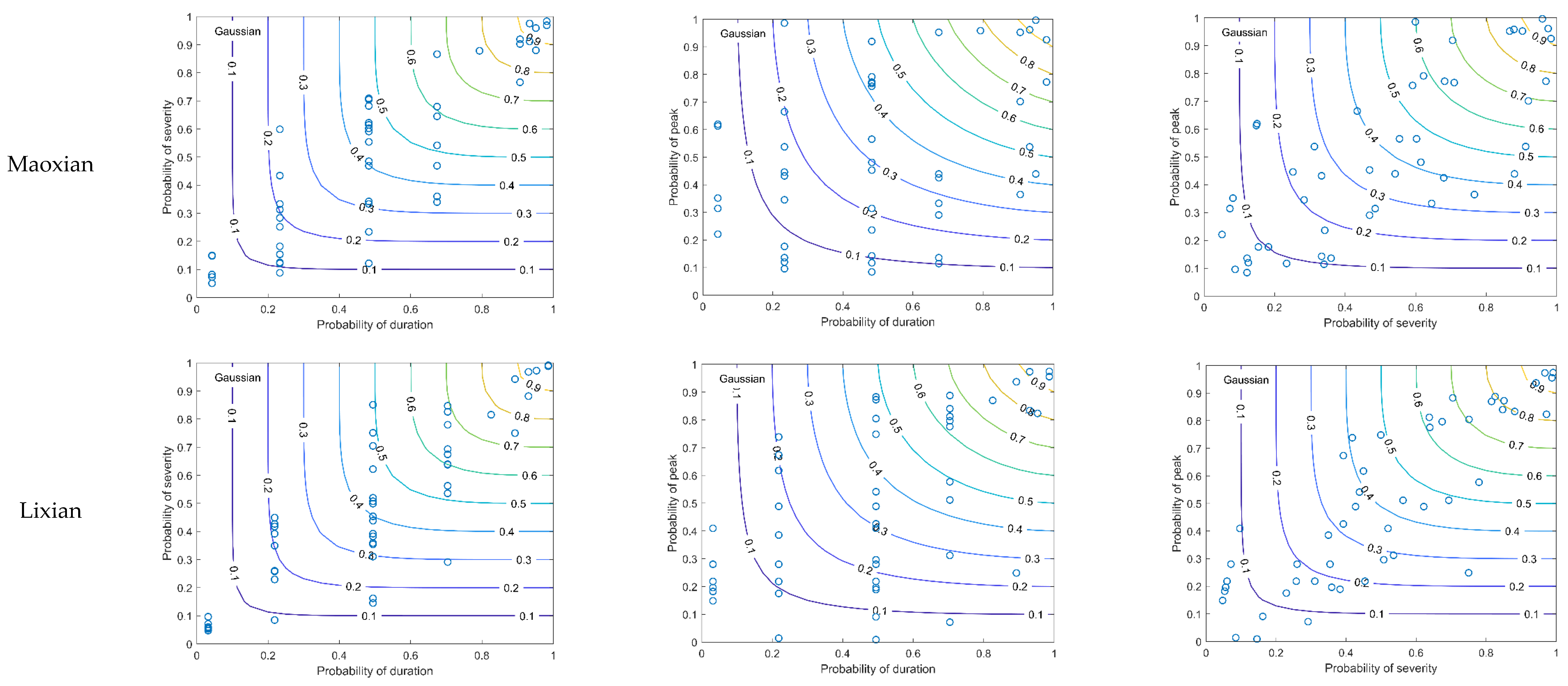
According to the optimal copula function of the bivariate joint distribution of drought characteristics selected in Chapter 3.4, the bivariate joint probability distribution based on SPI3 (including P(D ≤ d, S ≤ s), P(D ≤ d, P ≤ p) and P(S ≤ s, P ≤ p)), the joint probability distribution of the bivariate drought characteristics can be read from Figure 6. For example, when the cumulative probability of D, S and P in Maoxian area is 0.8, the bivariate joint probability P(D ≤ 5.01, S ≤ 5.78) is 0.7562, and P(D ≤ 5.01, P ≤ 1.95) is 0.6764, and P(S ≤ 5.78, P ≤ 1.95) value is 0.7177. These results will help quantify the frequency of drought events of different degrees.

3.6. Return Period Analysis

Return period analysis is an important part of drought assessment. For the determination of the drought return period, the expected value of the drought interval must first be determined. According to the analysis of drought characteristic variables, the expected drought interval E(L) for the four regions of Songpan, Heishui, Maoxian, and Lixian are 12.71, 12.97, 12.98, and 12.27 months, namely 1.0590, 1.0807, 1.0816, and 1.0226 years, which are similar to 1 year. The meteorological drought interval in southwest China is reported to be mainly affected by the superposition of monsoon and drought disturbances. The drought disturbances are mainly related to the ENSO circulation, which is closely related to the interannual planetary westerly disturbance and the interannual SST disturbance at the equator [43].

First the univariate return period (T) levels are taken to be 2, 5, 10, 20, and 50a; the corresponding values of D, S, and P are calculated, respectively, and the corresponding two-dimensional Copula function values are calculated by the optimal Copula functions of different characteristic variables. According to Equations (11) and (12), the corresponding bivariate joint return periods at a given univariate return period level are calculated. The computed values are showed in

Table 8. Return periods of joint distribution of drought characteristics.

Region	T/(a)	D/(m)	S	P	D-S		D-P		S-P
					T/a	T’/a	T/a	T’/a	T/a	T’/a
Songpan	2	2.2395	3.2300	1.3825	2.4418	1.6936	2.6271	1.6146	2.467	1.6804
	5	4.4017	6.4254	1.9702	8.1839	3.5996	9.7694	3.3598	7.6023	3.7249
	10	6.7901	9.0771	2.3645	23.3260	6.3642	29.1736	6.0342	17.4178	7.0132
	20	8.7848	12.0887	2.7801	74.0559	11.5611	98.0556	11.1356	39.5149	13.3881
	50	12.4807	15.7218	3.3386	−398.1203	26.2751	540.3061	26.2129	115.6114	31.8976
Heishui	2	2.7375	3.1812	1.4701	2.3226	1.7561	3.0589	1.4857	2.5768	1.6342
	5	4.6431	5.6618	2.0244	7.0912	3.9849	14.4479	3.0983	9.0435	3.5538
	10	5.9894	7.8725	2.3855	14.7355	7.5679	37.7339	5.7637	20.1849	6.6464
	20	7.6368	10.7294	2.7262	32.0018	14.5451	108.3952	11.0163	47.6709	12.6546
	50	9.7106	15.5482	3.1969	88.3791	34.8613	427.4921	26.5528	147.4754	30.1031
Maoxian	2	2.9060	3.0720	1.4188	2.3205	1.7573	3.0238	1.4941	2.5618	1.6403
	5	4.9202	5.5221	1.9341	6.6997	3.9882	12.5709	3.1206	8.3238	3.5732
	10	6.7365	7.5708	2.2566	14.6717	7.5849	35.9097	5.8088	19.8023	6.6889
	20	8.6969	10.46945	2.4997	31.9433	14.5572	101.4634	11.0933	46.5004	12.7397
	50	12.5496	14.9461	2.8703	88.1931	34.8903	391.3169	26.7062	142.9931	30.2969
Lixian	2	2.9797	3.0913	1.4401	2.3289	1.7525	2.8477	1.5412	2.4470	1.6911
	5	4.7525	5.2891	1.9535	6.6645	4.0008	10.3043	3.3008	7.3706	3.7832
	10	6.1348	7.3876	2.3063	14.5214	7.6257	26.5472	6.1602	16.6493	7.1461
	20	7.8213	9.7371	2.6239	31.4066	14.6714	67.9017	11.7271	37.2396	13.6711
	50	11.2152	14.3690	3.0104	86.6317	35.1409	232.1980	28.0164	106.4765	32.6709

.

Table 8 illustrates that the univariate return period is between the joint return period T (‘and’ event) and T’ (‘or’ event). The bivariate joint return period T is always bigger than T’, because the calculation of the return period of the ‘and’ event is more restrictive than that of the ‘or’ event. Taking the Maoxian region as an example, the 50-year return periods of univariate of D and S are both between the T_DS = 88.1931a and the T’_DS = 34.8903a. In addition, under the same univariate return period level, the duration of drought in Maoxian was greater than that of the other three regions, and the severity and peak of drought in Songpan were greater than those of the other three regions, which indicates that the drought duration of Maoxian lasted longer than other three regions, and the severity and peak of the drought in the Songpan is more severe than other regions. Since the optimal marginal distribution function and optimal copula function have been obtained above, and the corresponding parameters have been calculated, in addition to the return periods corresponding to the drought events of different degrees that have been calculated in Table 8, the return period corresponding to the value of a particular drought duration, drought severity, or drought peak can also be determined according to need.

4. Conclusions and Suggestions

4.1. Conclusions

Drought assessment is critical to water resources planning and management. This article aims to comprehensively analyze the meteorological drought in the UMR.

In this paper, the change trends of SPI in different time scales in four regions were analyzed. The results show that the SPI sequence on a short time scale is more discrete and more able to reflect small drought events. The long-term SPI can better reflect the long-term trend of drought. The UMR showed the historical dry-wet evolution of humidification in short-term and drought in long-term. By analyzing the trend of SPI at various time scales, it is found that Maoxian and Lixian regions where the dry valleys are more widely distributed are more likely to become more arid.

Based on SPI3, the duration, severity, and peak of meteorological drought were estimated, and the drought events in each region were calculated. The results showed that the drought lasted the longest in Maoxian from 1966 to 2016, which was 183 months, the droughts in Songpan, Heishui, and Lixian lasted 166, 160, and 175 months, respectively. According to the decadal statistics of the drought duration in each region, the results show that the drought duration in the study area was relatively long in the 1980s and 2000s, and the drought duration was the shortest in 2010s. Drought events in the study area mostly started in winter and spring. Compared with the statistics of notable drought events in different regions, Maoxian not only has a longer drought duration, but also has a higher severity of historical drought events. Lixian has the highest severity of drought events in history.

According to the results of the chi-square test, this study determines the optimal marginal distribution of drought characteristics from Weibull (wbl), Normal, Log-normal (logn), Gamma (gam), Exponential (exp), Logistic (log), Log-logistic, General Extreme Value (gev), and Generalized Pareto (gpa) distribution functions. For drought duration, it is a good choice to use Log-logistic distribution as its marginal distribution. Log-normal distribution also has good applicability for drought peaks. The drought severity in different regions has different optimal marginal distributions, including Exponential, Log-normal, Logistic, and Log-logistic distributions.

Due to the dependence of the drought characteristics, this study uses Clayton, Frank, Gumbol-Hougaard, Gaussian and t Student five copula functions to fit the bivariate joint distribution to present a more realistic joint distribution result. According to the AIC value, the joint distribution of drought characteristics that is most suitable to describe each region is determined. The results show that due to differences in the correlation between drought characteristics in different regions, the applicable copula functions may also be different. For example, the optimal copula functions for D-S and D-P in different regions include Gaussian and Frank copula functions. As far as the entire study area is concerned, the Gaussian copula function is a good choice for the simulation of the joint probability distribution of the D-S, D-P and S-P.

In addition, based on the optimal marginal distribution and the optimal copula function, this paper calculates the univariate return period and the bivariate joint return period of drought characteristics to reflect the frequency of drought events of different degrees.

In general, Maoxian and Lixian have a higher risk of drought than Songpan and Heishui. According to the drought indices at different scales, almost all the SPI sequences at different scales in Songpan and Heishui showed an obvious increasing trend, while the SPI12 in Maoxian and Lixian showed an obvious trend of becoming drier. Maoxian has the longest drought duration among the four historical drought events. From the perspective of drought severity, the historical drought events in Lixian were more serious than those in the other three regions. However, this does not mean that the drought disaster in Songpan and Heishui is not serious, because except for Maoxian, the drought lasted for 183 months, the historical drought duration in the other three regions is more than 160 months, and serious drought events have occurred in all regions.

In short, the results of this paper can supply effective information for the study area to assess drought risk, so as to optimize the allocation of water resources and reduce the impact of drought on the UMR in the future.

4.2. Suggestions

Due to the frequent occurrence of drought disasters in the UMR, this article puts forward some suggestions for drought disaster management.

First of all, a good ecological environment is a strong barrier against drought disasters. Aiming at the fragile ecological environment in the UMR, new drought-resistant tree species can be cultivated, and various types of plants such as arbor, shrubs, grass, and cane can be planted to build a multi-level structure of the forest system to strengthen ecological barriers. Secondly, local residents can choose to plant crops with strong drought resistance to avoid the residents’ diet from being greatly affected when drought disasters occur. Based on the concept of water conservation, relevant departments of the Sichuan government can re-allocate the limited water resource input in terms of urban and rural life, industrial and agricultural production, encourage and promote residents and factories in Sichuan to take concrete water-saving measures, and improve people’s water-saving awareness.

References

- Ali, Z.; Almanjahie, I.M.; Hussain, I.; Ismail, M.; Faisal, M. A novel generalized combinative procedure for Multi-Scalar standardized drought Indices-The long average weighted joint aggregative criterion. Tellus Ser. A Dyn. Meteorol. Oceanogr. 2020, 72, 1–23. [Google Scholar] [CrossRef] [Green Version]
- Dai, A.; Trenberth, K.E.; Qian, T.T. A global dataset of Palmer Drought Severity Index for 1870–2002: Relationship with soil moisture and effects of surface warming. J. Hydrometeorol. 2004, 5, 1117–1130. [Google Scholar] [CrossRef]
- Yang, J.; Chang, J.; Wang, Y.; Li, Y.; Hu, H.; Chen, Y.; Huang, Q.; Yao, J. Comprehensive drought characteristics analysis based on a nonlinear multivariate drought index. J. Hydrol. 2018, 557, 651–667. [Google Scholar] [CrossRef]
- Duan, K.; Mei, Y. Comparison of Meteorological, Hydrological and Agricultural Drought Responses to Climate Change and Uncertainty Assessment. Water Resour. Manag. 2014, 28, 5039–5054. [Google Scholar] [CrossRef]
- Nabaei, S.; Sharafati, A.; Yaseen, Z.M.; Shahid, S. Copula based assessment of meteorological drought characteristics: Regional investigation of Iran. Agric. For. Meteorol. 2019, 276, 107611. [Google Scholar] [CrossRef]
- Tosunoglu, F.; Can, I. Application of copulas for regional bivariate frequency analysis of meteorological droughts in Turkey. Nat. Hazards 2016, 82, 1457–1477. [Google Scholar] [CrossRef]
- Pei, Z.; Fang, S.; Wang, L.; Yang, W. Comparative Analysis of Drought Indicated by the SPI and SPEI at Various Timescales in Inner Mongolia, China. Water 2020, 12, 1925. [Google Scholar] [CrossRef]
- McKee, T.; Doesken, J.; Kleist, J. The Relationship of Drought Frequency and Duration to Time Scales. In Proceedings of the 8th Conference on Applied Climatology, Anaheim, CA, USA, 17–22 January 1993; pp. 179–184. [Google Scholar]
- Shukla, S.; Wood, A.W. Use of a standardized runoff index for characterizing hydrologic drought. Geophys. Res. Lett. 2008, 35, L02405. [Google Scholar] [CrossRef] [Green Version]
- Vicente-Serrano, S.M.; Begueria, S.; Lopez-Moreno, J.I. A Multiscalar Drought Index Sensitive to Global Warming: The Standardized Precipitation Evapotranspiration Index. J. Clim. 2010, 23, 1696–1718. [Google Scholar] [CrossRef] [Green Version]
- Sharma, T.C.; Panu, U.S. Analytical procedures for weekly hydrological droughts: A case of Canadian rivers. Hydrol. Sci. J. 2010, 55, 79–92. [Google Scholar] [CrossRef]
- Park, S.; Im, J.; Jang, E.; Rhee, J. Drought assessment and monitoring through blending of multi-sensor indices using machine learning approaches for different climate regions. Agric. For. Meteorol. 2016, 216, 157–169. [Google Scholar] [CrossRef]
- Gurrapu, S.; Chipanshi, A.; Sauchyn, D.J.; Howard, A. Comparison of the SPI and SPEI on predicting drought conditions and streamflow in the Canadian Prairies. In Proceedings of the 28th Conference on Hydrology, Atlanta, GA, USA, 2–6 February 2014. [Google Scholar]
- Das, J.; Jha, S.; Goyal, M.K. Non-stationary and copula-based approach to assess the drought characteristics encompassing climate indices over the Himalayan states in India. J. Hydrol. 2020, 580, 124356. [Google Scholar] [CrossRef]
- Bhunia, P.; Das, P.; Maiti, R. Meteorological Drought Study Through SPI in Three Drought Prone Districts of West Bengal, India. Earth Syst. Environ. 2020, 4, 43–55. [Google Scholar] [CrossRef]
- Khadr, M.; Morgenschweis, G.; Schlenkhoff, A. Analysis of Meteorological Drought in the Ruhr Basin by Using the Standardized Precipitation Index. World Acad. Sci. Eng. Technol. 2009, 57, 607–616. [Google Scholar]
- Pontes Filho, J.D.; Souza Filho, F.d.A.; Passos Rodrigues Martins, E.S.; de Carvalho Studart, T.M. Copula-Based Multivariate Frequency Analysis of the 2012-2018 Drought in Northeast Brazil. Water 2020, 12, 834. [Google Scholar] [CrossRef] [Green Version]
- Zhang, L.; Singh, V.P. Gumbel-Hougaard copula for trivariate rainfall frequency analysis. J. Hydrol. Eng. 2007, 12, 409–419. [Google Scholar] [CrossRef]
- Weng, B.; Zhang, P.; Li, S. Drought risk assessment in China with different spatial scales. Arab. J. Geosci. 2015, 8, 10193–10202. [Google Scholar] [CrossRef]
- Ganguli, P.; Ganguly, A.R. Space-time trends in U.S. meteorological droughts. J. Hydrol. Reg. Stud. 2016, 8, 235–259. [Google Scholar] [CrossRef] [Green Version]
- Requena, A.I.; Flores, I.; Mediero, L.; Garrote, L. Extension of observed flood series by combining a distributed hydro-meteorological model and a copula-based model. Stoch. Environ. Res. Risk Assess. 2016, 30, 1363–1378. [Google Scholar] [CrossRef] [Green Version]
- Wahl, T.; Plant, N.G.; Long, J.W. Probabilistic assessment of erosion and flooding risk in the northern Gulf of Mexico. J. Geophys. Res. Ocean. 2016, 121, 3029–3043. [Google Scholar] [CrossRef] [Green Version]
- Zhu, Y.; Liu, Y.; Wang, W.; Singh, V.P.; Ma, X.; Yu, Z. Three dimensional characterization of meteorological and hydrological droughts and their probabilistic links. J. Hydrol. 2019, 578, 124016. [Google Scholar] [CrossRef]
- Xu, J.; Lv, C.; Yao, L.; Hou, S. Intergenerational equity based optimal water allocation for sustainable development: A case study on the upper reaches of Minjiang River, China. J. Hydrol. 2019, 568, 835–848. [Google Scholar] [CrossRef]
- Zhou, H. Study on Mineral Elements and Drought Resistance of Dominant Shrubs in Dry Valleys of the Upper Minjiang River. Master’s Thesis, Sichuan Normal University, Chengdu, China, 2019. [Google Scholar]
- Hou, J.; Ye, A.; You, J.; Ma, F.; Duan, Q. An estimate of human and natural contributions to changes in water resources in the upper reaches of the Minjiang River. Sci. Total Environ. 2018, 635, 901–912. [Google Scholar] [CrossRef] [PubMed]
- Ma, K.; Huang, X.; Guo, B.; Wang, Y.; Gao, L. Land Use/Land Cover Changes and Its Response to Hydrological Characteristics in the Upper Reaches of Minjiang River. In Proceedings of the International Association of Hydrological Sciences 379, Beijing, China, 6–9 November 2018. [Google Scholar]
- Vicente-Serrano, S.M.; Dominguez-Castro, F.; Murphy, C.; Hannaford, J.; Reig, F.; Pena-Angulo, D.; Tramblay, Y.; Trigo, R.M.; Mac Donald, N.; Luna, M.Y.; et al. Long-term variability and trends in meteorological droughts in Western Europe (1851–2018). Int. J. Climatol. 2021, 41, E690–E717. [Google Scholar] [CrossRef]
- Yang, X.; Li, Y.P.; Liu, Y.R.; Gao, P.P. A MCMC-based maximum entropy copula method for bivariate drought risk analysis of the Amu Darya River Basin. J. Hydrol. 2020, 590, 125502. [Google Scholar] [CrossRef]
- Yevjevich, V. An Objective Approach to Definitions and Investigations of Continental Hydrologic Droughts. Ph.D. Thesis, Colorado State University, Fort Collins, CO, USA, 1967. [Google Scholar]
- Kumar, S.; Merwade, V.; Kam, J.; Thurner, K. Streamflow trends in Indiana: Effects of long term persistence, precipitation and subsurface drains. J. Hydrol. 2009, 374, 171–183. [Google Scholar] [CrossRef]
- Ye, X.; Li, X.; Xu, C.-Y.; Zhang, Q. Similarity, difference and correlation of meteorological and hydrological drought indices in a humid climate region–The Poyang Lake catchment in China. Hydrol. Res. 2016, 47, 1211–1223. [Google Scholar] [CrossRef]
- De Luca, D.L.; Petroselli, A.; Galasso, L. A Transient Stochastic Rainfall Generator for Climate Changes Analysis at Hydrological Scales in Central Italy. Atmosphere 2020, 11, 1292. [Google Scholar] [CrossRef]
- Can, I.; Tosunoglu, F. Estimating T-year flood confidence intervals of rivers in Coruh basin, Turkey. J. Flood Risk Manag. 2013, 6, 186–196. [Google Scholar] [CrossRef]
- Sklar, A. Fonctions de Repartition a n Dimensions et Leurs Marges. Publ. Inst. Statist. Univ. Paris 1959, 8, 229–231. [Google Scholar]
- Nelsen, R.B. Copulas and quasi-copulas: An introduction to their properties and applications. In Logical, Algebraic, Analytic and Probabilistic Aspects of Triangular Norms; Elsevier Science BV: Amsterdam, The Netherlands, 2005; pp. 391–413. [Google Scholar]
- Saghafian, B.; Mehdikhani, H. Drought characterization using a new copula-based trivariate approach. Nat. Hazards 2014, 72, 1391–1407. [Google Scholar] [CrossRef]
- Rauf, U.F.A.; Zeephongsekul, P. Copula based analysis of rainfall severity and duration: A case study. Theor. Appl. Climatol. 2014, 115, 153–166. [Google Scholar] [CrossRef]
- Mirabbasi, R.; Fakheri-Fard, A.; Dinpashoh, Y. Bivariate drought frequency analysis using the copula method. Theor. Appl. Climatol. 2012, 108, 191–206. [Google Scholar] [CrossRef]
- Joe, H. Multivariate Models and Multivariate Dependence Concepts; CRC Press: Boca Raton, FL, USA, 1997. [Google Scholar]
- Hsu, K.L.; Gupta, H.V.; Sorooshian, S. Artificial Neural Network Modeling of the Rainfall-Runoff Process. Water Resour. Res. 1995, 31, 2517–2530. [Google Scholar] [CrossRef]
- Shiau, J.T. Fitting drought duration and severity with two-dimensional copulas. Water Resour. Manag. 2006, 20, 795–815. [Google Scholar] [CrossRef]
- Qian, W.H.; Zhang, Z.J. Planetary scale and regional scale anomaly signals for persistent drought events over Southwest China. Chin. J. Geophys. 2012, 55, 1462–1471. [Google Scholar]
Figure 1.
The location of the study area and meteorological stations.
Figure 2.
Spatial distribution of variation trends of SPI1, SPI3 and SPI12 (unit: month).
Figure 3.
SPI1, SPI3, and SPI12 sequences in four regions.
Figure 4.
Variation trend of interdecadal average annual drought duration in different regions.
Figure 5.
Univariate cumulative probability distribution of drought characteristics.
Figure 6.
Data space and contour plots of joint probabilities of drought duration, severity and peak.