Evapotranspiration and Its Partitioning in Alpine Meadow of Three-River Source Region on the Qinghai-Tibetan Plateau

Abstract

The Qinghai-Tibetan Plateau (QTP) is generally considered to be the water source region for its surrounding lowlands. However, there have only been a few studies that have focused on quantifying alpine meadow evapotranspiration (ET) and its partitioning, which are important components of water balance. This paper used the Shuttleworth–Wallace (S–W) model to quantify soil evaporation (E) and plant transpiration (T) in a degraded alpine meadow (34°24′ N, 100°24′ E, 3963 m a.s.l) located at the QTP from September 2006 to December 2008. The results showed that the annual ET estimated by the S–W model (ET_SW) was 511.5 mm (2007) and 499.8 mm (2008), while E estimated by the model (E_SW) was 306.0 mm and 281.7 mm for 2007 and 2008, respectively, which was 49% and 29% higher than plant transpiration (T_SW). Model analysis showed that ET, E, and T were mainly dominated by net radiation (R_n), while leaf area index (LAI) and soil water content at a 5 cm depth (SWC_5cm) were the most important factors influencing ET partitioning. The study results suggest that meadow degradation may increase water loss through increasing E, and reduce the water conservation capability of the alpine meadow ecosystem.

1. Introduction

Hydrological processes of terrestrial ecosystems play an important role in interactions between the different spheres of the Earth (hydrosphere, biosphere, atmosphere, and geosphere), which mainly includes precipitation, evapotranspiration (ET), surface runoff, and drainage. Among them, ET is the main component of water loss from terrestrial ecosystems to the atmosphere [1,2]. ET is controlled by many environmental and biological factors; in turn, it affects not only plant growth and development but also the microclimate of plant communities. In addition, ET plays a major role in regional and global climate change [3] because it links closely to the latent heat energy, carbon, and water cycles in terrestrial ecosystems. Therefore, there has been great interest in the study of ET to better understand the links between ET and other Earth system processes [4].

ET is the combination of transpiration from vegetation (T) and evaporation from the soil surface (E), where ET partitioning is a subject of ongoing research due to the complexity of surface energy balance processes and measurements [5,6,7], and is very important in predicting the responses of ecosystem water balance to climate and vegetation coverage changes [8]. The most prevalent approach for measuring ecosystem ET is eddy covariance (EC), which is widely used to monitor the water and carbon fluxes of the terrestrial ecosystem [9,10,11]. However, EC cannot separate E and T from ET. Up to now, models are usually employed for partitioning ecosystem ET [12]. The first two-source model that incorporated E and T to partition ET was proposed by Shuttleworth and Wallace (S–W model) [13], and the vegetation canopy and soil surface were respectively regarded as two independent water vapor sources to partition the ET of sparse crops (maize). Since then, the S–W model has been widely applied to study terrestrial ecosystem ET, E, and T [14,15,16] because of its simple and accurate consideration of hydrological processes [17].

The Qinghai-Tibetan Plateau (QTP) has an average altitude over 4000 m above sea level and covers about 2.5 million km²; it is representative of major alpine regions of the world [18,19] and plays an important role in regional and global climate and hydrological processes [20,21]. The principal vegetation type of the QTP is dominated by alpine meadow, which is widely distributed on the Qinghai-Tibetan Plateau with an area of about 0.7 million km². However, the alpine meadow may be more sensitive and vulnerable to climate changes than low-elevation grassland ecosystems due to its high elevation [21,22]. The Three-River Source Region (TRSR), as the headwaters of the Yangtze, Yellow, and Mekong Rivers, is located in the central part of the QTP and is called the “water tower of Asia” [23,24]. TRSR covers an area of about 3.95 × 10⁵ km², of which more than 70% of the land is covered by alpine meadows [25]. The TRSR is an important water source region in Asia and provides fresh water for more than 1.4 billion people [26]. Thus, quantitative research on ET and its partitioning of the alpine meadow ecosystem in TRSR are crucial not only for the sustainability of economic growth but also for environmental security. In recent decades, however, the area of the degraded meadow has been expanding in this region under the influences of climate change and human activities (e.g., over-grazing) [11,27], and the degraded grassland area accounts for about 58% of the total usable grassland [28]. Meadow degradation will not only lead to a significant decline in ecosystem productivity and restrain the sustainable development of animal husbandry, but will also greatly change the water balance and water conservation capacity of the meadow ecosystem [29,30]. Previous studies have indicated that meadow degradation changed the energy partitioning and carbon flux [11,25], and some studies have pointed out that the actual evaporation increased continually in the whole TRSR [31,32] and eventually led to a decrease in soil water content [33]. However, there have only been a few studies that have focused on quantifying degraded alpine meadow ET and its partitioning and revealing their relation to environmental controls. Therefore, it is necessary to quantify the degraded meadow E and T and it is very important to study the influence of vegetation change on ET and ET partitioning of degraded alpine meadow in TRSR.

In this study, the S–W model was used to estimate the E, T, and ET in a degraded meadow in the TRSR from September 2006 to December 2008, and compared the estimated ET with measured data from the eddy covariance system. The main objectives of our study were to: (1) characterize the seasonal pattern and interannual variation in ET, and quantitatively reveal the variations of E and T during the growing season; (2) examine the influences of physical and biological environmental variables on ET partitioning; and (3) evaluate the accuracy of the S–W model at the alpine meadow on the QTP.

2. Materials and Methods

2.1. Study Site Description

The study was conducted in a degraded meadow (34°24′ N, 100°24′ E, 3963 m a.s.l) in Guoluo Prefecture in Qinghai Province, China, which is located at the Three-River Source Region (TRSR) of the Qinghai-Tibetan Plateau (QTP). The local climate is a typical plateau continental climate with long cold winters and short cool summers. Based on the data from 1995 to 2004, the monthly mean air temperature ranges from −12.3 °C (January) to 10.1 °C (July), with the annual mean temperature between −1.4–0.7 °C; the annual precipitation ranges between 381 and 551 mm with the mean value of 500 mm, of which 80% fell in the growing season from May to September; and the mean annual sunshine time is above 2500 h, with the annual total solar radiation ranging from 6238 to 6299 MJ·m⁻². The degraded meadow is dominated by Aconitum pendulum, Ligularia virgaurea, Pedicularis kansuensis, Oxytropis ochrantha, Ajania tenuifolia, Polygonum sibiricum, Euphorbia fischeriana, and Morina chinensis, with a mean vegetation height of less than 5 cm and a maximum canopy cover of 55% during the growing season. The soil of the study site is classified as Humic Cambisols [25].

2.2. Observation Method

The open-path eddy covariance system was installed in a flat degraded meadow at 3 m above the ground, with a fetch of more than 300 m from all directions. A three-dimensional sonic anemometer (CSAT3, CSI, Logan, UT, USA) was used to measure turbulence. Variation of water vapor density was measured with the open-path CO₂/H₂O analyzer set at 10 Hz (Li-7500, Li-Cor, Lincoln, NE, USA). All the instruments were mounted on an observation tower of 3 m above the ground. Meanwhile, a micro-meteorological system was used to measure environmental variables including wind direction and velocity (014A and 034A-L, CSI, Logan, UT, USA), net radiation (CNR-1, Kipp&Zonen, Delft, The Netherlands), soil heat flux (HFT-3, CSI, Logan, UT, USA), air temperature and humidity (HMP45C, CSI, Logan, UT, USA), soil temperature at different depths (105T, CSI, Logan, UT, USA), precipitation (TE525MM, CSI, Logan, UT, USA), soil water content at different depths (TDR, CS615, CSI, Logan, UT, USA), and other related data. All data were recorded by using dataloggers (CR5000 and CR23X, CSI, Logan, UT, USA) at 15-min intervals. The study period was from 16 September 2006, to 31 December 2008. Data gaps were filled by linear interpolation using the preceding and following data when the gap was in the nighttime, daytime gaps were filled by the relationship between solar radiation and measured H or LE [18,34].

During the growing season, leaf area index (LAI) was determined using a leaf area meter (LI-3100, Li-Cor) about once a month, where fresh leaves were cut for five quadrats of 0.25 m × 0.25 m and the averaged LAI for the five quadrats was used in this study. The seasonal variations of LAI in 2007 and 2008 are shown in Figure 1.

2.3. Modeling

The S–W model was used to estimate E and T in this study, and the formula is as follows:

$${ET}_{sw}=E_{sw}+T_{sw}=C_{s}P{M}_s+C_{c}P{M}_c$$

(1)

where ET_SW, E_SW, and T_SW are the calculated ET, E, and T by the S–W model and PM_s and PM_c are terms used to describe E and T, respectively. C_s and C_c are the soil surface resistance coefficient and canopy resistance coefficient, respectively.

PM_s and PM_c are calculated as follows:

$${\mathit{PM}}_s=\frac{\Delta \mathit{R}+(\mathit{\rho }{C}_{p}D-\Delta r_{\mathit{as}}(\mathit{R}-R_s))/(r_{\mathit{aa}}+r_{\mathit{as}})}{\Delta +\gamma (1+(r_{\mathit{ss}}/(r_{\mathit{aa}}+r_{\mathit{as}})))}$$

(2)

$${\mathit{PM}}_c=\frac{\Delta \mathit{R}+(\mathit{\rho }{C}_{p}D-\Delta r_{\mathrm{ac}}{R}_s)/(r_{\mathit{aa}}+r_{\mathit{ac}})}{\Delta +\mathit{\gamma }(1+(r_{\mathit{sc}}/(r_{\mathit{aa}}+r_{\mathit{ac}})))}$$

(3)

where Δ is the slope of the saturation vapor pressure-temperature curve (kPa·°C⁻¹); ρ is the air density (kg·m⁻³); C_p is the specific heat at constant pressure (J·kg⁻¹·K⁻¹); D is the vapor pressure deficit (kPa); and γ is the psychrometric constant. R and R_s represent the available energy input above the canopy and the soil surface (W·m⁻²).

The specific equations for the S–W model can be found in [13,35]. We followed the methods reported by [16,36] to calculate the soil surface resistance (r_ss), and an empirical equation was found as follows:

$$r_{ss}=13.0725{(\frac{{\theta }_s}{\theta })}^{2.79457}$$

(4)

In Equation (4), θ and θ_s are the soil water content (m³·m⁻³) and saturated soil water content (m³·m⁻³), respectively.

2.4. Model Evaluation

In this study, the statistical analysis included linear regression, root mean square error (RMSE), and mean absolute error (MSE). RMSE and MSE are calculated as follows:

$$\mathrm{RMSE}=\sqrt{\frac{{\displaystyle {\sum }_{i=1}^n{(E_i-O_i)}^2}}{n}}$$

(5)

$$\mathrm{MAE}=\frac{1}{n}{\displaystyle \sum _{i=1}^n\left|E_i-O_i\right|}$$

(6)

where E_i is the value estimated by the S–W model; O_i is the observed value; and n is the number of E_i and/or O_i.

3. Results

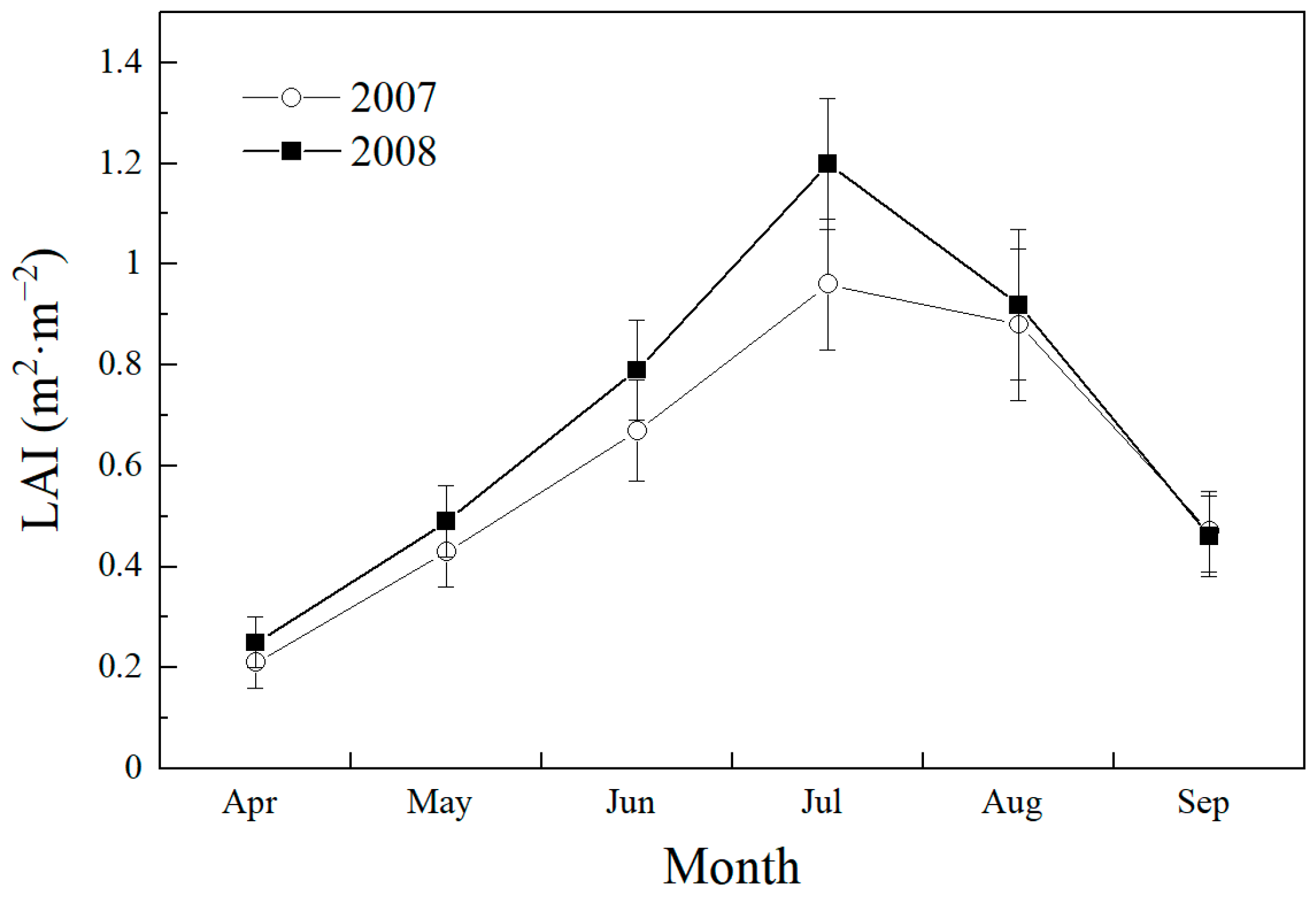
3.1. Variation of LAI and Environmental Variables

The leaf area index (LAI) in both years started to increase from May and reached its annual maximum in July, then decreased rapidly because plants began to senesce in September (Figure 1). The LAI in 2008 was higher than that in 2007, with the maximum values of 1.20 (2008) and 0.96 (2007) m²·m⁻², respectively.

There were no significant differences in annual variation for each environmental variable for the study period (Figure 2), and the corresponding statistical values in the growing season (May–September) and non-growing season are listed in

Table 1. Comparison of environmental conditions during the growing and non-growing seasons at the study site.

Year	Growing Phase	Rn (MJ·m−2·d−1)	G (MJ·m−2·d−1)	Ta (°C)	Ts5cm (°C)	P (mm)	SWC5cm (m3·m−3)	D (kPa)
2006	16 Sept.–31 Dec.	4.43	−0.38	−3.8	1.1	56.3	0.15	0.44
2007	Annual	8.09	0.11	0.2	3.9	493.0	0.18	0.58
	Growing season	12.24	0.47	7.1	10.2	439.7	0.24	0.67
	Non-growing season	5.09	−0.15	−4.8	−0.7	53.3	0.13	0.51
2008	Annual	8.03	−0.05	−0.6	3.1	480.4	0.17	0.51
	Growing season	11.71	0.39	6.6	9.4	417.6	0.24	0.64
	Non-growing season	5.39	−0.36	−5.7	−1.5	62.8	0.13	0.41

R_n, net radiation; G, soil heat flux; T_a, air temperature; T_s5cm, 5 cm soil temperature; SWC_5cm, 5 cm soil water content; D, vapor pressure deficit.

. The annual maximum value of daily net radiation (R_n) appeared in June with 21.23 and 22.07 MJ·m⁻²·d⁻¹ for 2007 and 2008, respectively, and reached the minimum value in winter. The annual R_n in 2007 and 2008 was 2952.11 and 2939.99 MJ·m⁻², respectively, and more than 60% was received during the growing season. The annual variation of soil heat flux (G) followed the same trend of R_n with higher and lower values recorded during the growing and non-growing seasons (Figure 2b), respectively, but it fluctuated within a relatively narrow range from −3.06 to 2.27 MJ·m⁻²·d⁻¹.

The annual variations of air temperature (T_a) and 5 cm soil temperature (T_s5cm) were strongly dependent on R_n, however, T_s5cm was obviously higher than T_a throughout the whole year although T_a followed the same trend as T_s5cm (Figure 2c). The annual mean of T_a was 0.2 °C and −0.6·°C, while the value of T_s5cm was 3.9·°C and 3.1·°C for 2007 and 2008, respectively.

Precipitation occurred mainly during the growing season (Figure 2d), which accounted for 89% and 87% of annual precipitation in 2007 and 2008, respectively. The mean daily precipitation was 2.9 mm·d⁻¹ and 2.7 mm·d⁻¹ during the growing season in 2007 and 2008, respectively, while it was only 0.3 mm·d⁻¹ in the non-growing season for both years. The highest monthly precipitation appeared in June for 2007 and 2008, with the value of 147.5 mm and 101.7 mm, respectively. There was a significant variation in SWC_5cm during the growing season (Figure 2d), which was strongly influenced by precipitation events and ET. This increased rapidly after the occurrence of rainfall and decreased due to E and T when no precipitation occurred. SWC_5cm varied with a range of 0.13–0.32 and 0.17–0.32 m³·m⁻³ during the growing season in 2007 and 2008 with a higher value in June to August, respectively.

Vapor pressure deficit (D) (calculated between 11:30 and 15:30 Beijing Standard Time (BST)) varied within a narrow range between from 0.03 to 1.64 kPa for the study period (Figure 2e). No significant difference was noted for the annual variation trend of D between 2007 and 2008, and overall D exhibited a relatively higher value in May and lower value in January.

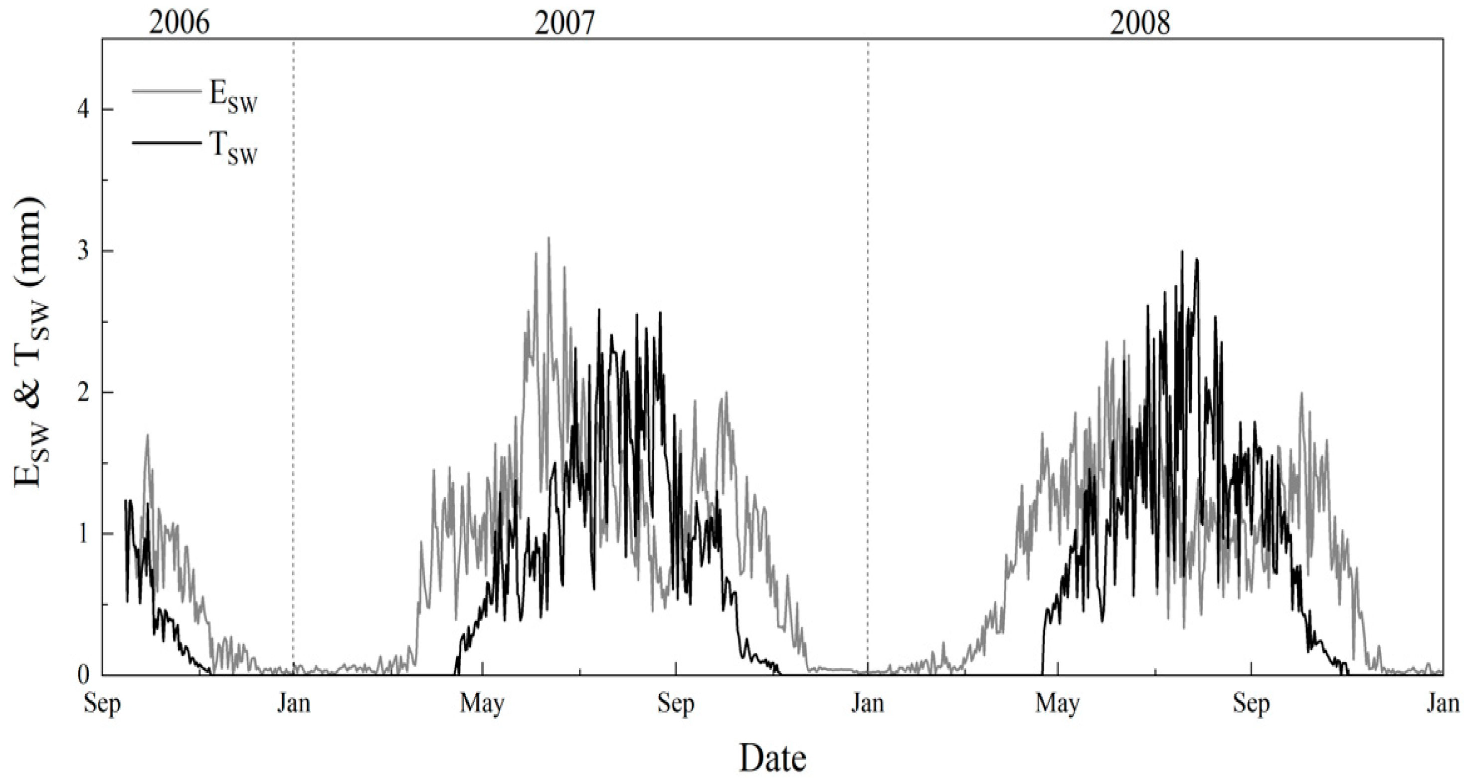
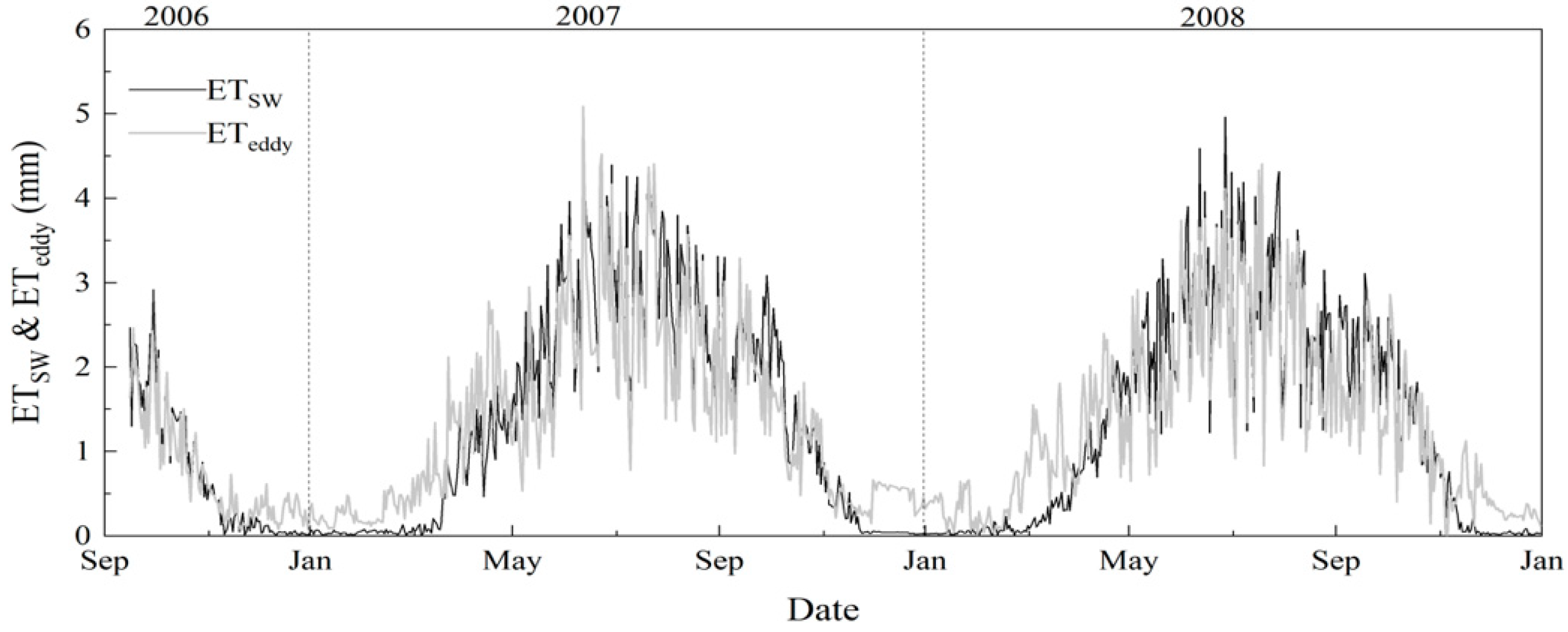
3.2. Annual Variation of ET

Annual change of modeled evapotranspiration (ET_SW) approximately followed the same trend as R_n (Figure 3) and showed a large day to day variation during the growing season. ET_SW started to increase from March and reached its highest annual value around July, and then decreased to the lowest value around January. The majority of ET_SW occurred during the growing season, which was 409.9 mm and 395.3 mm in 2007 and 2008, accounting for 80% and 79% of annual ET_SW, respectively (

Table 2. Evapotranspiration partitioning during the study period.

Year	Growing Phase	ESW (mm)	TSW (mm)	ETSW (mm)
2006	16 Sept.–31 Dec.	51.1	24.2	75.3
2007	Annual	306.0	205.5	511.5
	Growing season	217.6	192.3	409.9
	Non-growing season	88.4	13.2	101.6
2008	Annual	281.7	218.1	499.8
	Growing season	188.1	207.2	395.3
	Non-growing season	93.6	10.9	104.5

).

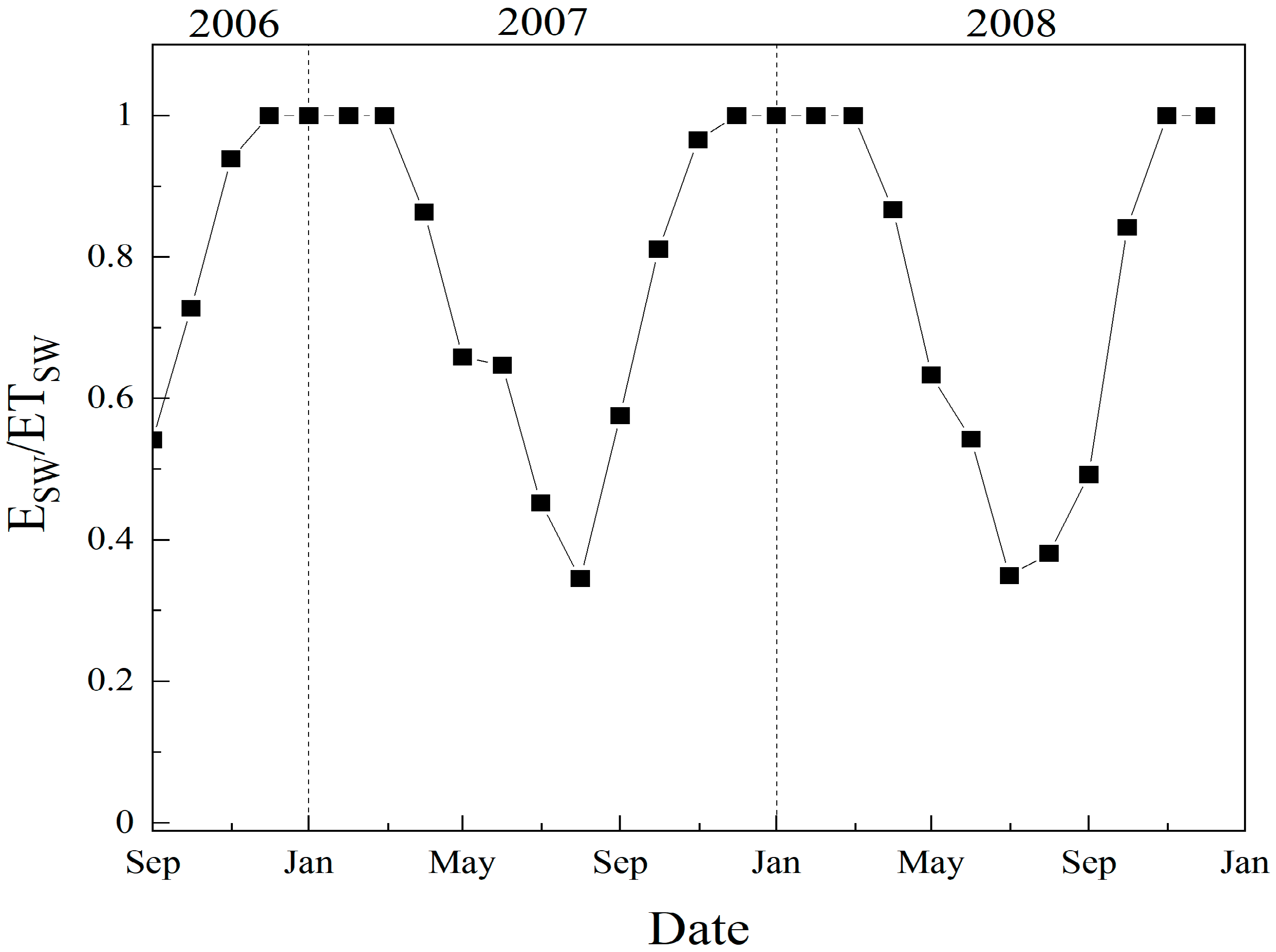
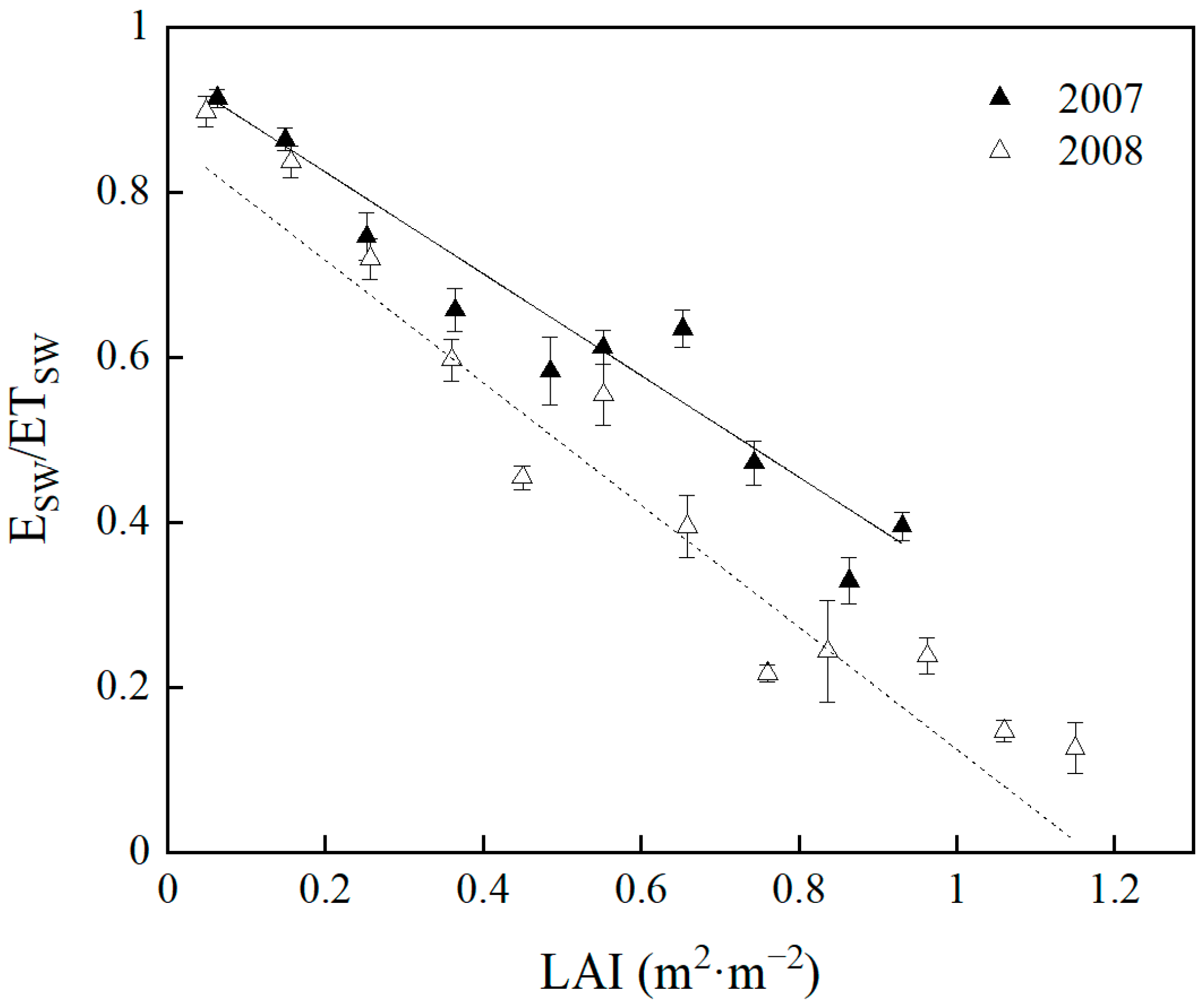
3.3. Evapotranspiration Partitioning

There was an obvious difference between seasonal variations in modeled evaporation (E_SW) and transpiration (T_SW) during the study period (Figure 4). E_SW increased rapidly from early March, reached its maximum value of 3.1 mm (2007) and 2.4 mm (2008) in June, then started to decrease, whereas a relatively lower value was observed in July and August of the growing season. After that, E_SW began to increase again with a second peak appearing around October, and then decreased rapidly from late October. T_SW in both 2007 and 2008 increased from late April when plants started to grow, with the maximum value in July and/or August when E_SW had a relatively lower level. Then, T_SW decreased to its minimum value in late October. The annual amount of E_SW and T_SW accounted for about 60% and 40% of ET_SW in 2007, while the values were 56% and 44% in 2008, respectively. During the growing season, the amount of E_SW and T_SW in 2007 (2008) accounted for 53% (48%) and 47% (52%) of ET_SW, respectively, indicating that soil evaporation was higher than plant transpiration, even though the vegetation was fully developed (for more details see Table 2).

To further explore the influence of E_SW and T_SW on the ET_SW, we analyzed the monthly dynamics of E_SW/ET_SW of the degraded meadow throughout the study period (Figure 5). During the period from November to April of the next year, ET_SW was accounted for by the E_SW (i.e., E_SW/ET_SW = 1.0) because the growth of plants stopped. E_SW/ET_SW gradually decreased from May with the plant growth and reached its minimum value of 0.35 (in August 2007 and in July 2008), then E_SW/ET_SW increased again until November. The average monthly E_SW/ET_SW was 0.50 during the growing season.

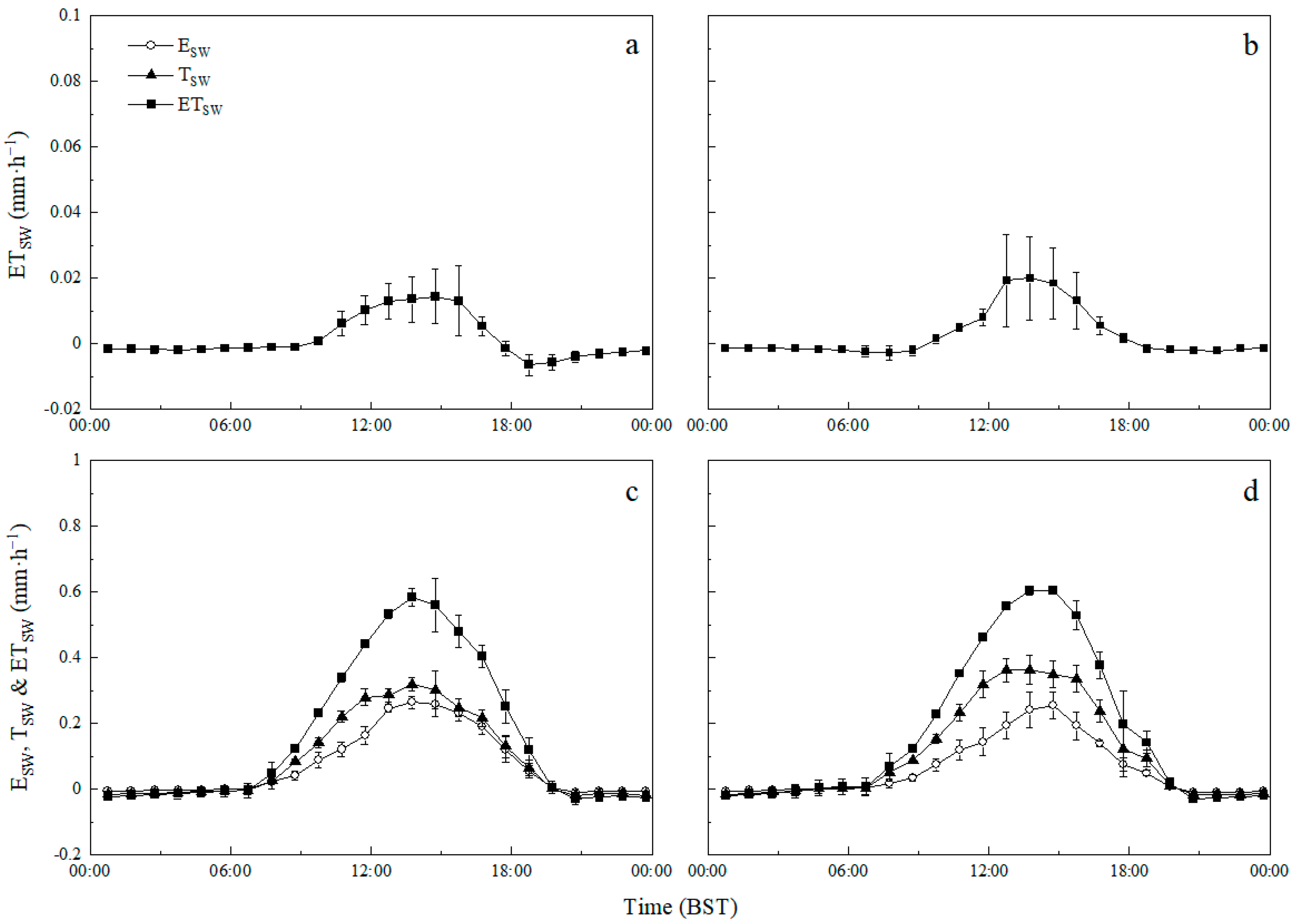
3.4. Diurnal Variation of ET

Diurnal variations of E_SW, T_SW, and ET_SW of clear days in January and July (used to represent winter and summer extreme conditions, respectively) for 2007 and 2008 are shown in Figure 6, where a clear day is defined as that on which the daily transmissivity was greater than 0.7 [18]. All three variables showed the same variation pattern for the two years of 2007 and 2008. In January, ET_SW began to increase around 09:00 and peaked between 13:00 and 15:00 with the maximum average value of about 0.02 mm·h⁻¹, then began to decrease and fell to nearly zero at around 19:00 for both years. In July, however, ET_SW began to increase around 07:00 and reached the maximum at about 14:00, then decreased to about zero at 21:00. Although the ET_SW showed a similar pattern for July and January, the maximum average value of the former with about 0.6 mm·h⁻¹, which was much higher than that of the latter. In addition, it was found that daily T_SW was higher than E_SW in July in both 2007 and 2008 (especially in 2008). In July, daily E_SW with the value of 1.8 mm in 2007 was higher than that of 1.5 mm in 2008, and the daily ratio of E_SW to T_SW (E_SW/T_SW) was 0.80 in 2007, which was higher than that of 0.58 in 2008, while the daily ratio of E_SW to ET_SW (E_SW/ET_SW) was 0.44 and 0.37 in 2007 and 2008, respectively. In other words, the contribution of E_SW to ET_SW in 2007 was higher than that in 2008 in July of the growing season.

4. Discussion

Our simulation results indicated that E accounts for a major part of ET due to vegetation degradation. For environmental (biotic and abiotic) factors that may affect ET and its partitioning, and for the model validation, our research showed the following results:

• E/ET in our research site was more sensitive to change in LAI. E/ET decreased rapidly with the increase of LAI (paragraph 1 in Section 4.1);
• Grassland ecosystems with lower LAI and/or vegetation coverage may lose more water through ET (paragraph 2 in Section 4.1).
• Net. radiation had little effect on ET partitioning, but had a great influence on ET, E, and T (paragraph 2 in Section 4.2).
• Air temperature had a greater effect on T than on E (paragraph 3 in Section 4.2).
• Soil water content at a 5 cm depth affected both ET and ET partitioning in this degraded meadow, especially for the E (paragraph 4 in Section 4.2).
• Vapor pressure deficit had little effect on both ET and ET partitioning (paragraph 5 in Section 4.2).
• Leaf area index is an important factor influencing ET partitioning (paragraph 6 in Section 4.2).
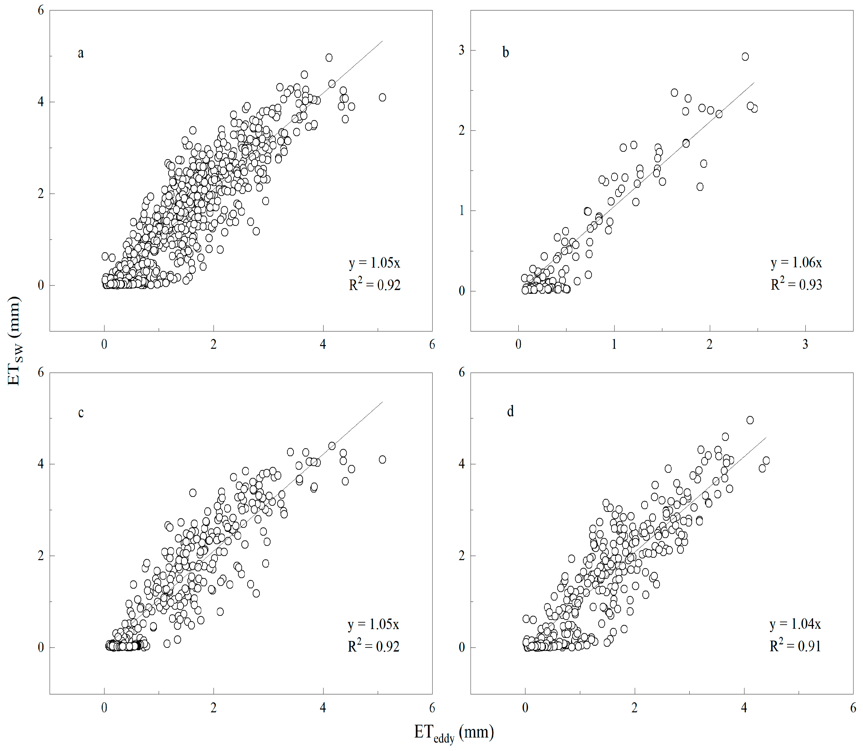
• The model results had good agreement with the ET observed by the eddy covariance system (paragraph 2 in Section 4.3).

4.1. Effects of Vegetation on Evapotranspiration Partitioning

ET is mainly dependent on vegetation, meteorological conditions, and soil water [37], and the partitioning of ET into E and T is strongly influenced by changes in vegetation characteristics during the growing season [38,39]. Leaf area index (LAI) is often used to quantify terrestrial ecosystem ET as well as ET partitioning; an increase in leaf area will initially increase ET when the soil water content is high, and this response will weaken at high LAI [40,41]. In this degraded meadow, the variation pattern of E is quite different from that of T during the growing season (Figure 4). Seasonal variation of T followed the same trend of LAI, with the higher values recorded around August at higher LAI (Figure 1), however, the highest E occurred around June. The result is consistent with many literature reports [39,42,43]. The analysis of the relationship between LAI and E/ET during the growing season is illustrated in Figure 7. The E/ET data were LAI-bin averaged because this data compilation helped to reduce or offset the errors associated with the measurements [34]. The LAI gaps were linearly interpolated to daily intervals [44]. It was found that there was a significant negative correlation between E/ET and LAI for 2007 and 2008 (Figure 7) (i.e., the contribution of soil evaporation to evapotranspiration decreased linearly with the increase in LAI), which is consistent with other alpine meadow ecosystems reported by [17]. A previous study also reported a similar negative relationship in multiple ecosystems (e.g., forests, crops, wetlands, shrubs, and grasses) [45]. Several studies have reported that E/ET initially decreased rapidly with an increase in LAI at the low vegetative cover (low LAI), while the response of E/ET to LAI decreased gradually with the increasing LAI, and finally approached a constant value [14,17,43,45]. In the present study, however, the LAI was very low, even in the peak growing season, with the maximum value of 1.20 m²·m⁻² (July 2008) due to the meadow degradation, therefore, E/ET was more sensitive to change in LAI. Based on the diurnal variation of ET partitioning in the peak growing season of July (Figure 6), the daily E/ET in 2007 was obviously higher than that in 2008 due to the relatively high LAI in 2008 compared with 2007. In addition, E in the growing season of 2007 was higher than that of 2008 whereas the opposite result was obtained for T (Table 2), and the regression line between E/ET and LAI for 2007 was above that for 2008, indicating that the contribution of E to ET in 2007 was higher than that in 2008, which may be due to the lower LAI for 2007 compared with 2008 that resulted in the increase in ET of this alpine meadow (Table 2).

To further investigate the relationship between vegetation and ET partitioning, we made a comparison between our results and some of the previously published studies on grassland ecosystems (

Table 3. Comparison between E/ET, T/ET, ET/P, and vegetation conditions observed in the degraded meadow and values observed in other grassland ecosystems.

Location	Study Period	E/ET (%)	T/ET (%)	ET/P (%)	Vegetation Type	Coverage (%)	Maximum LAI (m2·m−2)	References
37°36′ N, 101°18′ E, 3250 m a.s.l	2002–2004	-	-	56–61	alpine meadow	>90	3	[9]
37°37′ N, 101°20′ E, 3160 m a.s.l.	2003–2005	40–43	57–60	-	alpine meadow	70–80	4	[17]
37°40′ N, 101°20′ E, 3293 m a.s.l	2003–2005	36–45	55–64	-	alpine meadow	70–80	2.8	[17]
30°51′ N, 91°05′ E, 4333 m a.s.l.	2004–2005	56–60	40–44	-	alpine meadow-steppe	45–55	1.1	[17]
43°33′ N, 116°40′ E, 1252 m a.s.l.	2003–2004	57–61	39–43	-	temperate steppe	60–70	1.5	[17]
42°02′48′′ N, 116°17′01′′ E, 1350 m a.s.l	2005–2006	-	-	89	typical steppe	-	0.47	[46]
43°33′16′′ N, 116°40′17′′ E, 1250 m a.s.l	2005–2006	-	-	107	degraded steppe	-	0.25	[46]
44°25′ N, 122°52′ E, 184 m a.s.l	2003–2008	-	-	97–101	degraded grassland	<70	-	[47]
31.9083° N, 110.8395° W, 1000 m a.s.l	summer 2008	63	37	104	shrubland	24	0.55	[7]
31.7438° N, 110.0522° W, 1375 m a.s.l	summer 2008	56	44	92	shrubland	27	0.66	[7]
43°40′26.61′′ S, 171°35′27.63′′ E, 309 m a.s.l	2011–2012	25	75	78	pasture	-	5–6	[48]
31.737° N, 109.942° W, 1531 m a.s.l	2005–2018	-	35–46	91	grassland	-	0.56–1.80	[49]
34°24′ N, 100°24′ E, 3963 m a.s.l	2006–2008	48–53	47–52	93–95	degraded alpine meadow	55	1.20	In this study

E/ET, the ratio of soil evaporation to evapotranspiration; T/ET, the ratio of plant transpiration to evapotranspiration; ET/P, the ratio of evapotranspiration to precipitation.

). All of these studies reported a negative relationship between vegetation conditions and E/ET, which is consistent with our research. However, it is worth noting that worse vegetation conditions corresponded to higher ET/P (the ratio of evapotranspiration to precipitation) (Table 3). We suggest that this is due to the degradation of vegetation thus allowing more energy to reach the soil surface, which leads to increased E and ET. Furthermore, Gu et al. [9] found a curve relationship between the aboveground biomass and ET at an alpine meadow ecosystem. That is, ET increased gradually with the increase in aboveground biomass at first, but decreased thereafter despite the biomass still increasing.

4.2. Effects of Environmental Factors on Evapotranspiration Partitioning

Except for the vegetation LAI, solar radiation, temperature, soil moisture, and air humidity will also have an impact on the partitioning of evapotranspiration [9,10,50,51]. Consequently, to comprehensively understand the control of environmental factors on the balance between evaporation and transpiration, net radiation (R_n), air temperature (T_a), 5 cm soil water content (SWC_5cm), vapor pressure deficit (D) as well as the leaf area index (LAI) were chosen to analyze the effects of the above factors on the ET and its partitioning (E/ET and T/ET). In this study, we referred to the method by [42], where each dependent variable was multiplied by 0.5 and 2.0 in the model, respectively, then the model was rerun to see how much the output value changed (Figure 8 and

Table 4. Effects of net radiation (R_n), air temperature (T_a), 5 cm soil water content (SWC_5cm), vapor pressure deficit (D) and leaf area index (LAI) on ET, E, and T in the growing season of 2007 and 2008 for the degraded meadow.

Input Variables	Percentage of Variation
	−50%			+100%
	ETSW	ESW	TSW	ETSW	ESW	TSW
Net radiation, Rn (MJ·m−2)	−66%	−66%	−67%	+133%	+132%	+133%
Air temperature, Ta (°C)	−13%	−9%	−16%	+22%	+11%	+33%
5 cm soil water content, SWC5cm (m3·m−3)	−14%	−62%	+35%	+9%	+41%	−22%
Leaf area index, LAI (m2·m−2)	−3%	+38%	−45%	+4%	−46%	+54%
Vapor pressure deficit, D (kPa)	−<1%	−<1%	−<1%	+<1%	+<1%	+<1%

). Here, multiplying by 0.5 and 2.0 is defined as “low level” and “high level”, respectively, and “standard” is the observed value.

Solar radiation is the most important source of energy for most biological and meteorological processes, and ET, E, and T are dependent mainly on the solar energy available to vaporize the water [50]. It was found that R_n had little effect on ET partitioning (E/ET and T/ET) (Figure 8a), but had a great influence on ET, E, and T (Table 4), which is consistent with previous research results [50]. ET, E, and T were decreased about 66% compared with the standard when R_n was at a low level and increased about 132% when R_n was doubled (Table 4). The results suggest that the change of R_n strongly influences ET, E, and T, but there was almost no influence on E/ET and T/ET in this degraded meadow ecosystem.

Temperature is one of the major factors affecting the rate of ET, E, and T, and temperature-based models are widely used to estimate ET [51,52]. Our results showed that E/ET was slightly higher (or lower) than the standard when T_a was at a low level (or high level), while an opposite change was found for T/ET (Figure 8b). However, T_a had a positive relationship with ET, E, and T (Table 4), and the effect of T_a on T was greater than ET and E (Table 4). In this study, the variation of T almost followed the same trend of LAI and T_a with a higher value in about July (Figure 1, Figure 2c and Figure 4), indicating that T increased with the increase in LAI and T_a, but E decreased rapidly with the increasing LAI, therefore the response of T to T_a was more sensitive compared with the E.

Numerous studies have shown that ecosystem ET is closely related to the soil water content [10,25,47]. Our results indicated that SWC_5cm affected both ET and its partitioning in this degraded meadow, especially for the E (Figure 8d, Table 4). It was observed that E/ET and T/ET showed the opposite change trend when the SWC_5cm was multiplied by 0.5 and 2 (Figure 8d), respectively, in which increasing SWC_5cm significantly increased E/ET and decreased T/ET, and the converse was also true (Figure 8d). Soil water content is an important factor controlling soil surface resistance, and increasing SWC_5cm can reduce bare soil surface resistance to evaporation, and at the same time, increase the supply of soil moisture, resulting in an increase of E and E/ET. The previous study pointed out that transpiration will increase rapidly with the increase in soil water content when water supply is limited [53], which is inconsistent with our results. However, transpiration is strongly dependent not only on the soil water content, but also on meteorological and vegetation conditions. In this alpine meadow, most of the root system was distributed within the 0 to 10 cm surface layer, and the soil maintained a relatively high-water content throughout the growing season due to the abundant precipitation (Figure 2d), while a downward trend of SWC_5cm was observed in the peak growing season of July–August due to the high ET. Therefore, under the condition that other observed variables are included in the model, our results showed that T and T/ET decreased when only increasing SWC_5cm, and the possible reason is that T is predominantly controlled by R_n and LAI, and at the same time, affected by the SWC_5cm. The model result is consistent with the actual change in transpiration, and a similar relationship was also observed between the T and SWC_5cm in another study by using micro-lysimeter experiments in an alpine meadow of the TRSR (article in print).

Vapor pressure deficit (D) is one of the principal weather variables affecting ET because D affects the evaporation demand of the atmosphere and canopy conductance [9]. Our results showed that D had a very small effect on both ET and its partitioning (Figure 8c, Table 4), perhaps because the value of measured D was very low and varied within a very narrow range from 0.03 to 1.64 kPa in this degraded meadow (Figure 2e), which was significantly lower than many other grassland values with the maximum D ranging from about 2 to 5 kPa [4]. Thus, when D was multiplied by 0.5 and 2.0, there was almost no change in ET as well as its partitioning.

LAI is one of the important parameters describing vegetation characteristics, which is widely adopted in ET partitioning [6,39]. The simulation results showed that E/ET will increase or decrease significantly compared with the “standard” level when LAI is multiplied by 0.5 or 2.0, while in contrast, an opposite trend was observed for T/ET with increasing or decreasing LAI (Figure 8e) and it was also noted that there was the same trend for E and T (Table 4). Our results are consistent with earlier studies that showed the effects of LAI on ET partitioning [41,45]. However, the effect of LAI on ET was relatively small because the E pattern was almost the opposite to that of T during the growing season (Figure 4), so increasing E may be offset by the decreasing T. Usually, increasing LAI can increase vegetation cover and lead to a decrease in bare soil surface area, then decreases E and/or increases T, and the reverse is also true.

Overall, LAI and SWC_5cm are the main important factors influencing E/ET and/or T/ET. E and T were primarily controlled by R_n, LAI, and SWC_5cm, while the effect of T_a on T was relatively large compared with E. D had little effect on both ET and ET partitioning.

4.3. Validation of the Shuttleworth–Wallace Model

The eddy covariance (EC) system was conducted in our flat degraded meadow. The WPL density correction was applied to water vapor flux [54], and the energy balance ratio (EBR) was calculated using the following equation [55]:

$$EBR=\frac{{{\displaystyle \sum }}^{ }\left(LE+H\right)}{{{\displaystyle \sum }}^{ }\left(R_n-G\right)}$$

(7)

where H, LE, and G are the sensible, latent, and soil heat fluxes. In this study, the term (LE + H), measured by the EC method, seemed to be underestimated since the average value of EBR was 0.79 in the study period, which fell in the median region of reported energy closures, which ranged from 0.55 to 0.99 [55]. LE was converted to ET (mm) by assuming a value for a conversion factor of 2450 J/g.

In order to verify the performance of the S–W model over the alpine meadow, we compared the ET estimated by the S–W model (ET_SW) to that measured by the EC method (ET_eddy) (Figure 9). Overall, there was a good agreement between ET_SW and ET_eddy in the study period, while the ET_SW was underestimated compared to the ET_eddy from December to April of the next year (Figure 9). Gong et al. [56] also pointed out that the S–W model overestimated and/or underestimated ET at different growth stages in comparison with the results measured by the lysimeter. Therefore, we performed some statistical analyses between ET_SW and ET_eddy in the growing and non-growing seasons (

Table 5. Statistical analyses of evapotranspiration estimated by the S–W model (ET_SW) and measured by the eddy covariance (ET_eddy) in the different periods.

Year	Period	k	R2	RMSE	MAE
2006	16 September–31 December	1.06	0.93	0.3	0.2
2007	Annual	1.05	0.92	0.5	0.4
	Growing season	1.13	0.96	0.6	0.5
	Non-growing season	0.71	0.76	0.5	0.4
2008	Annual	1.04	0.91	0.6	0.4
	Growing season	1.12	0.96	0.6	0.5
	Non-growing season	0.72	0.74	0.5	0.4

k, slope (dimensionless); R², determination coefficient; RMSE, root mean square (mm·d⁻¹); MAE, mean absolute error (mm·d⁻¹).

). It was found that the model performance in the growing season was better than that in the non-growing season, and the model overestimation of ET occurred in the growing season, while the underestimation appeared in the non-growing season. The relationships between ET_SW and ET_eddy at different growth stages for 2006–2008 were summarized through statistical analyses (Figure 10 and Table 5). The linear regression slopes (k) ranged from 1.04 to 1.06 and the values of R² (square of the correlation coefficient) were over 0.91. RMSE and MAE varied in the range of 0.3–0.6 and 0.2–0.5 mm·d⁻¹, respectively. The possible reason for this overestimation of ET might be due to the lack of energy balance closure of the eddy covariance method (EBR = 0.79), and thus the ET was underestimated by the EC method. Chen et al. [37] reported that the S–W model overestimated ET by comparing it with the measured data. Wei et al. [57] indicated that the S–W model overestimated ET by 5% when compared to the measured data, which is similar to our simulation results. On the whole, the ET was well estimated by the S–W model in this degraded meadow on the Qinghai-Tibetan Plateau.

5. Conclusions

We estimated evapotranspiration (ET) and its partitioning with the S–W model in a degraded alpine meadow in the TRSR, and compared the results with data obtained from eddy covariance. The validation confirmed the good performance of the S–W model for the prediction of ET and its partitioning in this study. Net radiation is the most important factor influencing ET while leaf area index (LAI) is a key factor affecting ET partitioning. Due to the vegetation degradation at our research site, the contribution of soil evaporation (E) accounted for the main part of ET, and ET was higher with the lower LAI. Our results suggest that the water lost by ET from the meadow ecosystem increased with the increasing intensity of vegetation degradation, that is, meadow degradation would increase water loss through increasing E, leading to reducing the water conservation capacity of the alpine meadow ecosystem in TRSR.

References

1. Garratt, J.R. Sensitivity of Climate Simulations to Land-Surface and Atmospheric Boundary-Layer Treatments-A Review. J. Clim. 1993, 6, 419–448. [Google Scholar] [CrossRef] [Green Version]
2. Wang, K.; Dickinson, R.E. A review of global terrestrial evapotranspiration: Observation, modeling, climatology, and climatic variability. Rev. Geophys. 2012, 50, RG2005. [Google Scholar] [CrossRef]
3. Trenberth, K.E.; Smith, L.; Qian, T.; Dai, A.; Fasullo, J. Estimates of the Global Water Budget and Its Annual Cycle Using Observational and Model Data. J. Hydrometeorol. 2007, 8, 758–769. [Google Scholar] [CrossRef]
4. Wever, L.A.; Flanagan, L.B.; Carlson, P.J. Seasonal and interannual variation in evapotranspiration, energy balance and surface conductance in a northern temperate grassland. Agric. For. Meteorol. 2002, 112, 31–49. [Google Scholar] [CrossRef]
5. Williams, D.; Cable, W.; Hultine, K.; Hoedjes, J.; Yepez, E.; Simonneaux, V.; Er-Raki, S.; Boulet, G.; de Bruin, H.; Chehbouni, A.; et al. Evapotranspiration components determined by stable isotope, sap flow and eddy covariance techniques. Agric. For. Meteorol. 2004, 125, 241–258. [Google Scholar] [CrossRef]
6. Scott, R.L.; Huxman, T.E.; Cable, W.L.; Emmerich, W.E. Partitioning of evapotranspiration and its relation to carbon dioxide exchange in a Chihuahuan Desert shrubland. Hydrol. Process. 2006, 20, 3227–3243. [Google Scholar] [CrossRef] [Green Version]
7. Cavanaugh, M.L.; Kurc, S.A.; Scott, R. Evapotranspiration partitioning in semiarid shrubland ecosystems: A two-site evaluation of soil moisture control on transpiration. Ecohydrology 2010, 4, 671–681. [Google Scholar] [CrossRef]
8. Hu, Z.; Li, S.; Yu, G.; Sun, X.; Zhang, L.; Han, S.; Li, Y. Modeling evapotranspiration by combing a two-source model, a leaf stomatal model, and a light-use efficiency model. J. Hydrol. 2013, 501, 186–192. [Google Scholar] [CrossRef]
9. Gu, S.; Tang, Y.H.; Cui, X.Y.; Du, M.Y.; Zhao, L.; Li, Y.N.; Xu, S.X.; Zhou, H.K.; Kato, T.; Qi, P.T.; et al. Characterizing evapotranspiration over a meadow ecosystem on the Qinghai-Tibetan Plateau. J. Geophys Res. Atmos. 2008, 113, D8. [Google Scholar] [CrossRef]
10. Giambelluca, T.W.; Scholz, F.G.; Bucci, S.J.; Meinzer, F.; Goldstein, G.; Hoffmann, W.A.; Franco, A.; Buchert, M. Evapotranspiration and energy balance of Brazilian savannas with contrasting tree density. Agric. For. Meteorol. 2009, 149, 1365–1376. [Google Scholar] [CrossRef]
11. Wang, B.; Jin, H.Y.; Li, Q.; Chen, D.D.; Zhao, L.; Tang, Y.H.; Kato, T.; Gu, S. Diurnal and seasonal variations in the net ecosystem CO2 exchange of a pasture in the three-river source region of the Qinghai−Tibetan Plateau. PLoS ONE 2017, 12, e0170963. [Google Scholar] [CrossRef]
12. Kool, D.; Agam, N.; Lazarovitch, N.; Heitman, J.L.; Sauer, T.J.; Ben-Gal, A. A review of approaches for evapotranspiration partitioning. Agric. For. Meteorol. 2014, 184, 56–70. [Google Scholar] [CrossRef]
13. Shuttleworth, W.J.; Wallace, J.S. Evaporation from sparse crops-an energy combination theory. Q. J. R. Meteorol. Soc. 1985, 111, 839–855. [Google Scholar] [CrossRef]
14. Brisson, N.; Itier, B.; L’Hotel, J.C.; Lorendeau, J.Y. Parameterisation of the Shuttleworth-Wallace model to estimate daily maximum transpiration for use in crop models. Ecol. Model. 1998, 107, 159–169. [Google Scholar] [CrossRef]
15. Ortega-Farias, S.; Carrasco, M.; Olioso, A.; Acevedo, C.; Poblete-Echeverría, C. Latent heat flux over Cabernet Sauvignon vineyard using the Shuttleworth and Wallace model. Irrig. Sci. 2006, 25, 161–170. [Google Scholar] [CrossRef]
16. Zhao, P.; Li, S.; Li, F.; Du, T.; Tong, L.; Kang, S. Comparison of dual crop coefficient method and Shuttleworth–Wallace model in evapotranspiration partitioning in a vineyard of northwest China. Agric. Water Manag. 2015, 160, 41–56. [Google Scholar] [CrossRef]
17. Hu, Z.; Yu, G.; Zhou, Y.; Sun, X.; Li, Y.; Shi, P.; Wang, Y.; Song, X.; Zheng, Z.; Zhang, L.; et al. Partitioning of evapotranspiration and its controls in four grassland ecosystems: Application of a two-source model. Agric. For. Meteorol. 2009, 149, 1410–1420. [Google Scholar] [CrossRef]
18. Gu, S.; Tang, Y.; Cui, X.; Kato, T.; Du, M.; Li, Y.; Zhao, X. Energy exchange between the atmosphere and a meadow ecosystem on the Qinghai–Tibetan Plateau. Agric. For. Meteorol. 2005, 129, 175–185. [Google Scholar] [CrossRef]
19. You, Q.; Xue, X.; Peng, F.; Dong, S.; Gao, Y. Surface water and heat exchange comparison between alpine meadow and bare land in a permafrost region of the Tibetan Plateau. Agric. For. Meteorol. 2017, 232, 48–65. [Google Scholar] [CrossRef]
20. Gu, S.; Tang, Y.H.; Du, M.Y.; Kato, T.; Li, Y.N.; Cui, X.Y.; Zhao, X.Q. Short-term variation of CO2 flux in relation to environmental controls in an alpine meadow on the Qinghai-Tibetan Plateau. J. Geophys Res. Atmos. 2003, 108, D21. [Google Scholar] [CrossRef]
21. Yao, T.; Thompson, L.G.; Mosbrugger, V.; Zhang, F.; Ma, Y.; Luo, T.; Xu, B.; Yang, X.; Joswiak, D.R.; Wang, W.; et al. Third Pole Environment (TPE). Environ. Dev. 2012, 3, 52–64. [Google Scholar] [CrossRef]
22. Zhang, G.; Zhang, Y.; Dong, J.; Xiao, X. Green-up dates in the Tibetan Plateau have continuously advanced from 1982 to 2011. Proc. Natl. Acad. Sci. USA 2013, 110, 4309–4314. [Google Scholar] [CrossRef] [Green Version]
23. Guo, B.; Zhou, Y.; Zhu, J.; Liu, W.; Wang, F.; Wang, L.; Yan, F.; Wang, F.; Yang, G.; Luo, W.; et al. Spatial patterns of ecosystem vulnerability changes during 2001–2011 in the three-river source region of the Qinghai-Tibetan Plateau, China. J. Arid. Land 2015, 8, 23–35. [Google Scholar] [CrossRef]
24. Qu, B.; Sillanpää, M.; Kang, S.; Yan, F.; Li, Z.; Zhang, H.; Li, C. Export of dissolved carbonaceous and nitrogenous substances in rivers of the “Water Tower of Asia”. J. Environ. Sci. 2018, 65, 53–61. [Google Scholar] [CrossRef] [PubMed]
25. Zhang, X.; Liu, X.Q.; Zhang, L.F.; Chen, Z.G.; Zhao, L.; Li, Q.; Chen, D.D.; Gu, S. Comparison of energy partitioning between artificial pasture and degraded meadow in three-river source region on the Qinghai-Tibetan Plateau: A case study. Agric. For. Meteorol. 2019, 271, 251–263. [Google Scholar] [CrossRef]
26. Chen, F.; Zhang, J.; Liu, J.; Cao, X.; Hou, J.; Zhu, L.; Xu, X.; Liu, X.; Wang, M.; Wu, D.; et al. Climate change, vegetation history, and landscape responses on the Tibetan Plateau during the Holocene: A comprehensive review. Quat. Sci. Rev. 2020, 243, 106444. [Google Scholar] [CrossRef]
27. Liu, X.; Zhang, J.; Zhu, X.; Pan, Y.; Liu, Y.; Zhang, D.; Lin, Z. Spatiotemporal changes in vegetation coverage and its driving factors in the Three-River Headwaters Region during 2000–2011. J. Geogr. Sci. 2014, 24, 288–302. [Google Scholar] [CrossRef]
28. Liu, J.; Xu, X.; Shao, Q. Grassland degradation in the “three-river headwaters” region, Qinghai province. J. Geogr. Sci. 2008, 18, 259–273. [Google Scholar] [CrossRef]
29. Feng, J.; Wang, T.; Qi, S.; Xie, C. Land degradation in the source region of the Yellow River, northeast Qinghai-Xizang Plateau: Classification and evaluation. Environ. Earth Sci. 2004, 47, 459–466. [Google Scholar] [CrossRef]
30. Zhang, Y.; Zhang, S.; Zhai, X.; Xia, J. Runoff variation and its response to climate change in the Three Rivers Source Region. J. Geogr. Sci. 2012, 22, 781–794. [Google Scholar] [CrossRef]
31. Li, H.; Liu, G.; Fu, B. Estimation of regional evapotranspiration in alpine area and its response to land use change: A case study in Three-River Headwaters region of Qinghai-Tibet Plateau, China. Chin. Geogr. Sci. 2012, 22, 437–449. [Google Scholar] [CrossRef]
32. Zhang, Y.; Zhang, S.; Xia, J.; Hua, D. Temporal and spatial variation of the main water balance components in the three rivers source region, China from 1960 to 2000. Environ. Earth Sci. 2012, 68, 973–983. [Google Scholar] [CrossRef]
33. Zeng, C.; Zhang, F.; Wang, Q.; Chen, Y.; Joswiak, D.R. Impact of alpine meadow degradation on soil hydraulic properties over the Qinghai-Tibetan Plateau. J. Hydrol. 2013, 478, 148–156. [Google Scholar] [CrossRef]
34. Falge, E.; Baldocchi, D.; Olson, R.; Anthoni, P.; Aubinet, M.; Bernhofer, C.; Burba, G.; Ceulemans, R.J.; Clement, R.; Dolman, A.; et al. Gap filling strategies for defensible annual sums of net ecosystem exchange. Agric. For. Meteorol. 2001, 107, 43–69. [Google Scholar] [CrossRef] [Green Version]
35. Zhou, M.C.; Ishidaira, H.; Hapuarachchi, H.P.; Magome, J.; Kiem, A.S.; Takeuchi, K. Estimating potential evapotranspiration using Shuttleworth–Wallace model and NOAA-AVHRR NDVI data to feed a distributed hydrological model over the Mekong River basin. J. Hydrol. 2006, 327, 151–173. [Google Scholar] [CrossRef]
36. Farahani, H.J.; Bausch, W.C. Performance of Evapotranspiration Models for Maize—Bare Soil to Closed Canopy. Trans. ASAE 1995, 38, 1049–1059. [Google Scholar] [CrossRef]
37. Chen, H.; Huang, J.J.; McBean, E. Partitioning of daily evapotranspiration using a modified shuttleworth-wallace model, random Forest and support vector regression, for a cabbage farmland. Agric. Water Manag. 2020, 228, 105923. [Google Scholar] [CrossRef]
38. García-Leoz, V.; Villegas, J.C.; Suescún, D.; Flórez, C.P.; Merino-Martín, L.; Betancur, T.; León, J.D. Land cover effects on water balance partitioning in the Colombian Andes: Improved water availability in early stages of natural vegetation recovery. Reg. Environ. Chang. 2018, 18, 1117–1129. [Google Scholar] [CrossRef]
39. Hu, H.; Chen, L.; Liu, H.; Khan, M.Y.A.; Tie, Q.; Zhang, X.; Tian, F. Comparison of the Vegetation Effect on ET Partitioning Based on Eddy Covariance Method at Five Different Sites of Northern China. Remote Sens. 2018, 10, 1755. [Google Scholar] [CrossRef] [Green Version]
40. Li, S.-G.; Lai, C.-T.; Lee, G.; Shimoda, S.; Yokoyama, T.; Higuchi, A.; Oikawa, T. Evapotranspiration from a wet temperate grassland and its sensitivity to microenvironmental variables. Hydrol. Process. 2004, 19, 517–532. [Google Scholar] [CrossRef]
41. Marques, T.V.; Mendes, K.; Mutti, P.; Medeiros, S.; Silva, L.; Perez-Marin, A.M.; Campos, S.; Lúcio, P.S.; Lima, K.; dos Reis, J.S.; et al. Environmental and biophysical controls of evapotranspiration from Seasonally Dry Tropical Forests (Caatinga) in the Brazilian Semiarid. Agric. For. Meteorol. 2020, 287, 107957. [Google Scholar] [CrossRef]
42. Lauenroth, W.K.; Bradford, J. Ecohydrology and the Partitioning AET between Transpiration and Evaporation in a Semiarid Steppe. Ecosystems 2006, 9, 756–767. [Google Scholar] [CrossRef]
43. Zhu, G.; Su, Y.; Li, X.; Zhang, K.; Li, C. Estimating actual evapotranspiration from an alpine grassland on Qinghai-Tibetan plateau using a two-source model and parameter uncertainty analysis by Bayesian approach. J. Hydrol. 2013, 476, 42–51. [Google Scholar] [CrossRef]
44. Li, S.G.; Eugster, W.; Asanuma, J.; Kotani, A.; Davaa, G.; Oyunbaatar, D.; Sugita, M. Energy partitioning and its biophysical controls above a grazing steppe in central Mongolia. Agric. For. Meteorol. 2006, 137, 89–106. [Google Scholar] [CrossRef]
45. Wei, Z.; Yoshimura, K.; Wang, L.; Miralles, D.G.; Jasechko, S.; Lee, X. Revisiting the contribution of transpiration to global terrestrial evapotranspiration. Geophys. Res. Lett. 2017, 44, 2792–2801. [Google Scholar] [CrossRef] [Green Version]
46. Chen, S.; Chen, J.; Lin, G.; Zhang, W.; Miao, H.; Wei, L.; Huang, J.; Han, X. Energy balance and partition in Inner Mongolia steppe ecosystems with different land use types. Agric. For. Meteorol. 2009, 149, 1800–1809. [Google Scholar] [CrossRef]
47. Liu, H.Z.; Feng, J.W. Seasonal and interannual variations of evapotranspiration and energy exchange over different land surfaces in a semiarid area of China. J. Appl. Meteorol. Climatol. 2012, 51, 1875–1888. [Google Scholar]
48. Graham, S.; Kochendorfer, J.; McMillan, A.; Duncan, M.J.; Srinivasan, M.; Hertzog, G. Effects of agricultural management on measurements, prediction, and partitioning of evapotranspiration in irrigated grasslands. Agric. Water Manag. 2016, 177, 340–347. [Google Scholar] [CrossRef]
49. Scott, R.L.; Knowles, J.F.; Nelson, J.A.; Gentine, P.; Li, X.; Barron-Gafford, G.; Bryant, R.; Biederman, J.A. Water availability impacts on evapotranspiration partitioning. Agric. For. Meteorol. 2021, 297, 108251. [Google Scholar] [CrossRef]
50. Pereira, A.B.; Nova, N.A.V.; Pires, L.F.; Angelocci, L.R.; Beruski, G.C. Estimation method of grass net radiation on the determination of potential evapotranspiration. Meteorol. Appl. 2012, 21, 369–375. [Google Scholar] [CrossRef]
51. Yang, L.; Feng, Q.; Adamowski, J.F.; Yin, Z.; Wen, X.; Wu, M.; Jia, B.; Hao, Q. Spatio-temporal variation of reference evapotranspiration in northwest China based on CORDEX-EA. Atmos. Res. 2020, 238, 104868. [Google Scholar] [CrossRef]
52. Rosenberg, N.J.; Blad, B.L.; Verma, S.B. Evaporation and Evapotranspiration, in Microclimate: The Biological Environment, 2nd ed.; Wiley-Intersci.: New York, NY, USA, 1983; pp. 209–287. [Google Scholar]
53. Novák, V.; Hurtalova, T.; Matejka, F. Predicting the effects of soil water content and soil water potential on transpiration of maize. Agric. Water Manag. 2005, 76, 211–223. [Google Scholar] [CrossRef]
54. Webb, E.K.; Pearman, G.I.; Leuning, R. Correction of flux measurements for density effects due to heat and water vapour transfer. Q. J. R. Meteorol. Soc. 1980, 106, 85–100. [Google Scholar] [CrossRef]
55. Wilson, K.; Goldstein, A.; Falge, E.; Aubinet, M.; Baldocchi, D.; Berbigier, P.; Bernhofer, C.; Ceulemans, R.J.; Dolman, A.; Field, C.; et al. Energy balance closure at FLUXNET sites. Agric. For. Meteorol. 2002, 113, 223–243. [Google Scholar] [CrossRef] [Green Version]
56. Gong, X.; Liu, H.; Sun, J.; Gao, Y.; Zhang, H. Comparison of Shuttleworth-Wallace model and dual crop coefficient method for estimating evapotranspiration of tomato cultivated in a solar greenhouse. Agric. Water Manag. 2019, 217, 141–153. [Google Scholar] [CrossRef]
57. Wei, G.; Zhang, X.; Ye, M.; Yue, N.; Kan, F. Bayesian performance evaluation of evapotranspiration models based on eddy covariance systems in an arid region. Hydrol. Earth Syst. Sci. 2019, 23, 2877–2895. [Google Scholar] [CrossRef] [Green Version]
Figure 1. Variation of leaf area index (LAI) during the growing season in 2007 and 2008.
Water 13 02061 g001
Figure 2. Annual variation of (a) net radiation (Rn), (b) soil heat flux (G), (c) air temperature (Ta) and 5 cm soil temperature (Ts5cm), (d) precipitation (P) and 5 cm soil water content (SWC5cm), and (e) vapor pressure deficit (D) in degraded alpine meadow from 2006 to 2008.
Water 13 02061 g002
Figure 3. Annual variation of evapotranspiration estimated by the S–W model (ETSW) in the degraded meadow for 2006–2008.
Water 13 02061 g003
Figure 4. Annual variations in soil evaporation (ESW) and plant transpiration (TSW) estimated by the S–W model in the degraded meadow for 2006–2008.
Water 13 02061 g004
Figure 5. Seasonal dynamics of the ratio of monthly soil evaporation to monthly evapotranspiration (ESW/ETSW) estimated from the S–W model in degraded meadow for 2006–2008.
Water 13 02061 g005
Figure 6. Diurnal variations of evaporation (ESW), transpiration (TSW), and evapotranspiration (ETSW) estimated by the S–W model on clear days in (a) Jan 2007, (b) Jan 2008, (c) Jul 2007, and (d) Jul 2008.
Water 13 02061 g006
Figure 7. Relationships between leaf area index (LAI) and the ratio of soil evaporation to evapotranspiration estimated by the S–W model (ESW/ETSW) for 2007 and 2008. The ESW/ETSW data for 2007 and 2008 were averaged with LAI bins of 0.1 m2·m−2. Bars indicated ±1 standard error. The solid line represents the fitted regression for the data of 2007, the dash line represents the fitted regression for the data of 2008. For 2007: ESW/ETSW = −0.62 × LAI + 0.95, R2 = 0.96, p < 0.001; for 2008: ESW/ETSW = −0.59 × LAI + 0.89, R2 = 0.96, p < 0.001.
Water 13 02061 g007
Figure 8. Effects of (a) net radiation, (b) air temperature, (c) 5 cm soil water content, (d) vapor pressure deficit, and (e) leaf area index on ET partitioning in the growing season of 2007 and 2008 for the degraded meadow.
Water 13 02061 g008
Figure 9. Comparison of the seasonal variations between evapotranspiration estimated by the S–W model (ETSW) and measured by the eddy covariance method (ETeddy) for 2006–2008.
Water 13 02061 g009
Figure 10. Relationships between evapotranspiration estimated by the S–W model (ETSW) and measured by eddy covariance (ETeddy) in the degraded meadow for (a) 2006–2008, (b) 2006, (c) 2007, and (d) 2008, respectively.
Water 13 02061 g010