
A CFD Numerical Study to Evaluate the Effect of Deck Roughness and Length on Shipping Water Loading
by
 , , and
Paola E. Rodríguez-Ocampo
1,* ,
,
Jassiel V. H. Fontes
2 ,
,
Michael Ring
1,
Edgar Mendoza
1 and
and
Rodolfo Silva
1,* 1
II-UNAM, Instituto de Ingeniería, Universidad Nacional Autónoma de México, Mexico City 04510, Mexico
2
EST-UEA, Escola Superior de Tecnologia, Universidade do Estado do Amazonas, Manaus 69050-020, Brazil
*
Authors to whom correspondence should be addressed.
Water 2021, 13(15), 2063; https://doi.org/10.3390/w13152063
Submission received: 28 May 2021
/
Revised: 9 July 2021
/
Accepted: 20 July 2021
/
Published: 29 July 2021
(This article belongs to the Special Issue Advances in Coastal and Ocean Engineering)
Abstract
:Shipping water events that propagate over the decks of marine structures can generate significant loads on them. As the configuration of the structure may affect the loading behaviour, investigation of shipping water loads in different structural conditions is required. This paper presents a numerical investigation of the effect of deck roughness and deck length on vertical and horizontal loads caused by shipping water on a fixed structure. Systematic analyses were carried out of isolated shipping water events generated with the wet dam-break method and simulated with OpenFoam Computational Fluid Dynamics toolbox. The numerical approach was validated and then the shipping water loads were examined. It was found that, as roughness increased, the maximum vertical and horizontal loads showed a delay. As the deck length reduced, the vertical backflow loads tended to increase. These results suggest it may be worthwhile examining the behaviour of shipping water as it propagates over rough surfaces caused by fouling, corrosion, or those with small structural elements distributed on them. Moreover, the effect of deck length is important in understanding the order of magnitude of loads on structures with variable deck lengths, and those which have forward and backflow loading stages.
1. Introduction
In ocean and offshore engineering, the shipping water problem can be understood as the flooding of the decks of marine structures, such as ships and platforms, by incoming waves, resulting in considerable volumes of water propagating across them [1,2]. To improve the design or predict the behaviour of fixed and floating marine structures, it is of great relevance to gain knowledge about the involved vertical and horizontal loads [3,4,5,6].
Over recent decades, analytical, experimental, and numerical research have investigated this topic. Analytical methods are considered a practical alternative to assess distribution [2,7,8,9,10,11,12], kinematics [13], and loads of the water on decks [14].
Experimental research has been carried out considering different types of structures [15], such as rectangular structures [13,16,17,18,19,20,21], FPSOs (floating production storage and offloading) [22], and horizontal decks [23,24]. Measurements of different parameters, such as water elevations, pressures, loads, flow velocities, as well as the relative wave-structure motions, have also been performed, which facilitate the comparison of analytical and numerical approaches.
As shipping water is a complex phenomenon [1], numerical research based on Computational Fluid Dynamics (CFD) can be used to examine parameters that are usually difficult to measure experimentally, as done in other areas of research [25,26,27,28,29]. For example, Silva et al. [30] performed experimental and numerical research to investigate shipping water interactions on a FPSO unit due to beam and quartering seas. They performed experiments in [22] to validate their numerical results to analyse local details of the shipping water interactions. Other examples of combined numerical-experimental shipping water research are [16,31,32,33] for a fixed structure and a ship with forward speed, respectively.
Numerical research in shipping water problems has been performed through mesh-based CFD approaches [5,30,34,35,36,37,38] and mesh-less-based methods, i.e., Lagrangian CFD simulations based on particles motion [23,39,40,41,42,43]. CFD has been useful in investigating local interactions, including the loads on small structural members [30], kinematics [44,45], and flow features and loads produced by protective structures at the start of the deck [41].
It is known that long simulations are often required to analyse the behaviour of structures in different sea state conditions [22,30]. However, to perform local and systematic analysis of the interaction of the incident waves with structures, capturing details in a reasonable computational time, alternative simplified approaches can be used to investigate rapid flow-structure interactions. For instance, a practical approach to generate isolated shipping water events on a fixed structure was recently proposed in [20,46]. In this method, a bore-type wave, generated with the wet dam-break method, interacts with a fixed structure located inside a rectangular domain. The short duration, from the generation of the bore to the occurrence of the shipping water event, has been seen as suitable to investigate some details of the flow interaction and propagation numerically, as recently shown by [12,36,40,41]. Among these works, Sanchez-Mondragon et al. [40] and Areu-Rangel et al. [41] employed Lagrangian (particle-based) CFD approaches to investigate pressures and loads, respectively, formed during shipping water events. The work of [41] included the effect of different plate protections located at the bow of the structure. On the other hand, Zhang et al. [12] and Khojasteh et al. [36] presented numerical mesh-based CFD studies to examine the shipping water problem using the wet dam-break approach. The former investigated the effect of bottom step level on the horizontal momentum flux of dam-break flow with relevance to shipping water, whereas the latter focused on the physics of shipping water events, including velocity, vorticity, and energy flux.
However, to the authors’ knowledge, no systematic research regarding the effect of deck roughness on shipping water loading in marine structures has been reported. Moreover, the effect of deck length on shipping water loading has not been reported thoroughly. In recent ocean engineering research, the numerical evaluation of roughness has been considered, for instance, in ship resistance (e.g., [47]) and propeller applications (e.g., [48]), but not for shipping water. Very little research is available regarding limited length decks and the vast majority of numerical (e.g., [49] who performed particle modelling) and experimental (e.g., [50]) works deal with an infinite large deck or a deck not limited by a vertical wall. Furthermore, most numerical research on shipping water has been done assuming that the masses of water propagate over frictionless decks (e.g., acrylic decks, as in [14,31]). Perhaps, considering the deck roughness will be valuable when contemplating the water propagating over decks with another element on top of it, such as paint, corroded surfaces, texture, fouling, vegetation, arrangements of small structural elements, etc. Regarding the deck length, it has been reported that this may affect the backflow loads over the deck [51,52]. These loads, which are generated after the invading water hits and interacts with a vertical wall [51], may be as significant as the loads caused during the first loading stage. It is, therefore, relevant to know the effect that deck length has.
This paper presents a numerical evaluation of the effects of deck roughness and deck length on shipping water loading. The main objective is to systematically identify the effects of deck roughness and length on the horizontal and vertical loads that a shipping water event may cause on a rectangular fixed structure. To do this, an isolated shipping water event, generated with the wet dam-break methodology of Hernández-Fontes et al. [14], Hernández-Fontes et al. [46], was simulated using the OpenFoam CFD toolbox. The solver interFoam of the OpenFoam framework was selected to reproduce the free-surface condition by coupling the Navier-Stokes equations with a volume fraction equation. The simulations were set up as two-dimensional and the turbulence field was modelled with the k- model. Various deck roughnesses and lengths were considered. The roughness value was obtained in terms of a given equivalent sand-grain roughness height [53,54,55,56], ranging from 0 to 0.025 m. The deck length varied between 0.392 m and 0.0653 m. The numerical approach was validated, and then some kinematic parameters were investigated (i.e., horizontal and vertical velocity in the structure) and the vertical and horizontal shipping water loads on the structure were examined.
2. Materials and Methods
2.1. The Wet Dam-Break Experiments
The present study uses the wet dam-break method to generate isolated shipping water events on a fixed cuboid structure. Details of this method can be found in [20,46,57]. The present numerical research reproduces the experimental setup by Hernández-Fontes et al. [14], Hernández-Fontes et al. [57] and therefore experimental data from these works were used to validate the numerical results regarding water elevations [57] and loads over the deck [14].
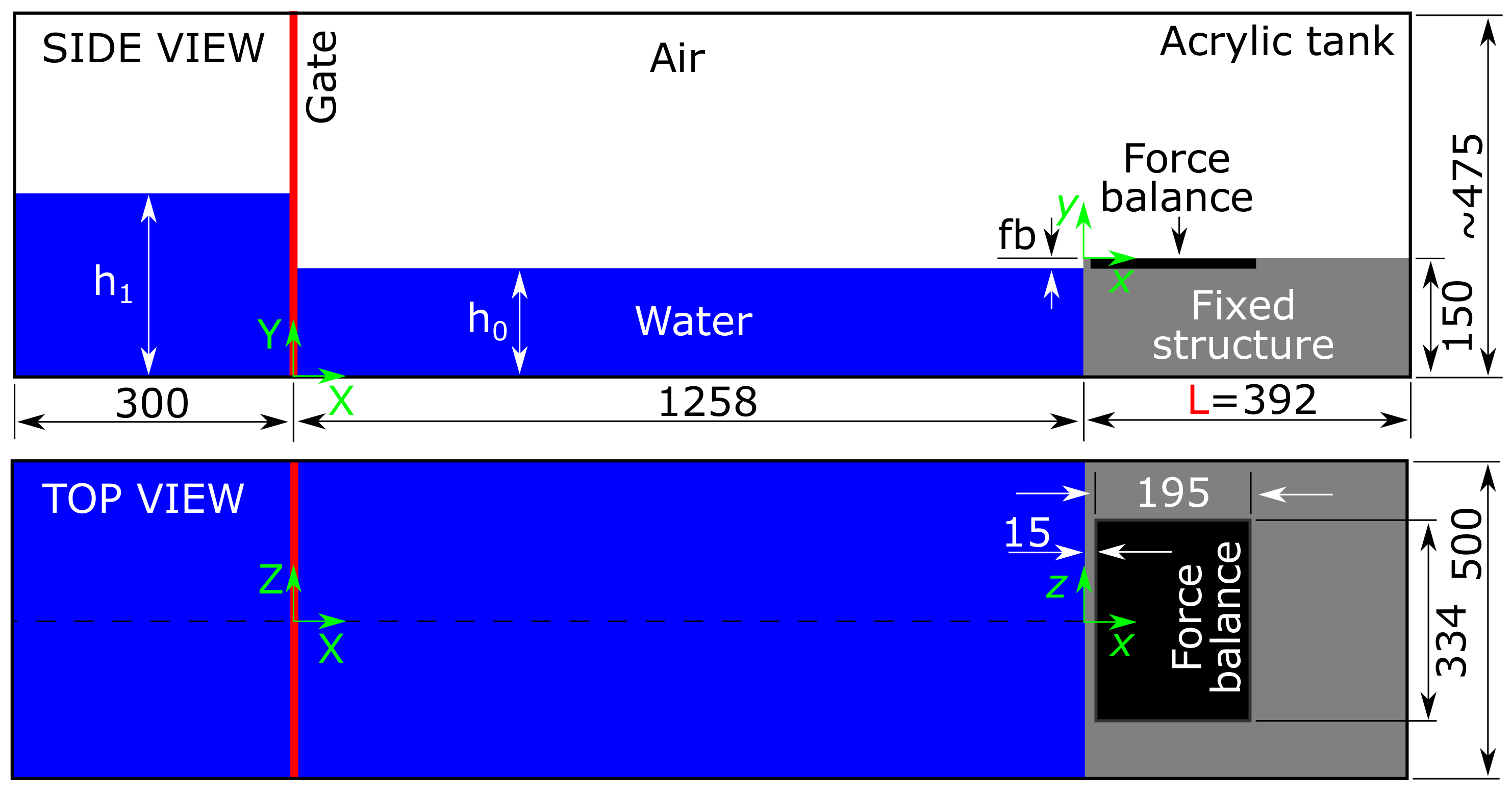
Figure 1 shows the experimental setup. In an acrylic tank of 1.95 m in length, 0.475 m in height and 0.5 m in width, an internal cuboid structure was fixed in a corner, and two water reservoirs separated by a vertical gate. The depths of the lower and higher reservoirs are denoted by and , respectively. When the gate is suddenly removed, the fluid in the upstream reservoir interacts with that located downstream, generating a wet dam-break bore. Subsequently, this bore floods and propagates over the deck of the structure. For the purposes of this work, including the validation and implementation of the model, a study case in which , and (where is the initial freeboard), was considered. This case was chosen because only a negligible cavity was formed in the bore at the start of the deck using these dimensions [14], as is required for this experiment.
Two parameters were considered for the validation of the numerical approach: water elevations and vertical loads. These data are available in open-source repositories provided in [14,57], respectively. The former provides time series of water elevations measured at every centimetre along with the horizontal domain shown in Figure 1. The water elevations were obtained from high-speed videos taken at 500 fps, employing the binary image analysis approach of [58]. The latter provides the time series for vertical loads measured by a force balance embedded in the deck of the fixed structure (see Figure 1). The balance, with a sampling rate of 500 Hz, consists of an arrangement of four S-type load cells supporting a horizontal plate aligned with the deck of the structure. Details of the measuring procedure of the force balance can be found in [14,51,52].
2.2. Numerical Methods
The open-source CFD model OpenFOAM was used to carry out the numerical simulations. OpenFOAM simulates fluid dynamics and continuum mechanics by discretely solving the Navier-Stokes equations. It is supported by the Finite Volume Method (FVM), which works by integrating the partial differential equations to be solved. For this study the system of governing equations contains the mass conservation (Equation (1)), momentum conservation (Equation (2)), and volume fraction equations (Equation (3)):
where ∇ is the nabla operator, U the velocity vector, the fluid density, t the time, the dynamic viscosity, the Reynolds stress tensor, p the pressure, g the gravity acceleration, the surface tension, the surface curvature, a scalar field for the identification of the phases or phase volume fraction, and the relative velocity. Equation (2) is written in terms of the Reynolds stress tensor, (Equation (4)), with being the kinematic turbulent viscosity, the turbulent kinetic energy per unit mass, and I the Kronecker delta.
Equations (1) and (2) are the Reynolds Averaged Navier-Stokes (RANS) equations, which are solved simultaneously for the two immiscible fluids. Turbulence models are introduced to close the Navier-Stokes equations. For example the RANS turbulence models (e.g., Spalart-Allmaras, k-, k-, etc.), which are widely used in industry and engineering.
The numerical simulation of water in a free-surface condition is carried out through Equation (3), which is an advection equation that models the distribution of a scalar field , i.e., for air, for water, the intermediate values represent the fluids’ interface [59].
Within the OpenFOAM framework, interFoam is a multi-phase flow solver for two incompressible, isothermal immiscible fluids. The interface is tracked using a Volume of Fluid (VOF) phase-fraction-based approach, as described by Hirt and Nichols [59]. Previous studies [36,60,61,62,63] have investigated the ability to simulate free-surface with different turbulence models in OpenFOAM.
The roughness modelling was carried out in terms of a sand-grain roughness height () on the deck structure [54,64,65]. The sand-grain roughness height is a theoretical parameter obtained by coating the rough surface with a monolayer of sand grains. However, to facilitate its application on real materials, different authors have related this parameter to measured surface roughness, (e.g., [53,56]). The model calculates the kinematic viscosity of fluid near a wall, , which is obtained as
where is the kinematic viscosity of fluid near the wall, the estimated wall-normal height of the cell centre in wall units (Equation (6)), the von Kármán constant, the modified wall roughness parameter (Equation (7)), and the limited kinematic viscosity near the wall, which is the maximum value between the turbulent viscosity near the wall () and .
where y is the wall-normal height, the empirical model constant, E the wall roughness parameter, the sand-grain roughness height in wall units, and the roughness function parameter (Equation (8)), with being the roughness constant.
2.3. Numerical Setup
Table 1 shows the constant transport properties for the water and air phases in the numerical simulations. The gravity acceleration was given a standard value of . The simulation time was set to and the results were recorded every .
The maximum Courant number was set to and the maximum computation time step to 0.001 s, to ensure the stability of the solution. The Courant number was defined considering the expression , where is the time step and is the cell size in the direction of the velocity U. During the simulations, the mean Courant number remained below 0.0015, and water residuals tend to zero; therefore, the discretized governing equations solution is balanced, and convergence was achieved during the simulation.
The Preconditioned Conjugate Gradient (PCG) solver was selected for the pressure field and a smooth solver for the fluid phases and the velocity fields. The PIMPLE algorithm (i.e., a combination of SIMPLE and PISO algorithms) was used for coupling equations of mass and momentum conservation.
To simulate a free-surface condition, inletOutlet and totalPressure boundary conditions were set at the top of the numerical domain. zeroGradient boundary condition was given for the water field. The velocity field boundary conditions were set as noSlip and with a starting velocity equal to for all the fluid phases, i.e., fluids at rest. The front and back faces, which correspond to the lateral walls of the tank, were set with an empty boundary condition, i.e., a two-dimensional simulation. The turbulent flow field was modelled using the two-equation k- turbulence model, as suggested by [62] for some wet dam-break applications. Since no noticeable deformations were reported during the experiments that motivated this study [14], the deck walls were treated as rigid walls and no fluid-structure interaction analysis was performed.
The deck roughness was simulated with a nutkRoughWallFunction boundary condition, in which the wall roughness parameter is defined. This boundary condition was given for the deck face turbulent viscosity, in . Two parameters were defined when using the nutkRoughWallFunction boundary condition: the roughness height, i.e., sand-grain roughness (e.g., zero for smooth walls), and the roughness constant (e.g., values between 0.5 to 1.0) [66].
2.4. Grid Convergence Study
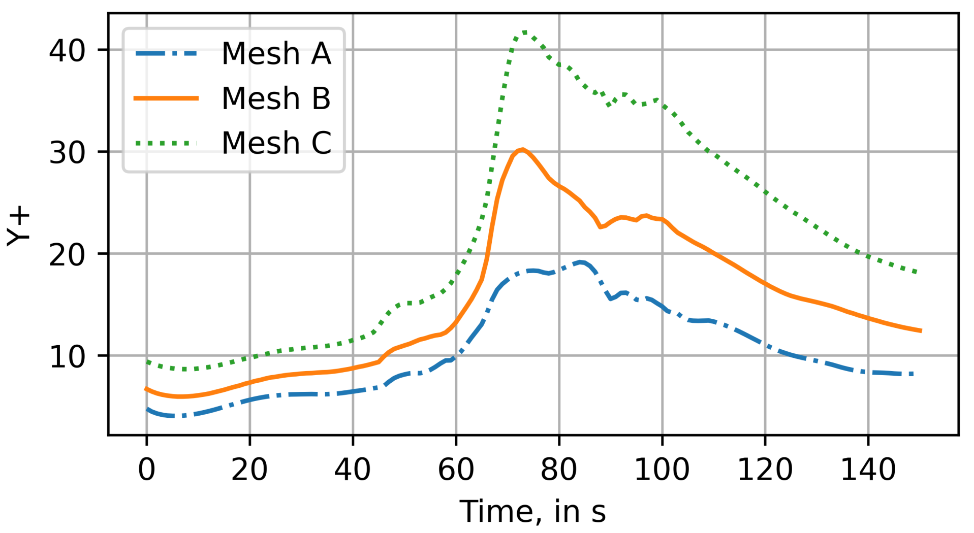
A spatial convergence analysis was performed to determine the discretization errors and the optimal numerical resolution for the simulations. Three mesh configurations with a refinement factor r of [67] were tested. Mesh A, B, and C correspond to fine, medium, and coarse grids, respectively (see Table 2). The mean y+ value for the three mesh configurations is reported in Figure 2.
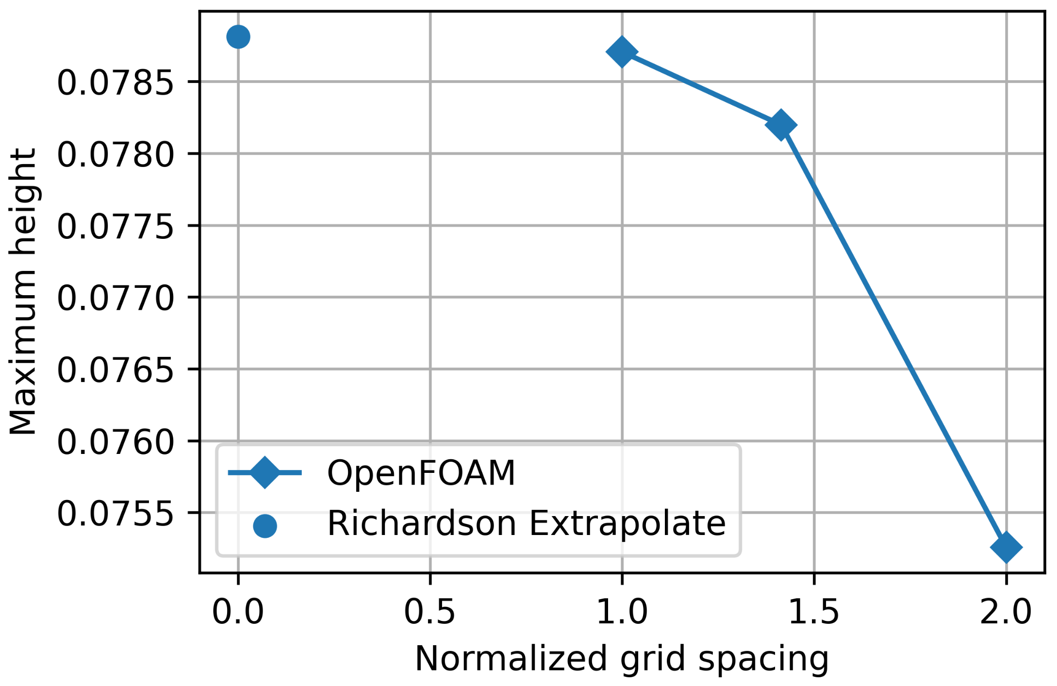
Richardson’s extrapolation method was used to calculate the grid convergence index (GCI) (see [68]). The maximum value for the water surface elevation was measured with a numerical probe located at . The order of convergence was calculated with Equation (9).
Then, an estimate of the value of the maximum surface elevation at zero grid spacing was made, applying Richardson’s extrapolation with the two finest grids (Equation (10)). The GCI for the coarser grid (Mesh B) was calculated with Equation (11), where is the relative error between grids; i.e., and .
Finally, to guarantee that each grid level solution is within the asymptotic range of convergence, must be approximately equal to (). The results of this study are summarized in Figure 3, where the maximum surface elevation for zero grid spacing was with an error band of . Considering the GCI study and the computational time optimization, Mesh B was selected to perform the numerical simulations in this study (see Figure 4 and Table 2 for mesh size).
2.5. Validation of the CFD Results
2.5.1. Free surface Elevation
Experimental results from [57] (i.e., study case and ) were used to perform the validation of the numerical model in OpenFOAM. The free surface elevation was compared for all time instants, considering the time series data taken at , and , all located on the left side of the deck (see Figure 1).
Between experiment and simulation, a phase difference of approximately s was found; to account for this, the simulation was shifted in time s, ranging from . If a time step was not available in both experiment and simulation (due to the time shift or the difference in temporal resolution), the specific time step was omitted and not included in the analysis. Therefore, the number of time steps was reduced to 135.
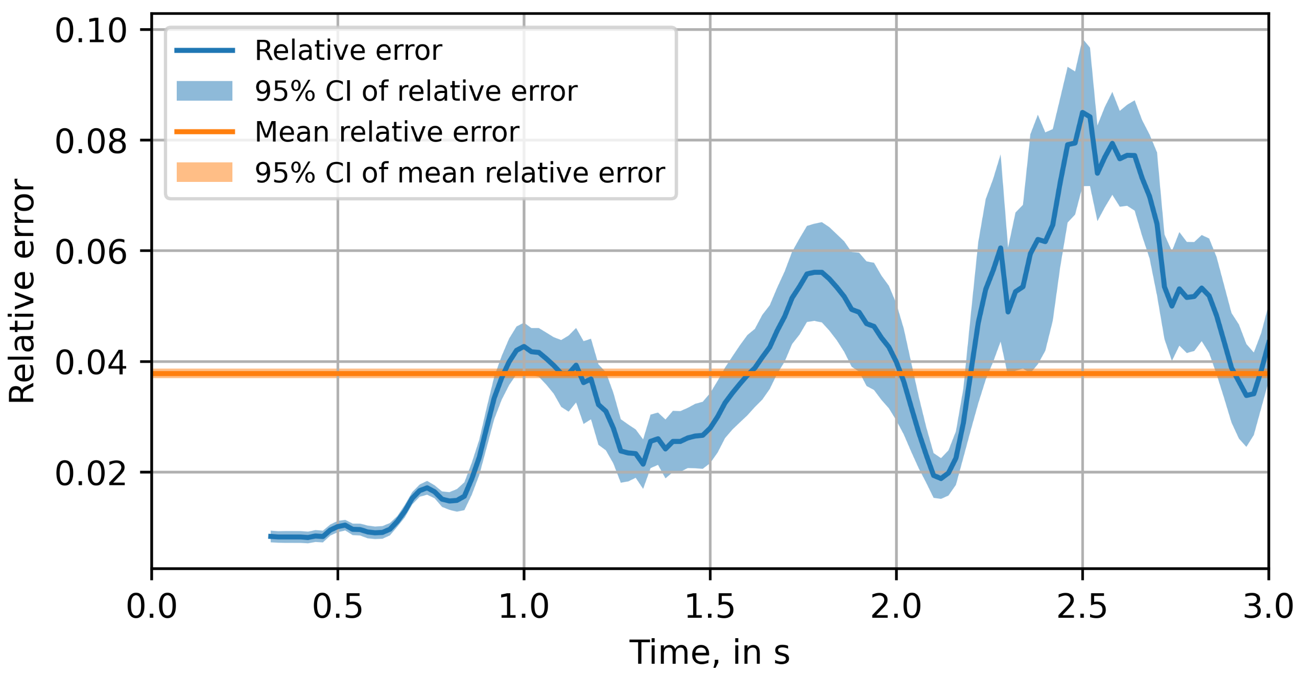
The relative error is given as a function of time, considering all ten probes and the five repetitions of the experiment. Afterwards, the relative error was summarized as the mean relative error E for the entire duration of the experiment, all probes, and all repetitions. The confidence interval (CI) was estimated employing the bootstrap method [69], using the set of all individual relative errors. Thus, the CI of the relative error was based on 50 observations, whereas the CI of the mean relative error was based on 6750 observations. at time step was estimated as
where is the estimator of the relative error in time, the free surface elevation measured in the experiments, the free surface elevation as predicted by the simulation, and and the number of used probes and number of repetitions of the experiment, respectively. The indices denote the time t, probe i and repetition j at which the elevation was measured.
The mean relative error E describes the mean of all available relative errors () and was estimated by
where is the estimator of the mean relative error and the number of time steps used in the analysis.
An estimate of the standard error can be obtained with the bootstrap method [69]. For each error estimation (both, and ), the underlying sample is resampled 500,000 times using a Monte Carlo simulation (drawing randomly from the original sample with replacement). The error for each resample was estimated, resulting in a distribution of errors for the corresponding estimator of the error. Assuming a normal distribution, a 95 % CI was calculated by and , respectively. The estimator of the mean relative error was calculated as , with an estimated standard error/deviation of with a 95% CI ranging from 3.696% to 3.871% (Figure 5).
2.5.2. Vertical Loads
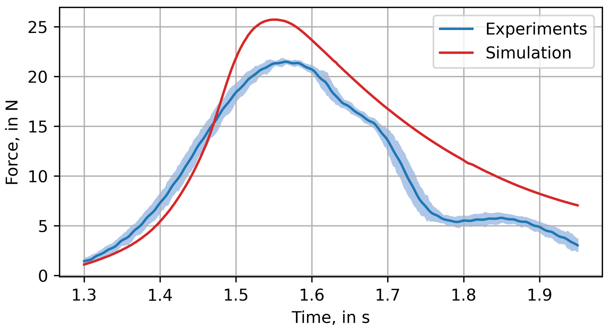
The vertical loads on the deck structure were compared against the experimental results of [14]. The vertical load exerted on the surface was evaluated over the length of m (2D-simulation), starting from the x-position m. Figure 6 shows the vertical load curves of both experimental data and numerical simulations with OpenFOAM. As suggested in [14], a parameter was defined as the ratio of the areas under the curve of the experimental and numerical results in a time interval of s. This parameter accounts for the overestimation of the global loading in the deck structure. In this case, the parameter suggests that the total load obtained with the numerical model overestimates the experiments about 1.25 times (); however, it captures the trend of the experimental results, ascertaining quite well the time at which the peak values occurred (Figure 6). The mean absolute error was calculated as 3.39 N, with a standard deviation of 0.048 N and 95% CI. As shown in [41], the differences in vertical loads by a similar force balance in numerical and experimental results can be associated with the velocity of the gate, which was considered as instantaneous in this work.
2.6. Study Cases
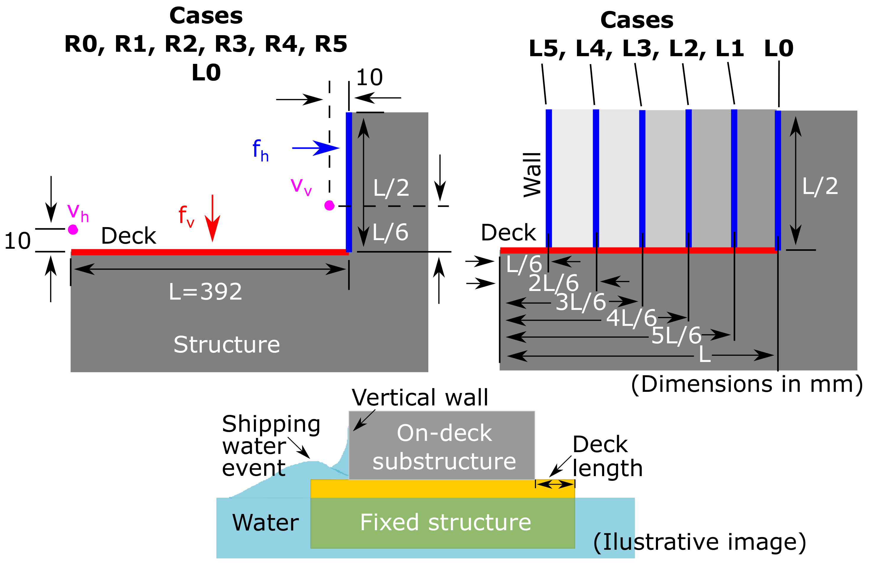
Twelve study cases were simulated to separately evaluate the effect of the variation of the deck roughness and the deck length on some shipping water parameters: punctual horizontal flow velocity at the deck edge (), punctual vertical flow velocity close to the deck wall (), vertical load over the complete deck () and horizontal load over the complete deck wall (), as defined in Figure 7. For all cases, the same incident flow was considered (i.e., a wet dam-break bore generated with and ).
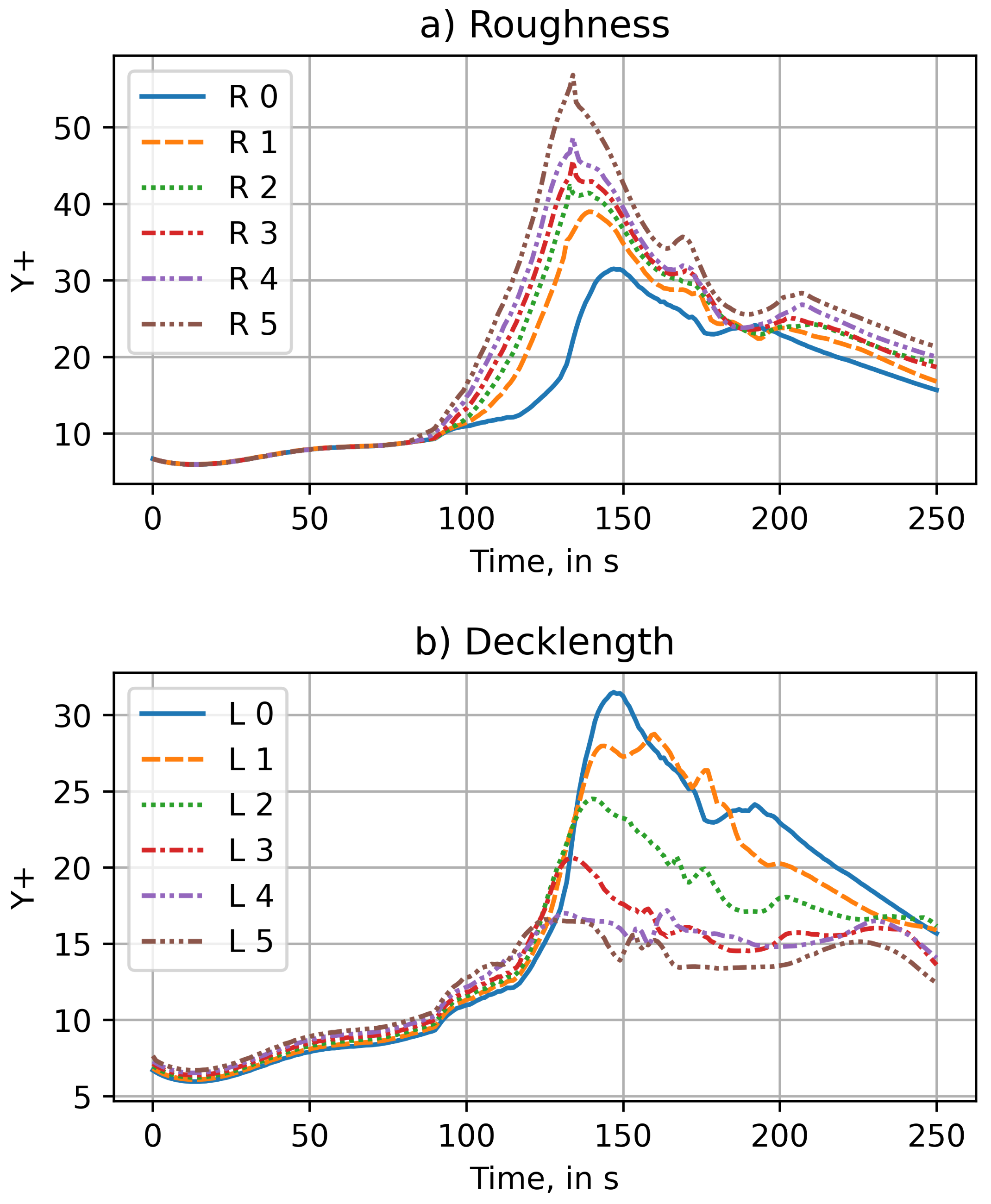
Table 3 and Figure 7 show the study cases used to investigate the effect of deck roughness (R0-R5) and deck length (L0-L5). The table shows the equivalent sand-grain roughness , in , for the selected study cases R0-R5, in which the deck length was kept constant (L = 0.392). For the cases L0-L5, the total length of the numerical domain was preserved and the deck length was reduced consecutively by (i.e., L/6), disregarding deck roughness (see Figure 7). Figure 8 shows the mean y+ value for the twelve study cases, which remains within the range of application when using wall functions to capture the near wall velocity profile [70].
3. Results and Discussion
3.1. The Effect of Deck Roughness
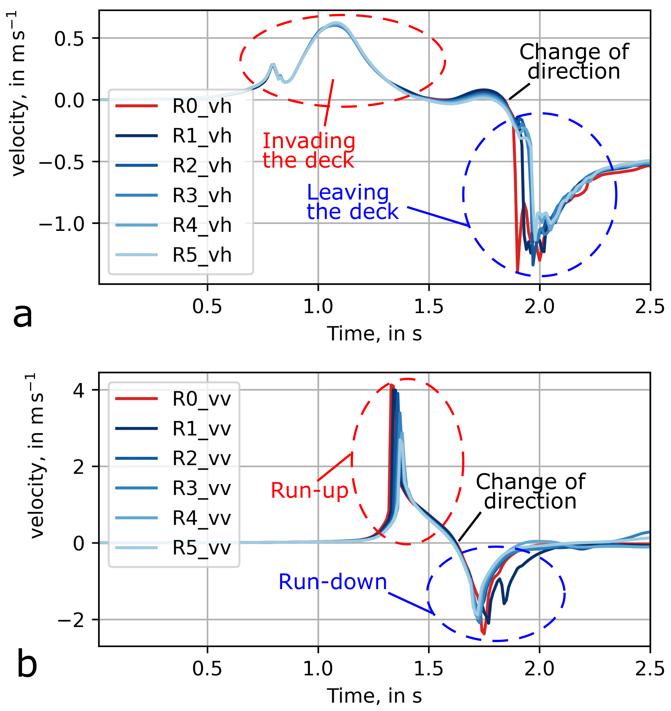
Figure 9 shows the effect of different deck roughnesses on the horizontal and vertical flow velocities, which were measured punctually at the positions shown in Figure 7 ( and , respectively). Although these parameters may present spatio-temporal variations during the shipping water events [13,24], the data reported here gives an idea about the velocity at which the water invades the deck and interacts with the on-deck wall. For instance, knowing the horizontal velocity of the water is relevant for the implementation of models to represent the water elevations over the deck [9,19].
Figure 9a presents the comparison of horizontal flow velocities () for different roughnesses (cases R0–R5). The positive velocities correspond to the stage in which the shipping water event invades the deck, whereas the negative values correspond to the backflow stage when the shipped flow returns to the reservoir. As expected, the deck roughness did not affect the velocity at the deck edge (see first peak values, ∼0.6 m/s). However, it did influence the backflow velocities (see minimum values in ). A small reduction in maximum values with respect to the reference case (R0) was observed as the roughness increased. Furthermore, there was a short delay in the occurrence of these maximum values.
For the case of (Figure 9b), two stages can be identified, run-up (positive velocity values) and run-down (negative values), whose peaks can be identified at and , respectively. Results suggest that there is a decrease in peak vertical velocities for each case, as roughness increases. The maximum roughness (R5) decreased the maximum during the run-up in ∼35%, with respect to the reference case (R0), whereas a reduction of ∼5% was seen during run-down.
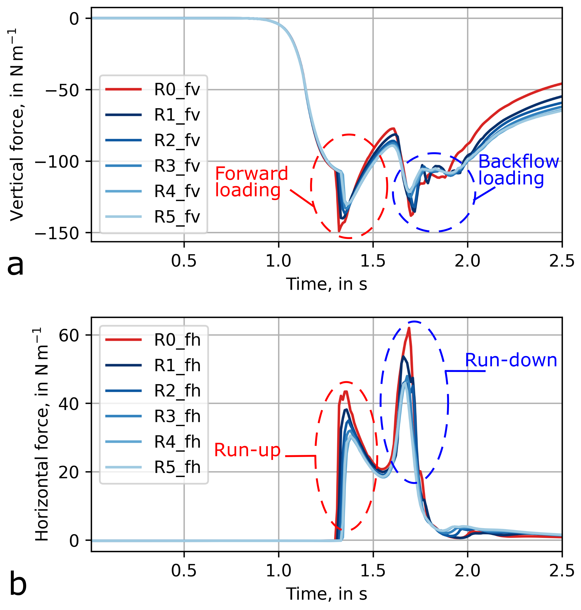
The effect of deck roughness on the shipping water loads is seen in Figure 10. The vertical loads () are shown in Figure 10a. Note that the negative values indicate the downward direction of the loads. Two peak values can be observed at 1.3 s and 1.7 s. These correspond to the stages of forward and backflow vertical loading, respectively, as defined by [51] in experimental observations. As shown in that work, these stages are found in shipping water events that have an obstruction, such as a vertical wall on the deck. The forward loads occur from the start of the deck to the final stage of run-up on the wall, whereas the backflow vertical loading includes the run-down on the wall and the flow returning to the reservoir. Note that as roughness increases, the peak vertical loads tend to decrease in these stages. For the highest roughness (case R5), this decrease is ∼10% when compared to the reference case (R0). This behaviour is also observed for the horizontal loads generated on the vertical wall (, Figure 10b), whose time series present two peak values, corresponding to the maximum loads in the run-up and run-down stages. Considering the maximum values of the case with the greatest roughness (R6), this peak amplitude reduction was between 20–25% when compared to the R0 case.
Results suggest that the deck roughness reduces the peak values of shipping water loads, although the trends of the time series are similar. Even though the initial conditions (i.e., incident wave) remain constant for all the study cases, as roughness increases the flow velocity decreases, which seems to cause a reduction in the dynamic component of the force, as reflected in the reduction and delay in load peak values.
In this study, a shipping water scenario was chosen in which the layer of water over the deck was significant (see snapshots in case study 3 in [14]). Perhaps, in the analysis of shipping water scenarios with a smaller water layer over the deck (e.g., Case study 1 in [57]), the effect of roughness on the flow propagation may be more considerable.
The present evaluations consider theoretical deck roughness. Further research should be carried out to relate these results to real applications, including decks of structures with texture or structural arrangements over them. Examples include decks with vegetation, pipeline arrangements, arrangement of structural panels, sand, rocks, corroded surfaces, fouling, arrangements of substructures or equipment, or other elements distributed on the deck that, for practical purposes, could be considered in terms of roughness parameters.
3.2. The Effect of Deck Length
The effect of deck length in shipping water loads could differ depending of the structure configuration. For instance, the loading trends may differ if there is, or is not, an obstruction in the way of the shipping water flow, such as a vertical wall. The shipping water can occur on the bow, stern, or sides of ships [41], typically with significant differences in the length of the corresponding side-deck. Therefore, the loading trends may have different behaviour, depending on the location of shipping. Hernández-Fontes et al. [51] compared experimental vertical loads for two different deck lengths, showing that the backflow loads may show a significant peak for the shortest length. This peak could have relevance in the structural behaviour of fixed structures or the dynamics of floating ones. To strengthen this knowledge, in this study several deck lengths (Figure 7) are considered.
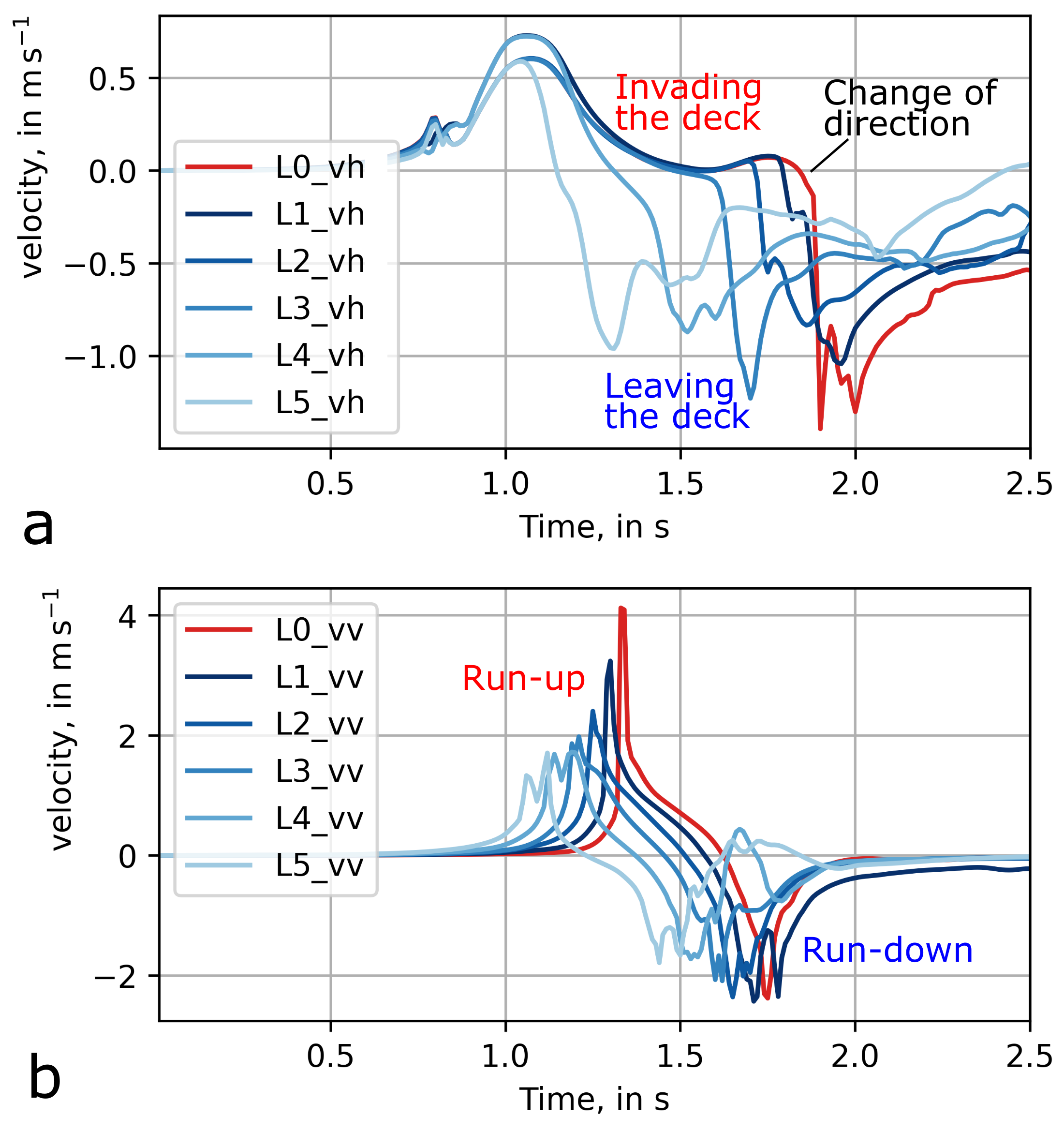
The effect of deck length on the shipping water velocities and is shown in Figure 11a,b, respectively. For , note that during the invasion of water over the deck and water leaving the deck(returning to the reservoir), the maximum velocities were in the order of 0.5–0.7 m/s and 0.9–1.4 m/s, respectively. For most cases, as the deck length increases, the maximum backflow velocity did also, and, as expected, the reduction of the deck length brought backward its occurrence. For the case of , it is observed that the increase in deck length is related to the increase in the maximum run-up and run-down velocities. During run-up, the shorter decks brought backward the occurrence of the maximum velocities compared to the longest deck (case L0).
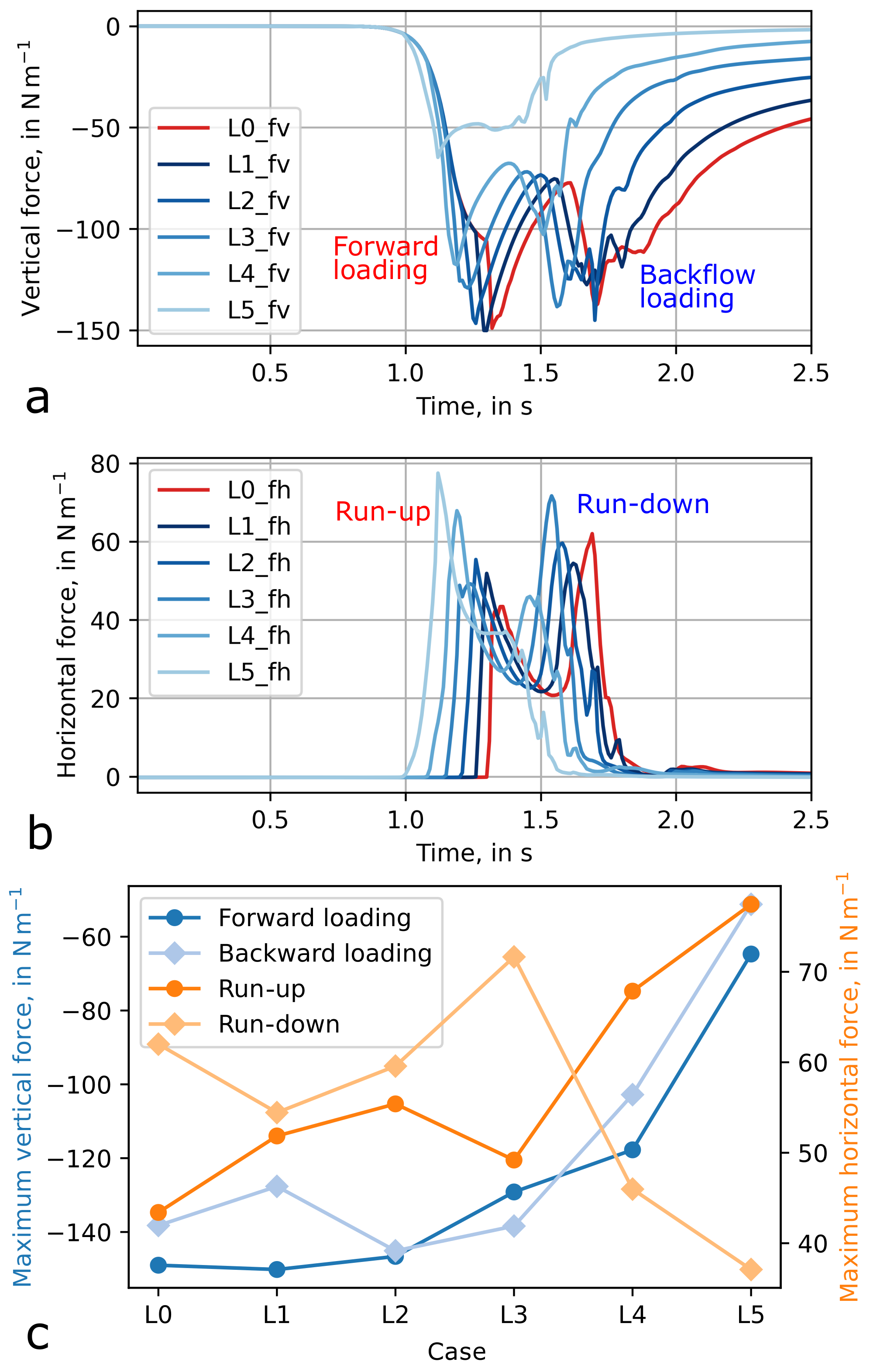
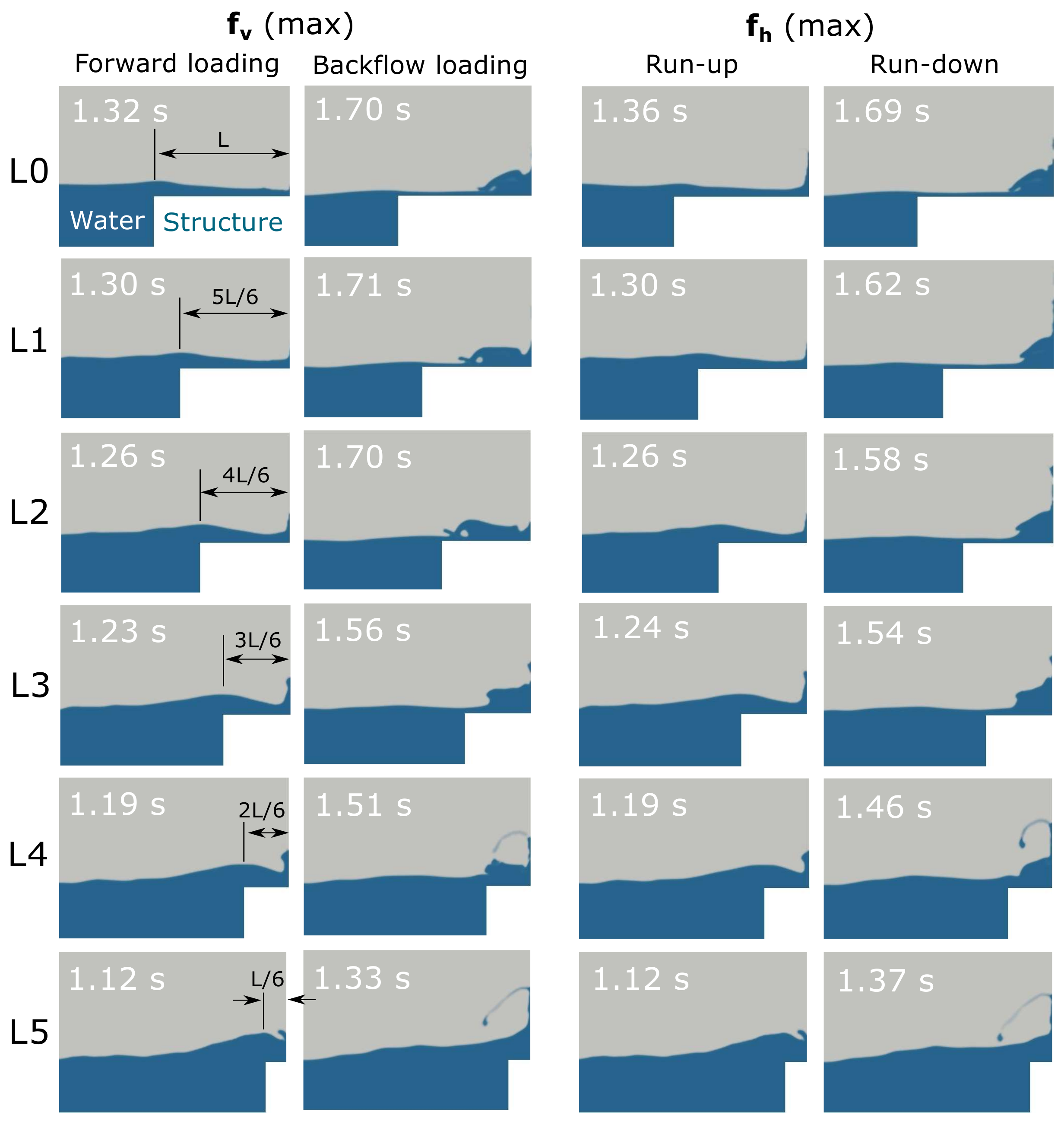
Figure 12 presents the effect of deck length on shipping water loads, whereas Figure 13 illustrates some snapshots taken at the stages when the maximum loads occurred.
Figure 12a shows the effect of deck length on the vertical loads on the deck (). Two peak loads related to the forward and backflow loading are presented in all cases. Moreover, the deck length and the time of occurrence of the peaks are directly correlated. For most cases, the order of magnitude of the maximum backflow loads is as significant as for the maximum forward flow loads.
Concerning the horizontal loads (, Figure 12b), all the cases showed two peaks during the run-up and run-down stages. Note that as the deck length is reduced, the horizontal loads tend to increase during run-up, occurring earlier than for longer decks. This trend can be seen in Figure 12c, which shows the tendency of maximum vertical and horizontal loads for the different cases.
These results are interesting from the point of view of structural design. It has been demonstrated that there are two triggering stages (see peak loads) during a shipping water event in a deck with finite length restricted by a vertical wall. For the vertical loads, these peaks are observed during the forward and backflow loading stages, whereas for the horizontal loads exerted on a vertical wall, these are found during the run-up and run-down. The maximum loads during these stages may be of a similar order of magnitude in some cases; therefore, this should be considered in the design of fixed or floating structures.
4. Conclusions
A systematic numerical investigation was performed to obtain an initial understanding of the effect of deck roughness and deck length on the kinematics and loads of shipping water. We considered the case of an isolated shipping water event generated with the wet dam-break approach. This practical method allowed systematic analyses of rapid wave-deck interactions to be carried out, varying the roughness and length of the deck.
From the results, it can be seen that an increase in deck roughness minimizes the maximum flow velocities and loads, and delays their occurrence. Despite the general load trends are maintained, it tends to reduce the maximum vertical and horizontal loads observed during the forward and backflow stages. It is worth noting that in this work, the shipping water event considered as reference did not have a significant air cavity at the bow edge, although a significant water volume was generated on the deck. Thus, the effect of roughness in flow propagation could be seen more easily in the cases with less water on the deck. The approach presented could be used to evaluate the effect of roughness on different types of shipping water. Further work could also be done to relate the theoretical roughness values considered in numerical simulations to real applications, including validation with experimental data of the roughness approach in OpenFoam.
The deck length also affects shipping water kinematics and loads as follows: shorter decks lead to the earlier occurrence of maximum velocities and tend to increase the horizontal loads on the vertical wall during the run-up. In cases where shipping water propagates over decks of finite length (i.e., with a vertical wall downstream), two impulsive load events can be identified, related to the forward and backflow loading stages. These should be considered for the design of fixed or floating structures subjected to shipping water events.
Author Contributions
Conceptualization, J.V.H.F., M.R. and P.E.R.-O.; methodology, J.V.H.F., M.R. and P.E.R.-O.; software, M.R. and P.E.R.-O.; validation, M.R. and P.E.R.-O.; formal analysis, J.V.H.F.; investigation, J.V.H.F.; resources, J.V.H.F., M.R. and P.E.R.-O.; data curation, J.V.H.F., M.R., E.M., R.S. and P.E.R.-O.; writing—original draft preparation, J.V.H.F., M.R., and P.E.R.-O.; writing—review and editing, J.V.H.F., M.R., P.E.R.-O., R.S. and E.M.; visualization, J.V.H.F., M.R. and P.E.R.-O.; supervision, R.S. and E.M.; project administration, R.S. and E.M.; funding acquisition, R.S. All authors have read and agreed to the published version of the manuscript.
Funding
This research was funded by the CONACYT-SENER-SUSTENTABILIDAD ENERGÉTICA project: FSE-2014-06-249795 “Centro Mexicano de Innovación en Energía del Océano (CEMIE Océano)”.
Institutional Review Board Statement
Not applicable.
Informed Consent Statement
Not applicable.
Data Availability Statement
Not applicable.
Acknowledgments
The help provided by Jill Taylor in the revision of the manuscript is gratefully acknowledged. J.V.H.F. thanks the support provided by “Gratificação de Produtividade Acadêmica (GPA) da Universidade do Estado do Amazonas, Portaria Nº 086/2021-GR/UEA”.
Conflicts of Interest
The authors declare no conflict of interest. The funders had no role in the design of the study; in the collection, analyses, or interpretation of data; in the writing of the manuscript, or in the decision to publish the results.
Abbreviations
The following abbreviations are used in this manuscript:
| FPSO | Floating production, storage and offloading |
| CFD | Computational fluid dynamics |
| CI | Confidence interval |
| FVM | Finite volume method |
| RANS | Reynolds averaged Navier-Stokes |
| GCI | Grid convergence index |
| PCG | Preconditioned conjugate gradient |
| SIMPLE | semi-implicit method for pressure-linked equations |
| PISO | pressure-implicit split-operator |
References
- Greco, M. A Two-Dimensional Study of Green-Water Loading. Ph.D. Thesis, Norwegian University of Science and Technology, Trondheim, Norway, 2001. [Google Scholar]
- Buchner, B. Green Water on Ship-Type Offshore Structures. Ph.D. Thesis, Delft University of Technology, Delft, The Netherland, 2002. [Google Scholar]
- Rajendran, S.; Fonseca, N.; Soares, C.G. Body nonlinear time domain calculation of vertical ship responses in extreme seas accounting for 2nd order Froude-Krylov pressure. Appl. Ocean Res. 2016, 54, 39–52. [Google Scholar] [CrossRef]
- Van Essen, S.M.; Monroy, C.; Shen, Z.; Helder, J.; Kim, D.H.; Seng, S.; Ge, Z. Screening wave conditions for the occurrence of green water events on sailing ships. Ocean Eng. 2021, 234, 109218. [Google Scholar] [CrossRef]
- Zhu, R.; Miao, G.; Lin, Z. Numerical research on FPSOs with green water occurrence. J. Ship Res. 2009, 53, 7–18. [Google Scholar] [CrossRef]
- Greco, M.; Landrini, M.; Faltinsen, O. Impact flows and loads on ship-deck structures. J. Fluids Struct. 2004, 19, 251–275. [Google Scholar] [CrossRef]
- Goda, K.; Miyamoto, T. A study of shipping water pressure on deck by two-dimensional ship model tests. J. Soc. Nav. Archit. Jpn. 1976, 1976, 16–22. [Google Scholar] [CrossRef]
- Ogawa, Y.; Taguchi, H.; Ishida, S. Experimental study on shipping water volume and its load on deck. J. Soc. Nav. Archit. Jpn. 1997, 1997, 177–185. [Google Scholar] [CrossRef]
- Hernández-Fontes, J.V.; Vitola, M.A.; de Tarso, T.E.P.; Sphaier, S.H. Analytical convolution model for shipping water evolution on a fixed structure. Appl. Ocean Res. 2019, 82, 415–429. [Google Scholar] [CrossRef]
- Hu, Z.; Xue, H.; Tang, W.; Zhang, X. A combined wave-dam-breaking model for rogue wave overtopping. Ocean Eng. 2015, 104, 77–88. [Google Scholar] [CrossRef]
- Zhang, X.; Draper, S.; Wolgamot, H.; Zhao, W.; Cheng, L. Eliciting features of 2D greenwater overtopping of a fixed box using modified dam break models. Appl. Ocean Res. 2019, 84, 74–91. [Google Scholar] [CrossRef]
- Zhang, X.; Tian, X.; Guo, X.; Li, X.; Xiao, L. Bottom step enlarging horizontal momentum flux of dam break flow. Ocean Eng. 2020, 214, 107729. [Google Scholar] [CrossRef]
- Ryu, Y.; Chang, K.A.; Mercier, R. Application of dam-break flow to green water prediction. Appl. Ocean Res. 2007, 29, 128–136. [Google Scholar] [CrossRef]
- Hernández-Fontes, J.V.; Vitola, M.A.; Esperança, P.T.T.; Sphaier, S.H. Assessing shipping water vertical loads on a fixed structure by convolution model and wet dam-break tests. Appl. Ocean Res. 2018, 82, 63–73. [Google Scholar] [CrossRef]
- Fontes, J.V.H.; Hernández, I.D.; Mendoza, E.; Silva, R.; Silva, E.B.; Sousa, M.R.; Gonzaga, J.; Kamezaki, R.S.F.; Torres, L.; Esperança, P.T.T. On the evolution of different types of green water events. Water 2021, 19, 1148. [Google Scholar] [CrossRef]
- Greco, M.; Colicchio, G.; Faltinsen, O. Shipping of water on a two-dimensional structure. Part 2. J. Fluid Mech. 2007, 581, 371. [Google Scholar] [CrossRef]
- Yan, B.; Luo, M.; Bai, W. An experimental and numerical study of plunging wave impact on a box-shape structure. Mar. Struct. 2019, 66, 272–287. [Google Scholar] [CrossRef]
- Lee, H.H.; Lim, H.J.; Rhee, S.H. Experimental investigation of green water on deck for a CFD validation database. Ocean Eng. 2012, 42, 47–60. [Google Scholar] [CrossRef]
- Hernández-Fontes, J.V.; Hernández, I.D.; Mendoza, E.; Silva, R. Green water evolution on a fixed structure induced by incoming wave trains. Mech. Based Des. Struct. Mach. 2020, 1–29. [Google Scholar] [CrossRef]
- Hernández-Fontes, J.V.; Vitola, M.A.; Silva, M.C.; Esperança, P.D.T.T.; Sphaier, S.H. Use of wet dam-break to study green water problem. In Proceedings of the International Conference on Offshore Mechanics and Arctic Engineering, Ocean Engineering, Trondheim, Norway, 25–30 June 2017; American Society of Mechanical Engineers: New York, NY, USA, 2017; Volume 7A, p. V07AT06A065. [Google Scholar]
- Hernández-Fontes, J.V.; Mendoza, E.; Hernández, I.D.; Silva, R. A detailed description of flow-deck interaction in consecutive green water events. J. Offshore Mech. Arct. Eng. 2021, 143, 041203. [Google Scholar] [CrossRef]
- Silva, D.F.; Coutinho, A.L.; Esperança, P.T. Green water loads on FPSOs exposed to beam and quartering seas, part I: Experimental tests. Ocean Eng. 2017, 140, 419–433. [Google Scholar] [CrossRef]
- Gómez-Gesteira, M.; Cerqueiro, D.; Crespo, C.; Dalrymple, R. Green water overtopping analyzed with a SPH model. Ocean Eng. 2005, 32, 223–238. [Google Scholar] [CrossRef]
- Song, Y.K.; Chang, K.A.; Ariyarathne, K.; Mercier, R. Surface velocity and impact pressure of green water flow on a fixed model structure in a large wave basin. Ocean Eng. 2015, 104, 40–51. [Google Scholar] [CrossRef]
- Mendez, V.; Di Giuseppe, M.; Pasta, S. Comparison of hemodynamic and structural indices of ascending thoracic aortic aneurysm as predicted by 2-way FSI, CFD rigid wall simulation and patient-specific displacement-based FEA. Comput. Biol. Med. 2018, 100, 221–229. [Google Scholar] [CrossRef] [PubMed]
- Rinaudo, A.; Raffa, G.M.; Scardulla, F.; Pilato, M.; Scardulla, C.; Pasta, S. Biomechanical implications of excessive endograft protrusion into the aortic arch after thoracic endovascular repair. Comput. Biol. Med. 2015, 66, 235–241. [Google Scholar] [CrossRef]
- Spalart, P.; Venkatakrishnan, V. On the role and challenges of CFD in the aerospace industry. Aeronaut. J. 2016, 120, 209–232. [Google Scholar] [CrossRef] [Green Version]
- Ding, H.; Visser, F.; Jiang, Y.; Furmanczyk, M. Demonstration and validation of a 3D CFD simulation tool predicting pump performance and cavitation for industrial applications. J. Fluids Eng. 2011, 133, 011101. [Google Scholar] [CrossRef]
- Mohammadian, A.; Kheirkhah Gildeh, H.; Nistor, I. CFD modeling of effluent discharges: A review of past numerical studies. Water 2020, 12, 856. [Google Scholar] [CrossRef] [Green Version]
- Silva, D.F.; Esperança, P.T.; Coutinho, A.L. Green water loads on FPSOs exposed to beam and quartering seas, Part II: CFD simulations. Ocean Eng. 2017, 140, 434–452. [Google Scholar] [CrossRef]
- Greco, M.; Faltinsen, O.; Landrini, M. Shipping of water on a two-dimensional structure. J. Fluid Mech. 2005, 525, 309. [Google Scholar] [CrossRef]
- Greco, M.; Lugni, C. 3-D seakeeping analysis with water on deck and slamming. Part 1: Numerical solver. J. Fluids Struct. 2012, 33, 127–147. [Google Scholar] [CrossRef]
- Greco, M.; Bouscasse, B.; Lugni, C. 3-D seakeeping analysis with water on deck and slamming. Part 2: Experiments and physical investigation. J. Fluids Struct. 2012, 33, 148–179. [Google Scholar] [CrossRef]
- Pham, X.; Varyani, K. Evaluation of green water loads on high-speed containership using CFD. Ocean Eng. 2005, 32, 571–585. [Google Scholar] [CrossRef]
- Östman, A.; Pakozdi, C.; Sileo, L.; Stansberg, C.T.; de Carvalho e Silva, D.F. A fully nonlinear RANS-VOF numerical wavetank applied in the analysis of green water on FPSO in waves. In Proceedings of the International Conference on Offshore Mechanics and Arctic Engineering, San Francisco, CA, USA, 8–13 June 2014; American Society of Mechanical Engineers: New York, NY, USA, 2014; Volume 45516, p. V08BT06A010. [Google Scholar]
- Khojasteh, D.; Tavakoli, S.; Dashtimanesh, A.; Dolatshah, A.; Huang, L.; Glamore, W.; Sadat-Noori, M.; Iglesias, G. Numerical analysis of shipping water impacting a step structure. Ocean Eng. 2020, 209, 107517. [Google Scholar] [CrossRef]
- Pal, S.K.; Kudupudi, R.B.; Sunny, M.R.; Datta, R. Numerical investigation of green water loading on flexible structures using three-step CFD-BEM-FEM approach. J. Mar. Sci. Appl. 2018, 17, 432–442. [Google Scholar] [CrossRef]
- Chen, L.; Taylor, P.H.; Draper, S.; Wolgamot, H. 3-D numerical modelling of greenwater loading on fixed ship-shaped FPSOs. J. Fluids Struct. 2019, 84, 283–301. [Google Scholar] [CrossRef]
- Le Touzé, D.; Marsh, A.; Oger, G.; Guilcher, P.; Khaddaj-Mallat, C.; Alessandrini, B.; Ferrant, P. SPH simulation of green water and ship flooding scenarios. J. Hydrodyn. 2010, 22, 231–236. [Google Scholar] [CrossRef]
- Sanchez-Mondragon, J.; Hernández-Fontes, J.; Vázquez-Hernández, A.; Esperança, P. Wet dam-break simulation using the SPS-LES turbulent contribution on the WCMPS method to evaluate green water events. Comput. Part. Mech. 2019, 7, 705–724. [Google Scholar] [CrossRef]
- Areu-Rangel, O.S.; Hernández-Fontes, J.V.; Silva, R.; Esperança, P.T.; Klapp, J. Green water loads using the wet dam-break method and SPH. Ocean Eng. 2021, 219, 108392. [Google Scholar] [CrossRef]
- Bašić, J.; Degiuli, N.; Malenica, Š.; Ban, D. Lagrangian finite-difference method for predicting green water loadings. Ocean Eng. 2020, 209, 107533. [Google Scholar] [CrossRef]
- Shao, S.; Ji, C.; Graham, D.I.; Reeve, D.E.; James, P.W.; Chadwick, A.J. Simulation of wave overtopping by an incompressible SPH model. Coastal Eng. 2006, 53, 723–735. [Google Scholar] [CrossRef]
- Yan, B.; Bai, W.; Qian, L.; Ma, Z. Study on hydro-kinematic characteristics of green water over different fixed decks using immersed boundary method. Ocean Eng. 2018, 164, 74–86. [Google Scholar] [CrossRef]
- Lee, G.N.; Jung, K.H.; Chae, Y.J.; Park, I.R.; Malenica, S.; Chung, Y.S. Experimental and numerical study of the behaviour and flow kinematics of the formation of green water on a rectangular structure. Brodogr. Teor. Praksa Brodogr. Pomor. Teh. 2016, 67, 133–145. [Google Scholar] [CrossRef] [Green Version]
- Hernández-Fontes, J.V.; Vitola, M.A.; Silva, M.C.; Esperança, P.D.T.T.; Sphaier, S.H. On the generation of isolated green water events using wet dam-break. J. Offshore Mech. Arct. Eng. 2018, 140, 051101. [Google Scholar] [CrossRef]
- Niklas, K.; Pruszko, H. Full-scale CFD simulations for the determination of ship resistance as a rational, alternative method to towing tank experiments. Ocean Eng. 2019, 190, 106435. [Google Scholar] [CrossRef]
- Asnaghi, A.; Svennberg, U.; Gustafsson, R.; Bensow, R.E. Propeller tip vortex mitigation by roughness application. Appl. Ocean Res. 2021, 106, 102449. [Google Scholar] [CrossRef]
- Shibata, K.; Koshizuka, S. Numerical analysis of shipping water impact on a deck using a particle method. Ocean Eng. 2007, 34, 585–593. [Google Scholar] [CrossRef]
- Lee, G.N.; Jung, K.H.; Malenica, S.; Chung, Y.S.; Suh, S.B.; Kim, M.S.; Choi, Y.H. Experimental study on flow kinematics and pressure distribution of green water on a rectangular structure. Ocean Eng. 2020, 195, 106649. [Google Scholar] [CrossRef]
- Hernández-Fontes, J.V.; Vitola, M.A.; Esperança, P.T.T.; Sphaier, S.H.; Silva, R. Patterns and vertical loads in water shipping in systematic wet dam-break experiments. Ocean Eng. 2020, 197, 106891. [Google Scholar] [CrossRef]
- Hernández-Fontes, J.V.; Esperança, P.T.; Silva, R.; Mendoza, E.; Sphaier, S.H. Violent water-structure interaction: Overtopping features and vertical loads on a fixed structure due to broken incident flows. Mar. Struct. 2020, 74, 102816. [Google Scholar] [CrossRef]
- Adams, T.; Grant, C.; Watson, H. A Simple Algorithm to Relate Measured Surface Roughness to Equivalent Sand-grain Roughness. Int. J. Mech. Eng. Mechatron. 2012, 1, 66–71. [Google Scholar] [CrossRef]
- Speranza, N.; Kidd, B.; Schultz, M.P.; Viola, I.M. Modelling of hull roughness. Ocean Eng. 2019, 174, 31–42. [Google Scholar] [CrossRef] [Green Version]
- Bhatt, C.P.; McClain, S.T. Assessment of uncertainty in equivalent sand-grain roughness methods. ASME Int. Mech. Eng. Congr. Expo. Proc. 2008, 8 Pt A, 719–728. [Google Scholar] [CrossRef] [Green Version]
- Lee, S.; Hwang, W.; Yee, K. Robust design optimization of a turbine blade film cooling hole affected by roughness and blockage. Int. J. Therm. Sci. 2018, 133, 216–229. [Google Scholar] [CrossRef]
- Hernández-Fontes, J.V.; Esperança, P.T.T.; Graniel, J.F.B.; Sphaier, S.H.; Silva, R. Green Water on A Fixed Structure Due to Incident Bores: Guidelines and Database for Model Validations Regarding Flow Evolution. Water 2019, 11, 2584. [Google Scholar] [CrossRef] [Green Version]
- Hernández, I.D.; Hernández-Fontes, J.V.; Vitola, M.A.; Silva, M.C.; Esperança, P.T. Water elevation measurements using binary image analysis for 2D hydrodynamic experiments. Ocean Eng. 2018, 157, 325–338. [Google Scholar] [CrossRef]
- Hirt, C.W.; Nichols, B.D. Volume of fluid (VOF) method for the dynamics of free boundaries. J. Comput. Phys. 1981, 39, 201–225. [Google Scholar] [CrossRef]
- Lopes, P. Free-Surface Flow Interface and Air-Entrainment Modelling Using OpenFOAM. Ph.D. Thesis, University of Coimbra, Coimbra, Portugal, 2013. [Google Scholar]
- Gatin, I.; Cvijetić, G.; Vukčević, V.; Jasak, H.; Malenica, Š. Harmonic Balance method for nonlinear and viscous free surface flows. Ocean Eng. 2018, 157, 164–179. [Google Scholar] [CrossRef]
- Rodríguez-Ocampo, P.E.; Ring, M.; Hernández-Fontes, J.V.; Alcérreca-Huerta, J.C.; Mendoza, E.; Silva, R. CFD Simulations of Multiphase Flows: Interaction of Miscible Liquids with Different Temperatures. Water 2020, 12, 2581. [Google Scholar] [CrossRef]
- Rodríguez-Ocampo, P.E.; Ring, M.; Hernández-Fontes, J.V.; Alcérreca-Huerta, J.C.; Mendoza, E.; Gallegos-Diez-Barroso, G.; Silva, R. A 2D Image-Based Approach for CFD Validation of Liquid Mixing in a Free-Surface Condition. J. Appl. Fluid Mech. 2020, 13, 1487–1500. [Google Scholar] [CrossRef]
- OPENFOAM®. OpenFOAM: User Guide v2006; The OpenFOAM Foundation Ltd.: London, UK, 2006. [Google Scholar]
- Knopp, T.; Eisfeld, B.; Calvo, J.B. A new extension for k-ω turbulence models to account for wall roughness. Int. J. Heat Fluid Flow 2009, 30, 54–65. [Google Scholar] [CrossRef]
- OPENFOAM®. OpenFOAM: User Guide v2012; The OpenFOAM Foundation Ltd.: London, UK, 2012. [Google Scholar]
- Stern, F.; Wilson, R.V.; Coleman, H.W.; Paterson, E.G. Comprehensive Approach to Verification and Validation of CFD Simulations—Part 1: Methodology and Procedures. J. Fluids Eng. 2001, 123, 793–802. [Google Scholar] [CrossRef]
- Roache, P.J. Perspective: A method for uniform reporting of grid refinement studies. J. Fluids Eng. 1994, 116, 405–413. [Google Scholar] [CrossRef]
- Efron, B.; Tibshirani, R. The Bootstrap Method for Assessing Statistical Accuracy; Technical Report; Laboratory for Compuational Statistics, Department of Statisctics, Stanford University: Stanford, CA, USA, 1985. [Google Scholar]
- Salim, M.; Cheah, S. Proceedings of the International MultiConference of Engineers and Computer Scientists 2009. In Wall y+ Strategy for Dealing with Wall-Bounded Turbulent Flows; IMECS 2009: Hong Kong, China, 2009; Volume II, p. 72. [Google Scholar]
Figure 1.
Sketch of the wet dam-break setup used to generate isolated shipping water events on a fixed structure. A force balance was fixed in the surface of the structure to measure the vertical loads of the shipping water. Adapted from [14]. Dimensions in mm.
Figure 1.
Sketch of the wet dam-break setup used to generate isolated shipping water events on a fixed structure. A force balance was fixed in the surface of the structure to measure the vertical loads of the shipping water. Adapted from [14]. Dimensions in mm.

Figure 2.
Mean y+ values for Mesh A, B, and C.

Figure 3.
Maximum surface elevation for the three grids tested at zero grid spacing, using Richardson’s extrapolation method.
Figure 3.
Maximum surface elevation for the three grids tested at zero grid spacing, using Richardson’s extrapolation method.

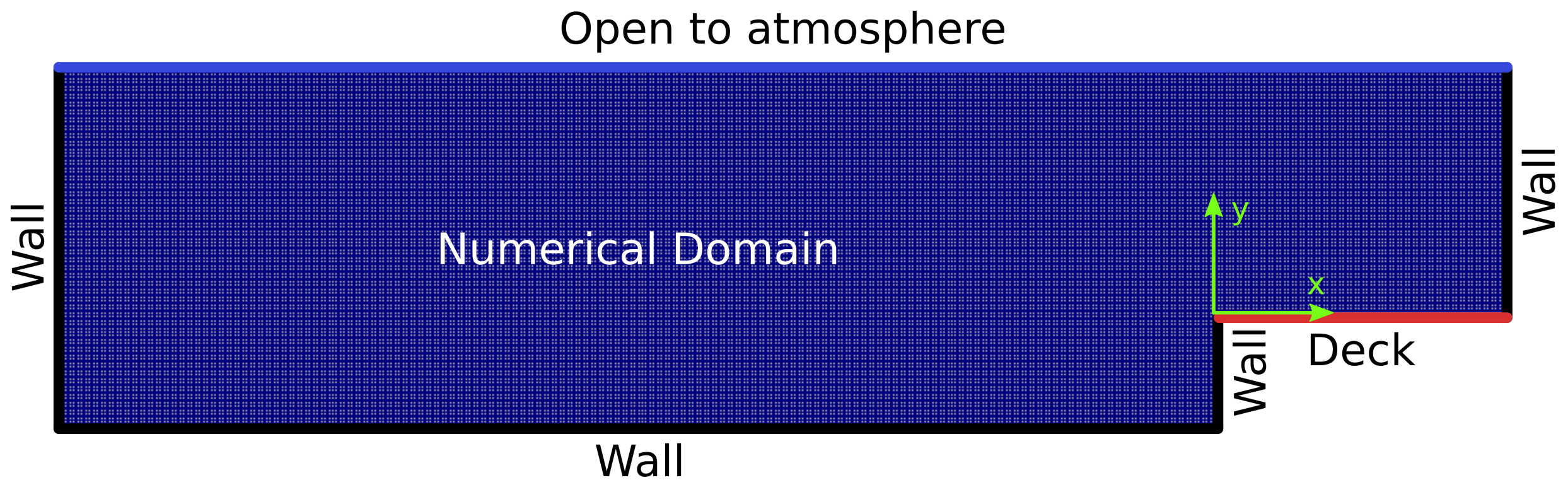
Figure 4.
Numerical domain for the dam-break simulations.

Figure 5.
Free surface elevation relative error as a function of time.

Figure 6.
Comparison between the vertical loads of the experiment and the numerical simulation.

Figure 7.
Sketch of the configuration of the study cases analysed numerically.

Figure 8.
Mean y+ values. (a) Roughness cases. (b) Deck length cases.

Figure 9.
Effect of deck roughness on shipping water velocities. (a) Time series of horizontal velocity () at the deck edge for different roughnesses. (b) Time series of vertical velocity () close to the deck wall for different roughnesses.
Figure 9.
Effect of deck roughness on shipping water velocities. (a) Time series of horizontal velocity () at the deck edge for different roughnesses. (b) Time series of vertical velocity () close to the deck wall for different roughnesses.

Figure 10.
Effect of deck roughness on shipping water loads. (a) Time series of vertical loads per unit length over the complete deck () for different roughnesses. (b) Time series of horizontal loads per unit length on the deck wall () for different roughnesses.
Figure 10.
Effect of deck roughness on shipping water loads. (a) Time series of vertical loads per unit length over the complete deck () for different roughnesses. (b) Time series of horizontal loads per unit length on the deck wall () for different roughnesses.

Figure 11.
Effect of deck length on shipping water velocities. (a) Time series of horizontal velocity () at the deck edge for different deck lengths. (b) Time series of vertical velocity () close to the deck wall for different deck lengths.
Figure 11.
Effect of deck length on shipping water velocities. (a) Time series of horizontal velocity () at the deck edge for different deck lengths. (b) Time series of vertical velocity () close to the deck wall for different deck lengths.

Figure 12.
Effect of deck length on shipping water loads. (a) Time series of vertical loads per unit length over the complete deck () for different deck lengths. (b) Time series of vertical loads per unit length over deck wall () for different deck lengths. (c) Maximum and loads found in (a,b) for all the study cases (L0–L5).

Figure 13.
Snapshots that represent the stages at which the maximum and loads ocurred during forward and backflow loading stages, for different deck lengths (cases L0–L5). Note that the domain was reduced from right to left, leaving the same distance for wave development in all cases.
Figure 13.
Snapshots that represent the stages at which the maximum and loads ocurred during forward and backflow loading stages, for different deck lengths (cases L0–L5). Note that the domain was reduced from right to left, leaving the same distance for wave development in all cases.


Table 1.
Transport properties of the fluid phases.
| Property | Water | Air |
|---|---|---|
| Density () | 1000 | 1 |
| Kinematic viscosity () | 1.01 × 10⁻⁶ | 1.51 × 10⁻⁵ |
| Surface tension () | 0.07 |
Table 2.
Characteristics of Mesh A, B, and C.
| Normalized Grid Spacing | Direction | Dimension (m) | Divisions | Cell Size (cm) | |
|---|---|---|---|---|---|
| Mesh A | 1 | X | 1.558/0.392 * | 619/156 * | 0.25 |
| Y | 0.15/0.325 * | 59/129 * | 0.25 | ||
| Mesh B | X | 1.558/0.392 * | 438/110 * | 0.36 | |
| Y | 0.15/0.325 * | 42/91 * | 0.36 | ||
| Mesh C | 2 | X | 1.558/0.392 * | 310/78 * | 0.50 |
| Y | 0.15/0.325 * | 30/65 * | 0.50 |
* Mesh region over the deck structure.
Table 3.
Study cases simulated with the CFD model.
| Study Case | (m) | Study Case | Deck Length (m) |
|---|---|---|---|
| R0 | 0.0 | L0 | 0.3920 |
| R1 | 0.005 | L1 | 0.3267 |
| R2 | 0.010 | L2 | 0.2613 |
| R3 | 0.015 | L3 | 0.1960 |
| R4 | 0.020 | L4 | 0.1307 |
| R5 | 0.025 | L5 | 0.0653 |
Publisher’s Note: MDPI stays neutral with regard to jurisdictional claims in published maps and institutional affiliations. |
© 2021 by the authors. Licensee MDPI, Basel, Switzerland. This article is an open access article distributed under the terms and conditions of the Creative Commons Attribution (CC BY) license (https://creativecommons.org/licenses/by/4.0/).
Share and Cite
MDPI and ACS Style
Rodríguez-Ocampo, P.E.; Fontes, J.V.H.; Ring, M.; Mendoza, E.; Silva, R. A CFD Numerical Study to Evaluate the Effect of Deck Roughness and Length on Shipping Water Loading. Water 2021, 13, 2063. https://doi.org/10.3390/w13152063
AMA Style
Rodríguez-Ocampo PE, Fontes JVH, Ring M, Mendoza E, Silva R. A CFD Numerical Study to Evaluate the Effect of Deck Roughness and Length on Shipping Water Loading. Water. 2021; 13(15):2063. https://doi.org/10.3390/w13152063
Chicago/Turabian StyleRodríguez-Ocampo, Paola E., Jassiel V. H. Fontes, Michael Ring, Edgar Mendoza, and Rodolfo Silva. 2021. "A CFD Numerical Study to Evaluate the Effect of Deck Roughness and Length on Shipping Water Loading" Water 13, no. 15: 2063. https://doi.org/10.3390/w13152063
Note that from the first issue of 2016, this journal uses article numbers instead of page numbers. See further details here.