
The Grids Python Tool for Querying Spatiotemporal Multidimensional Water Data
by
 , , , and
Riley Chad Hales
* ,
,
Everett James Nelson
,
Gustavious P. Williams
,
Norman Jones
 ,
,
Daniel P. Ames
and
J. Enoch Jones
Department of Civil and Environmental Engineering, Brigham Young University, Provo, UT 84602, USA
*
Author to whom correspondence should be addressed.
Water 2021, 13(15), 2066; https://doi.org/10.3390/w13152066
Submission received: 20 May 2021
/
Revised: 21 July 2021
/
Accepted: 27 July 2021
/
Published: 29 July 2021
(This article belongs to the Special Issue Advances in Hydroinformatics for Water Data Management and Analysis)
Abstract
:Scientific datasets from global-scale earth science models and remote sensing instruments are becoming available at greater spatial and temporal resolutions with shorter lag times. Water data are frequently stored as multidimensional arrays, also called gridded or raster data, and span two or three spatial dimensions, the time dimension, and other dimensions which vary by the specific dataset. Water engineers and scientists need these data as inputs for models and generate data in these formats as results. A myriad of file formats and organizational conventions exist for storing these array datasets. The variety does not make the data unusable but does add considerable difficulty in using them because the structure can vary. These storage formats are largely incompatible with common geographic information system (GIS) software. This introduces additional complexity in extracting values, analyzing results, and otherwise working with multidimensional data since they are often spatial data. We present a Python package which provides a central interface for efficient access to multidimensional water data regardless of the file format. This research builds on and unifies existing file formats and software rather than suggesting entirely new alternatives. We present a summary of the code design and validate the results using common water-related datasets and software.
1. Introduction
1.1. Background
For many numerical models in the earth sciences, an important part of the input data is a time series of gridded spatial data representing a phenomenon at sequential time steps. Water models typically need a time series of values for input variables such as soil moisture, precipitation, surface runoff, or evapotranspiration; each of which are generated, archived, and distributed as raster datasets on large spatial or temporal domains [1,2]. Furthermore, the results of these models often produce additional multidimensional datasets such as are produced by MODFLOW or SRH-2D models and the United States National Water Model [3,4,5]. These raster data, also called gridded data or multidimensional array data, are data stored in an array structure and represent the variation of a variable with respect to each of its dimensions. In the case of spatial data, the raster stores the fluctuation of data across space. Spatiotemporal data vary across both space and time. In addition to the spatial and temporal dimensions, other data dimensions, such as model realizations or ensemble numbers in stochastic models, may also be used.
The global scientific community has been trending towards generating and sharing more of these kinds of datasets. One evidence of this is the expanding global repository of Earth observation satellite and remote sensing data and numerical model results. The National Oceanic and Atmospheric Administration (NOAA) alone produces on the order of tens of terabytes of observation and model results data each day, the majority of which are raster data [6]. The repository for the National Aeronautics and Space Administration (NASA) Landsat dataset measures approximately three petabytes of multidimensional raster data and grows by approximately 700 GB every day [7].
In the case of vector spatiotemporal data, data represented by a point, line, or polygon, the spatial geometry and the time series observations are recorded separately. There are many standards for file formats to store the geometry component including the Esri Shapefile, Geographic JavaScript Object Notation (GeoJSON), and Keyhole Markup Language (KML). There is a small number of standards for sharing time series observations associated with the vector described spatial geometries. One such standard is the Observations Data Model (ODM) which is an SQL database schema for sharing point data and metadata [8]. The Consortium of Universities for the Advancement of Hydrologic Sciences Inc (CUAHSI), the Open Geospatial Consortium (OGC), and the World Meteorological Organization (WMO) have produced a series of coding packages, web apps, data services and standards, and other kinds of software which build on the ODM schema and common standards [8,9,10,11].
Multidimensional data, by contrast, are produced and stored in many formats that vary greatly in purpose, capabilities, functionality, and usability. These include raster formats traditionally used for image data such as Bitmap (BMP), Portable Network Graphics (PNG), and Joint Photographic Experts Group (JPEG); raster formats generally used for multiple “bands” of data, variables sharing the same grid structure, such as Geographic Tagged Image File Format (GeoTIFF) and Gridded Binary (GRIB); and raster formats used to store any n-dimensional array such as the Network Common Data Form (NetCDF), and Hierarchical Data Format (HDF) [12,13,14,15]. None of these formats specifically target time series of observations which gives rise to variability in how the data are labeled and organized within these file formats. Various organizations have developed their own standards to attempt to unify that variety by defining a convention for naming and organizing variables, metadata, dimensions, and other information in the files. The most prominent multidimensional dataset standards are the Climate and Forecast Conventions (CF Conventions) [16].
Research agencies and data producers typically adopt a particular format and organization convention for generating and disseminating data based on tradition or convenience in the computing workflow. For instance, the NASA Global Land Data Assimilation System (GLDAS) and the NOAA National Water Model (NWM) are distributed in the NetCDF format, while the NOAA Global Forecast System (GFS) and the European Centre for Medium-Range Weather Forecasting’s (ECMWF) Hydrology Tiled ECMWF Scheme for Surface Exchanges over Land (HTESSEL) land surface model data are distributed in GRIB format [5,17,18,19].
A water scientist is often interested in only a spatial and temporal subset from the complete archive which corresponds to their area of interest. These subsets are defined as points or multidimensional regions of the multidimensional array space, ℝn. That small region might be represented by a polygon in the two spatial dimensions, data between a start and end time along the temporal dimension, an average across the several ensemble members, and so forth. Variety in data formats, organizational conventions, and adherence to conventions makes obtaining and extracting subsets from any of these gridded data file formats more difficult. These are challenging problems which, if not addressed, limit how useful the data are to water scientists. There are several options for retrieving subsets from multidimensional datasets including using alternate file formats, using Geographic Information System (GIS) software or geoprocessing scripts, and using web services. Each of these solutions has its strengths and weaknesses described in the following subsections.
1.2. New File Formats and Conventions
Several alternate data models, file formats and companion organization conventions have been suggested. Each attempt to address the difficulty in retrieving data from the files or to unify how raster data are stored and shared. For example, SciDB is a relational database model developed for storing and processing multidimensional array data [20]. Additionally, Zarr is a file format ideal for storing compressed and chunked arrays with particular benefits for cloud computing environments (https://zarr.readthedocs.io/en/stable/ (accessed on 4 May 2021)). Each of these alternatives provides an improvement over the file format that it was intended to replace. While these alternate formats are useful for the improvements that they offer, current systems continue to generate terabytes of data every day in a variety of formats. Data consumers would need to download and convert their data before receiving the benefits of the new format. Downloading and converting data requires significant time and computing power in addition to computing expertise in the old and new file formats. As such, these novel data structures and conventions are primarily beneficial to a specific data producer or user rather than resolving the broader issue of variability in data formats and this often simply results in one more option.
1.3. GIS Software
The two core technologies for processing geospatial data are the Geospatial Data Abstraction Library (GDAL), and the PROJ library [21,22]. The GDAL has extensive support for querying raster files of many formats if they have exactly two dimensions that conform to a standard coordinate reference system (CRS). However, it has extremely limited support for rasters with three or more dimensions. The GDAL can operate on some NetCDF data if the data conform to the Climate and Forecast (CF) conventions [14]. The GDAL also supports reading and writing GRIB and HDF data if the data have certain encodings and metadata [20]. Common GIS software utilize these libraries and may inherit some support for these data formats. However, A GIS-based solution will generally be tied to the desktop installation environment of the software which is not easily transferable to other computing environments, such as a web application or web server. Additionally, GIS software may have licensing and cost restrictions related to their use. These two limitations make GIS-based solutions less than ideal for addressing the original data access problem since a GIS is rarely the only software required in a scientific computing workflow.
1.4. Web Services
Repositories of gridded datasets often become so large that the sheer volume of data makes transferring and processing them impractical. One solution to this big data problem involves the use of a data service. Data services are usually provided by the data generator and offer the most recent and updated version of the dataset with short lag times. The two pertinent kinds of data services for addressing the gridded data problem are processing or querying services and cloud computing platforms. Services are generally quick and eliminate data transfer overhead. The tradeoff is that the data service usually has a limited and predetermined set of functions available. Users generally still need programming experience and knowledge of a wide range of file formats but do not need to solve the data management problems that make raster data difficult to use. Both options are only applicable when the dataset’s generator has chosen to develop, deploy, and maintain the service. As this is not available for all datasets, it is not likely to satisfy all data consumers and data products.
Data processing services range in complexity from performing fast and simple queries of datasets to complex geospatial processing operations. Processing services have standards for formatting requests to the service and for the responses returned. Users send requests to the service provider which performs the specified operation using their copies of data and computing resources. When the job is finished, the provider sends the result back to the user. A common data service for simple queries is the Open-source Project for a Network Data Access Protocol (OPeNDAP) [23]. OPeNDAP is a RESTful data service that accepts queries for values from points or bounding boxes and returns the corresponding values in plain text format [24]. Other relevant examples are the Open Geospatial Consortium (OGC) Web Processing Service (WPS), the open-source standard for a geospatial web processing service, and the recently released openEO (open Earth observation) standard developed by a European Commission Research and Innovation program. Both the OGC WPS and openEO define a standard series of commands, known as an Application Programming Interface (API), which can be adapted to perform a wide range of functions and support solving many problems. Some researchers have already developed a custom implementation of the OGC WPS to perform time series analysis with their data [25]. The most prominent data processing Platform as a Service (PaaS) is Google Earth Engine which offers free or low-cost access to cloud computing resources and a large catalog of Earth observation datasets [26].
1.5. Proposed Solution
We evaluated these options on six criteria. These criteria include the following: does the solution (1) require bulk downloads of datasets, use data services, or both, (2) work on many file formats, (3) work on any public data product, (4) require programming or developing custom scripts, (5) work in many computing environments (e.g., personal computers, web servers, web processing services) (6) require subscriptions, licenses, or other costs. The results are summarized in Table 1. Each of these options partially fills the need but has limitations. Ideally, the solution to this data access problem would favorably meet all six of the criteria
This paper presents the design and development of a new method and its implementation in a Python package that addresses the practical difficulties in accessing, acquiring, and using gridded data in the water domain that stem from the lack of standards and the many competing formats. Specifically, our work promotes better access and processing capabilities for multidimensional gridded data in a variety of standard file formats with a focus on use within hydrology and water resources applications. As there are already many competing file formats, access software, and data conventions, we developed our method to build on existing technology and unify existing conventions rather than developing or proposing replacement standards. Our goals for developing this method and software include:
- It should be interoperable across existing multidimensional data file formats and appropriate web service technologies rather than create more variability;
- It should be free and open source, simple to use, and well documented to promote ease of access and distribution;
- It should be able to extract time series from gridded datasets at various spatial geometries including at a minimum: points, bounding boxes, and polygon shapes; and
- It should work in common scientific computing environments such as personal computers, cloud computers, and applicable web apps and services.
The remainder of this paper presents the development of the novel method, results of code performance tests and case studies, and conclusions and recommendations derived from the research.
2. Materials and Methods
2.1. Conceptually Handling N-dimensional Data
Multidimensional datasets can be difficult to understand and conceptualize when they contain more than three dimensions since visualizing more than three dimensions is challenging. The difficulty is augmented when the terminology for referencing these data is not clearly defined and may not be known or understood. We offer the following definitions consistent with the design of multidimensional data files and conventions such as the CF Conventions [16,27].
A dimension is a parameter for which data are collected which is independent of all other parameters (e.g., an independent variable). The most common dimensions for scientific data sets are the three mutually orthogonal spatial directions (e.g., X, Y, Z in cartesian coordinate space or longitude, latitude, elevation in geographic spatial coordinates), time, and model ensemble number or realization. Dimensions have names and a size which is an integer value that determines how many measurement intervals exist along that axis.
A variable is a set of data values which were observed, measured, or generated by a computational model. The variable is a function of some number of dimensions (e.g., a dependent variable). The number of dimensions determines the shape of the variable array. A variable has a measurement for each step across each dimension or axis. Consider a variable array which is a function of the three spatial dimensions, X, Y and Z. Every (X, Y) location has measurements at several Z values and every Z value has variable data across many combinations of (X, Y) coordinates. Examples of variables in multidimensional datasets include air temperature, precipitation rate, depth to groundwater and pixel color. A coordinate variable is a special variable which depends on only one dimension and holds the numerical values along that dimension where data were measured or computed. For example, a time dimension might have a size of three and the coordinate variable could contain the values 1 January, 2 January, and 3 January.
Consider a dataset with three dimensions, longitude, latitude, and time. The size of longitude is 360, the size of latitude is 181, and the size of time is 100. The coordinate variable for longitude is a one-dimensional array containing the integers from −180 to 179 and the coordinate variable for latitude is a one-dimensional array containing the integers from −90 to 90. The time coordinate variable is a one-dimensional array of datetime stamps for the first 100 days of the year 2021 at noon. This dataset could have a wind speed variable which is a function of longitude, latitude, and time and therefore has an array shape of (360, 181, 100). The total number of cells in that array is equal to the product of all the dimension sizes together.
2.2. Development Environment
We developed a new Python package called Grids to provide an efficient and flexible way to access gridded data in a variety of file formats and meet our objectives. Other software or coding packages exist which perform similar functions but with less query options and file format support (for instance, the Integrated Data Viewer (IDV) desktop software, the gstools python package [28], or the NetCDF Subset Service web server software [29]). We chose to develop this as a standalone Python package rather than an addition to existing package because we want Grids to solve the data access problem generally without being limited by the purposes or development strategies of other python packages. The approach outlined herein may be suitable for additions to existing packages or software in the future.
We developed Grids as a Python package because Python is common in scientific computing and available in a wide range of computing environments. Python is also feature rich with packages for computing statistics, performing GIS operations, accessing databases, and creating web apps. We distribute the Grids code as a licensed, open-source package to make it easier to integrate into scientific computing environments and be used more widely as compared to a module or plug-in for existing proprietary software such as GIS programs. Not all geoscientists use the same software and rarely does any single software address all a scientist’s needs. By developing Grids as a Python package, we hope more geoscientists will be able to integrate these capabilities into their work.
2.3. Software Workflow
The workflow to extract a subset of data from a multidimensional, spatiotemporal file consists of eight general steps:
- Programmatically “open” the file for reading.
- Read and interpret the file metadata including the names of the variables, the names and order of dimensions, and identifying which dimensions correspond to spatial and temporal axes.
- Read the values of the coordinate variable for each dimension used by the variable of interest.
- Identify the cells of the arrays corresponding to the area of interest by comparing the spatial, temporal, or other coordinate values to the user-specified coordinates.
- Read the values of interest from the file in the identified cells.
- Read the time values corresponding to the extracted variable values.
- Format the extracted data into a tabular structure.
- Programmatically “close” the file.
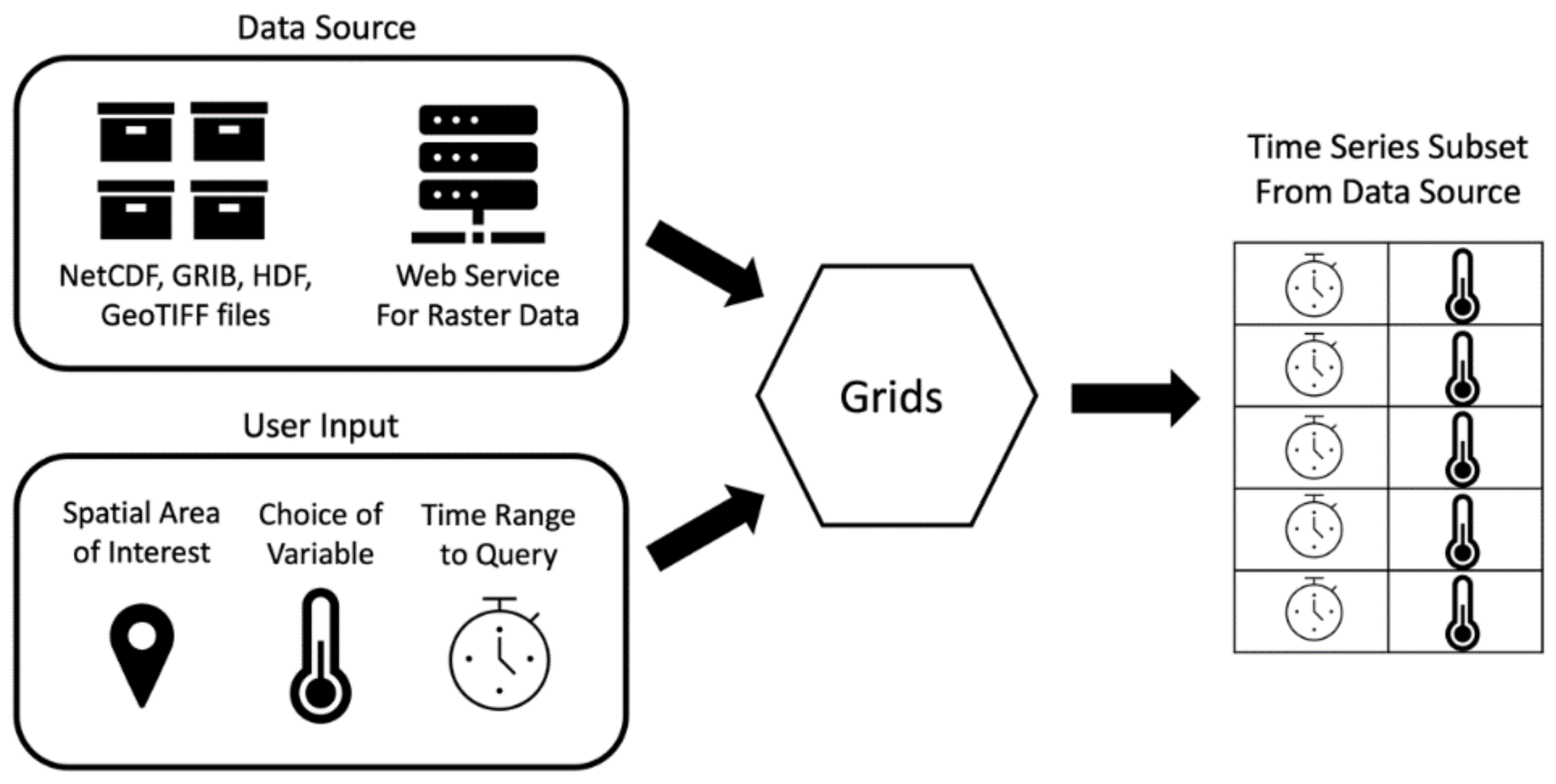
The Grids package implements these steps in a software architecture diagrammed in Figure 1. The Grids package code accepts a data source and user inputs and returns the extracted time series in a tabular structure. In steps one and eight, Grids interacts with the data source, which is the unique file format used for the data. In steps two through six, Grids uses inputs from the user, such as variable names, spatial locations, and time ranges, to extract a subset of data from the files. In step seven, Grids outputs the time series in the tabular Pandas DataFrame structure and returns this object for the user to process, save, or reformat as necessary [30]. As shown in Figure 1, the eight-step process for extracting a subset of time series data from a gridded dataset simplifies to the data source, user provided inputs, a tool which executes the querying for the data source, and an output.
2.4. Connecting to Data Sources
The workflow to extract time series subsets from a dataset generally begins with downloading copies of a dataset. Gridded, timeseries datasets are often so large in file size or updated frequently enough that this step can become difficult and impractical. The inefficiencies inherent in the downloading process can be minimized by taking advantage of web services that allow the user to access and retrieve data subsets without downloading the entire dataset. We chose to begin by targeting the OPeNDAP data service because it is a mature software and available through many web servers for multidimensional datasets [24]. When an OPeNDAP service is available for a dataset, Grids can query the data service to obtain the values corresponding to the user’s input.
Grids can directly interface with gridded data files stored on a local directory when web services are not available. To interface with each file format, we used the definitive open-source Python packages for reading and writing any given file format. They include NetCDF4, Cfgrib, H5py, and Rasterio which read NetCDF, GRIB, HDF, and GeoTIFF files, respectively [15,31,32,33,34]. Grids abstracts these differences away, allowing a common access interface to each file format. We designed Grids to provide a single set of functions which internally use the appropriate Python package for each format.
These Python packages used to read data are a modular component of Grids so additional packages can be included to expand Grids’ file format support. For instance, we added support for Pygrib which can read many GRIB files as binary messages. This is useful when the GRIB data are not properly labeled or organized and cannot be appropriately read through the Cfgrib package. While Pygrib is not the definitive package for a given data set, we noted its ability to read more datasets and provide performance improvements in some cases [35]. This modular design allows for flexibility so end users can specify which Python package to use as the file reading engine according to their requirements. Table 2 lists the currently included packages and the file formats they support.
2.5. Extracting Values by Comparing to Coordinate Values
Grids extracts time series data from n-dimensional data series by reducing them to a one-dimensional time series with one value per time step. The reduction method depends on whether the location of interest is a single point or a multidimensional region. If the location of interest is a single point, or a single array cell, Grids extracts the value contained in that cell of the array at each time step and returns this series, so no reduction is required. When the location of interest is many cells within the array, such as a two-dimensional area, three-dimensional volume, or region in higher dimensional space, the many values are reduced to a single value by computing a summary statistic value representative of the many cells. The statistic could be the average, median, maximum, minimum, standard deviation, or a percentile depending on what makes most sense for the datasets and use case.
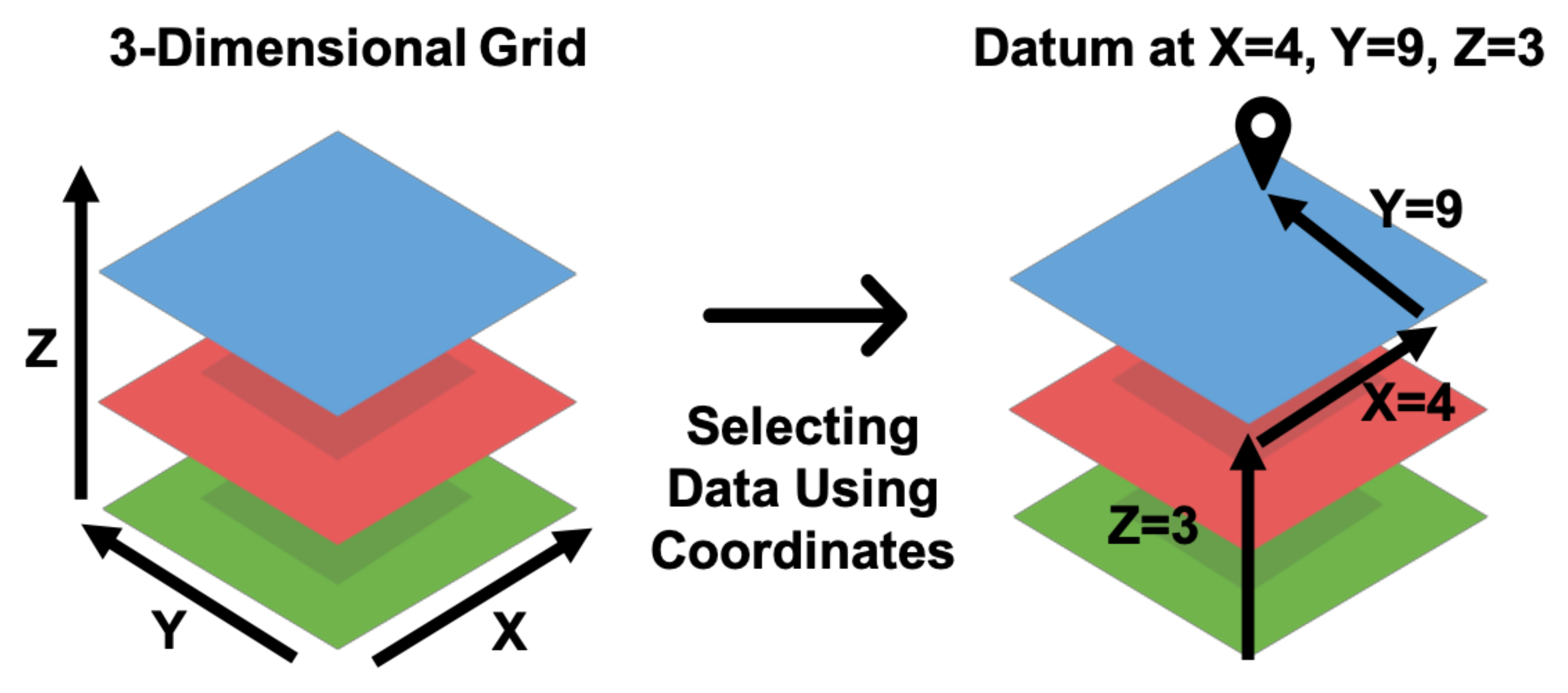
A visual representation of the process to identify subsets of a three-dimensional array using coordinates is shown in Figure 2. For example, the GFS data product is a four-dimensional array spanning three spatial dimensions, latitude, longitude, and elevation, as well as the time dimension. Extracting a time series of values from GFS data requires a coordinate pair of latitude, longitude, and elevation for a point or two for the maximum and minimum corners of a bounding box. The bounding box is analogous to a rectangular prismatic shape in three dimensions with a base defined by the maximum and minimum latitudes and longitudes with a height defined by the maximum and minimum elevations (thus a volume). To identify the data within the files to extract, the coordinates (latitude, longitude, and elevation values) are mapped to the array cell or cells representing that multidimensional location using the spatial resolution and affine transformation of the data; both of which are readily determined via inspection of the coordinate variable values. For a given point or region (e.g., area for 2D, volume for three or more), Grids extracts the data in the array cell or cells for each time step and computes the appropriate statistical reduction (i.e., computing the median or mean). These extracted time and variable values are then organized in a tabular structure and returned.
Grids maps a specified volume to the data in the file but may map certain coordinates to points and others to ranges depending on the resolution of the dimensions. A set of minimum and maximum coordinates could map to the same cell if the distance between the minimum and maximum is less than the distance between grid points on that dimension. In other dimensions, the distance between coordinates may be larger than the resolution of that dimension. In this case, the queried coordinates are point data in one dimension while having a range in another. Grids would treat the query as a point, one cell, on the first dimension and range, multiple cells, requiring a statistical reduction on the other.
Due to the size of the files or for convenience in dissemination, some datasets are stored in multiple files across a dimension. Such is the case for GLDAS, NWM, GFS, and HTESSEL. All files contain results for each of the spatial dimensions and ensemble members but for only one time step. The time dimension is reconstructed by the combination of each file representing each time step. For these datasets, Grids can handle these datasets by repeating the querying steps for each file and combining the results from each file into the same tabular format.
Arrays of several different data dimensions store data in variables described by those dimensions. A dataset can have many dimensions with not all variables using the same dimensions or organized in the same order. Consider a multidimensional dataset which has five dimensions, X, Y, Z, time, and ensemble number. There might be three-dimensional variables which depend on the three spatial dimensions. One variable in the dataset may store arrays of information organized according to measurements made in the X-direction, followed by the y-direction, then the z-direction (i.e., X, Y, Z). Other variables may also be three dimensional but arrange their measurements according to the Z-dimension, followed by X and Y (i.e., Z, X, Y). Grids can query each of these variables.
Multiple variables may share the same dimensions and in the same order which yields arrays with identical structure or shape. For example, multi-spectral data have many bands for each cell, some measured and some computed. A simple 2D time-varying raster data could have temperature, humidity, soil moisture, or other values. If a user is only interested in soil moisture and temperature from the environmental data set over an area that includes nine cells (X, Y), Grids would extract data for these two variables at each time step, average the values for each variable over the nine cells, then move to the next time step. This results in a time series with two different variables at each time step.
2.6. Querying Higher Dimensional Data
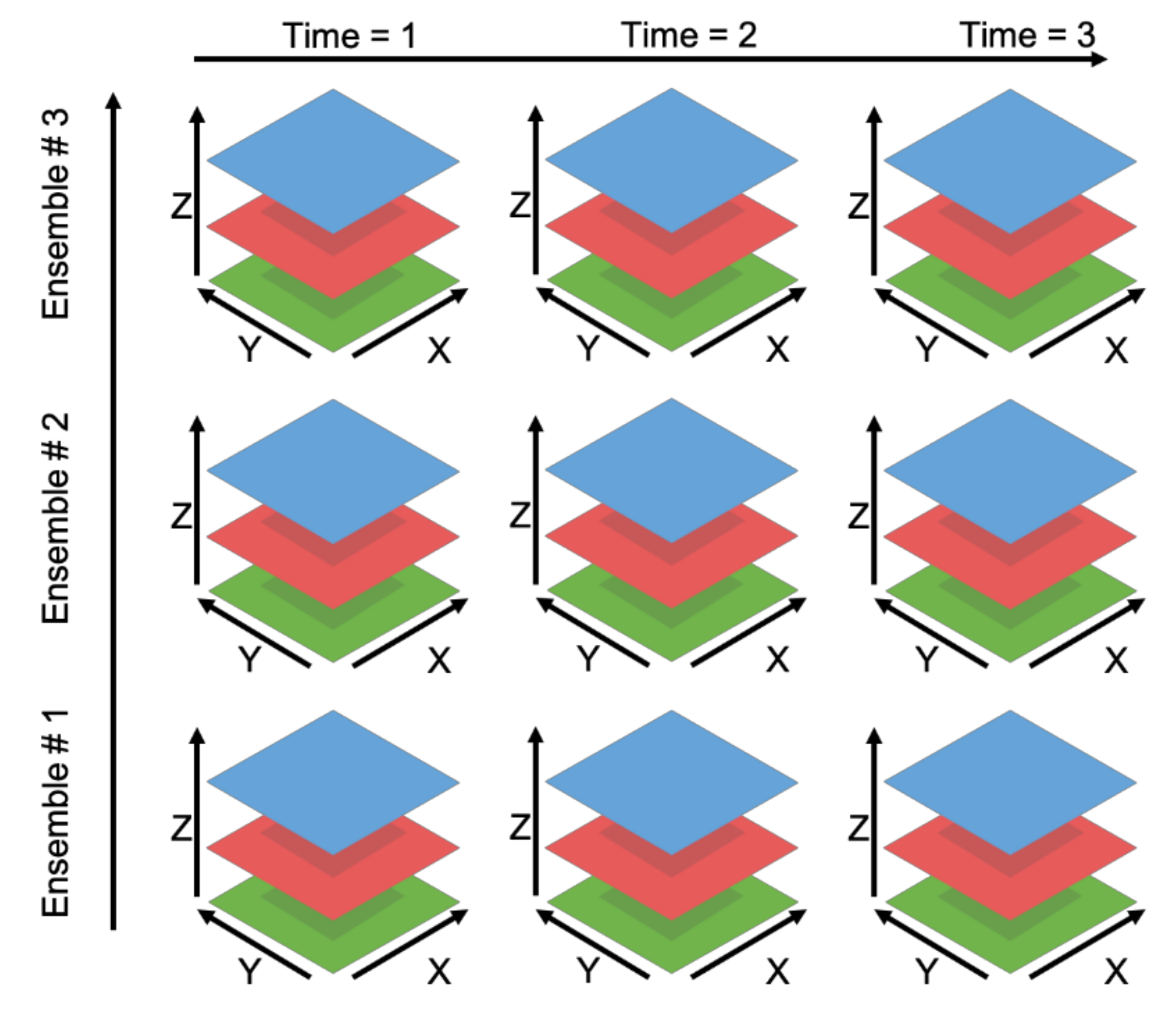
This procedure using coordinates scales to data of other dimensional sizes if the number of dimensions of the array is equal to the number of specified coordinates. The dimensions in datasets of more than three dimensions no longer correspond to an independent spatial dimension but can be traversed in the same fashion. Figure 3 presents a five-dimensional data set, ℝ5, which is a 3D spatial volume with three different realizations along the ensemble number dimension and three across the time dimension. In this instance, Grids uses the coordinates provided by the user to determine the proper subset in five dimensions in the same manner as was described with previous examples. The coordinate provided by the user is compared to the coordinate variable values stored in the file to identify the correct subset of the variable’s array. Those values are read from the multidimensional data file, formatted, and returned to the user.
2.7. Extracting Values within Boundaries Using Masks
In many cases, the subset of interest often does not correspond to a single point or a rectangular bounding box. Multidimensional spatial areas are often irregular 2D polygons such as a watershed or administrative boundary, or a 3D prism shape representing a volume. Each point on and within the polygon can be mapped to a location on the multidimensional grid following the same procedure as presented in the coordinate lookup method. However, such a lookup would be cumbersome to program and not as efficient as scripts using optimized algorithms such as are available in the GDAL for raster spatial data or NumPy for any n-dimensional array [22,36]. Depending on the resolution of the spatial dimensions and the size of the polygon of interest, a user might be interested in 1,000′s or 1,000,000′s of points in the multidimensional area.
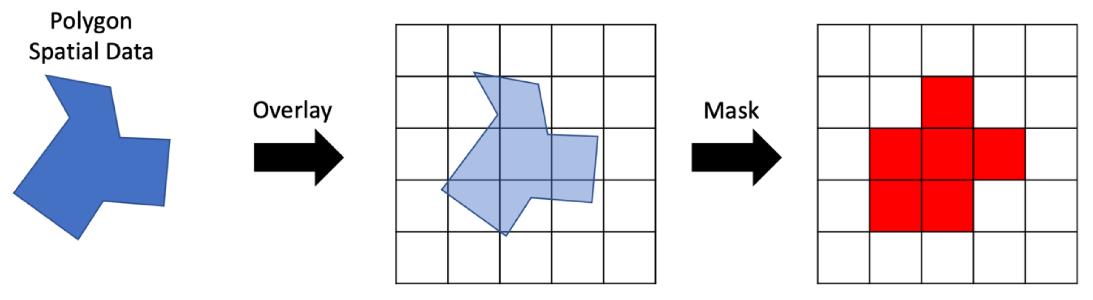
We can optimize queries on irregular polygon areas in spatial datasets by using a mask. A mask is a rasterized representation of the vector data It is an array with the same CRS as the variable to be queried. This means that the mask array has the same shape, extents, and resolution as the arrays within the multidimensional dataset that are being queried. The values are in the mask array are binary, 1 or 0, or boolean, true or false, indicating whether the cell should be selected or ignored.
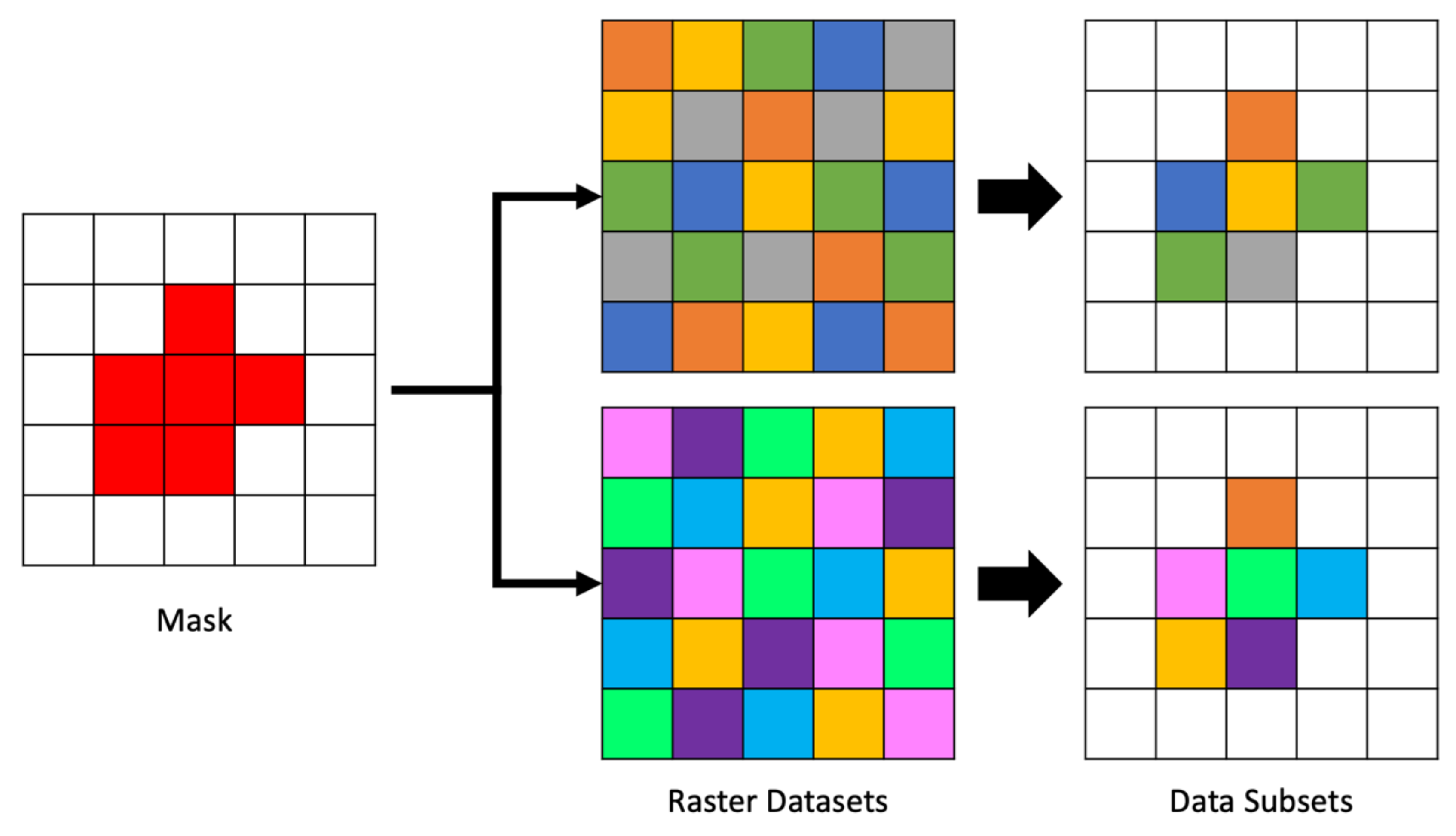
An example of the steps to create a raster mask for spatial data are shown in Figure 4 assuming a vector representation of the spatial area of interest and 2D spatial gridded data. The vector area is overlain on a blank array of the same shape and resolution as the data to be masked. Cells in the mask raster on the right were selected using a geoprocessing algorithm to compare the amount of area in each cell covered by the vector polygon. Cells covered more than 50% by the polygon were selected. The mask contains the values 0 or 1, shown as white and red, respectively in Figure 4. Where the mask has a 1, we retrieve the data, where it has a 0, we do not.
The mask array is created in advance of reading each file and then applied to each two-dimensional array segment as it is retrieved from the file. Though generating the mask is somewhat computationally expensive, our approach gains some efficiency by caching and reusing the mask. This means there is a fixed time cost to performing spatial querying operations regardless of the number of files and time steps. That is comparable to the fixed cost of identifying the array cell corresponding to queries for a set of coordinates. An example of applying a single mask to multiple datasets is shown in Figure 5. The mask, shown on the left of the figure is the same mask generated in Figure 4. The center of the figure shows two different arrays of data to be masked followed by the resulting cells selected by the mask to their right.
3. Results
3.1. Validation of Time Series Results
We evaluated the performance of the Grids tool with speed tests and case studies in extracting time series subsets with several datasets. The purpose of the tests is to evaluate the competency of the methods used in Grids as well as gauge the efficiency of the code. For these tests, we used long term forecast NWM files from May 2021, GLDAS version 2.1 3-hourly dataset from January to February 2020, and GFS data from January 2021. Characteristics of these datasets are summarized in Table 3. These data are frequently applied to water modeling applications such as GLDAS being used to train machine learning algorithms that predict groundwater levels [37,38,39,40]. As they are extensively used and have different numbers of dimensions, we felt these data were representative of many kinds of multidimensional data used in water modeling. We used a subset of the variables in the GFS dataset to keep the file sizes comparable to the NWM and GLDAS data, between 25 and 30 megabytes.
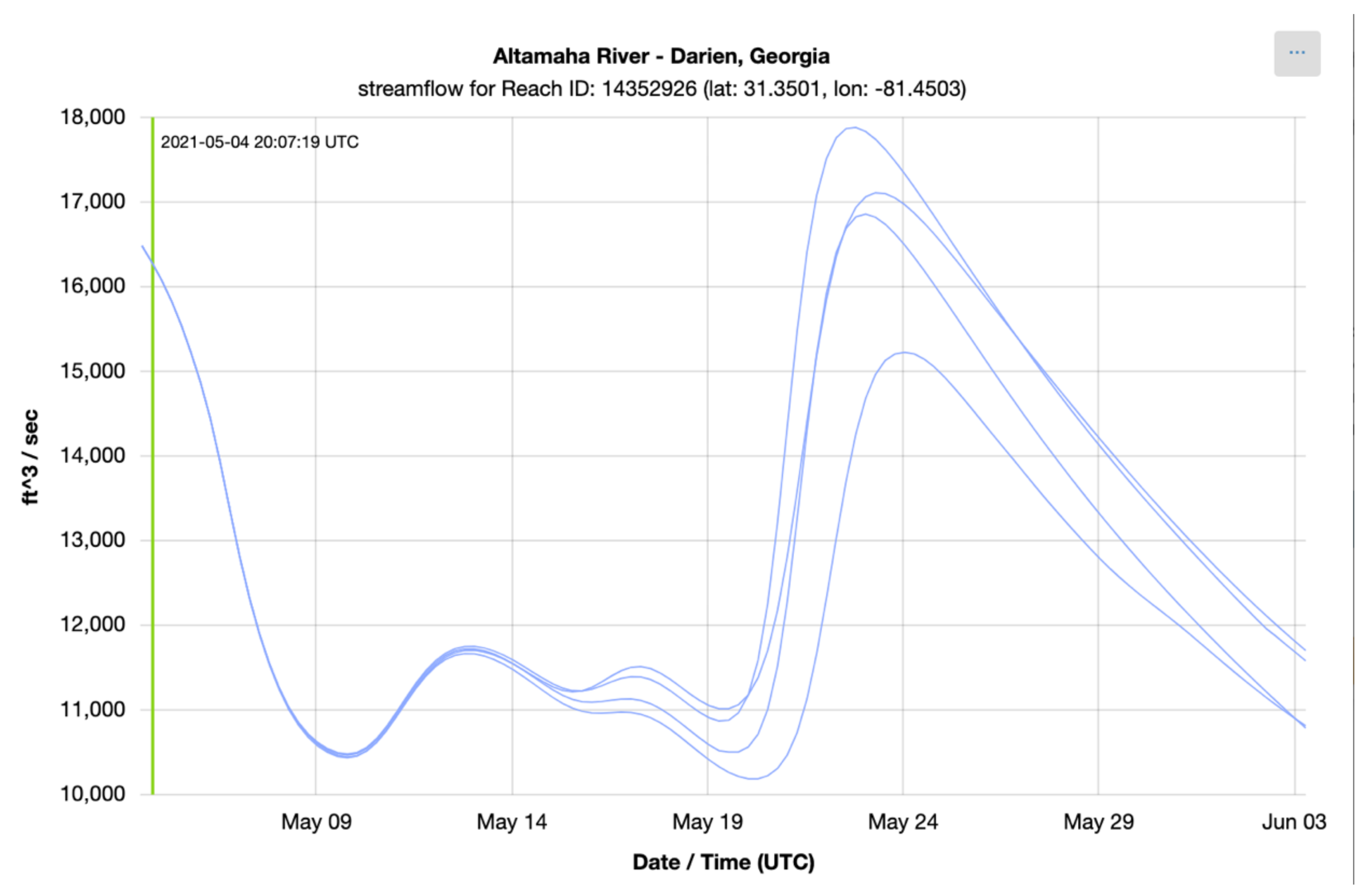
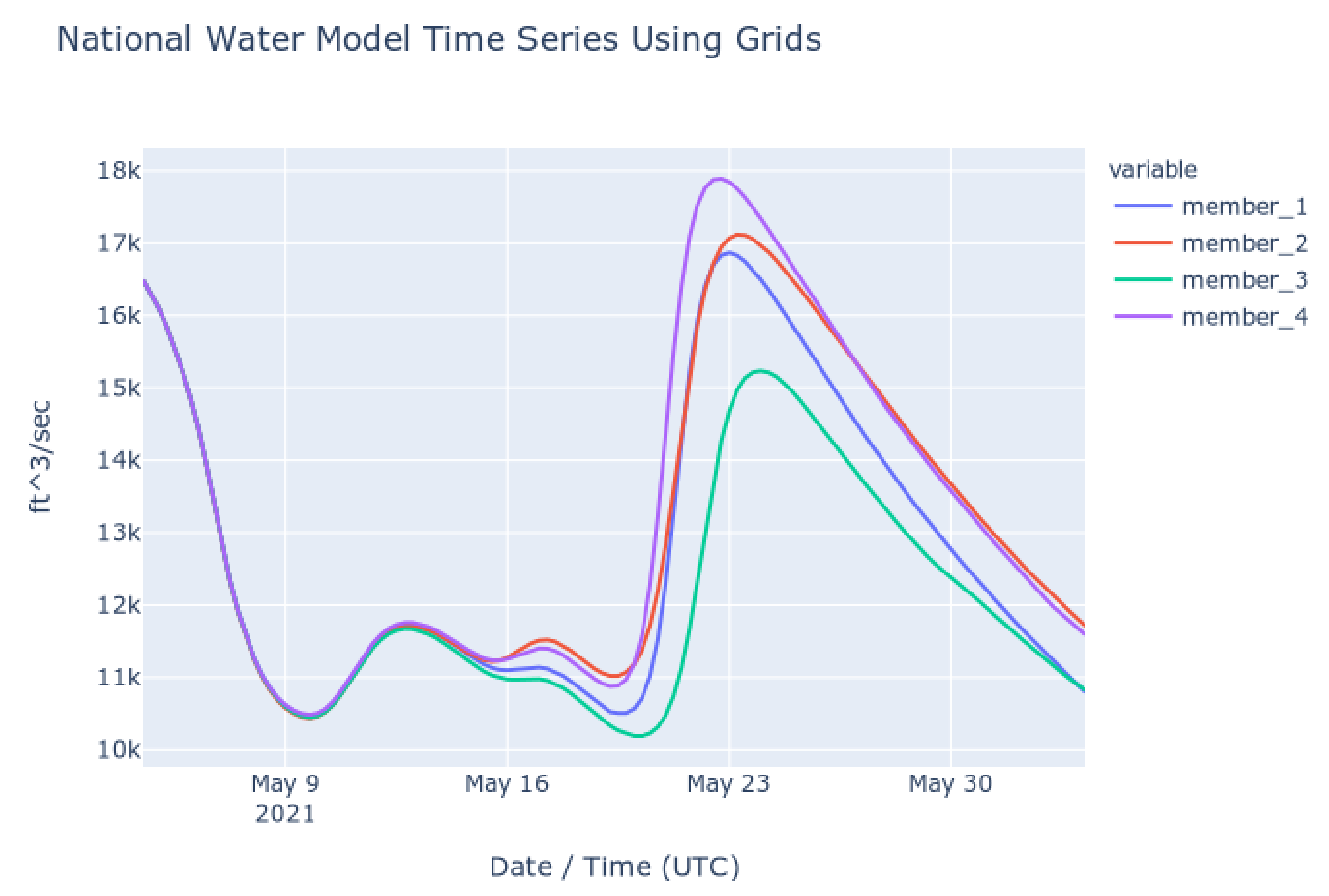
To check the accuracy of the results retrieved using Grids, we retrieved series from downloaded copies of the NWM multidimensional dataset (NetCDF) and compared them to results retrieved using the authoritative NWM web app [41]. The time series shown in the following plots show the NWM long term forecast generated 4 May 2021 06:00 UTC for the outlet of the Altamaha River in Darien, Georgia, United States. This forecast is for the following 30 days and is comprised of 4 ensemble members. Each member is plotted separately. Figure 6 shows the time series retrieved from the web app for the NWM provided by NOAA and Figure 7 shows the time series generated with downloaded copies of the NWM data and extracted using Grids (plots generated with Plotly) [42]. These figures show that the results from the authoritative web app for the NWM are identical to those retrieved using Grids.
3.2. Speed Performance on Local Datasets
For the first set of speed tests, we stored the datasets locally on the computer where the Grids code was executed. We measured the time taken to extract a series of values based on the file format and the size and type of subset being extracted. The independent variables to be compared are the file reading engine, and by extension the file type, and the type of query being performed which is analogous to the amount of data being queried and processed. We tested these two variables in a full factorial comparison which included all possible parameter combinations. As Grids currently only supports a limited number of file reading packages, these trials compare the differences in time between the several packages as if they were representative of all other packages for reading that format of data. This is may not be an accurate assumption and could be revisited after additional file readers are supported by Grids.
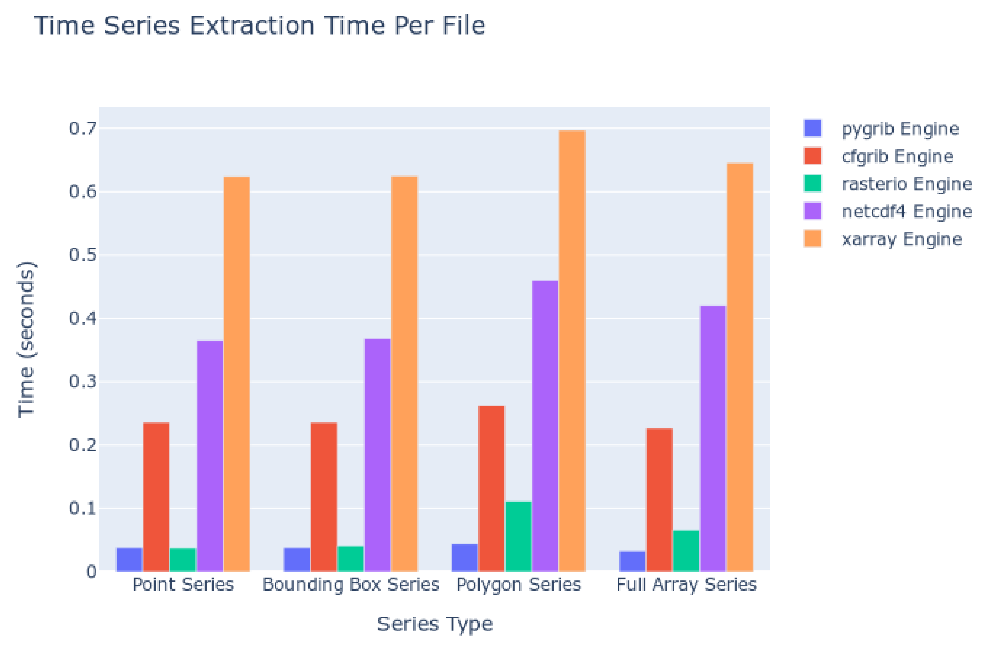
The kinds of queries executed were point queries, bounding boxes of a 2D spatial area across each time step, polygon queries using Esri Shapefiles and the masking process, and computing statistics for the entire 2D spatial array at each time step. The amount of data to read from disc and additional processing work (i.e., computing statistics for many cells) increases with each of those queries, in that order. The results are summarized in Figure 8. The computation time to extract the timeseries is shown with respect to the kind of extraction and the Python package used as the file reading engine. Smaller columns indicate faster read times and therefore more desirable performance.
We interpreted these data by comparing the file reading engine with the file formats supported (Table 2). These data indicate that for our test, the Pygrib engine, which supports reading only GRIB data, is the fastest, with an averaged time of less than 0.1 second per file in the series. The Rasterio engine, which reads GeoTIFF data, follows closely behind. The Cfgrib engine is next with average read times between 0.2 and 0.3 s. NetCDF and HDF data, as read by the NetCDF4 engine, come next with times ranging between 0.35 and 0.5 s, respectively. The slowest engine is the Xarray engine with read times of 0.6 s.
The trend in speeds matches the work performed by the engine to interpret the data and metadata within the files as a programming object in Python. Pygrib does the least work while Cfgrib, as implemented in Xarray, does the most work to try to match the arrays of data with a standard data model. Judging solely in terms of reading speed, the GRIB format performed the best. However, the GeoTIFF or NetCDF formats may be preferable to data generators or to end users since the GRIB format has other weaknesses such as loose organization rules as mentioned previously.
3.3. Speed Performance on Remote Data
For the second set of speed tests, we accessed data stored on a remote server. When retrieving data from a remote server, the time to extract subsets of data can vary significantly over repeated attempts with the same parameters. Some of the factors which influence the time include the internet upload and download bandwidth available on the client and cloud server, the computing load on the cloud location at the time the request is made, the amount of computing power available to the cloud service, and the amount of user authentication required. These tests used the Xarray package as the file reading engine since it has the capability of querying remote data sources. The remaining file reading packages currently wrapped by the Grids package are not able to read remote data sources, so the time results reported do not show variance across different file reading engines.
To minimize the variability due to these factors, we created an instance of the Thematic Realtime Environmental Distributed Data Services Data Server (THREDDS) on a stable cloud environment on a local network that we controlled [43]. THREDDS is software that creates web services, including OPeNDAP, for gridded datasets. For these tests, the THREDDS instance was only queried by code executing the performance tests and had ample computing resources and internet bandwidth available. This setup does not fully take advantage of all available cloud technologies for optimizing computing. Nevertheless, it approximates ideal conditions for a web server that might be queried with Grids. Table 4 summarizes the results of the speed test. As with the local datasets, the values of this table indicate total times and smaller values means faster speed and more desirable performance.
The approximate time per file queried is slightly above one second and is an average of 120 trials for each time series. The trials were repeated with several formats of data and the variance in measurements and average times were nearly identical. This suggests that the file format on the server had marginal impact on the results which is different from the results with local data source shown in Figure 8. Any difference in performance due to file formats is overwhelmed by the time to request and receive data through the internet. Table 4 shows that the extraction times are nearly uniform across the four kinds of queries tested. However, users could expect considerable variation in their measured times to extract values from remote servers in their applications because of the factors that affect web service performance already described. Additional optimizations or alternate procedures may be necessary if greater speeds are required for specific use cases.
3.4. GLDAS Web App Case Study
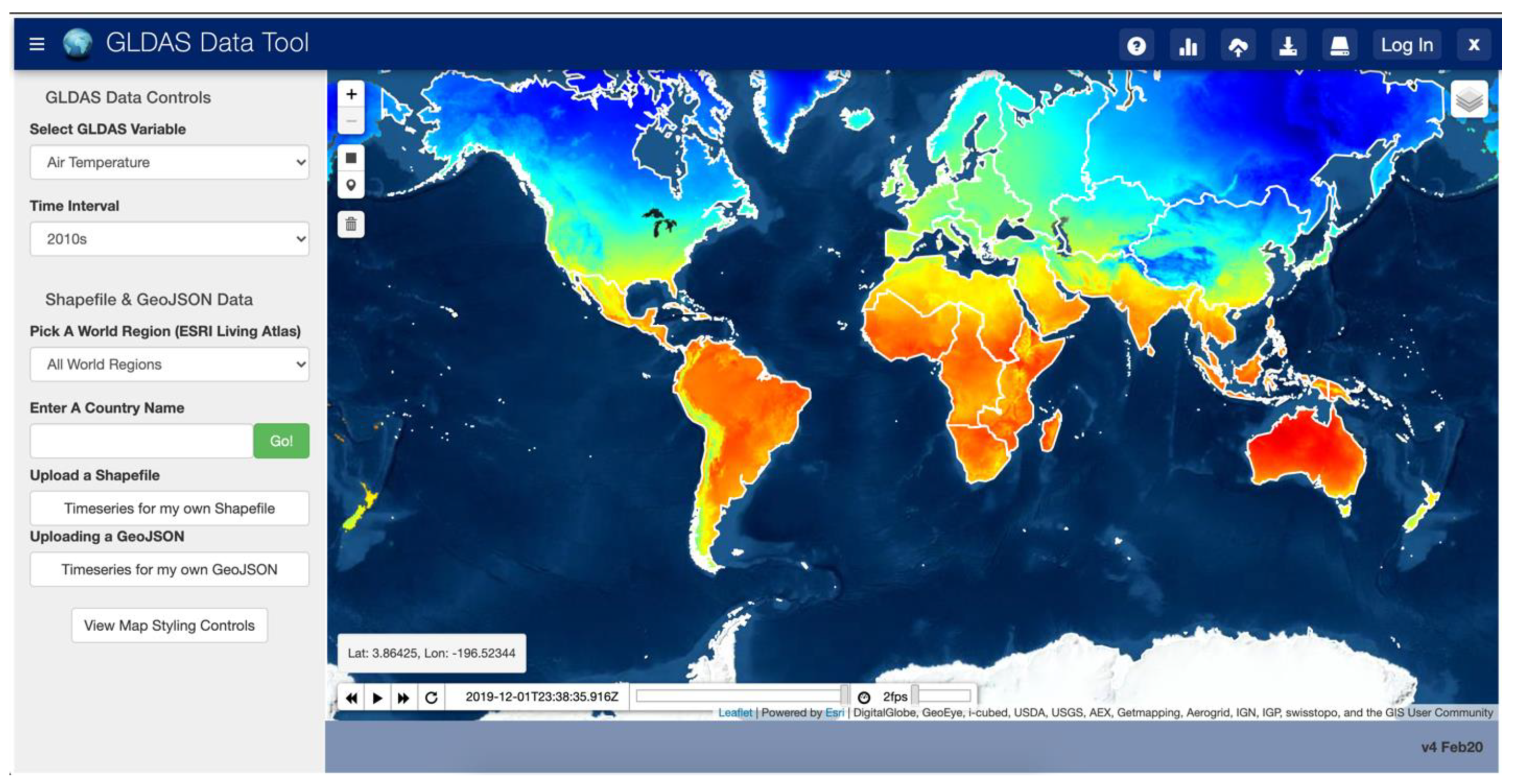
We developed a web app (the GLDAS App) to validate that the Grid tools work sufficiently fast for use in web environments. We developed The GLDAS App using the Tethys Platform. Tethys is an extension of the Django Model View Controller framework built on open-source Python code as well as PostgreSQL databases. Tethys Platform is intended to “lower the barrier” to creating web apps by providing a command line interface, template apps, code samples and examples, and documentation which helps users more quickly develop and deploy web apps [44]. It has been used for multiple applications that require access to multidimensional data sources which developed custom querying code and could have benefited from Grids [37,40,45]. We selected the NASA monthly-averaged GLDAS product as the gridded data for this test since the files have a small disc size, are easily accessible, and cover a long time period of more than 70 years. NASA provides an OPeNDaP web service for access to the GLDAS dataset. However, we did not build the GLDAS App to query that web service since we wanted to demonstrate that, given any multidimensional dataset, this code executes sufficiently fast to be used in web environments. This app accesses NetCDF files stored on the web server. The GLDAS product spans two spatial dimensions and one time dimension with approximately thirty variables spanning those three dimensions.
The GLDAS App design consists of a simple interface which shows an interactive map of the GLDAS data and a server backend which has a copy of the GLDAS NetCDF dataset. The interface prompts users for the GLDAS variable to query, the time range of values to query, and the location of interest using an interactive map. This query input is sent to the server backend which uses that information to build and execute Grids functions to extract the time series for the requested area and variable and returns a plot of the variable over time. Figure 9 shows the interface of this app.
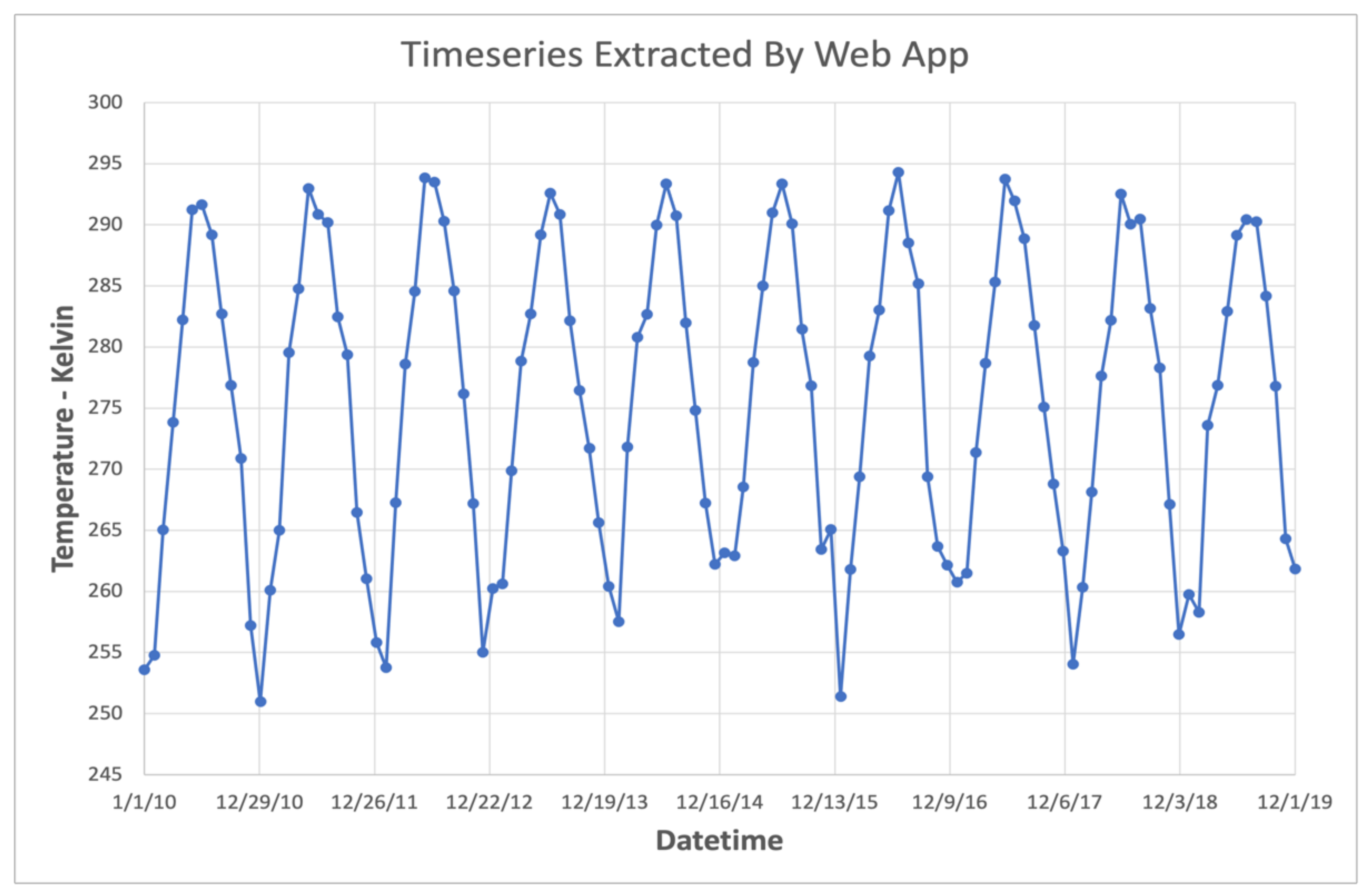
We deployed the GLDAS App on web servers in cloud environments on both Amazon Web Services and Microsoft Azure. On these cloud instances, users were successfully able to query time series of the GLDAS dataset with the available data range going from a few months up to, and including, the entire time range (January 1948 through the present). At the time of the tests, the web server which hosted the app was experiencing near-ideal conditions similar to the local network THREDDS instance described previously. Consequently, the measured speeds were comparable to those presented for an ideal web processing service. Figure 10 shows an example 10-year time series of air temperature extracted using the web interface to the GLDAS App.
3.5. WMO Web App Case Study
We developed a second web app for the WMO (the WMO App) to investigate the suitability of using Grids as a general-purpose tool for interacting with gridded data services rather than reading data files directly. This app accesses the OGC Web Mapping Service and OPeNDAP data service generated by THREDDS. This app is based on consuming THREDDS services since THREDDS can provide both mapping and data access services and it is relatively simple to create an instance of a THREDDS server. We developed the WMO App to promote broader access to multidimensional raster data common to national hydrometeorological services. We designed the WMO App to function similar to the GLDAS App except that the data source is an OPeNDAP data service rather than data which has been downloaded to the same server that hosts the web app.
We used this app to perform visualization and data retrieval from several datasets across various THREDDS instances. In these trials, the Grids code was generally successful at retrieving the time series data for the selected point or area. The trials revealed a few notable problems rooted in how data are organized. The problems can be addressed if the dataset is generated or reformatted to have a stronger adherence to existing conventions and through improving existing data conventions.
One such problem is that the datasets often do not strictly conform to spatial referencing rules. That is, they do not use a standard CRS. Multidimensional datasets often use a geographic coordinate system to organize spatial data such as the European Petroleum Survey Groups (EPSG) 4326 CRS. EPSG 4326 measures longitude from −180 and degrees to 180 degrees east and west of the prime meridian and measure latitude from −90 to 90 degrees from the equator. Many meteorological datasets, such as the GFS dataset, measures longitude from 0 to 360 degrees from the prime meridian. While this difference can be understood by a researcher and map generating software, most vector spatial datasets do not use this coordinate system. Reprojection tools are not readily available for every non-standard coordinate system. The poor adherence to organization and metadata conventions in some datasets further complicates programmatically determining the proper transformation. This irregularity does not make gridded data unusable, but it does inhibit direct integration with software based on standard geospatial libraries. Each deviation from standard geospatial conventions makes automatic interpretation and processing of data more difficult.
4. Discussion
The Grids Python package improves access to multidimensional raster data by providing simple tools for interacting with data stored in local files in several file formats or through web services. Grids interfaces with many Python packages to read those file formats. It is unique because it is applicable to many file formats and is available to many computing environments through Python package installers such as Pip. Grids achieves flexibility and efficiency through a design that minimizes required inputs from the user while being interoperable across data from many sources and formats. We have optimized Grids to reduce redundant computations and computing time. We presented speed tests and example web apps that show patterns of how the code performance varies with respect to the selected file format, the choice of file reading Python package, the way an area of interest is defined, and whether the data are being retrieved from local files or via a web service.
We tested Grids on additional datasets besides those presented. The datasets we used in these tests were exclusively small or medium size files of multidimensional data. Some data sets present additional challenges. For example, several Earth observation data products have file sizes reaching many gigabytes per file. These datasets are uniquely difficult to work with because of their size and require specialized computer infrastructure, such as is available through Google Earth Engine [26]. While Grids has been used on some larger datasets, it has not been thoroughly tested and therefore is not recommended as a specialized tool for handling datasets stored in extremely large files.
We found that the largest issue when using Grids was data storage conventions. Data should conform to organizational conventions to facilitate being queried programmatically and be compatible with web service software. While noncompliance to conventions does not make data unreadable or unusable, compliance to conventions allows for data to be easily used and understood by both human users and programs [26]. File formats differ on how rigidly they enforce data organization and how simply they can be programmatically queried. GeoTIFF data are the most rigid followed in order by NetCDF, GRIB, and HDF. Converging towards a common set of file formats and conventions allows for tools and methods, such as the Grids Python package, to access any dataset and therefore lowers barrier to accessing data. Even if the file format does not require it, we suggest that data generators choose to conform to standards to make wide data dissemination more accessible.
Further, we recommend that new data should be generated to conform with existing standards using existing file formats where possible. We recommend using the Climate and Forecast (CF) conventions and the NetCDF file format because it is already adopted by web service software, such as OPeNDAP and THREDDS, and NetCDF is a self-describing format [23,33]. New data should strictly conform to a standard CRS format and store that metadata appropriately. These practices move data toward being accessible by end users and their client software while avoiding the problems inherent to weakly defined data standards.
Data generators should consider offering a web service for visualization and data querying access where such is practical. This makes data easy to access with data tools such as Grids and to visualize through mapping engines. Data access and visualization services simplify the process to use datasets by minimizing or removing the need for scientists to transfer data in bulk before executing their models. Data consumers should take advantage of web services when appropriate to simplify their computing workflows.
Author Contributions
Conceptualization, methodology, software, analysis, investigation, and writing—original draft preparation, R.C.H.; writing—review and editing R.C.H., E.J.N., G.P.W., N.J. and D.P.A.; supervision, project administration, and funding acquisition E.J.N., G.P.W., N.J., and D.P.A.; software J.E.J. All authors have read and agreed to the published version of the manuscript.
Funding
This research was funded by the United States National Aeronautics and Space Administration (NASA), grant numbers 80NSCC18K0440 and 80NSSC20K0157.
Institutional Review Board Statement
Not applicable.
Informed Consent Statement
Not applicable.
Data Availability Statement
The Grids package is available for distribution via the Python Package Index (PYPI) and as source code via a GitHub repository at https://github.com/rileyhales/grids (accessed on 4 May 2021) [46]. Each distribution provides code documentation and examples as well as the most recently available speed test data. The source code of the demonstration web app for GLDAS data is available through GitHub at https://github.com/rileyhales/gldas (accessed on 4 May 2021) [47]. The source code of the demonstration web app for the WMO project is also available through GitHub at https://github.com/BYU-Hydroinformatics/Met-Data-Explorer (accessed on 4 May 2021) [48]. Installation instructions for the specialized Django framework, Tethys, are referenced from the GitHub repositories for the web apps.
Acknowledgments
We acknowledge the support of Brigham Young University’s (BYU) Civil and Environmental Engineering Department and the many researchers at BYU who collaborated and supported this work.
Conflicts of Interest
The authors declare no conflict of interest. The funders had no role in the design of the study; in the collection, analyses, or interpretation of data; in the writing of the manuscript, or in the decision to publish the results.
References
- Dieulin, C.; Mahé, G.; Paturel, J.-E.; Ejjiyar, S.; Tramblay, Y.; Rouché, N.; EL Mansouri, B. A New 60-Year 1940/1999 Monthly-Gridded Rainfall Data Set for Africa. Water 2019, 11, 387. [Google Scholar] [CrossRef] [Green Version]
- Asadi, H.; Shahedi, K.; Jarihani, B.; Sidle, R.C. Rainfall-Runoff Modelling Using Hydrological Connectivity Index and Artificial Neural Network Approach. Water 2019, 11, 212. [Google Scholar] [CrossRef] [Green Version]
- Langevin, C.D.; Hughes, J.D.; Banta, E.R.; Niswonger, R.G.; Panday, S.; Provost, A.M. Documentation for the MODFLOW 6 Groundwater Flow Model; Techniques and Methods; U.S. Geological Survey: Reston, VI, USA, 2017; p. 197.
- Lai, Y.G. SRH-2D User’s Manual: Sediment Transport and Mobile-Bed Modeling; U.S. Bureau of Reclamation: Washington, DC, USA, 2020; p. 179.
- Alcantara, M.A.S.; Kesler, C.; Stealey, M.J.; Nelson, E.J.; Ames, D.P.; Jones, N.L. Cyberinfrastructure and Web Apps for Managing and Disseminating the National Water Model. JAWRA J. Am. Water Resour. Assoc. 2018, 54, 859–871. [Google Scholar] [CrossRef]
- NOAA Big Data Program | National Oceanic and Atmospheric Administration. Available online: https://www.noaa.gov/organization/information-technology/big-data-program (accessed on 14 October 2020).
- Rochio, L.E.P.; Connot, P.; Young, S.; Rasmayer, K.; Owen, L.; Bouchard, M.; Barnes, C. Landsat Benefiting Society for Fifty Years; USGS: Reston, VA, USA, 2018.
- Horsburgh, J.S.; Aufdenkampe, A.K.; Mayorga, E.; Lehnert, K.A.; Hsu, L.; Song, L.; Jones, A.S.; Damiano, S.G.; Tarboton, D.G.; Valentine, D.; et al. Observations Data Model 2: A Community Information Model for Spatially Discrete Earth Observations. Environ. Model. Softw. 2016, 79, 55–74. [Google Scholar] [CrossRef] [Green Version]
- Bustamante, G.R.; Nelson, E.J.; Ames, D.P.; Williams, G.P.; Jones, N.L.; Boldrini, E.; Chernov, I.; Sanchez Lozano, J.L. Water Data Explorer: An Open-Source Web Application and Python Library for Water Resources Data Discovery. Water 2021, 13, 1850. [Google Scholar] [CrossRef]
- Ames, D.P.; Horsburgh, J.S.; Cao, Y.; Kadlec, J.; Whiteaker, T.; Valentine, D. HydroDesktop: Web Services-Based Software for Hydrologic Data Discovery, Download, Visualization, and Analysis. Environ. Model. Softw. 2012, 37, 146–156. [Google Scholar] [CrossRef]
- Boldrini, E.; Mazzetti, P.; Nativi, S.; Santoro, M.; Papeschi, F.; Roncella, R.; Olivieri, M.; Bordini, F.; Pecora, S. WMO Hydrological Observing System (WHOS) Broker: Implementation Progress and Outcomes; oral; 2020. [Google Scholar]
- OGC GeoTIFF Standard 2019. Available online: https://www.ogc.org/standards/geotiff (accessed on 14 October 2020).
- Shea, D. GRIB | NCAR—Climate Data Guide. Available online: https://climatedataguide.ucar.edu/climate-data-tools-and-analysis/grib (accessed on 9 February 2021).
- Rew, R.; Davis, G. NetCDF: An Interface for Scientific Data Access. IEEE Comput. Graph. Appl. 1990, 10, 76–82. [Google Scholar] [CrossRef]
- The HDF Group HDF User Guide; The HDF Group: Champaign, IL, USA, 2017.
- Eaton, B.; Gregory, J.; Drach, B.; Taylor, K.; Hankin, S.; Blower, J.; Caron, J.; Signell, R.; Bentley, P.; Rappa, G.; et al. NetCDF Climate and Forecast (CF) Metadata Conventions 1.8. 2018. Available online: http://cfconventions.org/Data/cf-conventions/cf-conventions-1.8/cf-conventions.html (accessed on 20 May 2021).
- Balsamo, G.; Beljaars, A.; Scipal, K.; Viterbo, P.; van den Hurk, B.; Hirschi, M.; Betts, A.K. A Revised Hydrology for the ECMWF Model: Verification from Field Site to Terrestrial Water Storage and Impact in the Integrated Forecast System. J. Hydrometeorol. 2009, 10, 623–643. [Google Scholar] [CrossRef]
- Rodell, M. GLDAS Noah Land Surface Model L4 3 Hourly 0.25 x 0.25 Degree, Version 2.1 2016. Available online: https://disc.gsfc.nasa.gov/datasets/GLDAS_NOAH025_3H_2.1/summary (accessed on 9 February 2021).
- Information (NCEI), N.C. for E. Global Forecast System (GFS) [0.5 Deg.]. Available online: https://data.nodc.noaa.gov/cgi-bin/iso?id=gov.noaa.ncdc:C00634;view=iso (accessed on 14 October 2020).
- Brown, P.G. Overview of SciDB: Large Scale Array Storage, Processing and Analysis. In Proceedings of the 2010 ACM SIGMOD International Conference on Management of Data, Detroit, MI, USA, 24–28 July 2011; Association for Computing Machinery: New York, NY, USA, 2010; pp. 963–968. [Google Scholar]
- GDAL/OGR Contributors. GDAL/OGR Geospatial Data Abstraction Software Library; Open Source Geospatial Foundation: Beaverton, OR, USA, 2021. [Google Scholar]
- PROJ Contributors. PROJ Coordinate Transformation Software Library; Open Source Geospatial Foundation: Beaverton, OR, USA, 2021. [Google Scholar]
- Cornillon, P.; Gallagher, J.; Sgouros, T. OPeNDAP: Accessing Data in a Distributed, Heterogeneous Environment. Data Sci. J. 2003, 2, 164–174. [Google Scholar] [CrossRef] [Green Version]
- Fielding, R.T. Architectural Styles and the Design of the Network-Based Software Architectures. Ph.D. Thesis, Univeristy of California, Irvine, CA, USA, 2000. [Google Scholar]
- Gerlach, R.; Nativi, S.; Schmullius, C.; Mazetti, P. Exploring Earth Observation Time Series Data on the Web - Implementation of a Processing Service for Web-Based Analysis. AGU Fall Meet. Abstr. 2008, 2008, IN21A-1047–1047. [Google Scholar]
- Gorelick, N.; Hancher, M.; Dixon, M.; Ilyushchenko, S.; Thau, D.; Moore, R. Google Earth Engine: Planetary-Scale Geospatial Analysis for Everyone. Remote Sens. Environ. 2017, 202, 18–27. [Google Scholar] [CrossRef]
- Hoyer, S.; Hamman, J. Xarray: N-D Labeled Arrays and Datasets in Python. J. Open Res. Softw. 2017, 5, 10. [Google Scholar] [CrossRef] [Green Version]
- Müller, S.; Schüler, L. GeoStat-Framework/GSTools: V1.3.2 “Pure Pink”; Zenodo. Available online: https://github.com/GeoStat-Framework/GSTools (accessed on 4 May 2021).
- UCAR NetCDF Subset Service; UCAR. 2014. Available online: https://www.unidata.ucar.edu/software/tds/current/reference/NetcdfSubsetServiceReference.html (accessed on 4 May 2021).
- McKinney Pandas: A Foundational Python Library for Data Analysis and Statistics | R (Programming Language) | Database Index. Available online: https://www.scribd.com/document/71048089/pandas-a-Foundational-Python-Library-for-Data-Analysis-and-Statistics (accessed on 17 May 2020).
- cfgrib Contributors Cfgrib; ECMWF. 2020. Available online: https://github.com/ecmwf/cfgrib/ (accessed on 4 May 2021).
- Rasterio Contributors. Rasterio; Mapbox. 2021. Available online: https://rasterio.readthedocs.io/en/latest/ (accessed on 4 May 2021).
- Rew, R.; Davis, G.; Emmerson, S.; Cormack, C.; Caron, J.; Pincus, R.; Hartnett, E.; Heimbigner, D.; Lynton, A.; Fisher, W. Unidata NetCDF; UCAR/NCAR-Unidata: Boulder, CO, USA, 1989. [Google Scholar]
- UCAR Hierarchical Data Format. Available online: https://www.ncl.ucar.edu/Applications/HDF.shtml (accessed on 27 August 2020).
- Caron, J. On the Suitability of BUFR and GRIB for Archiving Data; UCAR/NCAR-Unidata: Boulder, CO, USA, 2011. [Google Scholar] [CrossRef]
- van der Walt, S.; Colbert, S.C.; Varoquaux, G. The NumPy Array: A Structure for Efficient Numerical Computation. Comput. Sci. Eng. 2011, 13, 22–30. [Google Scholar] [CrossRef] [Green Version]
- Evans, S.; Williams, G.P.; Jones, N.L.; Ames, D.P.; Nelson, E.J. Exploiting Earth Observation Data to Impute Groundwater Level Measurements with an Extreme Learning Machine. Remote Sens. 2020, 12, 2044. [Google Scholar] [CrossRef]
- Evans, S.W.; Jones, N.L.; Williams, G.P.; Ames, D.P.; Nelson, E.J. Groundwater Level Mapping Tool: An Open Source Web Application for Assessing Groundwater Sustainability. Environ. Model. Softw. 2020, 131, 104782. [Google Scholar] [CrossRef]
- Purdy, A.J.; David, C.H.; Sikder, M.S.; Reager, J.T.; Chandanpurkar, H.A.; Jones, N.L.; Matin, M.A. An Open-Source Tool to Facilitate the Processing of GRACE Observations and GLDAS Outputs: An Evaluation in Bangladesh. Front. Environ. Sci. 2019, 7. [Google Scholar] [CrossRef]
- McStraw, T. An Open-Source Web-Application for Regional Analysis of GRACE Groundwater Data and Engaging Stakeholders in Groundwater Management. Ph.D. Thesis, Brigham Young University, Provo, UT, USA, 2020. [Google Scholar]
- Office of Weather Prediction National Water Model Web App. Available online: https://water.noaa.gov/map (accessed on 4 May 2021).
- Plotly Technologies Inc. Collaborative Data Science; Plotly Technologies: Montréal, QC, Canada, 2015; Available online: https://plotly.com/ (accessed on 4 May 2021).
- Caron, J.; Davis, E.; Hermida, M.; Heimbigner, D.; Arms, S.; Ward-Garrison, C.; May, R.; Lansing, M.; Kambic, R.; Johnson, H. Unidata THREDDS Data Server; UCAR/NCAR-Unidata: Boulder, CO, USA, 1997. [Google Scholar]
- Swain, N.R.; Christensen, S.D.; Snow, A.D.; Dolder, H.; Espinoza-Dávalos, G.; Goharian, E.; Jones, N.L.; Nelson, E.J.; Ames, D.P.; Burian, S.J. A New Open Source Platform for Lowering the Barrier for Environmental Web App Development. Environ. Model. Softw. 2016, 85, 11–26. [Google Scholar] [CrossRef] [Green Version]
- Snow, A.D.; Christensen, S.D.; Swain, N.R.; Nelson, E.J.; Ames, D.P.; Jones, N.L.; Ding, D.; Noman, N.S.; David, C.H.; Pappenberger, F.; et al. A High-Resolution National-Scale Hydrologic Forecast System from a Global Ensemble Land Surface Model. JAWRA J. Am. Water Resour. Assoc. 2016, 52, 950–964. [Google Scholar] [CrossRef] [PubMed] [Green Version]
- Hales, R. Grids; Zenodo. 2021. Available online: https://github.com/rileyhales/grids (accessed on 4 May 2021).
- Hales, R. GLDAS Data Tool; Zenodo. 2020. Available online: https://github.com/rileyhales/gldas (accessed on 4 May 2021).
- Jones, E.; Hales, R.; Khattar, R. Met Data Explorer; Zenodo. 2021. Available online: https://github.com/BYU-Hydroinformatics/Met-Data-Explorer (accessed on 4 May 2021).
Figure 1.
Grids Python Package Workflow.

Figure 2.
Locating Data in a Three-Dimensional Grid with (X, Y, Z) Coordinate Values.

Figure 3.
Five-Dimensional Data.

Figure 4.
Creating a Raster Mask from Vector Data.

Figure 5.
Appling a Mask to Many Arrays.

Figure 6.
NWM Time Series from NOAA Web App.

Figure 7.
NWM Time Series from Local Files and Grids Code.

Figure 8.
Time Series Extraction Time on Local Datasets.

Figure 9.
Web App User Interface for GLDAS Data.

Figure 10.
Air Temperature Series Extracted via Web App.


Table 1.
Evaluation of Solution Paths.
| Evaluation Criteria | |||||||
|---|---|---|---|---|---|---|---|
| Downloads | File Formats | Any Dataset | Scripting | Comp. Envs. | Cost | ||
| Possible solutions | New FileFormats | Yes | Convert Data | Varies | High | Yes | Open Source |
| GIS/ Scripts | Yes | Mixed, Limited | Yes | Varies | Varies | Varies | |
| Web Services | No | Mixed, Limited | No | Varies | No | Varies | |
| Desired Solution | No | Full | Yes | Low | Yes | Open Source | |
Table 2.
Python Packages vs Supported File Formats.
| Supported Multidimensional File Formats | |||||
|---|---|---|---|---|---|
| NetCDF4 | GRIB | HDF | GeoTIFF | ||
| Python Package | NetCDF4 | X | |||
| Cfgrib | X | ||||
| H5py | X | ||||
| Rasterio | X | ||||
| Xarray | X | X | X | ||
| Pygrib | X | ||||
Table 3.
Summary of Test Dataset Properties.
| Dataset | Dimensions | File Format |
|---|---|---|
| NWM | 2—time, stream number | NetCDF |
| GLDAS | 3—time, latitude, longitude | NetCDF |
| GFS | 4—time, elevation, latitude, longitude | GRIB |
Table 4.
Average Time Per Data File to Query Remote Datasets Using Xarray.
| Query Type | Point | Bounding Box | Shape | Stats |
|---|---|---|---|---|
| Time per file (seconds) | 1.146 | 1.136 | 1.135 | 1.087 |
Publisher’s Note: MDPI stays neutral with regard to jurisdictional claims in published maps and institutional affiliations. |
© 2021 by the authors. Licensee MDPI, Basel, Switzerland. This article is an open access article distributed under the terms and conditions of the Creative Commons Attribution (CC BY) license (https://creativecommons.org/licenses/by/4.0/).
Share and Cite
MDPI and ACS Style
Hales, R.C.; Nelson, E.J.; Williams, G.P.; Jones, N.; Ames, D.P.; Jones, J.E. The Grids Python Tool for Querying Spatiotemporal Multidimensional Water Data. Water 2021, 13, 2066. https://doi.org/10.3390/w13152066
AMA Style
Hales RC, Nelson EJ, Williams GP, Jones N, Ames DP, Jones JE. The Grids Python Tool for Querying Spatiotemporal Multidimensional Water Data. Water. 2021; 13(15):2066. https://doi.org/10.3390/w13152066
Chicago/Turabian StyleHales, Riley Chad, Everett James Nelson, Gustavious P. Williams, Norman Jones, Daniel P. Ames, and J. Enoch Jones. 2021. "The Grids Python Tool for Querying Spatiotemporal Multidimensional Water Data" Water 13, no. 15: 2066. https://doi.org/10.3390/w13152066
Note that from the first issue of 2016, this journal uses article numbers instead of page numbers. See further details here.