
Effect of Salinity on Evaporation from Water Surface in Bench-Scale Testing


Environmental Systems Engineering Faculty of Engineering and Applied Science, University of Regina, 3737 Wascana Parkway, Regina, SK S4S 0A2, Canada
*
Author to whom correspondence should be addressed.
Water 2021, 13(15), 2067; https://doi.org/10.3390/w13152067
Submission received: 14 July 2021
/
Revised: 27 July 2021
/
Accepted: 27 July 2021
/
Published: 29 July 2021
(This article belongs to the Section Hydrology)
Abstract
:Freshwater and hypersaline lakes in arid and semi-arid environments are crucial from agricultural, industrial, and ecological perspectives. The purpose of this paper was to investigate the effect of salinity on evaporation from water surfaces. The main achievement of this research is the successful capture of simulated climate–surface interactions prevalent in the Canadian Prairies using a custom-built bench-scale atmospheric simulator. Test results indicated that the evaporative flux has a large variation during spring (water/brine: 1452/764 10−4 g·s−1·m−2 and 613/230 × 10−4 g·s−1·m−2 night) and summer (1856/1187 × 10−4 g·s−1·m−2 day and 1059/394 × 10−4g·s−1·m−2 night), and small variation in the fall (1591/915 × 10−4 g·s−1·m−2 and 1790/1048 × 10−4 g·s−1·m−2 night). The primary theoretical contribution of this research is that the evaporation rate from distilled water is twice that of saturated brine. The measured data for water correlated well with mathematical estimates; data scatter was evenly distributed and within one standard deviation of the equality line, whereas the brine data mostly plotted above the equality line. The newly developed 2:1 water–brine correlation for evaporation was found to follow the combination equations with the Monteith model best matching the measurements.
1. Introduction
Freshwater and hypersaline lakes in arid and semi-arid environments are crucial from agricultural and ecological perspectives and for harvesting aquatic food, salt production, and thermal energy [1]. Given that such regions are characterized by a scarcity of surface water, an accurate determination of evaporative flux is paramount to estimate water availability in such facilities. The chemical composition and endorheic drainage (topographical depressions with no apparent outlets) in waterbodies variably affect evaporation [2]. Generally, evaporative flux is governed by several factors such as meteorological parameters, surface temperature, and water salinity [3]. Numerous mathematical formulations have been proposed to estimate freshwater lake evaporation [4]. Although most equations are not adequate to capture the effect of hyper-salinity, some of these can be adjusted by accounting for a reduced saturation vapor pressure [5]. Field studies to validate the accuracy of predictions are affected by complex spatial and temporal variations in atmospheric parameters, water chemistry, and physiographic features [6]. Laboratory experimentation can create a simplified environment by isolating selected influencing parameters provided they are adequately replicated [7].
The Canadian Prairies represent an inland region that experiences minimal precipitation and weather that promotes evaporation from spring to fall [8]. The semi-arid Canadian Prairies has the highest water demand-to-availability ratio in Canada [9] because of low and spatiotemporally variable precipitation [10], a reliance on seasonally variable glacial runoff [11], interprovincial water use agreements [12], and competing municipal and industrial requirements [13]. Evaporation from one of the largest freshwater reservoirs accounts for more water loss than all other users combined; a 10 mm elevation drop removes 1–4.3 × 10⁶ m3 of water from the surface [14]. Where freshwater is not available, natural saline lakes often become critical areas for waterfowl and wildlife habitats [15]. Evaporation from saline lakes has negative ecological implications as water loss increases dissolved ion concentration [16]. Furthermore, the potash industry uses freshwater for processing and contains hypersaline residual brine in surface ponds [17]. Evaporation from such storage facilities is critical for mine water recycling [18] and results in a gradually increased level of salt concentration [19].
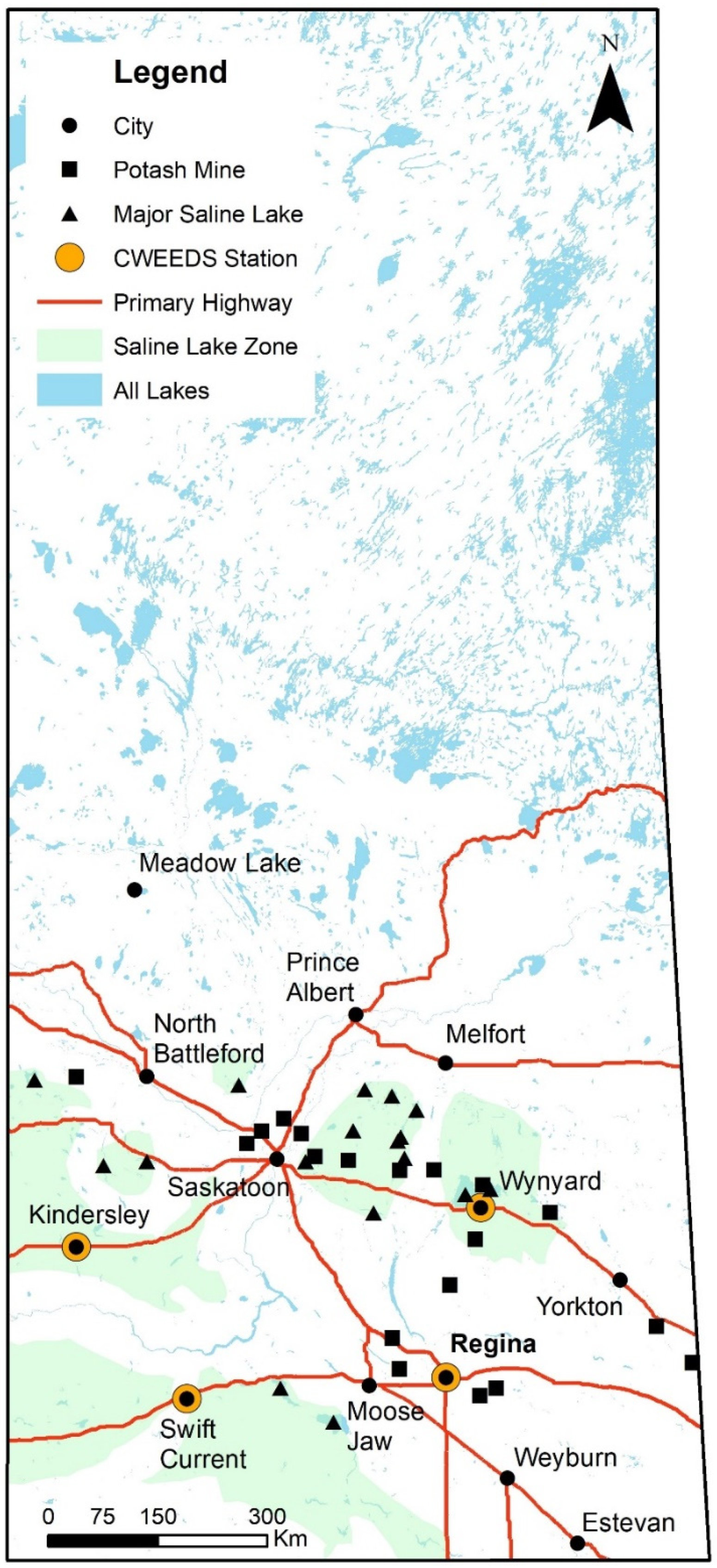
Figure 1 shows the geographical distribution of freshwater lakes (with less than 0.5 g·L−1 dissolved salts) and saline lakes (with at least 3.0 g·L−1 dissolved salts) in Saskatchewan, Canada. Derived from the Wisconsinan Glaciation (2.5 × 10⁶ to 17,000 years B.P.), the terrain is flat and undulating with the last melt of the Laurentide ice sheet (from 17,000 to 8000 years B.P), creating thousands of freshwater lakes with shallow depths and large exposed areas [20]. Likewise, there are approximately 500 saline lakes of at least 1 km2 areas [1], with high concentrations of dissolved salt [21]. These salts originate from the dissolution of ions as groundwater moved through geologic formations [22]. Alternating carbonate and evaporite formations have led to the development of lean and shallow aquifers (3 g·L−1 salts comprising Na+, Ca2+, Mg2+, and SO42−), as well as concentrated and deep aquifers (300 g·L−1 salts of Na+ and Cl−) [2]. Furthermore, several potash tailing ponds exist in the area containing slimes with dissolved salt contents of up to 360 g·L−1 [19]. In addition, the area is undergoing extensive changes due to the development of an irrigation system with a significant impact on agricultural practices. To ensure sustainable water use in the region (freshwater bodies, saline lakes, and tailings ponds), there is an exigent need to understand the effect of salinity on water evaporation under the prevalent climate.
The main objective of this research was to investigate the effect of salinity on evaporation using laboratory bench-scale testing. The evaporative fluxes from distilled water and saturated brine were measured under the imposed surface and atmospheric conditions representative of the Canadian Prairies. The two data sets were cross-examined and compared with predictions from established empirical equations.
2. Research Methodology
Evaporative flux tests were conducted using a bench-scale atmosphere simulator developed by Suchan and Azam [23], which replicated six different environmental scenarios in the study area. Table 1 provides the average atmospheric and surface parameters for the selected scenarios (spring, summer, and fall), showing both daytime and nighttime values. Winter was not included because freezing conditions are prevalent during this season. The atmospheric parameters (hourly land-based measurements) were obtained from the Canadian Weather Energy and Engineering Datasets (CWEEDS), based on data from 1998 to 2014. Details on the selection of surface–atmosphere parameters and standard deviations are given in Suchan and Azam [24].
The tests were conducted using 15 mL of sample (distilled water and saturated brine) in a clean and air-dried container mounted on an analytical scale balance. The freshwater stock was composed of distilled water containing less than 0.3 g·L−1 of dissolved salts. A saturated hypersaline brine stock was prepared by adding 100 mL of distilled water with 35.7 g of NaCl (TDS of 357 g·L−1) and stirring until all the solids were completely dissolved. The evaporative flux tests with water were conducted for approximately 3 h similar to İnan and Özgür [25], whereas the brine tests were conducted for approximately 6 h to account for the anticipated reduction in evaporation rate [26]. This generated approximately 1100 measurements for the distilled water and approximately 2200 measurements for the saturated brine at 10 s intervals. The average evaporative flux over the course of each experiment was determined using the change in sample mass over time and the surface area of the sample.
3. Results and Discussion
Table 2 provides a summary of the measured average atmospheric conditions and surface parameters for distilled water and saturated brine tests for the investigated weather scenarios. All of the target weather conditions (air velocity, air pressure, relative humidity, air temperature, and incoming solar irradiance) were achieved. The outgoing shortwave flux was similar between fluids and was found to not exceed 2 W m−2 (1% of incoming solar irradiance). This is primarily attributed to the stationary and perpendicular flux source in the atmospheric simulator that does not capture the moving and angular direction of the sun [27] or the effects of latitude [28]. The rate of mass change due to evaporation was obtained from the best fit to measured data (not given in this paper). The resulting values were found to range between 0.9 × 10⁻⁴ g∙s−1 and 2.8 × 10⁻⁴ g∙s−1. Finally, the surface temperature was achieved for each weather scenario, thereby capturing the long-term heat storage in deep water bodies [29].
Table 3 gives a summary of the analyzed data of average atmospheric and surface parameters for the investigated weather scenarios. The corresponding transient data (not given in this paper) were found to be steady. The aerodynamic resistance was found to be inversely related to air velocity and ranged from 41 s∙m−1 to 47 s∙m−1. Likewise, the absolute humidity was represented by the lower-upwind hygrometer, and the target results were achieved in the setup. The vapor pressure deficits (atmospheric and surface) were nearly the same for water and brine surfaces because the analyzed values are based on the controlled parameters of humidity, air temperature, and surface temperature. The atmospheric vapor pressure deficit followed the air temperature trends with high diurnal variation in summer (989 Pa and 938 Pa) and negligible variation in spring (83 Pa and 81 Pa) and fall (67 Pa and 69 Pa); values in parentheses are for water and brine, respectively. Similarly, the surface vapor pressure deficit followed the surface temperature trends, with high diurnal variation in summer (685 Pa and 606 Pa) and spring (468 Pa and 438 Pa) and low variation in fall (−256 Pa and −252 Pa).
The determination of energy fluxes was based on an infinitely thin surface with no heat storage [30], such that inputs and outputs were categorized as either radiant, evaporative, sensible, or ground flux, with details provided by Suchan and Azam [24]. The available energy (difference between net radiant flux and ground flux) at the water surface was generally twice that at the brine surface because the presence of salt decreases fluid chemical potential, thereby reducing the latent heat energy of the brines [5]. The diurnal pattern of the available energy was found to be similar to surface vapor pressure deficit, namely: high variation in the spring (359 J·s−1·m−2 and 194 J·s−1·m−2) and summer (179 J·s−1·m−2 and 195 J·s−1·m−2), and low in the fall (−90 J·s−1·m−2 and −72 J·s−1·m−2); values presented in parentheses are for water and brine, respectively.
Evaporative flux was obtained from the measured rate of change in mass and the surface area. The data followed seasonal patterns similar to the surface vapor pressure deficit and the available energy, namely large diurnal variation during spring (839 × 10−4 g·s−1·m−2 and 534 × 10−4 g·s−1·m−2) and summer (797 × 10−4 g·s−1·m−2 and 793 × 10−4 g·s−1·m−2), and small variation in the fall (−199 × 10−4 g·s−1·m−2 and −133 × 10−4 g·s−1·m−2); values presented in parentheses are for water and brine, respectively.
Figure 2 presents the results of the bench-scale testing in the form of evaporation rate with respect to time. As expected, the water loss from distilled water exceeded brine for all of the investigated weather scenarios. The evaporative flux from water surfaces was found to be stable, with data scatter (standard deviation) of 45–64 × 10−4 g·s−1·m−2 during the day and 23–27 × 10−4 g·s−1·m−2 at night. With the exception of summer day and fall night, a similarly stable flux was observed from brine surfaces with data scatter of 35–45 × 10−4 g·s−1·m−2 during the day and 6–57 × 10−4 g·s−1·m−2 at night. The evaporative flux gradually increased for brine surfaces during summer day (±162 × 10−4 g·s−1·m−2) and fall night (±94 × 10−4 g·s−1·m−2) and is attributed to the formation of NaCl crystals. The lower emissivity of solid crystals (ε = 0.87) compared with that of brine fluid (ε = 0.96) interfered with the infrared thermometer, thereby resulting in lower surface temperature readings [31]. These lower readings caused a gradual temperature increase in the silicon heating pad, thereby inadvertently increasing evaporative flux. In each weather scenario, the rate of evaporation from saturated brine surfaces is typically half the distilled water value. In the spring and summer, evaporation is twice as high during the day as compared to night for distilled water and three times higher for brine. Conversely, in the fall scenario, evaporative fluxes for both water and brine are approximately the same during the day and night.
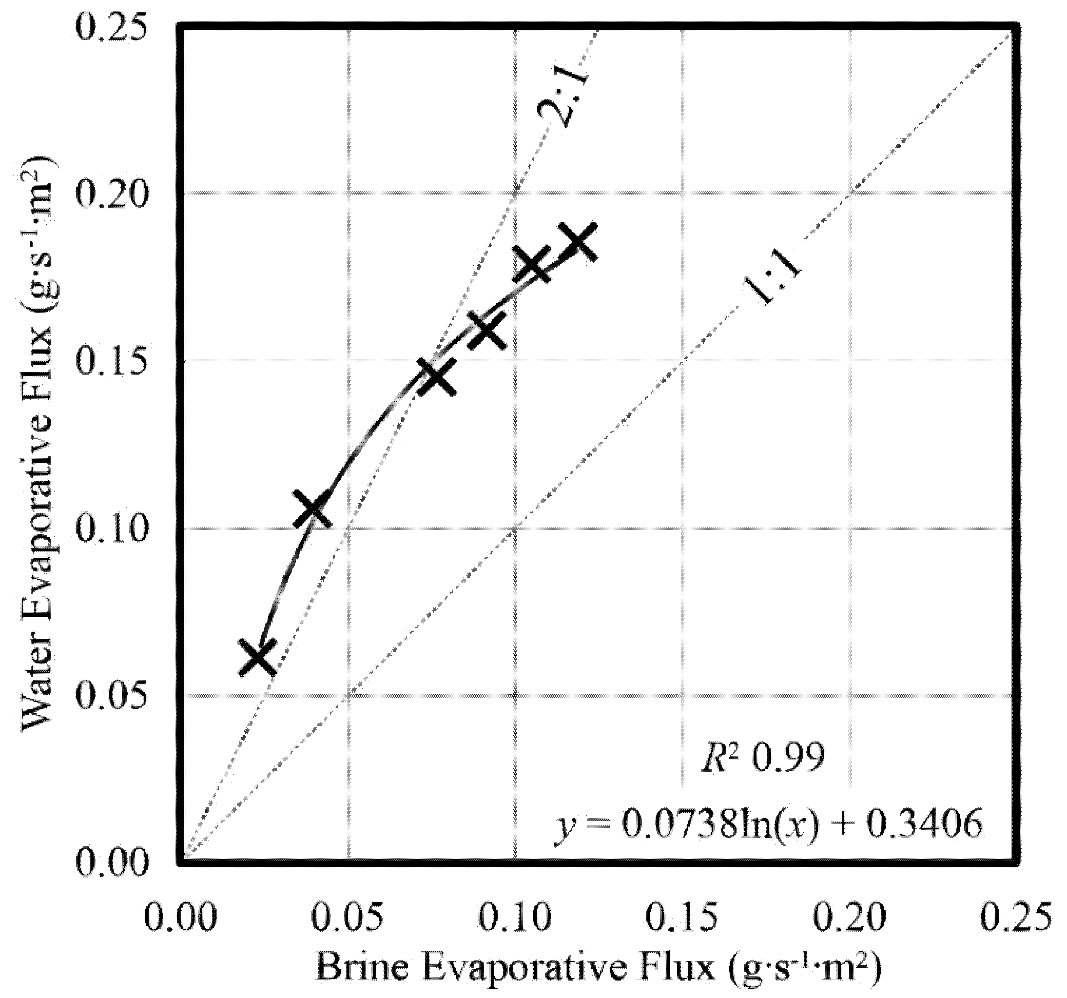
Figure 3 compares evaporative flux from distilled water and saturated brine surfaces. For the investigated range of surface-atmosphere conditions, the evaporative water flux was more than double that of brine (that is, 2:1 relationship) following a logarithmic equation (R2 = 0.99). This relationship, along with the associated scatter in data, is primarily related to the effect of NaCl on the measurement of the various parameters during testing.
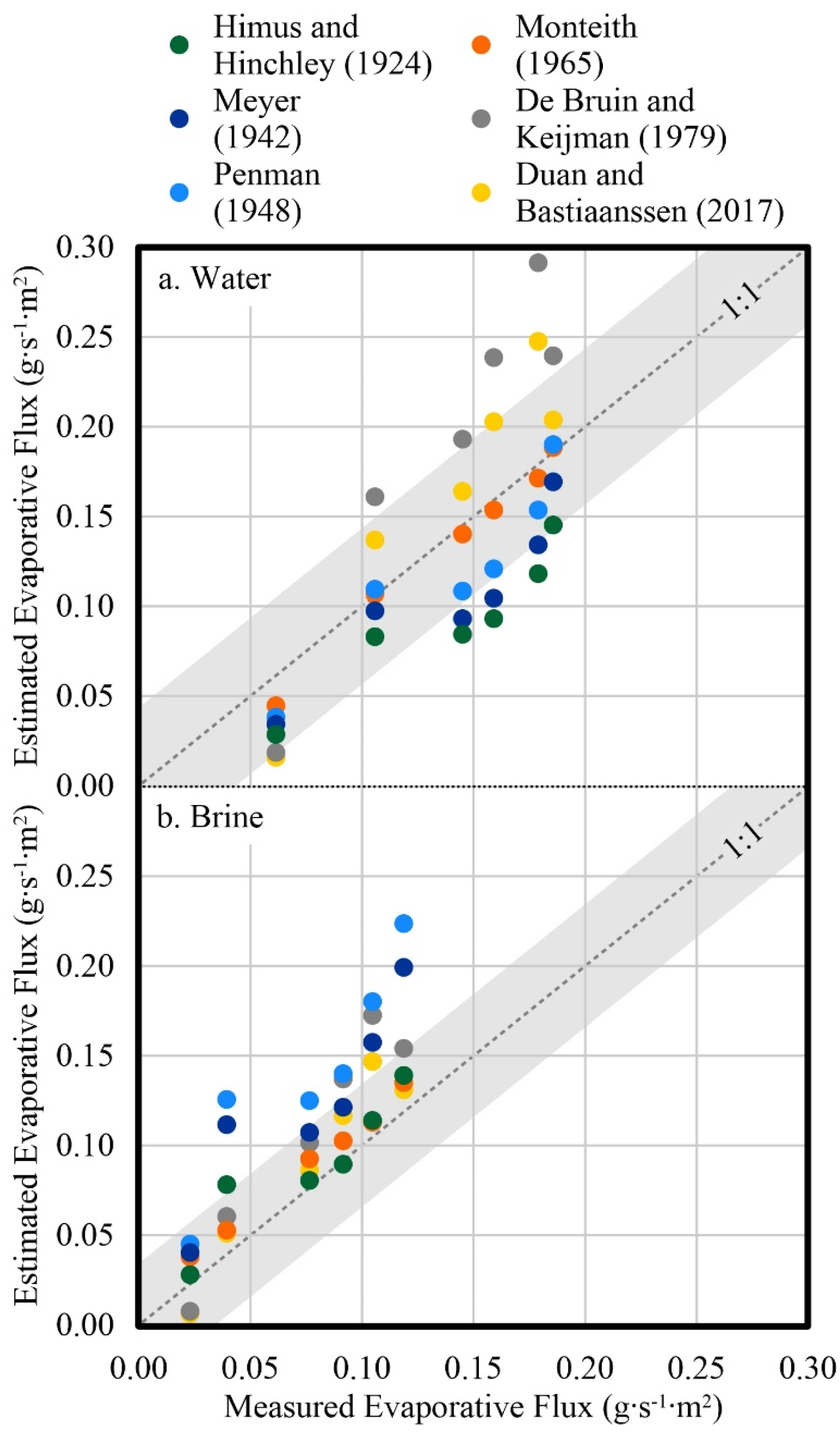
Figure 4 compares the measured evaporative flux values with estimates based on empirical relationships relevant to measured data. Table 4 provides a summary of the mass transfer equations such as Himus and Hinchley [32], Meyer [33], and Penman [34] and the combination equations by Monteith [35], De Bruin and Keijman [36], and Duan and Bastiaanssen [37]. The equations are modified to estimate evaporation from saturated brines, under the assumption that dissolved salt reduces the saturation vapor pressure by lowering the activity [5], and can be accommodated in mathematical equations using the concentration of sodium chloride () to determine the water activity coefficient [38]:
For distilled water (Figure 4a), the data are plotted on both sides of the equality line and mostly within one standard deviation of the water data. In contrast, the saturated brine (Figure 4b) is exclusively plotted above the equality line and mostly within one standard deviation of the brine data.
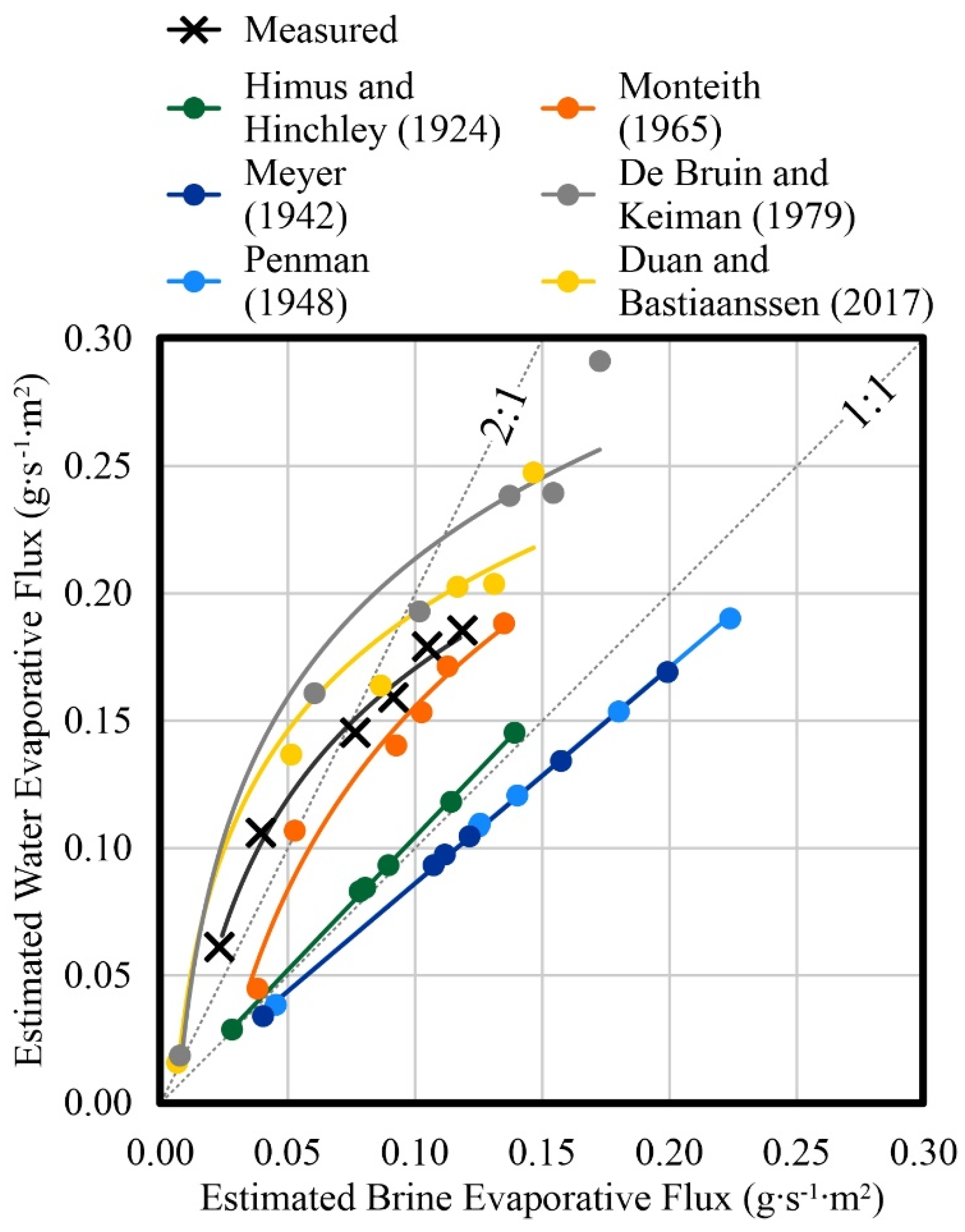
Figure 5 and Table 5 compare the estimated evaporative flux values of distilled water and saturated brine for the above-mentioned equations. The mass transfer models were best fitted with linear regressions that remained close to the 1:1 line (R2 = 0.99 and TSS = 1 × 10⁻²) because only measured parameters of air velocity and atmospheric vapor pressure deficit are taken into consideration. The trend lines for the Penman and the Meyer equations were found to overlap. All these equations included unique fit parameters that were calculated based on measured data. In contrast, the combination models were best fitted with logarithmic regressions that remained close to the 2:1 line (R2 ranging from 0.96 to 0.98, and TSS from 1 × 10⁻² to 5 × 10⁻²), attributed to the inclusion of surface vapor pressure, latent heat, and available energy parameters. These models, which took both mass and energy flux into account, were found to be closer to measured data and captured the logarithmic trend.
4. Summary and Conclusions
A thorough comprehension of evaporative flux from water and brine surfaces in semi-arid climates is necessary to estimate water losses. Laboratory evaporation tests on distilled water and saturated brine were conducted using a custom-built bench-scale atmospheric simulator with climatic parameters and surface conditions representative of the Canadian Prairies. The main conclusions of this study are given as follows:
The test results using a bench-scale atmosphere simulator indicated that the evaporative flux had a large variation during spring (water/brine: 1452/764 × 10−4 g·s−1·m−2 day and 613/230 × 10−4 g·s−1·m−2 night) and summer (1856/1187 × 10−4 g·s−1·m−2 day and 1059/394 × 10−4 g·s−1·m−2 night), and small variation in the fall (1591/915 × 10−4 g·s−1·m−2 day and 1790/1048 × 10−4 g·s−1·m−2 night).
The primary theoretical contribution of this research is that the evaporation rate from the distilled water surface is twice that of the saturated brine surface. The measured data for water correlated well with mathematical estimates; data scatter was evenly distributed and within one standard deviation of the equality line, whereas the brine data mostly plotted above the equality line.
The newly developed 2:1 correlation between evaporation rates from water surfaces versus brine surfaces was found to follow the trend lines of the combination equations, and the Monteith model best matched the measure data. In contrast, the mass transfer models were best fitted with linear regressions that remained close to the 1:1 line for water and brine evaporation.
Author Contributions
Data curation and analysis, J.S.; Supervision, S.A.; Writing—original draft, J.S.; Writing—review and editing, S.A. All authors have read and agreed to the published version of the manuscript.
Funding
Natural Science and Engineering Research Council of Canada.
Institutional Review Board Statement
Not applicable.
Informed Consent Statement
Not applicable.
Data Availability Statement
The authors can provide access to test data upon request.
Acknowledgments
The authors would like to thank the University of Regina for providing laboratory space.
Conflicts of Interest
The authors declare there is no conflict of interest.
References
- Hammer, U.T. Saline lake resources of the Canadian Prairies. Can. Water Resour. J. 1986, 11, 43–57. [Google Scholar] [CrossRef] [Green Version]
- Last, W.M.; Slezak, L.A. The salt lakes of western Canada: A paleolimnological overview. Hydrobiologia 1988, 158, 301–316. [Google Scholar] [CrossRef]
- Salhotra, A.M.; Adams, E.E.; Harleman, D.R.F. Effect of salinity and ionic composition on evaporation: Analysis of Dead Sea evaporation pans. Water Resour. Res. 1985, 21, 1336–1344. [Google Scholar] [CrossRef]
- Finch, J.W.; Calver, A. Methods for the Quantification of Evaporation from Lakes; Centre for Ecology & Hydrology: Oxfordshire, UK, 2008. [Google Scholar]
- Akridge, D.G. Methods for calculating brine evaporation rates during salt production. J. Archaeol. Sci. 2008, 35, 1453–1462. [Google Scholar] [CrossRef]
- Schulz, S.; Darehshouri, S.; Hassanzadeh, E.; Tajrishy, M.; Schüth, C. Climate change or irrigated agriculture—What drives the water level decline of Lake Urmia. Sci. Rep. 2020, 10, 236. [Google Scholar] [CrossRef] [PubMed] [Green Version]
- Trautz, A.C.; Illangasekare, T.H.; Howington, S. Experimental testing scale considerations for the investigation of bare-soil evaporation dynamics in the presence of sustained above-ground airflow. Water Resour. Res. 2018, 54, 8963–8982. [Google Scholar] [CrossRef]
- Lemmen, D.S.; Vance, R.E.; Campbell, I.A.; David, P.P.; Pennock, D.J.; Sauchyn, D.J.; Wolfe, S.A. Geomorphic Systems of the Palliser Triangle, Southern Canadian Prairies: Description and Response to Changing Climate; Natural Resources Canada: Ottawa, ON, Canada, 1998. [Google Scholar]
- Faurès, J.M.; Hoogeveen, J.; Winpenny, J.; Steduto, P.; Burke, J. Coping with Water Scarcity: An Action Framework for Agriculture and Food Security; Food and Agriculture Organization of the United Nations: Rome, Italy, 2012. [Google Scholar]
- Akhter, A.; Azam, S. Flood-drought hazard assessment for a flat clayey deposit in the Canadian Prairies. J. Environ. Inform. Lett. 2019, 1, 8–19. [Google Scholar] [CrossRef]
- Fang, X.; Pomeroy, J.W. Drought impacts on Canadian prairie wetland snow hydrology. Hydrol. Process. 2008, 22, 2858–2873. [Google Scholar] [CrossRef]
- Cutlac, I.; Horbulyk, T.M. Optimal water allocation under short-run water scarcity in the South Saskatchewan River Basin. J. Water Resour. Plan. Manag. 2011, 137, 92–100. [Google Scholar] [CrossRef]
- Wheater, H.; Gober, P. Water security in the Canadian Prairies: Science and management challenges. Philos. Trans. Math. Phys. Eng. Sci. 2013, 371, 1–21. [Google Scholar] [CrossRef]
- Pomeroy, J.W.; Shook, K.R. Review of Lake Diefenbaker Operations 2010–2011; Centre for Hydrology, University of Saskatchewan: Saskatoon, SK, Canada, 2012. [Google Scholar]
- Hammer, U.T. The saline lakes of Saskatchewan, I. Background and rationale for saline lakes research. Int. Rev. Gesamten Hydrobiol. Hydrogr. 1978, 63, 173–177. [Google Scholar] [CrossRef]
- Bowman, J.S.; Sachs, J.P. Chemical and physical properties of some saline lakes in Alberta and Saskatchewan. Saline Syst. 2008, 4, 3. [Google Scholar] [CrossRef] [PubMed] [Green Version]
- Tallin, J.E.; Pufahl, D.E.; Barbour, S.L. Waste management schemes of potash mines in Saskatchewan. Can. J. Civil. Eng. 1990, 17, 528–542. [Google Scholar] [CrossRef]
- Reid, K.W. Water use in Saskatchewan’s potash industry and opportunities for water recycling/conservation. Can. Water Resour. J. 1984, 9, 21–26. [Google Scholar] [CrossRef]
- Landine, P. Weathering and Diagenesis of Saskatchewan Potash Tailings; University of Saskatchewan: Saskatoon, SK, Canada, 1993. [Google Scholar]
- Christiansen, E.A. The Wisconsinan deglaciation, of southern Saskatchewan and adjacent areas. Can. J. Earth Sci. 1979, 16, 913–938. [Google Scholar] [CrossRef]
- Last, W.M.; Ginn, F.M. Saline systems of the Great Plains of western Canada: An overview of the limnogeology and paleolimnology. Saline Syst. 2005, 1, 10. [Google Scholar] [CrossRef] [Green Version]
- Bredehoeft, J.D.; Blyth, C.R.; White, W.A.; Maxey, G.B. Possible mechanism for concentration of brines in subsurface formations. Bull. Am. Assoc. Pet. Geol. 1963, 47, 257–269. [Google Scholar]
- Suchan, J.; Azam, S. Development of BAS2 for determination of evaporative fluxes. MethodsX 2021, 8, 101424. [Google Scholar] [CrossRef]
- Suchan, J.; Azam, S. Determination of Evaporative Fluxes Using a Bench-Scale Atmosphere Simulator. Water 2021, 13, 84. [Google Scholar] [CrossRef]
- İnan, M.; Özgür, S. Experimental investigation of evaporation from a horizontal free water surface. Sigma J. Eng. Nat. Sci. 2017, 35, 119–131. [Google Scholar]
- Mor, Z.; Assouline, S.; Tanny, J.; Lensky, I.M.; Lensky, N.G. Effect of water surface salinity on evaporation: The case of a diluted buoyant plume over the Dead Sea. Water Resour. Res. 2018, 54, 1460–1475. [Google Scholar] [CrossRef]
- Patel, S.S.; Rix, A.J. The impact of water surface albedo on incident solar insolation of a collector surface. In Proceedings of the 2020 International SAUPEC/RobMech/PRASA Conference, Cape Town, South Africa, 29–31 January 2020; pp. 1–6. [Google Scholar]
- Shuttleworth, W.J. Evaporation. In Handbook of Hydrology; Maidment, D.R., Ed.; McGraw-Hill Inc.: New York, NY, USA, 1993; pp. 4.1–4.53. [Google Scholar]
- Finch, J.W. A comparison between measured and modelled open water evaporation from a reservoir in south-east England. Hydrol. Process. 2001, 15, 2771–2778. [Google Scholar] [CrossRef]
- Granger, R.J.; Gray, D.M. Evaporation from natural nonsaturated surfaces. J. Hydrol. 1989, 111, 21–29. [Google Scholar] [CrossRef]
- Vázquez, O.; Thomachot-Schneider, C.; Mouhoubi, K.; Gommeaux, M.; Fronteau, G.; Barbin, V.; Bodnar, J. Study of NaCl crystallization with passive infrared thermography. In Proceedings of the SWBSS 3rd International Conference on Salt Weathering of Buildings and Stone Sculptures, Brussels, Belgium, 14–16 October 2014. [Google Scholar]
- Himus, G.W.; Hinchley, J.W. The effect of a current of air on the rate of evaporation of water below the boiling point. J. Soc. Chem. Ind. 1924, 43, 840–845. [Google Scholar] [CrossRef]
- Meyer, A.F. Evaporation from Lakes and Reservoirs; Minnesota Resources Commission: St. Paul, MN, USA, 1942. [Google Scholar]
- Penman, H.L. Natural evaporation from open water, bare soil and grass. Proc. R. Soc. Lond. 1948, 193, 120–145. [Google Scholar]
- Monteith, J.L. Evaporation and environment. Symp. Soc. Exp. Biol. 1965, 19, 205–234. [Google Scholar] [PubMed]
- De Bruin, H.; Keijman, J.Q. The Priestley-Taylor evaporation model applied to a large, shallow lake in the Netherlands. J. Appl. Meteorol. 1979, 18, 898–903. [Google Scholar] [CrossRef] [Green Version]
- Duan, Z.; Bastiaanssen, W.G.M. Evaluation of three energy balance-based evaporation models for estimating monthly evaporation for five lakes using derived heat storage changes from a hysteresis model. Environ. Res. Lett. 2017, 12, 024005. [Google Scholar] [CrossRef] [Green Version]
- Lide, D.R. CRC Handbook of Chemistry and Physics; CRC Press, Taylor & Francis Group: Boca Raton, FL, USA; London, UK; New York, NY, USA, 2004. [Google Scholar]
Figure 1.
Geographical distribution of freshwater lakes, saline lakes, and potash mines in Saskatchewan, Canada.
Figure 1.
Geographical distribution of freshwater lakes, saline lakes, and potash mines in Saskatchewan, Canada.

Figure 2.
Evaporative flux in the study area for distilled water and saturated brine in (a) spring day, (b) summer day, (c) fall day, (d) spring night, (e) summer night, and (f) fall night.
Figure 2.
Evaporative flux in the study area for distilled water and saturated brine in (a) spring day, (b) summer day, (c) fall day, (d) spring night, (e) summer night, and (f) fall night.

Figure 3.
Measured evaporative flux correlation between distilled water and saturated brine surfaces.
Figure 3.
Measured evaporative flux correlation between distilled water and saturated brine surfaces.

Figure 4.
Comparison of estimated and measured evaporative flux for (a) distilled water and (b) saturated brine.
Figure 4.
Comparison of estimated and measured evaporative flux for (a) distilled water and (b) saturated brine.

Figure 5.
Comparison of evaporative fluxes from distilled water and saturated brine surfaces using various methods.
Figure 5.
Comparison of evaporative fluxes from distilled water and saturated brine surfaces using various methods.


Table 1.
Selected atmospheric parameters in the study area, modified after Suchan and Azam [24].
Table 1.
Selected atmospheric parameters in the study area, modified after Suchan and Azam [24].
| Weather Scenario | Date Range (Month) | Duration (Hours) | Air Velocity (m∙s−1) | Air Humidity (g∙m−3) | Air Temperature (°C) | Solar Irradiance (W∙m−2) | Surface Temperature (°C) |
|---|---|---|---|---|---|---|---|
| Day | March–November | 3706 | |||||
| Spring | March–May | 883 | 1.7 | 5.0 | 10.0 | 325 | 12 |
| Summer | May–September | 1755 | 1.3 | 9.0 | 19.0 | 325 | 22 |
| Fall | September–November | 541 | 1.6 | 5.0 | 9.0 | 210 | 13 |
| Night | April–November | 1827 | |||||
| Spring | April–May | 206 | 1.3 | 5.0 | 9.0 | 0 | 6 |
| Summer | May–September | 761 | 1.3 | 8.5 | 13.0 | 0 | 17 |
| Fall | September–November | 277 | 1.5 | 5.5 | 9.0 | 0 | 16 |
Table 2.
Summary of the measured average atmospheric and surface parameters.
| Parameter | Unit | Symbol | ||||||||||||
|---|---|---|---|---|---|---|---|---|---|---|---|---|---|---|
| Day | Night | |||||||||||||
| Spring | Summer | Fall | Spring | Summer | Fall | |||||||||
| W | B | W | B | W | B | W | B | W | B | W | B | |||
| Count | n | 1102 | 1988 | 1236 | 2161 | 1184 | 2161 | 1250 | 2158 | 1084 | 1777 | 1232 | 2161 | |
| Atmosphere | ||||||||||||||
| Momentum | ||||||||||||||
| Velocity | m∙s−1 | 1.7 | 1.7 | 1.3 | 1.3 | 1.6 | 1.6 | 1.3 | 1.3 | 1.3 | 1.3 | 1.5 | 1.5 | |
| Mass | ||||||||||||||
| Air Pressure | Pa | 94,294 | 95,893 | 95,397 | 95,134 | 93,414 | 95,293 | 94,484 | 95,845 | 94,407 | 93,256 | 95,060 | 92,866 | |
| Relative Humidity | ||||||||||||||
| Upwind, High | % | 50.8 | 50.7 | 51.3 | 52.0 | 55.1 | 53.9 | 54.4 | 54.5 | 75.2 | 76.0 | 60.7 | 64.8 | |
| Downwind, High | % | 53.5 | 53.0 | 51.9 | 52.9 | 57.5 | 56.4 | 55.5 | 55.7 | 80.5 | 76.6 | 61.2 | 66.1 | |
| Upwind, Low | % | 52.7 | 53.2 | 55.0 | 55.3 | 56.5 | 56.4 | 56.6 | 56.7 | 75.1 | 74.9 | 62.3 | 62.2 | |
| Downwind, Low | % | 55.7 | 56.2 | 57.6 | 57.8 | 59.9 | 59.6 | 59.5 | 59.5 | 80.5 | 80.3 | 66.2 | 68.4 | |
| Energy | ||||||||||||||
| Temperature | ||||||||||||||
| Upwind, High | °C | 10.8 | 11.0 | 20.7 | 20.5 | 9.5 | 9.8 | 9.7 | 9.6 | 13.7 | 13.7 | 9.7 | 9.4 | |
| Downwind, High | °C | 10.3 | 10.5 | 20.4 | 20.2 | 9.0 | 9.3 | 9.5 | 9.4 | 13.0 | 13.6 | 9.4 | 9.1 | |
| Upwind, Low | °C | 10.1 | 10.1 | 19.0 | 19.0 | 8.9 | 9.1 | 9.1 | 8.9 | 12.9 | 13.1 | 8.9 | 9.0 | |
| Downwind, Low | °C | 9.9 | 10.0 | 19.2 | 19.1 | 8.8 | 9.0 | 9.0 | 8.9 | 13.0 | 13.1 | 8.9 | 9.0 | |
| Shortwave Flux (↓) | W∙m−2 | 325 | 325 | 325 | 325 | 210 | 210 | 0 | 0 | 0 | 0 | 0 | 0 | |
| Surface | ||||||||||||||
| Mass | ||||||||||||||
| Mass Rate Change (× 10−4) | g∙s−1 | 2.17 | 1.12 | 2.79 | 1.72 | 2.39 | 1.34 | 0.93 | 0.34 | 1.60 | 0.59 | 2.68 | 1.54 | |
| Energy | ||||||||||||||
| Shortwave Flux (↑) | W∙m−2 | 2 | 2 | 2 | 2 | 1 | 2 | 0 | 0 | 0 | 0 | 0 | 0 | |
| Temperature | °C | 12 | 12 | 22 | 22 | 13 | 13 | 6 | 6 | 17 | 17 | 16 | 16 | |
Note. Surface materials are distilled water (W) and saturated brine (B).
Table 3.
Summary of the analyzed average atmospheric and surface parameters.
| Parameter | Unit | Symbol | ||||||||||||
|---|---|---|---|---|---|---|---|---|---|---|---|---|---|---|
| Day | Night | |||||||||||||
| Spring | Summer | Fall | Spring | Summer | Fall | |||||||||
| W | B | W | B | W | B | W | B | W | B | W | B | |||
| Atmosphere | ||||||||||||||
| Momentum | ||||||||||||||
| Aero. Resistance | s∙m−1 | 41.4 | 41.4 | 46.6 | 46.8 | 42.6 | 42.6 | 46.6 | 46.6 | 46.6 | 46.6 | 43.9 | 43.9 | |
| Mass | ||||||||||||||
| Vapor Density | g∙m−3 | 5.0 | 5.0 | 9.0 | 9.0 | 5.0 | 5.0 | 5.0 | 5.0 | 8.5 | 8.5 | 5.5 | 5.5 | |
| Vapor Pressure | ||||||||||||||
| Partial | Pa | 650 | 658 | 1209 | 1215 | 646 | 651 | 652 | 648 | 1117 | 1126 | 712 | 715 | |
| Saturated | Pa | 1234 | 1211 | 2198 | 2152 | 1144 | 1131 | 1153 | 1121 | 1488 | 1473 | 1144 | 1125 | |
| Deficit | Pa | 584 | 554 | 989 | 938 | 498 | 480 | 501 | 473 | 371 | 347 | 431 | 411 | |
| Energy | ||||||||||||||
| Longwave Flux (↓) | J∙s−1∙m−2 | 284 | 284 | 340 | 340 | 279 | 280 | 280 | 280 | 313 | 314 | 282 | 283 | |
| Surface | ||||||||||||||
| Mass | ||||||||||||||
| Vapor Pressure | ||||||||||||||
| Saturated | Pa | 1402 | 1375 | 2646 | 2593 | 1498 | 1468 | 936 | 927 | 1938 | 1899 | 1820 | 1784 | |
| Deficit | Pa | 752 | 717 | 1437 | 1379 | 852 | 817 | 284 | 279 | 821 | 773 | 1108 | 1069 | |
| Energy | ||||||||||||||
| Longwave Flux (↑) | J∙s−1∙m−2 | 367 | 367 | 422 | 422 | 373 | 373 | 337 | 338 | 394 | 394 | 389 | 388 | |
| Net Radiant Heat Flux | J∙s−1∙m−2 | 241 | 241 | 241 | 242 | 117 | 118 | −58 | −59 | −80 | −79 | −107 | −106 | |
| Evaporative Heat Flux | J∙s−1∙m−2 | 359 | 189 | 464 | 291 | 398 | 226 | 160 | 57 | 258 | 97 | 432 | 258 | |
| Sensible Heat Flux | J∙s−1∙m−2 | 46 | 24 | 47 | 29 | 112 | 60 | −114 | −39 | 74 | 28 | 167 | 100 | |
| Ground Heat Flux | J∙s−1∙m−2 | −164 | 28 | −270 | −78 | −393 | −168 | −104 | −77 | −412 | −204 | −706 | −464 | |
| Available Energy | J∙s−1∙m−2 | 405 | 213 | 511 | 320 | 509 | 286 | 46 | 19 | 332 | 125 | 599 | 358 | |
| Evaporative Flux (×10−4) | J∙s−1∙m−2 | 1452 | 764 | 1856 | 1187 | 1591 | 915 | 613 | 230 | 1059 | 394 | 1790 | 1048 | |
Note. Surface materials are distilled water (W) and saturated brine (B).
Table 4.
Summary of empirical equations for estimation of evaporative flux, modified after Suchan and Azam [24].
Table 4.
Summary of empirical equations for estimation of evaporative flux, modified after Suchan and Azam [24].
| Type and Reference | Vapor Flux Equation (g∙m−2∙s−1) |
|---|---|
| Mass-Transfer | |
| [32] | |
| [33] | |
| [34] | |
| Combination | |
| [35] | |
| [36] | |
| [37] |
Table 5.
Comparative statistical summary of evaporative fluxes from distilled water and saturated brine surfaces using various methods.
Table 5.
Comparative statistical summary of evaporative fluxes from distilled water and saturated brine surfaces using various methods.
| Method | Best Fit | Coefficient of Determination (R2) | Residual Sum of Squares (SSE) | Regression Sum of Squares (SSR) | Total Sum of Squares (TSS) |
|---|---|---|---|---|---|
| BAS2 | Logarithmic | 0.9910 | 1 × 10⁻⁴ | 0.0112 | 0.0113 |
| [32] | Linear | 0.9997 | 3 × 10⁻⁶ | 0.0080 | 0.0080 |
| [33] | Linear | 0.9994 | 6 × 10⁻⁶ | 0.0102 | 0.0102 |
| [34] | Linear | 0.9997 | 8 × 10⁻⁶ | 0.0129 | 0.0129 |
| [35] | Logarithmic | 0.9616 | 5 × 10⁻⁴ | 0.0129 | 0.0134 |
| [36] | Logarithmic | 0.9778 | 2 × 10⁻³ | 0.0433 | 0.0453 |
| [37] | Logarithmic | 0.9559 | 1 × 10⁻³ | 0.0313 | 0.0327 |
Publisher’s Note: MDPI stays neutral with regard to jurisdictional claims in published maps and institutional affiliations. |
© 2021 by the authors. Licensee MDPI, Basel, Switzerland. This article is an open access article distributed under the terms and conditions of the Creative Commons Attribution (CC BY) license (https://creativecommons.org/licenses/by/4.0/).
Share and Cite
MDPI and ACS Style
Suchan, J.; Azam, S. Effect of Salinity on Evaporation from Water Surface in Bench-Scale Testing. Water 2021, 13, 2067. https://doi.org/10.3390/w13152067
AMA Style
Suchan J, Azam S. Effect of Salinity on Evaporation from Water Surface in Bench-Scale Testing. Water. 2021; 13(15):2067. https://doi.org/10.3390/w13152067
Chicago/Turabian StyleSuchan, Jared, and Shahid Azam. 2021. "Effect of Salinity on Evaporation from Water Surface in Bench-Scale Testing" Water 13, no. 15: 2067. https://doi.org/10.3390/w13152067
Note that from the first issue of 2016, this journal uses article numbers instead of page numbers. See further details here.