
Study on the Comprehensive Improvement of Ecosystem Services in a China’s Bay City for Spatial Optimization

1
School of Resource and Environmental Sciences, Wuhan University, Wuhan 430079, China
2
College of Resources and Environmental Sciences, Henan Agricultural University, Zhengzhou 450002, China
3
College of Land Management, Huazhong Agricultural University, Wuhan 430070, China
4
School of Economics and Management, China University of Geosciences, Wuhan 430074, China
5
College of Water Sciences, Beijing Normal University, Beijing 100875, China
*
Authors to whom correspondence should be addressed.
Water 2021, 13(15), 2072; https://doi.org/10.3390/w13152072
Submission received: 16 June 2021
/
Revised: 26 July 2021
/
Accepted: 28 July 2021
/
Published: 29 July 2021
(This article belongs to the Special Issue Optimal Utilization and Management of Natural Resources)
Abstract
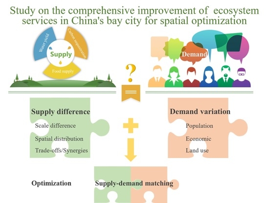
:Ecosystem services are characterized by region and scale, and contribute to human welfare. Taking Yantai city, a typical bay city in China, as the example, its three representative ecosystem services: food supply (FS), carbon sequestration (CS) and water yield (WY) were chosen as study targets. Based on analyzation of six different aspects of the supply and variation characteristic of demand, this study tried to propose advices for comprehensive improvement of ecosystem services for spatial optimization. The results showed that: (1) ecosystem services supply was strong in central and southern areas of Yantai, while the northern coastal areas were relatively weak; (2) synergistic relationships were found of FS-CS, FS-WY and CS-WY both in 2009 and 2015, with the strongest one for FS-WY. Additionally, in the synergistic relationships, each pair of ecosystem services was dominated by one ecosystem service; (3) most of the three pairs of synergistic relationships had the tendency to strengthen with larger scales; (4) four ecosystem demands changing areas were observed and comprehensive improvement suggestions for them were proposed. This work provides a new attempt to improve ecosystem services based on its supply-demand relationship, which will give a baseline reference for related studies in Yantai city, as well as other similar bay cities.
1. Introduction
Ecosystem services are the various direct or indirect benefits that people derive from ecosystems, including provisioning, regulating, cultural and supporting services, which are important links between ecosystems and human well-beings [1,2,3]. Influenced by the diversity of ecosystem services, the complexity of ecological processes and human preferences, different ecosystem services exhibit complex interactions, which can be described as trade-offs and synergies [4,5]. Trade-offs between multiple ecosystem services occur when the improvement of one ecosystem service is at the expense of the reduction of another ecosystem service. The trade-offs are common between provisioning services, and between provisioning and regulating services [6,7]. Conversely, the relationship is synergistic when an improvement in one ecosystem service leads to an increase in another [8]. The synergy is relatively common for regulating, supporting and cultural services [9,10]. In recent years, the contradiction between the excessive human demand for material and resources and the limited natural resources has become increasingly evident. Meeting the needs for food, water, materials and shelter for more than 7 billion people on the planet comes at the expense of natural ecosystems [11,12]. Rapid urbanization changes the land use pattern, which affects structures and processes of ecosystem and supply capacity of ecosystem services [13,14,15,16]. Increases in provisioning services are often accompanied by the sacrifice of other ecosystem services [17,18]. Ignorance of trade-offs/synergies may lead to the supply capacity decline of some ecosystem services and eventually even threaten the stability and security of the whole ecosystem [11]. Therefore, in order to maintain a healthy ecosystem and promote sustainable socio-economic development, it is important to understand the ecosystem services trade-offs/synergies and their spatial distribution characteristics to maximize human well-being.
Since the Millennium Ecosystem Assessment in 2001, the development of regional ecosystem service trade-offs/synergies and ecosystem management has become an important issue in ecosystem services research [19,20,21]. A great deal of exploration has also been carried out by scholars from around the world. The study involved ecosystems such as forests [22], agricultural lands [23], watersheds [24], grasslands [25], wetlands [26] and oceans [27]. The methods used in above studies included statistical methods [26,28], spatial analysis [29], scenario simulation [30,31] and model simulation [23,32]. Some scholars compared the methods in detail and found that the study of ecosystem services trade-offs still focused on qualitative or semi-quantitative analysis, and the spatial quantitative expression of trade-offs needed to be further strengthened [33]. Even though the research scales included global [34], continental [35], national [36,37], regional [32], city [23,38], rural [39,40] and landscape [41], there was a lack of multi-scale studies. The interactions between ecosystem services varied at both temporal and spatial scales, but the understanding of the spatiotemporal dynamics of ecosystem services trade-offs and synergies and related research is currently limited [42]. To effectively manage ecosystem services and keep their benefits for people [1,2,3,13], it is important to know how ecosystem services and their relationships changed in space and time. Ecosystem services interrelationships were driven by interactions between social and ecological variables [43]. However, the relative importance of the different social and biophysical drivers of ecosystem services and how these varied across socio-ecological systems was unclear, which was required further exploration. In addition, many studies used land-use data from remote sensing image interpretation, and few studies used data from national land-change surveys to focus on changes in ecosystem services [13,44,45]. Compared with the traditional interpretation data, land-change survey data can provide more detailed information [13,45]. Meanwhile, recently, growing attention has been paid to ecosystem service supply and demand mismatch [46,47,48]. Researchers tried to measure the changes in supply-demand of ecosystem services and the drivers [47,48,49,50,51,52,53,54]. Considerable progress was seen in the study of ecosystem services trade-offs, including trade-offs between any two ecosystem services [33,48,55] and trade-offs in supply-demand mismatch [48,51,56,57]. However, little study has considered to adjust and improve the ecosystem services combining the changes in the demand and the trade-offs/synergies in ecosystem services, using land-change survey data.
Bohai Rim is the gold coast of the northern coast of China, including three urban agglomerations (Beijing-Tianjin-Hebei, Central South Liaoning and Shandong Peninsula). Additionally, it is one of the three major economic growth poles in China. Since the implementation of China’s reform and opening-up policy and gathering of labor, capital, technology and other production factors, there has been a continuous improve of economic level and development of infrastructure construction in coastal areas. The Bohai Rim region has developed into the center of the North-East Asia Economic Circle. However, the Bohai Rim was faced with enormous environmental pressure, due to the irrational industrial structure and the extensive mode of economic development [58]. Currently, the amount of land-sourced pollutants entering the sea in the Bohai Rim has increased dramatically [59]. Marine and air pollution has worsened, and the natural coastline has shrunk sharply. The resources and environmental carrying capacity have been overloaded [60,61]. The contradiction between socio-economic development and ecological protection in the Bohai Rim area is becoming increasingly acute [60]. Urgent action is needed to achieve regional sustainable development. In recent years, many scholars have studied the ecosystem services and their changes [62], ecological risks [63] and ecological efficiency in Bohai Rim [64]. While using authoritative land-change survey data to analyze the spatiotemporal characteristics of trade-offs/synergies, scale effects, driving mechanisms and improvement of ecosystem services is lacked. Therefore, it is necessary to explore the spatial patterns of ecosystem services trade-offs and synergies, and propose some improvement suggestions in the context of rapid socio-economic development in Bohai Rim. Yantai City, a typical city in the Bohai Rim, was selected as the study area. Even though as a bay city, water shortage is always a big problem for it. Per capita water resource is lower than 500 m3 in over a half of the city. Meanwhile, carbon emission is large in the city because of large proportion of industrial production and mining. However, the city has relatively developed agricultural production, especially in fruits planting [65]. Thus, food supply, carbon sequestration and water yield were chosen as the representative ecosystem services in this study. Based on the land-change survey data, the spatiotemporal distribution characteristics of the three types of ecosystem services were analyzed. Through correlation analysis and the introduction of an ecosystem service trade-offs/synergies index, the spatiotemporal characteristics, scale effects and driving mechanisms of the trade-offs/synergies among the three types of ecosystem services were investigated. Meanwhile, on the basis of trade-offs/synergies and changes in ecosystem services demand, improvement suggestions of ecosystem services were proposed to provide decision support for ecosystem conservation and optimal management in Yantai and other bay city.
2. Materials and Methods
2.1. Study Area
Yantai is located in the eastern part of the Shandong Peninsula, China, and is an important port city in the Bohai Rim. The city governs 12 county-level administrative regions, with complex terrain conditions, as shown in Figure 1. The elevation is high in the middle of the territory, and low in the south and north, with the range of 0~922.8 m. The climate belongs to the warm temperate continental monsoon climate. It has an annual average temperature of 13.0 °C, a sunshine hour of 2611.6 h and an average annual precipitation of 680 mm. The precipitation is concentrated in summer (from June to September), accounting for more than 70% of the annual total precipitation. However, the spatial distribution of rainfall is uneven, which is significantly more in the central and southern hilly than the northern coastal areas. The water volume of rivers is greatly affected by rainfall, and drying-out of rivers are common to see during non-flood season. Water resources are extremely scarce in the city, with an average total water resources of only about 3.2 billion m3 over the years. Additionally, per-capita water resource is less than 500 m3, which is only one-fifth of the national average level. The lack of water resources has become an important limiting factor for future development. As the acceleration of urbanization, there are a large number of industrial zones, ports and docks under construction. Compared with other coastal cities, the proportion of industrial land in Yantai is relatively large, which has a greater negative impact on the environment. The urban ecological space has been drastically reduced, and environmental pollution has become more and more serious.
2.2. Data Sources
The land-change survey data in 2009 and 2015 was from Yantai Bureau of Land and Resources, including 8 primary types (arable land, garden plot, woodland, water area, construction land, grassland, traffic land and other land), and 33 sub-class types. The annual rainfall and Normalized Difference Vegetation Index (NDVI) data were obtained from the data center of resources and environment science, Chinese Academy of Sciences (http://www.resdc.cn/ (accessed on 1 August 2020)), with resolution of 1000 m× 1000 m. Evapotranspiration data was from MOD16 (http://www.ntsg.umt.edu/project/modis/mod16.php (accessed on 1 August 2020)), with resolution of 1000 m × 1000 m. Soil data were obtained from national soil survey data with resolution of 1000 m × 1000 m. Total water consumption and total population in 2009 and 2015 came from Shandong Yantai statistical yearbook (http://www.shujuku.org/shandong-statistical-yearbook.html (accessed on 1 August 2020)). The total output of grain, oil crops and vegetables, per capita food demand came from Yantai statistical yearbook (http://tjj.yantai.gov.cn/col/col118/index.html (accessed on 1 August 2020)). Population density data is from WorldPop (https://www.worldpop.org/ (accessed on 1 August 2020)), with resolution of 100 m × 100 m. China’s per capita carbon emissions are adopted for per capita carbon emission, coming from Emissions Database for Global Atmospheric Research (EDGAR). It should be noted that land-change survey data was from the Second National Land-Change Survey of China. The data is obtained through field investigation on the land use status, land ownership and administrative division changes according to the land use status database and remote sensing image data issued by the superior department. The survey is a remarkably comprehensive survey, as a statutory survey in China and it employs high-resolution remote sensing images (e.g., <1-m spatial resolution sensing images in the eastern regions, or <5 m in the western regions), aided by the field surveys [13]. The software used was ArcGIS 10.6 (Esri, Redlands, CA, USA) and Integrated Valuation of Ecosystem Services and Tradeoffs (InVEST) 3.7.0 (Natural Capital Project, Stanford, CA, USA).
2.3. Estimation of Ecosystem Services Supply and Demand
Ecosystem services supply and demand was estimated by the following formulas using the land-change survey data in 2009 and 2015. Based on this, changes in the supply and demand can be obtained.
2.3.1. Water Yield Service
Freshwater supply is an important provisioning service, which is of great significance for the development of irrigated agriculture, ensuring population growth, the development of industry and tourism and the improvement of living standards. In this study, the water yield (WY) model embedded in InVEST was used to estimate the annual average water yield. The model is mainly based on the Budyko hydrothermal coupling equilibrium hypothesis, which assumes that all water except evapotranspiration reaches the outlet of the basin [66,67]. Using the land-use, climate and soil data, the annual water yield of the study area can be obtained. Based on total water consumption and population data, we got the per capita water consumption. Combined with population density, water demand (WD) was obtained. The formula is as follows:
where WY refers to annual water yield (mm); AET(x) is the annual actual evapotranspiration of grid unit x (mm); P(x) is the annual precipitation amount of grid unit x (mm); PET(x) is the potential evapotranspiration of grid x (mm); Kc(x) is the plant (vegetation) evapotranspiration coefficient; ETo(x) is based on the evapotranspiration of a reference vegetation, which reflects the local climatic conditions; AWC(x) is the volumetric (mm) plant available water content; W(x) is a non-physical empirical fitting parameter that characterizes the land surface properties of catchments; is an empirical constant, which captures the local precipitation pattern and additional hydrogeological characteristics [68]; WD is water resource demand; Dpcwc is per capita water consumption; Ppop is population density.
WY = (1 − AET(x)/P(x)) × P(x),
AET(x)/P(x) = 1 + PET(x)/P(x) − (1 + (PET(x)/P(x))W)1/W,
PET(x) = Kc(x) × ETo(x),
W(x) = AWC(x) × Z/P(x) + 1.25,
WD = Dpcwc × Ppop,
The biophysical coefficients of each land use class used in InVEST water yield model can be found in Table 1, including the information about vegetation, plant evapotranspiration coefficient Kc and root depth for each land use class. Land use_veg shows the information used in AET equation. The value should be 1 for vegetated land, and 0 for all other land. The Kc is the plant evapotranspiration coefficient for each land use class, and it estimates plant evapotranspiration based on FAO 56 guidelines [69,70]. The root depth was obtained following related researches [69,70,71].
2.3.2. Carbon Sequestration Service
Carbon sequestration (CS) is an important regulating service, which is closely related to the productivity and climate regulation capacity of terrestrial ecosystem [72]. The carbon sequestration module of InVEST model was used to calculate the CS of Yantai in 2009 and 2015. The InVEST carbon sequestration module uses land-use data and stocks in four carbon pools (aboveground biomass, belowground biomass, soil and dead organic matter) to estimate the current carbon storage in the landscape. The aboveground biomass includes all plant matter on the soil (such as bark, trunk, branches and leaves). The belowground biomass mainly includes the living root system of the aboveground biomass. The soil organic matter is an organic component of soil and the largest carbon pool on land. The dead organic matter includes vegetation litter and dead wood. In addition, there is a fifth carbon pool, that is, the carbon pool of wood products or forest by-products. As the fifth carbon pool is closely related to the rotation frequency and type of forest products, it is difficult to obtain relevant data in China. Calculation of CS in this study did not involve the fifth carbon pool. The carbon density data used in the model was obtained by referring to the literature related to the study area and providing example data with the model [73,74]. In order to ensure the comparability of the calculation results of CS in 2009 and 2015, this study did not consider changes in carbon density due to changes in vegetation cover. Carbon demand (CD) was obtained by multiplying per capita carbon emission data by population density data. The formula for calculating the CS and CD is as follows:
where CS is the sum of carbon storage of all land-use types, Cabove, Cbelow, Csoil and Cdead is the carbon densities of aboveground biomass, belowground biomass, soil organic matter and dead organic matter [75]. Biomass and soil carbon density (Mg/ha) in different land use class are shown in Table 2. S is the area of different land-use types; CD is carbon demand; Dpccc is per capita carbon emission.
CS = (Cabove + Cbelow + Csoil + Cdead) × S,
CD = Dpccc × Ppop,
2.3.3. Food Supply
Food supply (FS) is an important ecosystem service obtained by human beings from the ecosystem, which plays an important role in ensuring the normal production and life of human beings. Some studies have shown that there is a linear correlation between total grain output and NDVI [76,77]. The total grain output can be allocated to the agricultural grid according to the NDVI value [77]. Specifically, crop yield can be estimated according to the ratio of NDVI value of a grid to the total NDVI value of land type. For example, the yield of grain, oil crops and vegetables in each grid can be estimated for cultivated land, and the yield of melon and fruit in each grid can be estimated for garden land. On this basis, this study can show the FS capacity of different grids, and finally acquire the FS map of Yantai in 2009 and 2015. Food demand (FD) is obtained by multiplying per capita food demand by population density. The formula for calculating the FS and FD is as follows:
where FSi is the yield of grain, oil crops, vegetables, melon and fruit assigned by grid i. Gsum is the total production of grain, oil crops, vegetables, melons and fruits in Yantai. NDVIi is the NDVI value of grid i. NDVIsum is the sum of NDVI values for arable land and garden plot in Yantai; FD is food demand; Dpcfc is per capita food demand.
FSi = Gsum × NDVIi/NDVIsum,
FD = Dpcfc × Ppop,
2.4. Changes in Ecosystem Services and Land Use
In order to better analyze the spatial changes in the supply and demand of ecosystem services, the difference method was used to explore the changes of various services from 2009 to 2015. The calculation formula is as follows:
where ESCi is the change value of the ecosystem services of type i, ESit is the value of the ecosystem services of type i at t time and ESip is the value of the ecosystem services of type i at time p. When ESC > 0, ecosystem services are in a state of increase; when ESC = 0, there is no change in ecosystem services; when ESC < 0, ecosystem services are in a state of decrease. ESCi here only represents the relative increase and decease of services provided by each ecosystem. In the study, the ecosystem services in 2015 were called ESit, and the ecosystem services in 2009 were called ESip.
ESCi = Esit − ESip,
To clarify how different land-use types were transformed, the study calculated the land-use transfer matrix of Yantai from 2009–2015. Land use transfer matrix can be obtained by overlaying land use maps in 2009 and 2015.
2.5. Ecosystem Service Trade-Offs/Synergies Analysis
This study used correlation analysis method to quantify the trade-offs/synergies relationship between different ecosystem services at different times in the study area by referring to the study of Raudsepp-Hearne [78] and Turner [7]. When the correlation coefficient between the two ecosystem services was negative and passed the significance test of 0.05 level, it was considered that there was a significant trade-off relationship between the two ecosystem services. Conversely, if the correlation coefficient passed the significance test and the value of the correlation coefficient was positive, a significant synergistic relationship was considered to exist.
To better spatially analyze the trade-offs/synergies relationship of ecosystem services, this study proposed an ecosystem service trade-offs/synergies index T (−∞< T < +∞), drawing on the research of Pan [25]. The closer T is to 0 indicates the degree of the trade-offs/synergies is weaker, and vice versa. The calculation formula is as follows:
where Tij is the trade-offs/synergies index T of the ecosystem services type i and j, and index T was obtained by correlation analysis. ESpi and ESpj are the ecosystem service supply indexes of type i and type j, respectively. A positive value for Tij means the ecosystem services of type i are dominant in the trade-offs/synergies, while a negative value indicates the type j is dominant.
Tij = ln(ESpi/ESpj),
2.6. Classification Rule of Changes in Ecosystem Services Demands and Synergies Relationship
Based on Formula (10), this study tried to establish a classification rule to show the changes in three ecosystem services demands, shown as Table 3. During 2009 to 2015, the three demands increased or decreased. Based on the two kinds of variations, 8 types of changing combinations was classified. For example, I-I-I means all of WD, CD and FD increased from 2009 to 2015. Similarly, each synergy was divided into two categories: the ecosystem services of type i or j are dominant, according to formula 11. Then, eight combination types of dominant ecosystem service in the synergies were classified by the rule in Table 4.
3. Results
3.1. Analysis of Land-Use Change
Yantai was mainly composed of arable land, garden plot, woodland and construction land, with the four major categories accounting for 85.5% of the total land area in 2009. In 2015, the spatial distribution of the various land-use types was likely to that of 2009, as shown in Figure 2. During 2009–2015, the total area of arable land only changed 50.85 km2, with a change percentage lower than 1%. Garden plot, woodland, grassland and water area also remained relatively stable, all of which have the change percentages lower than 6%. The area of traffic land and construction land increased considerably in 2015, with the main sources of arable land and garden plot. Other land also changed dramatically, with up to 13.31 km2 and 18.9 km2 of arable land and water area being converted to it. In terms of the direction of outflow, there was a lot of agricultural land transformed into construction land, and ecological land (including garden plot, woodland, water area and grassland) was mainly converted into traffic and construction land. From the transfer matrix (showing in Table 5), it can also be seen that most of the conversions between different land classes were concentrated in agricultural land-construction land conversion, and ecological land-construction land conversion, showing an overall pattern of increasing construction land and decreasing agricultural land and ecological land. There was relatively few conversion between agricultural land and ecological land.
3.2. Spatial Distribution and Changes of Ecosystem Services
From the spatial distribution, the pattern of WY in 2009 and 2015 was quite different, as shown in Figure 3. In 2009, the areas with high WY were mainly concentrated in the central-eastern part of Yantai. This was mainly related to the high rainfall and elevation in this hilly area. Additionally, there was a weaker land surface evapotranspiration in here than in urban core and developed coastal areas. WY was significantly weaker in the urban core (Zhifu, Fushan, Laishan), western Laizhou and northern Longkou. In 2015, Haiyang and Muping were the areas with the strongest WY in the city. This had a strong correlation with the distribution of precipitation in 2015, which was obviously high in the south and low in the north. WY capacity in the urban core and coastal areas of Yantai was still weak while it in Laizhou was significantly enhanced in 2015. Even though the precipitation of Qixia was low, its WY capacity was still at a medium level in the city with its hilly terrain. The analysis indicated that precipitation and topography were the key factors affecting WY. From 2009 to 2015, the WY was in a state of loss in most areas of Yantai, especially in the north and central part. Compared to 2009, the value of WY loss on each grid in 2015 was in the range of [−374 mm, −238 mm]. WY decreased relatively smaller in western Laizhou, Laiyang and Haiyang, but it was also in the range of [−238 mm, −127 mm]. The western part of Laizhou was the area with the lowest loss of WY. There were few areas of increasing WY, most of which were distributed in coastal areas of Laizhou and Haiyang. The increase was most likely related to the monsoon climate in the region.
The high-value areas of CS in 2009 were mainly concentrated in the inner area of the city. These areas were mostly hilly and had a dense distribution of woodland and garden plot, which can store more carbon compared to other land-use types. There was low CS value in coastal areas and the urban core (Zhifu, Fushan and Laishan). This was mainly due to the fact that these areas were mostly plain, with high population density, developed economy, less ecological land and weak CS capacity. Compared with 2009, CS in 2015 changed little, and most of them changed in the range of [−11 t/hm2, 0 t/hm2], as shown in Figure 4. The CS capacity has a slight decrease in most areas of Yantai. Due to the decrease of ecological land, the CS capacity of the region reduced [79,80,81].
In 2009, the high-value areas of FS were mainly concentrated in the south-central part of Yantai. Laizhou and the urban core were the areas with the weakest FS capacity. In 2015, the overall supply capacity was enhanced, but the distribution changed little, as shown in Figure 5. The results of changes in FS from 2009 to 2015 showed that the FS capacity of Yantai was enhanced. The areas with the largest increase were mainly concentrated in Qixia and Laizhou, with a maximum of 10.3 t/hm2. Haiyang, Longkou and Penglai also strengthened. There were also some areas in Yantai where the FS capacity was relatively low, and most of the reduced areas were the construction land. Due to economic development, economic activities had to be carried out by encroaching on agricultural land [44,82]. This was consistent with the land-use change that there was a trend of decrease of agricultural land and increase of construction land in most areas of the city.
3.3. Analysis of Trade-Offs/Synergies in Ecosystem Services
At the grid, town and county scale, the three pairs of ecosystem services in the Yantai in 2009 and 2015 mostly showed synergistic relationships, as shown in Figure 6. The strongest synergistic relationship was found for WY-CS. Only the FS-CS at the county scale and the WY-CS in 2015 had no trade-off/synergistic relationship. The study found that the aforementioned synergistic relationships had different trends in different scales and years. At the grid and town scale, the synergistic relationship of WY-CS and FS-CS tended to weaken during 2009–2015. However, the synergy of WY-FS was enhanced at grid and town scale. The study also found that most of the three pairs of synergistic relationships had the tendency to strengthen with larger scale.
The Figure 7, Figure 8 and Figure 9 spatially illustrated the synergistic relationship between the three pairs of ecosystem services: FS-CS, FS-WY and CS-WY. The synergistic relationship between CS and WY was dominated by WY both in 2009 and 2015. The urban core of Yantai, Laizhou and the northern and southern coastal zone were the areas with the strongest synergy. Except for the above areas, most areas of Yantai had a synergy index between [−2, −0.5], and the synergy between CS and WY was slightly weaker, as shown in Figure 7. These areas were rich of agricultural land and ecological land, with relatively high vegetation coverage. Since surface vegetation had a direct effect on CS and WY, strengthening agricultural land and forest protection could also help increase CS and WY services. In 2015, the synergetic relationship between CS and WY changed greatly. Areas dominated by WY decreased while areas dominated by CS increased. In areas dominated by WY, the intensity was significantly weaker than in 2009. The WY-oriented areas in the central and northern part of Yantai were significantly reduced. The urban core and Penglai with a synergy index less than −2 in 2009 changed into the range of [−0.5, 0], indicating the increase of synergy between WY and CS in these areas.
In 2009, the synergy between FS and WY was highly dominated by WY, with the synergy index in the range of [−4, −3] in most regions. In 2015, the synergy between FS and WY increased but the leading role of WY was weakened, as shown in Figure 8. The synergy index of Penglai, Longkou, Qixia and Zhaoyuan changed from [−4, −3] to [−3, −2], and there were few areas with a synergy index less than −4.
The synergy between FS and CS was likely to the previous two. The three pairs of ecosystem services were all dominated by one of the ecosystem services. In 2009, the synergy was dominated by CS. The areas with the strongest leading role of CS were mostly concentrated in Laizhou, Penglai and Haiyang, with a synergy index less than −5. In the vast inland areas of Yantai, including Qixia and Mouping, CS dominated as well. In 2015, the dominant ecosystem service was still CS, but the intensity decreased, as shown in Figure 9. The area where the synergy index was between [−3, −2] was reduced, while [−2, −1] increased significantly.
3.4. Adjustment and Improvement of Ecosystem Services Based on Spatial Imbalance in Supply and Demand of Ecosystem Services
As shown in Figure 10, WD, CD and FD changed differently. Increased WD and CD took up more areas than decreased one, but FD changed in the opposite.
As shown in Figure 11, the city was divided into four demands changing areas: I-I-I, I-I-D, D-I-D and D-D-D, according to the classification rule in Table 3. I-I-I, which represents the increase of three ecosystem services demands, accounts for the largest proportion of 35.99% in the whole city. I-I-D means increase in WD and CD but decrease in FD, was least in the four. There only was an increase in CD in D-I-D. Additionally, in D-D-D, all the three demands decreased.
It was urgent to reinforce the ecosystem services in I-I-I area. Additionally, in this area, the combination types of dominant ecosystem service in the synergies were shown in Figure 12 and Table 6. Type I, in which dominant relationship in three synergies was WY > CS, WY > FS, CS > FS, constituted the largest proportion of 83.58%. In this type, FS was in the most vulnerable position. Thus, FS improvement would be given the priority, followed by CS, and finally WY. In type II, FS was relatively weak as well. With the continuously upgrading grain consumption structure, as seen in Figure 10, FD increased in a small part of the city, and it was all in I-I-I area. That meant over 98% of I-I-I area was to take FS enhancement as primary task, to meet the increased FD.
In I-I-D area, WD and CD increased, FD decreased. Thus, more attention should be paid to the synergy of WY and CS. As shown in Figure 13, 85.74% of the I-I-D region was dominated by WY. Priority should be given to develop CS in WY-dominated area. In D-I-D, only CD increased. Then CS improvement was in the first place. In D-D-D, three ecosystem services demands reduced, and the improvement priority of different types was consistent with in I-I-I. However, D-D-D region provided ecosystem services to other areas in need, as shown in Table 7. Specifically, it provided: WY in type I and IV to type III and VI in I-I-I region, and CS-dominated area in I-I-D region; CS in type II and III to type IV and V in I-I-I region, WY-dominated area in I-I-D region and the whole D-I-D region; FS in type V and VI to type I and II in I-I-I region.
Based on above, priority in ecosystem service improvement in Yantai city was classified into three zones, as shown in Figure 14. FS and CS priority improvement zone composed 98.66% of the whole land, and FS priority improvement zone covered over 60%. WY-CS-FS showed an interactive and supportive relationship in the city [83], and WY has always been dominated. To some extent, development of CS and FS were based on WY. In guaranteeing the water balance between supply and demand, it was FS and CS that in the first place to improve. However, this did not mean stop of WY development. For the government, with the exception of development of weak ecosystem service, policy tradeoff in different ecosystem services and resource scheduling were key issues. It is important to dispatch ecosystem service from oversupply area to demand dissatisfaction area.
4. Discussion
4.1. Further Analysis of Ecosystem Services Caused by Land-Use Change
Land-use change affects the structure and process of ecosystem services, which in turn affects the ecosystem services trade-offs/synergies [8,10,13,39]. Land-use change in Yantai was relatively drastic, with an overall trend of decreasing agricultural land and ecological land and increasing construction land. A large amount of ecological land would inevitably be converted to construction land in the future development process, destroying the environment and thus weakening the ecosystem services supply [44,45]. For example, the expansion of construction land can lead to a reduction in the vegetation cover, thereby reducing carbon sequestration services. It can also be seen from Figure 3 that the reduction of forest in the urban core (Zhifu, Fushan and Laishan) reduced the carbon sequestration capacity more significantly. In the following-up study, we should focus on the change of ecosystem services interrelationships due to land-use change, and use scenario analysis to explore the change of ecosystem services trade-offs/synergies in different development scenarios to achieve sustainable development of the region [31].
4.2. Driver Exploration of the Synergies in Ecosystem Services
This study found that there was a clear scale effect in ecosystem services synergies. The characteristics of synergies differed in regions and scales. Synergistic relationships had the tendency to strengthen with larger scale. This may be due to the fact that the grid scale was only representative of the ecosystem service provisioning capacity in a small area, and the differences between the grid scales were relatively large. As the scale increased, the ecosystem service values in the town and county were more comprehensive, which can better reflect the regional ecosystem service provisioning capacity. The results of this study were similar to those of Zhang [84] on Beijing-Tianjin-Hebei region, which showed that the trade-offs/synergies between multiple pairs of ecosystem services in Beijing-Tianjin-Hebei region also tend to strengthen as the scale increases (from 1 km grid scale to county and city scale). However, the study also noted that this trend was not very clear in Qin-Ba Mountains [58] and the farming-pastoral ecotone [85]. This may be due to the spatial heterogeneity of natural elements and the differences in the demand of different stakeholders. Therefore, there is a need to explore the underlying causes of changes in the relationship between ecosystem services in different areas in order to better formulate locally appropriate policies for ecosystem management.
In this study, the relationship between CS and WY in Yantai was synergistic, which is same to in China’s national ecological barrier zone [86] but opposed to in Northwest China [87]. Additionally, from 2009 to 2015, the synergy changed significantly, which was related to the decrease in WY caused by the lack of precipitation in Yantai [88]. In addition, the weakening of the WY may also be related to the large-scale implementation of ecological projects such as the greening of barren hills, the greening of villages and the Grain-to-Green. According to the government work report of Yantai, the area of woodland increased from 534,600 hectares to 546,500 hectares from 2009 to 2015. Studies have shown that forest cover can be improved to some extent through afforestation, while also playing a positive role in ecosystem services such as CS [89,90,91]. On the other hand, the evapotranspiration of the region was enhanced to some extent and WY was weakened through afforestation [92,93,94]. This was an important reason for the increase in the area with CS as the dominant ecological service in 2015.
Synergy between FS and WY was dominated by WY in 2009 and 2015. This may related with photosynthesis. WY enables plant tissues to absorb water for photosynthesis, and the accumulation of crop yields mainly depends on photosynthesis, which converts solar energy into chemical energy by green plants. Meanwhile, soil moisture is directly related to plant root water absorption and leaf transpiration, and affects the dry matter accumulation, and finally the grain yield [95,96]. Luo [97] and Zhang [98] also found that increasing soil moisture content improved the photosynthetic properties of leaves and increased the biomass and grain yield of wheat. The reduction in rainfall was one of the important factors [88]. The synergy between FS and WY in the southern area of Yantai changed little in 2015, and remained within the range of [−4, −3], which was related to the fact that the region had more precipitation.
There was also a synergistic relationship between FS and CS, and the synergy was dominated by CS. This was again similar to the findings at other scales [32,97]. In the growth and development, the plants rely primarily on photosynthesis to absorb carbon dioxide, which undergoes a series of complex chemical reactions to produce carbohydrates that are stored by vegetation and ultimately provided directly to humans in the form of food [98]. This is an important reason why the synergistic was dominated by CS. From 2009 to 2015, reduced precipitation was unfavorable to vegetation growth, resulting in weakened CS services. This may account for the weaken of CS’s leading role.
4.3. Analysis of the Changes in Ecosystem Services Demand and Improvement of Ecosystem Services
The study also found that from 2009 to 2015, WD and CD increased in most areas but FD was on the opposite. It was closely related to per capita demands of each ecosystem service. With the improving living standards, there was a decrease in FD but an increase in meat, eggs, milk and other food, calling for a more reasonable dietary structure. For those little areas of FD increased, on the one hand local FS should be strengthened first by improving food production technology and scientific planting and breeding ability [90]. It was also important to give more policy support and subsidy for food production in this area was. On the other hand, it was a good way of making better use of surplus FS in most areas of the city. Additionally, it required a construction of food transportation corridors and distribution stations [51,56,90]. However, in this dietary structure, CD increased a lot, especially in more developed area [99]. It was because that consumption of meat, eggs and dairy products produced higher carbon emissions than food consumption did. Conservation and restoration of forest was the key to increase CS. Furthermore, it should strengthen mine recovery and urban greening. To reach carbon equilibrium, it also mattered that people should try to reduce carbon emission to decrease the CD, by energy structure adjustment and improvement [90]. As one of the typical water shortage cities, WD increased a lot in Yantai, owing to industry production, coal mining, vegetable and fruits planting and living [57], however. A greater imbalance between water supply and demand was seen. It was urgent to develop WY. It was hard to regulate precipitation so that water reuse and construction of sponge city may be good solution for it.
Based on changes in ecosystem services demand and ecosystem services synergies, three prior zones of ecosystem service improvement were divided: FS-prior, CS-prior and WY-prior. Rapid urbanization makes the neglect of agriculture planting and ecological land protection, policy support and subsidy from government is the key for FS-prior area. The government should ensure that the red line for protecting cultivated land is not crossed and strictly control land uses. On this basis, it is important to improve land quality and grain yield. In CS-prior area, the most important thing is to strengthen the protection and restoration of forestry resources. For Yantai, the government should try to strengthen afforestation projects in barren mountains and the construction of key coastal shelterbelts, and implement the “Grain for Green Programs” in sloping cultivated land above 25 degrees, key sandy land and important water sources. In addition, the management of newly built forest land and the tending of young and middle-aged forests are important as well. For WY-prior area, the first one is to ensure the fully protection of water source areas. Furthermore, water purification projects can be constructed at river confluence reaches, river estuaries and other suitable places. Additionally, within the flood control embankments of rivers and lakes, the programs of conversion of farmland to wetland and fishing to lakes can be carried out.
4.4. Limitation and Further Research
It should be mentioned that due to the time-cumulative nature of ecosystem services, the variability of different types of services varied greatly, which affected the spatiotemporal expression of ecosystem service relationships [100]. The relationships between ecosystem services showed stages and differences over time. Due to the difficulty of acquiring land-change survey data, this study was limited to a short spatiotemporal scale and may not be able to fully clarify the interrelationships among ecosystem services. Moreover, this study focused on the relationship between provisioning and regulating services, with only three ecosystem services selected. Quantitative analysis of the mechanisms driving trade-offs/synergies between ecosystem services was still lacking. There was still a need to conduct more detailed and long time series of ecosystem service assessments, form ecosystem service bundles, study the trade-offs and synergies in the bundles and quantitatively investigate the underlying causes of changes in ecosystem services at different scales on the basis of macroscopic studies, to propose more precise land management policies according to local conditions [77,101].
Meanwhile, there was a limit in the characterization of supply and demand. In the calculation of WY, CS and FS, most of the parameters used were based on relevant research results and manual recommendations. InVEST model was applied in the estimation of CS. InVEST has the advantages of dynamic, spatial, multi-level and multi-module. It is highly scientific, intuitive and operable and widely used in different types of ecosystem service assessment at home and abroad [69,72,73,74,102,103,104,105]. CASA, i-Tree and some other model are also used for CS estimation. However, in China, few studies use i-Tree model [106], owing to the difficulty of acquiring the data of species composition, diameter/size distribution, species diversity, tree cover and so on. In further research, there was a need to collect the data for i-Tree model and make a comparison between the results, through field research and environmental monitoring. The demands in the study were calculated by per capita data demands. However, the quantification of ecosystem services demand is influenced by cultural and socio-environmental factors such as gender, age, marital status, education, income and ethnicity, and may change over time and spatial scales [107,108,109]. The trade-offs between different ecosystem services can then also lead to trade-offs between the well-being of different populations [110]. Meanwhile, the impact of external forces and global markets (including corruption and governance) on ecosystem services tradeoffs/synergies and human well-being cannot be ignored [111]. For example, agricultural management is influenced primarily by ecosystems related to food supply, but also by biophysical and socio-economic changes and management practices, as well as by access to markets and patterns of trade [112]. The complexity of ecological, social, natural and economic factors also exacerbates the difficulty of studying the trade-offs/synergies between ecosystem services and human well-being. Future study should further enhance interdisciplinary synergy and collaboration from ecology, sociology, geography and economics. Quantitative adjustment and cross-regional flow need further consideration in improvement, though with different regional interests, cross-regional ecosystem conservation and management was difficult to realize [113]. To gradually overcome the problem and made an overall scheduling of cross-regional ecosystem services, the government need to play its leading role.
5. Conclusions
Human beings meet and improve well-being by consuming a variety of ecosystem services and products. However, the types and quantity of ecosystem services required by stakeholders differ in time and space. The spatial mismatch between supply and demand of ecosystem services directly leads to environmental injustice and affects human well-being seriously. This study analyzed temporal and spatial changes in supply and demand of three ecosystem services (food supply, carbon sequestration and water production) in Yantai, a typical city in Bohai Bay, China. Trade-off/synergy relationship and driving mechanism of the three types of ecosystem services were revealed. Classification rule of changes in ecosystem services demands and dominant ecosystem service in the synergies were put forward to acquire supply-demand imbalance areas of ecosystem service and provide improvement suggestions.
The results showed that from 2009 to 2015, the conversion of different land-use types in Yantai was mainly concentrated in agricultural land-construction land and ecological land-construction land, showing a pattern of increasing construction land and decreasing agricultural land and ecological land. Ecosystem services differed significantly in Yantai. The high-value areas of WY, FS and CS were mainly concentrated in the hilly area of south-central Yantai, while the urban and industrial areas along the north coast were obviously weak. From 2009–2015, the capacity of FS increased in most areas while WY decreased in most areas, and CS changed little. In 2009 and 2015, Yantai showed synergistic relationships among the three pairs of ecosystem services, with the strongest synergistic relationship for the FS-WY. Most of the three pairs of synergistic relationships had the tendency to strengthen with larger scales. The synergistic relationships of CS-WY and FS-WY were dominated by WY, and FS-CS was dominated by CS. According to the four regions of changes in ecosystem services demands and three trades-off/synergies in each region, improvement suggestions of ecosystem services were proposed.
Author Contributions
Conceptualization, Y.F. and T.Z.; methodology, Y.F. and T.Z.; software, Y.F. and T.Z.; validation, Y.F. and T.Z.; formal analysis, Y.F. and T.Z.; data curation, T.Z.; writing—original draft preparation, Y.F., T.Z., X.Z., B.G. and K.C.; writing—review and editing, Y.F. and T.Z.; visualization, Y.F. and T.Z.; funding acquisition, J.W. All authors have read and agreed to the published version of the manuscript.
Funding
This research was funded by the National Natural Science Foundation of China (grant number 41871203).
Institutional Review Board Statement
Not applicable.
Informed Consent Statement
Not applicable.
Data Availability Statement
Not applicable.
Conflicts of Interest
The authors declare no conflict of interest.
References
- Civeira, G.; Liñares, M.L.; Vazquez, E.V.; González, A.P. Ecosystem Services and Economic Assessment of Land Uses in Urban and Periurban Areas. Environ. Manag. 2020, 65, 355–368. [Google Scholar] [CrossRef] [PubMed]
- Costanza, R.; d’Arge, R.; de Groot, R.; Farber, S.; Grasso, M.; Hannon, B.; Limburg, K.; Naeem, S.; O’Neill, R.V.; Paruelo, J. The value of the world’s ecosystem services and natural capital. Nature 1997, 387, 253–260. [Google Scholar] [CrossRef]
- Vargas, L.; Willemen, L.; Hein, L. Assessing the capacity of ecosystems to supply ecosystem services using remote sensing and an ecosystem accounting approach. Environ. Manag. 2019, 63, 1–15. [Google Scholar] [CrossRef] [Green Version]
- Richards, D.R.; Friess, D.A. Characterizing coastal ecosystem service trade-offs with future urban development in a tropical city. Environ. Manag. 2017, 60, 961–973. [Google Scholar] [CrossRef] [PubMed]
- Zhong, L.; Wang, J.; Zhang, X.; Ying, L. Effects of agricultural land consolidation on ecosystem services: Trade-offs and synergies. J. Clean. Prod. 2020, 264, 121412. [Google Scholar] [CrossRef]
- Chisholm, R.A. Trade-offs between ecosystem services: Water and carbon in a biodiversity hotspot. Ecol. Econ. 2010, 69, 1973–1987. [Google Scholar] [CrossRef]
- Turner, K.G.; Odgaard, M.V.; Bøcher, P.K.; Dalgaard, T.; Svenning, J.C. Bundling ecosystem services in Denmark: Trade-offs and synergies in a cultural landscape. Landsc. Urban Plan. 2014, 125, 89–104. [Google Scholar] [CrossRef]
- Yang, W.; Jin, Y.; Sun, T.; Yang, Z.; Cai, Y.; Yi, Y. Trade-offs among ecosystem services in coastal wetlands under the effects of reclamation activities. Ecol. Indic. 2018, 92, 354–366. [Google Scholar] [CrossRef]
- Jiang, C.; Zhang, H.; Zhang, Z. Spatially explicit assessment of ecosystem services in China’s Loess Plateau: Patterns, interactions, drivers, and implications. Glob. Planet. Chang. 2018, 161, 41–52. [Google Scholar] [CrossRef]
- Lamsal, P.; Pant, K.; Kumar, L.; Atreya, K. Sustainable livelihoods through conservation of wetland resources: A case of economic benefits from Ghodaghodi Lake, western Nepal. Ecol. Soc. 2015, 20, 10. [Google Scholar] [CrossRef] [Green Version]
- Wu, J. Landscape sustainability science: Ecosystem services and human well-being in changing landscapes. Landsc. Ecol. 2013, 28, 999–1023. [Google Scholar] [CrossRef]
- Jin, G.; Chen, K.; Liao, T.; Zhang, L.; Najmuddin, O. Measuring ecosystem services based on government intentions for future land use in Hubei Province: Implications for sustainable landscape management. Landsc. Ecol. 2021, 36, 2025–2042. [Google Scholar] [CrossRef]
- Wang, J.; Lin, Y.; Zhai, T.; He, T.; Qi, Y.; Jin, Z.; Cai, Y. The role of human activity in decreasing ecologically sound land use in China. Land Degrad. Dev. 2018, 29, 446–460. [Google Scholar] [CrossRef]
- Dong, Y.; Jin, G.; Deng, X. Dynamic interactive effects of urban land-use efficiency, industrial transformation, and carbon emissions. J. Clean. Prod. 2020, 270, 122547. [Google Scholar] [CrossRef]
- Jin, G.; Chen, K.; Wang, P.; Dong, Y.; Yang, J. Trade-offs in land-use competition and sustainable land development in the North China Plain. Technol. Forecast. Soc. 2019, 141, 36–46. [Google Scholar] [CrossRef]
- Jin, G.; Shi, X.; He, D.; Guo, B.; Li, Z.; Shi, X. Designing a spatial pattern to rebalance the orientation of development and protection in Wuhan. J. Geogr. Sci. 2020, 30, 569–582. [Google Scholar] [CrossRef]
- Mace, G.M.; Norris, K.; Fitter, A.H. Biodiversity and ecosystem services: A multilayered relationship. Trends. Ecol. Evol. 2012, 27, 19–26. [Google Scholar] [CrossRef]
- Nagendra, H.; Mairota, P.; Marangi, C.; Lucas, R.; Dimopoulos, P.; Honrado, J.P.; Niphadkar, M.; Mücher, C.A.; Tomaselli, V.; Panitsa, M.; et al. Satellite Earth observation data to identify anthropogenic pressures in selected protected areas. Int. J. Appl. Earth. Obs. 2015, 37, 124–132. [Google Scholar] [CrossRef]
- Burgos-Ayala, A.; Jiménez-Aceituno, A.; Rozas-Vásquez, D. Integrating Ecosystem Services in Nature Conservation for Colombia. Environ. Manag. 2020, 66, 149–161. [Google Scholar] [CrossRef]
- Hicks, C.C.; Graham, N.A.; Cinner, J.E. Synergies and tradeoffs in how managers, scientists, and fishers value coral reef ecosystem services. Glob. Environ. Chang. 2013, 23, 1444–1453. [Google Scholar] [CrossRef]
- Kim, I.; Kwon, H. Assessing the Impacts of Urban Land Use Changes on Regional Ecosystem Services According to Urban Green Space Policies Via the Patch-Based Cellular Automata Model. Environ. Manag. 2021, 67, 4. [Google Scholar] [CrossRef]
- Benra, F.; Nahuelhual, L.; Gaglio, M.; Gissi, E.; Aguayo, M.; Jullian, C.; Bonn, A. Ecosystem services tradeoffs arising from non-native tree plantation expansion in southern Chile. Landsc. Urban Plan. 2019, 190, 103589. [Google Scholar] [CrossRef]
- Li, Z.; Deng, X.; Jin, G.; Mohmmed, A.; Arowolo, A.O. Tradeoffs between agricultural production and ecosystem services: A case study in Zhangye, Northwest China. Sci. Total Environ. 2020, 707, 136032. [Google Scholar] [CrossRef] [PubMed]
- Gong, J.; Liu, D.; Zhang, J.; Xie, Y.; Cao, E.; Li, H. Tradeoffs/synergies of multiple ecosystem services based on land use simulation in a mountain-basin area, western China. Ecol. Indic. 2019, 99, 283–293. [Google Scholar] [CrossRef]
- Pan, Y.; Wu, J.; Xu, Z. Analysis of the tradeoffs between provisioning and regulating services from the perspective of varied share of net primary production in an alpine grassland ecosystem. Ecol. Complex. 2014, 17, 79–86. [Google Scholar] [CrossRef]
- Jessop, J.; Spyreas, G.; Pociask, G.E.; Benson, T.J.; Ward, M.P.; Kent, A.D.; Matthews, J.W. Tradeoffs among ecosystem services in restored wetlands. Biol. Conserv. 2015, 191, 341–348. [Google Scholar] [CrossRef]
- Hindsley, P.; Yoskowitz, D. Global change—Local values: Assessing tradeoffs for coastal ecosystem services in the face of sea level rise. Glob. Environ. Chang. 2020, 61, 102039. [Google Scholar] [CrossRef]
- Hossu, C.A.; Iojă, I.C.; Onose, D.A.; Niță, M.R.; Popa, A.M.; Talabă, O.; Inostroza, L. Ecosystem services appreciation of urban lakes in Romania. Synergies and trade-offs between multiple users. Ecosyst. Serv. 2019, 37, 100937. [Google Scholar] [CrossRef]
- Qian, C.; Gong, J.; Zhang, J.; Liu, D.; Ma, X. Change and tradeoffs-synergies analysis on watershed ecosystem services: A case study of Bailongjiang Watershed, Gansu. Acta Geogr. Sin. 2018, 73, 868–879. [Google Scholar]
- Peng, J.; Liu, Y.; Tian, L. Integrating ecosystem services trade-offs with paddy land-to-dry land decisions: A scenario approach in Erhai Lake Basin, southwest China. Sci. Total Environ. 2018, 625, 849–860. [Google Scholar]
- Peng, J.; Hu, X.; Wang, X.; Meersmans, J.; Liu, Y.; Qiu, S. Simulating the impact of Grain-for-Green Programme on ecosystem services trade-offs in Northwestern Yunnan, China. Ecosyst. Serv. 2019, 39, 100998. [Google Scholar] [CrossRef]
- Wang, Y.; Dai, E. Spatial-temporal changes in ecosystem services and the trade-off relationship in mountain regions: A case study of Hengduan Mountain region in Southwest Chinas. J. Clean. Prod. 2020, 264, 121573. [Google Scholar] [CrossRef]
- Fu, B.; Yu, D. Trade-off analyses and synthetic integrated method of multiple ecosystem services. Resour. Sci. 2016, 38, 1–9. [Google Scholar]
- Lin, S.; Wu, R.; Yang, F.; Wang, J.; Wu, W. Spatial trade-offs and synergies among ecosystem services within a global biodiversity hotspot. Ecol. Indic. 2018, 84, 371–381. [Google Scholar] [CrossRef]
- Jopke, C.; Kreyling, J.; Maes, J.; Koellner, T. Interactions among ecosystem services across Europe: Bagplots and cumulative correlation coefficients reveal synergies, trade-offs, and regional patterns. Ecol. Indic. 2015, 49, 46–52. [Google Scholar] [CrossRef]
- Carreño, L.; Frank, F.C.; Viglizzo, E.F. Tradeoffs between economic and ecosystem services in Argentina during 50 years of land-use change. Agric. Ecosyst. Environ. 2012, 154, 68–77. [Google Scholar] [CrossRef]
- Locatelli, B.; Imbach, P.; Wunder, S. Synergies and trade-offs between ecosystem services in Costa Rica. Environ. Conserv. 2014, 41, 27–36. [Google Scholar] [CrossRef] [Green Version]
- Yang, G.; Ge, Y.; Xue, H.; Yang, W.; Shi, Y.; Peng, C.; Du, Y.; Fan, X.; Ren, Y.; Chang, J. Using ecosystem service bundles to detect trade-offs and synergies across urban–rural complexes. Landsc. Urban Plan. 2015, 136, 110–121. [Google Scholar] [CrossRef]
- Qin, K.; Li, J.; Yang, X. Trade-off and synergy among ecosystem services in the Guanzhong-Tianshui Economic Region of China. Int. J. Environ. Res. Public Health 2015, 12, 14094–14113. [Google Scholar] [CrossRef]
- Willemen, L.; Hein, L.; van Mensvoort, M.E.; Verburg, P.H. Space for people, plants, and livestock? Quantifying interactions among multiple landscape functions in a Dutch rural region. Ecol. Indic. 2010, 10, 62–73. [Google Scholar] [CrossRef]
- Demestihas, C.; Plénet, D.; Génard, M.; Raynal, C.; Lescourret, F. A simulation study of synergies and tradeoffs between multiple ecosystem services in apple orchards. J. Environ. Manag. 2019, 236, 1–16. [Google Scholar] [CrossRef] [PubMed]
- Sun, X.; Shan, R.; Liu, F. Spatio-temporal quantification of patterns, trade-offs and synergies among multiple hydrological ecosystem services in different topographic basins. J. Clean. Prod. 2020, 268, 122338. [Google Scholar] [CrossRef]
- Reyers, B.; Biggs, R.; Cumming, G.S.; Elmqvist, T.; Hejnowicz, A.P.; Polasky, S. Getting the measure of ecosystem services: A social–ecological approach. Front. Ecol. Environ. 2013, 11, 268–273. [Google Scholar] [CrossRef] [Green Version]
- Wang, J.; He, T.; Lin, Y. Changes in ecological, agricultural, and urban land space in 1984–2012 in China: Land policies and regional social-economical drivers. Habitat Int. 2018, 71, 1–13. [Google Scholar] [CrossRef]
- Wang, J.; Zhai, T.; Lin, Y.; Kong, X.; He, T. Spatial imbalance and changes in supply and demand of ecosystem services in China. Sci. Total Environ. 2019, 657, 781–791. [Google Scholar] [CrossRef] [PubMed]
- Zhai, T.; Wang, J.; Jin, Z.; Qi, Y. Change and correlation analysis of supply-demand pattern of ecosystem services in the Yangtze River Economic Belt. Acta Ecol. Sin. 2019, 39, 5414–5424. [Google Scholar]
- Zhai, T.; Wang, J.; Jin, Z.; Qi, Y.; Fang, Y.; Liu, J. Did improvements of ecosystem services supply-demand imbalance change environmental spatial injustices? Ecol. Indic. 2020, 111, 106068. [Google Scholar] [CrossRef]
- Yu, H.; Xie, W.; Sun, L.; Wang, Y. Identifying the regional disparities of ecosystem services from a supply-demand perspective. Resour. Conserv. Recycl. 2021, 169, 105557. [Google Scholar] [CrossRef]
- Wei, H.; Fan, W.; Wang, X.; Lu, N.; Dong, X.; Zhao, Y.; Ya, X.; Zhao, Y. Integrating supply and social demand in ecosystem services assessment: A review. Ecosyst. Serv. 2017, 25, 15–27. [Google Scholar] [CrossRef]
- Tao, Y.; Wang, H.; Ou, W.; Guo, J. A land-cover-based approach to assessing ecosystem services supply and demand dynamics in the rapidly urbanizing Yangtze River Delta region. Land Use Policy 2018, 72, 250–258. [Google Scholar] [CrossRef]
- Ala-Hulkko, T.; Kotavaara, O.; Alahuhta, J.; Hjort, J. Mapping supply and demand of a provisioning ecosystem service across Europe. Ecol. Indic. 2019, 103, 520–529. [Google Scholar] [CrossRef]
- Wu, X.; Liu, S.; Zhao, S.; Hou, X.; Xu, J.; Dong, S.; Liu, G. Quantification and driving force analysis of ecosystem services supply, demand and balance in China. Sci. Total Environ. 2019, 652, 1375–1386. [Google Scholar] [CrossRef] [PubMed]
- Peng, J.; Wang, X.; Liu, Y.; Zhao, Y.; Xu, Z.; Zhao, M.; Qiu, S.; Wu, J. Urbanization impact on the supply-demand budget of ecosystem services: Decoupling analysis. Ecosyst. Serv. 2020, 44, 101139. [Google Scholar] [CrossRef]
- Xu, Q.; Yang, R.; Zhuang, D.; Lu, Z. Spatial gradient differences of ecosystem services supply and demand in the pearl river delta region. J. Clean. Prod. 2020, 279, 123849. [Google Scholar] [CrossRef]
- Cord, A.; Bartkowski, B.; Beckmann, M.; Dittrich, A.; Hermans-Neumann, K.; Kaim, A.; Lienhoop, N.; Locher-Krause, K.; Priess, J.; Schröter-Schlaack, C. Towards systematic analyses of ecosystem service trade-offs and synergies: Main concepts, methods and the road ahead. Ecosyst. Serv. 2017, 28, 264–272. [Google Scholar] [CrossRef]
- Villamagna, A.; Angermeier, P.; Bennett, E. Capacity, pressure, demand, and flow: A conceptual framework for analyzing ecosystem service provision and delivery. Ecol. Complex. 2013, 15, 114–121. [Google Scholar] [CrossRef]
- Karabulut, A.; Egoh, B.; Lanzanova, D.; Grizzetti, B.; Bidoglio, G.; Pagliero, L.; Bouraoui, F.; Aloe, A.; Reynaud, A.; Maes, J.; et al. Mapping water provisioning services to support the ecosystem–water–food–energy nexus in the Danube river basin. Ecosyst. Serv. 2016, 17, 278–292. [Google Scholar] [CrossRef]
- Yu, Y.; Li, J.; Zhou, Z.; Ma, X.; Zhang, C. Multi-scale representation of trade-offs and synergistic relationship among ecosystem services in Qinling-Daba Mountains. Acta Ecol. Sin. 2020, 40, 5465–5477. [Google Scholar]
- Wang, H.; Luan, W.; Kang, M. Nitrogen pollution source structure and spatial distribution of Bohai Sea. Geogr. Res. 2020, 39, 186–199. [Google Scholar]
- Liu, Y.; Hou, X.; Li, X.; Song, B.; Wang, C. Assessing and predicting changes in ecosystem service values based on land use/cover change in the Bohai Rim coastal zone. Ecol. Indic. 2020, 111, 106004. [Google Scholar] [CrossRef]
- Wang, X.; Chen, Y.; Tian, C.; Huang, G.; Fang, Y.; Zhang, F.; Zong, Z.; Li, J.; Zhang, G. Impact of agricultural waste burning in the Shandong Peninsula on carbonaceous aerosols in the Bohai Rim, China. Sci. Total Environ. 2014, 481, 311–316. [Google Scholar] [CrossRef]
- Liu, L.; Lei, Y. Dynamic changes of the ecological footprint in the Beijing-Tianjin-Hebei region from 1996 to 2020. Ecol. Indic. 2020, 112, 106142. [Google Scholar] [CrossRef]
- Wang, P.; Deng, X.; Zhou, H.; Qi, W. Responses of urban ecosystem health to precipitation extreme: A case study in Beijing and Tianjin. J. Clean. Prod. 2018, 177, 124–133. [Google Scholar] [CrossRef]
- Zhao, Z.; Bai, Y.; Wang, G.; Chen, J.; Yu, J.; Liu, W. Land eco-efficiency for new-type urbanization in the Beijing-Tianjin-Hebei Region. Technol. Forecast. Soc. Chang. 2018, 137, 19–26. [Google Scholar] [CrossRef]
- Wang, J.; Zhai, T.; Zhao, X.; Yuan, X.; Kong, X. Land development suitability evaluation for sustainable urban ecosystem management-Taking Yantai as an example. Acta Ecol. Sin. 2020, 40, 91–102. [Google Scholar]
- Donohue, R.J.; Roderick, M.L.; McVicar, T.R. Roots, storms and soil pores: Incorporating key ecohydrological processes into Budyko’s hydrological model. J. Hydrol. 2012, 436, 35–50. [Google Scholar] [CrossRef]
- Redhead, J.; Stratford, C.; Sharps, K.; Jones, L.; Ziv, G.; Clarke, D.; Oliver, T.H.; Bullock, J.M. Empirical validation of the InVEST water yield ecosystem service model at a national scale. Sci. Total Environ. 2016, 569, 1418–1426. [Google Scholar] [CrossRef] [PubMed] [Green Version]
- Yang, D.; Liu, W.; Tang, L.; Chen, L.; Li, X.; Xu, X. Estimation of water provision service for monsoon catchments of South China: Applicability of the InVEST model. Landsc. Urban Plan. 2019, 182, 133–143. [Google Scholar] [CrossRef]
- Rong, J. Water Yield and Carbon Storage Ecosystem Services Evaluation of Xijiang River Basin in Guangxi Based on InVEST Model. Master’s Thesis, Guangxi Teachers Education University, Nanning, China, June 2017. [Google Scholar]
- Dou, M. The Study of Spatial and Temporal Variation of Water Production Function and Its Influencing Factors in Hengduan Mountain Region Based on InVEST Model. Master’s Thesis, Lanzhou Jiaotong University, Lanzhou, China, June 2018. [Google Scholar]
- Zhang, L. The Change of Water Yield in the Upstream of Shiyang River and Its Response to Climate and Land Use Change Based on InVEST. Master’s Thesis, Northwest Normal University, Lanzhou, China, June 2017. [Google Scholar]
- Chu, X.; Zhan, J.; Li, Z.; Zhang, F.; Qi, W. Assessment on forest carbon sequestration in the Three-North Shelterbelt Program region, China. J. Clean. Prod. 2019, 215, 382–389. [Google Scholar] [CrossRef]
- Liu, J.; Xu, H.; Wang, Y.; Li, H.; Shen, W. Evaluation of ecological risk and carbon fixation from land use change: A case study of Huanghua City, Hebei Province. Chin. J. Eco Agric. 2018, 26, 1217–1226. [Google Scholar]
- Wang, C.; Zhan, J.; Chu, X.; Liu, W.; Zhang, F. Variation in ecosystem services with rapid urbanization: A study of carbon sequestration in the Beijing–Tianjin–Hebei region, China. Phys. Chem. Earth Parts A B C 2019, 110, 195–202. [Google Scholar] [CrossRef]
- Tang, L.; Ke, X.; Zhou, Q.; Wang, L.; Koomen, E. Projecting future impacts of cropland reclamation policies on carbon storage. Ecol. Indic. 2020, 119, 106835. [Google Scholar] [CrossRef]
- Liu, L.; Liu, C.; Wang, C.; Li, P. Supply and demand matching of ecosystem services in loess hilly region: A case study of Lanzhou. Acta Geogr. Sin. 2019, 74, 1922–1936. [Google Scholar]
- Wu, W.; Peng, J.; Liu, Y.; Hu, Y. Tradeoffs and synergies between ecosystem services in Ordos City. Prog. Geogr. 2017, 36, 1571–1581. [Google Scholar]
- Raudsepp-Hearne, C.; Peterson, G.D.; Bennett, E.M. Ecosystem service bundles for analyzing tradeoffs in diverse landscapes. Proc. Natl. Acad. Sci. USA 2010, 107, 5242–5247. [Google Scholar] [CrossRef] [PubMed] [Green Version]
- Govindarajulu, D. Urban green space planning for climate adaptation in Indian cities. Urban Clim. 2014, 10, 35–41. [Google Scholar] [CrossRef]
- Padilla, F.M.; Vidal, B.; Sánchez, J.; Pugnaire, F.I. Land-use changes and carbon sequestration through the twentieth century in a Mediterranean mountain ecosystem: Implications for land management. J. Environ. Manag. 2010, 91, 2688–2695. [Google Scholar] [CrossRef]
- Xu, Q.; Dong, Y.; Yang, R. Influence of land urbanization on carbon sequestration of urban vegetation: A temporal cooperativity analysis in Guangzhou as an example. Sci. Total Environ. 2018, 635, 26–34. [Google Scholar] [CrossRef] [PubMed]
- Li, W.; Wang, D.; Li, Y.; Zhu, Y.; Wang, J.; Ma, J. A multi-faceted, location-specific assessment of land degradation threats to peri-urban agriculture at a traditional grain base in northeastern China. J. Environ. Manag. 2020, 271, 111000. [Google Scholar] [CrossRef]
- Yuan, M.; Lo, S. Ecosystem services and sustainable development: Perspectives from the food-energy-water Nexus. Ecosyst. Serv. 2020, 46, 101217. [Google Scholar] [CrossRef]
- Zhang, Y.; Wu, T. Multi-scale Analysis of Ecosystem Service Trade-offs and Associated Influencing Factors in Beijing-Tianjin-Hebei Region. Areal Res. Dev. 2019, 38, 141–147. [Google Scholar]
- Sun, Z.; Liu, Z.; He, C.; Wu, J. Multi-scale analysis of ecosystem service trade-offs in urbanizing drylands of China: A case study in the Hohhot-Baotou-Ordos-Yulin region. Acta Ecol. Sin. 2016, 36, 4881–4891. [Google Scholar]
- Yin, L.; Wang, X.; Zhang, K.; Xiao, F.; Cheng, C.; Zhang, X. Trade-offs and synergy between ecosystem services in National Barrier Zone. Geogr. Res. Aust. 2019, 38, 2162–2172. [Google Scholar]
- Jia, X.; Fu, B.; Feng, X.; Hou, G.; Liu, Y.; Wang, X. The tradeoff and synergy between ecosystem services in the Grain-for-Green areas in Northern Shaanxi, China. Ecol. Indic. 2014, 43, 103–113. [Google Scholar] [CrossRef]
- Sharafatmandrad, M.; Khosravi Mashizi, A. Temporal and Spatial Assessment of Supply and Demand of the Water-yield Ecosystem Service for Water Scarcity Management in Arid to Semi-arid Ecosystems. Water Resour. Manag. 2021, 35, 63–82. [Google Scholar] [CrossRef]
- Liu, D.; Chen, Y.; Cai, W.; Dong, W.; Xiao, J.; Chen, J.; Zhang, H.; Xia, J.; Yuan, W. The contribution of China’s Grain to Green Program to carbon sequestration. Landsc. Ecol. 2014, 29, 1675–1688. [Google Scholar] [CrossRef]
- Chen, J.; Wang, H.; Liu, G.; Bai, Y. Evaluation of Ecosystem Services and Its Adaptive Policies in the Hangjiahu Region Under Water-Energy-Food Nexus. Resour. Environ. Yangtze Basin 2019, 28, 542–553. [Google Scholar]
- Tong, X.; Brandt, M.; Yue, Y.; Ciais, P.; Jepsen, M.R.; Penuelas, J.; Wigneron, J.-P.; Xiao, X.; Song, X.; Horion, S.; et al. Forest management in southern China generates short term extensive carbon sequestration. Nat. Commun. 2020, 11, 129. [Google Scholar] [CrossRef]
- Cao, S. Why large-scale afforestation efforts in China have failed to solve the desertification problem. Environ. Sci. Technol. 2008, 42, 1826–1831. [Google Scholar] [CrossRef] [Green Version]
- Yao, Y.; Cai, T.; Ju, C.; He, C. Effect of reforestation on annual water yield in a large watershed in northeast China. J. For. Res. 2015, 26, 697–702. [Google Scholar] [CrossRef]
- Yu, P.; Krysanova, V.; Wang, Y.; Wei, X.; Huang, S. Quantitative estimate of water yield reduction caused by forestation in a water-limited area in northwest China. Geophys. Res. Lett. 2009, 36, L02406. [Google Scholar] [CrossRef] [Green Version]
- Qu, C.; Li, X.; Hui, J.; Qin, L. The impacts of climate change on wheat yield in the Huang-Huai-Hai Plain of China using DSSAT-CERES-Wheat model under different climate scenarios. J. Integr. Agr. 2019, 18, 1379–1391. [Google Scholar] [CrossRef]
- Wang, X.; Zhou, B.; Sun, X.; Yue, Y.; Ma, W.; Zhao, M. Soil tillage management affects maize grain yield by regulating spatial distribution coordination of roots, soil moisture and nitrogen status. PLoS ONE 2015, 10, e0129231. [Google Scholar] [CrossRef] [PubMed] [Green Version]
- Luo, L.; Yu, Z.; Wang, D.; Zhang, Y.; Shi, Y. Effects of planting density and soil moisture on flag leaf photosynthetic characteristics and dry matter accumulation and distribution in wheat. Acta Agron. Sin. 2011, 37, 1049–1059. [Google Scholar] [CrossRef]
- Zhang, K.; Zhou, S.; Zhang, M.; Shi, S.; Yin, J. Effects of reduced nitrogen application and supplemental irrigation on photosynthetic characteristics and grain yield in high-yield populations of winter wheat. J. Appl. Ecol. 2016, 27, 863–872. [Google Scholar]
- Zhi, J.; Gao, J. Analysis of carbon emission caused by food consumption in urban and rural inhabitants in China. Prog. Geogr. 2009, 28, 429–434. [Google Scholar]
- Wang, P.; Zhang, L.; Li, Y.; Jiao, L.; Wang, H.; Yan, J.; Lv, Y.; Fu, B. Spatio-temporal characteristics of the trade-off and synergy relationships among multiple ecosystem services in the Upper Reaches of Hanjiang River Basin. Acta Geogr. Sin. 2017, 72, 2064–2078. [Google Scholar]
- Renard, D.; Rhemtulla, J.M.; Bennett, E.M. Historical dynamics in ecosystem service bundles. Proc. Natl. Acad. Sci. USA 2015, 112, 13411–13416. [Google Scholar] [CrossRef] [Green Version]
- Zhang, Y.; Xie, Y.; Qi, S.; Gong, J.; Zhang, L. Carbon storage and spatial distribution characteristics in the Bailongjiang Watershed in Gansu based on InVEST model. Resour. Res. 2016, 38, 1585–1593. [Google Scholar]
- Ke, X.; Tang, L. Impact of cascading processes of urban expansion and cropland reclamation on the ecosystem of a carbon storage service in Hubei Province, China. Acta Ecol. Sin. 2019, 39, 672–683. [Google Scholar]
- Zhu, W.; Zhang, J.; Cui, Y.; Zheng, H.; Zhu, L. Assessment of territorial ecosystem carbon storage based on land use change scenario: A case study in Qihe River Basin. Acta Geogr. Sin. 2019, 74, 446–459. [Google Scholar]
- Shen, H.; Zhang, T.; Ma, W.; Qin, Y.; Wu, A.; Cao, J.; Zhao, Y.; Zhen, Z. Carbon storage and its allocation pattern in Armeniaca vulgaris plantations at different ages on the eastern slope of Taihang Mountain. Acta Ecol. Sin. 2018, 38, 6722–6728. [Google Scholar]
- Ma, N.; He, X.; Shi, X.; Chen, W. Assessment of urban forest economic benefits based on i-Tree model: Research progress. Chin. J. Ecol. 2011, 30, 810–817. [Google Scholar]
- Bertram, C.; Rehdanz, K. Preferences for cultural urban ecosystem services: Comparing attitudes, perception, and use. Ecosyst. Serv. 2015, 12, 187–199. [Google Scholar] [CrossRef]
- Mensah, S.; Veldtman, R.; Assogbadjo, A.E.; Ham, C.; Kakaï, R.G.; Seifert, T. Ecosystem service importance and use vary with socio-environmental factors: A study from household-surveys in local communities of South Africa. Ecosyst. Serv. 2017, 23, 1–8. [Google Scholar] [CrossRef]
- Neuvonen, M.; Pouta, E.; Puustinen, J.; Sievänen, T. Visits to national parks: Effects of park characteristics and spatial demand. J. Nat. Conserv. 2010, 18, 224–229. [Google Scholar] [CrossRef]
- Daw, T.; Brown, K.; Rosendo, S.; Pomeroy, R. Applying the ecosystem services concept to poverty alleviation: The need to disaggregate human well-being. Environ. Conserv. 2011, 38, 370–379. [Google Scholar] [CrossRef] [Green Version]
- Howe, C.; Suich, H.; Vira, B.; Mace G, M. Creating win-wins from trade-offs? Ecosystem services for human well-being: A meta-analysis of ecosystem service trade-offs and synergies in the real world. Glob. Environ. Chang. 2014, 28, 263–275. [Google Scholar] [CrossRef] [Green Version]
- Power, A.G. Ecosystem services and agriculture: Tradeoffs and synergies. Philos. Trans. R. Soc. Lond. B Biol. 2010, 365, 2959–2971. [Google Scholar] [CrossRef] [PubMed]
- Pan, H.; Liu, H. The evolutionary game analysis of cross-regional forest ecological compensation-based on the perspective of the main functional area. Acta Ecol. Sin. 2019, 39, 4560–4569. [Google Scholar]
Figure 1.
Location of study area.

Figure 2.
(a) Distribution of land use types in Yantai in 2009; (b) distribution of land use types in Yantai in 2015.
Figure 2.
(a) Distribution of land use types in Yantai in 2009; (b) distribution of land use types in Yantai in 2015.

Figure 3.
(a) Spatial distribution of water yield in Yantai in 2009; (b) spatial distribution of water yield in Yantai in 2015; (c) changes of water yield in Yantai from 2009 to 2015.
Figure 3.
(a) Spatial distribution of water yield in Yantai in 2009; (b) spatial distribution of water yield in Yantai in 2015; (c) changes of water yield in Yantai from 2009 to 2015.

Figure 4.
(a) Spatial distribution of carbon sequestration in Yantai in 2009; (b) spatial distribution of carbon sequestration in Yantai in 2015; (c) changes of carbon sequestration in Yantai from 2009 to 2015.
Figure 4.
(a) Spatial distribution of carbon sequestration in Yantai in 2009; (b) spatial distribution of carbon sequestration in Yantai in 2015; (c) changes of carbon sequestration in Yantai from 2009 to 2015.

Figure 5.
(a) Spatial distribution of food supply in Yantai in 2009; (b) spatial distribution of food supply in Yantai in 2015; (c) changes of food supply in Yantai from 2009 to 2015.
Figure 5.
(a) Spatial distribution of food supply in Yantai in 2009; (b) spatial distribution of food supply in Yantai in 2015; (c) changes of food supply in Yantai from 2009 to 2015.

Figure 6.
(a) Trade-offs/synergies of Food supply and Carbon sequestration at different scales; (b) Trade-offs/synergies of Food supply and Water yield at different scales; Trade-offs/synergies of Water yield and Carbon sequestration at different scales. ** Correlation is significant at the 0.01 level (2-tailed).

Figure 7.
(a) Spatial synergies between carbon sequestration and water yield services in 2009; (b) spatial synergies between carbon sequestration and water yield services in 2015.
Figure 7.
(a) Spatial synergies between carbon sequestration and water yield services in 2009; (b) spatial synergies between carbon sequestration and water yield services in 2015.

Figure 8.
(a) Spatial synergies between food supply and water yield services in 2009; (b) spatial synergies between food supply and water yield services in 2015.
Figure 8.
(a) Spatial synergies between food supply and water yield services in 2009; (b) spatial synergies between food supply and water yield services in 2015.

Figure 9.
(a) Spatial synergies between food supply and carbon sequestration services in 2009; (b) spatial synergies between food supply and carbon sequestration services in 2015.
Figure 9.
(a) Spatial synergies between food supply and carbon sequestration services in 2009; (b) spatial synergies between food supply and carbon sequestration services in 2015.

Figure 10.
(a) Changes in Water demand in Yantai from 2009 to 2015; (b) changes in Carbon demand in Yantai from 2009 to 2015; (c) changes in Food demand in Yantai from 2009 to 2015.
Figure 10.
(a) Changes in Water demand in Yantai from 2009 to 2015; (b) changes in Carbon demand in Yantai from 2009 to 2015; (c) changes in Food demand in Yantai from 2009 to 2015.

Figure 11.
Spatial distribution of combination types of changes in ecosystem services demands from 2009 to 2015.
Figure 11.
Spatial distribution of combination types of changes in ecosystem services demands from 2009 to 2015.

Figure 12.
Spatial distribution of combination types of dominant ecosystem service in the synergies in I-I-I in 2015.
Figure 12.
Spatial distribution of combination types of dominant ecosystem service in the synergies in I-I-I in 2015.

Figure 13.
Spatial distribution of dominant ecosystem services of WY and CS.

Figure 14.
Spatial prior improvement of ecosystem services in 2015.


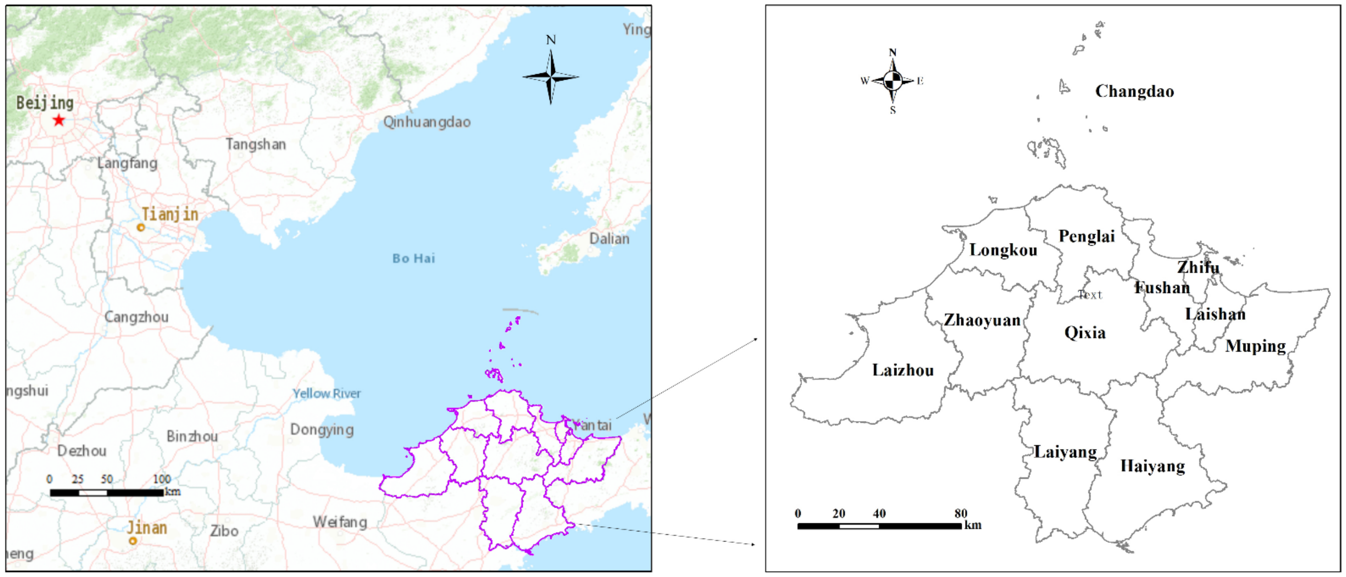
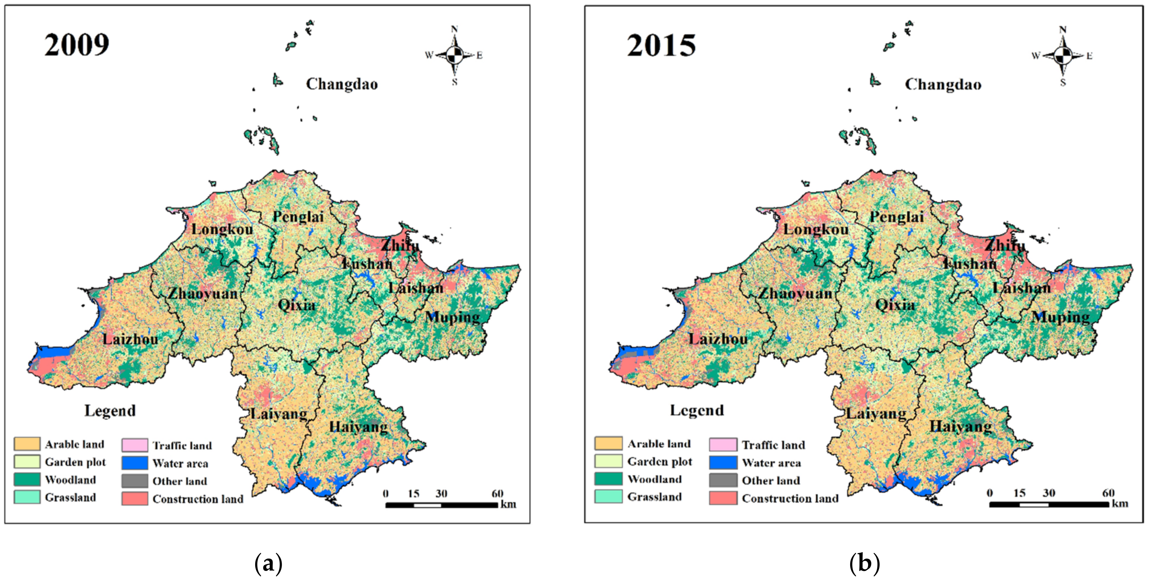
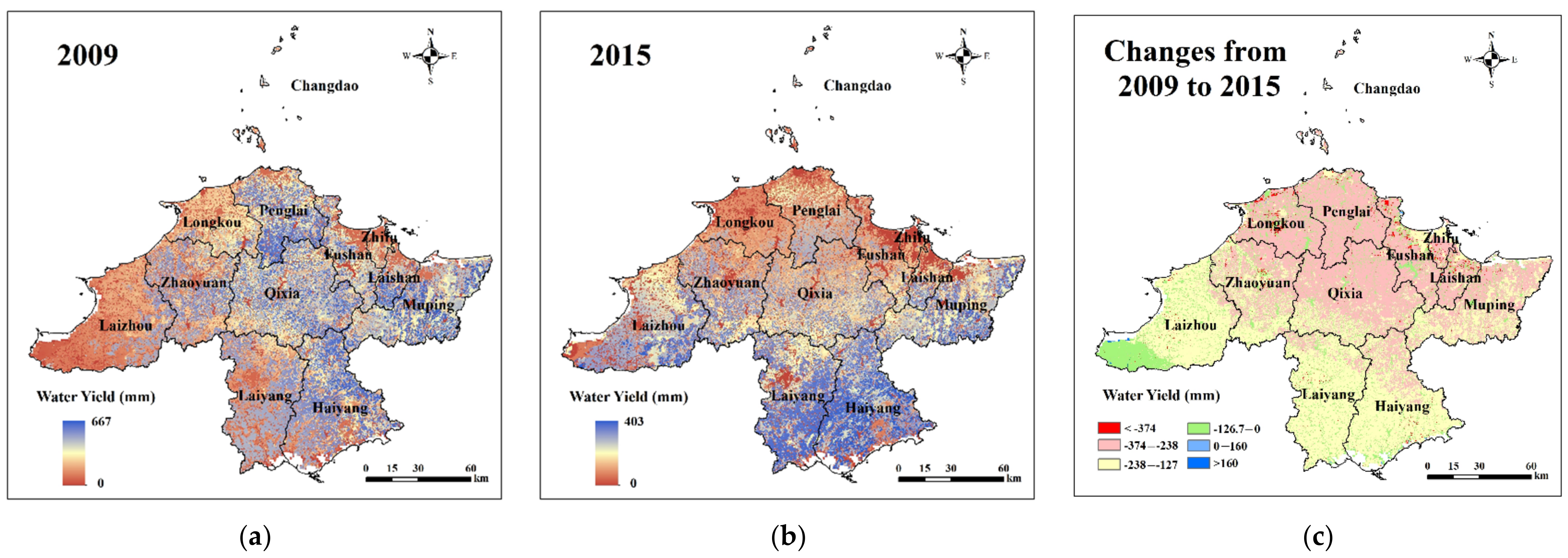
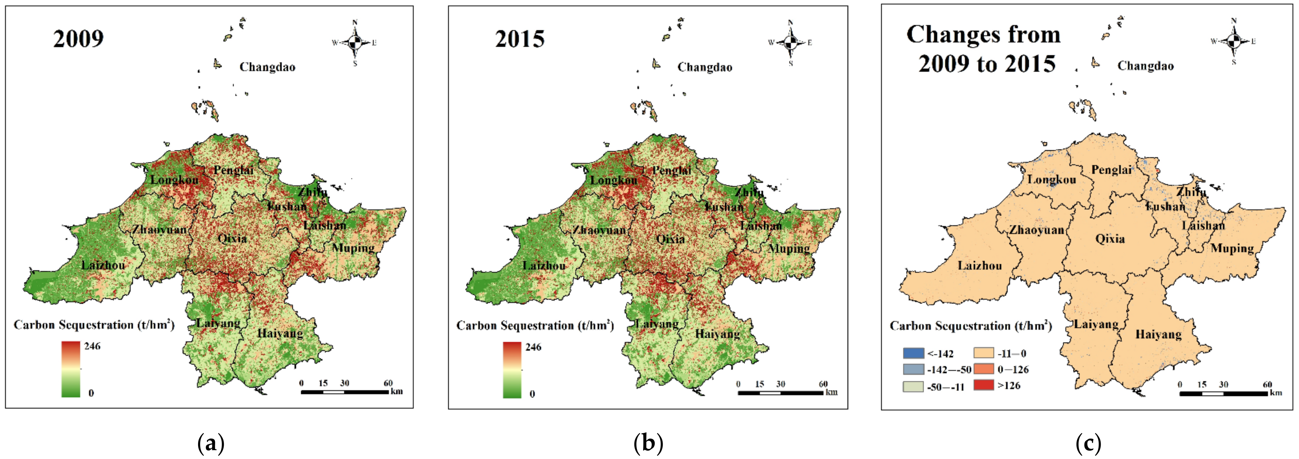
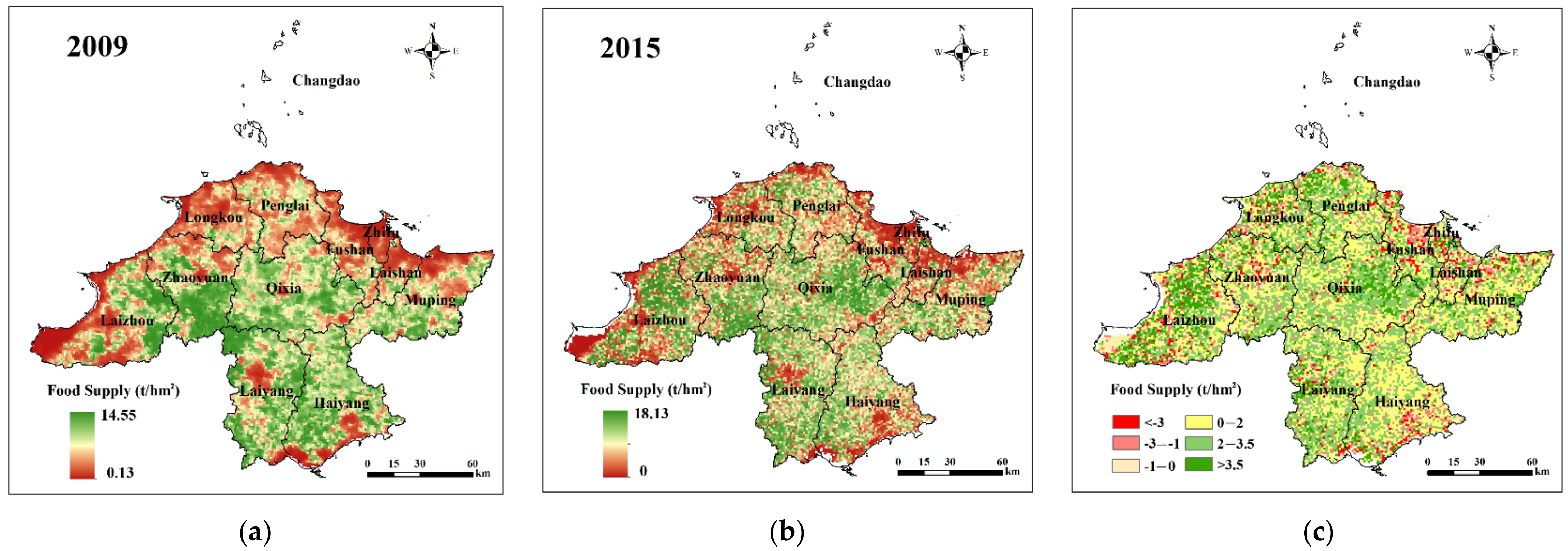
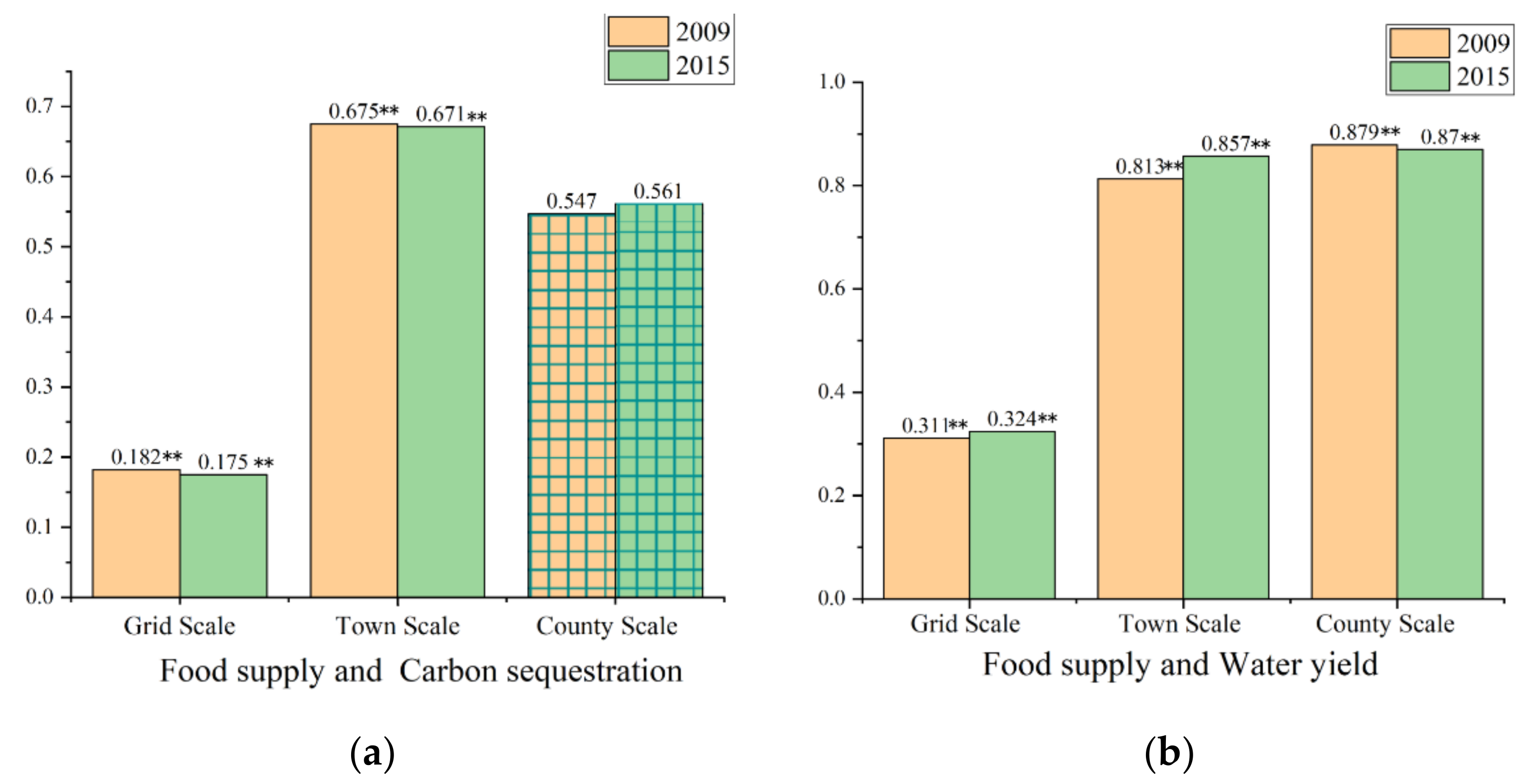
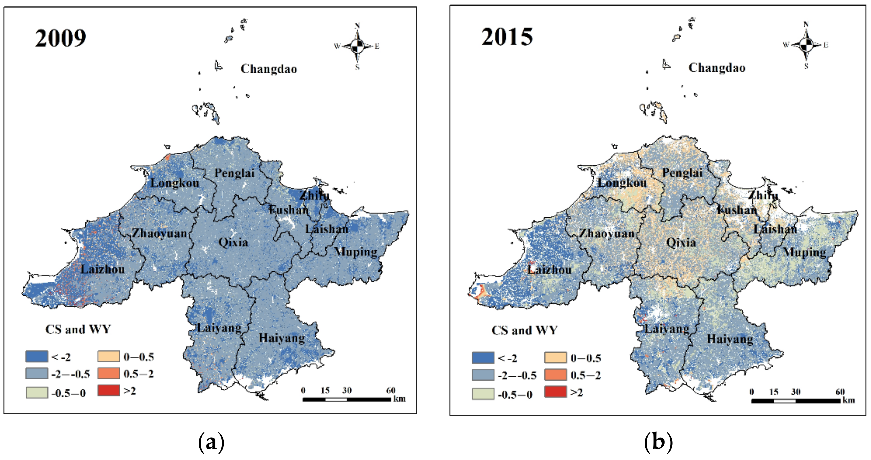
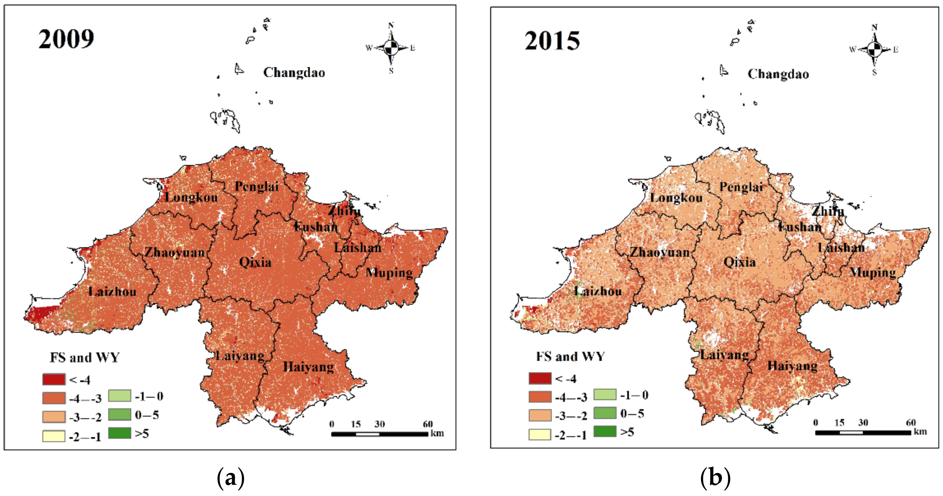
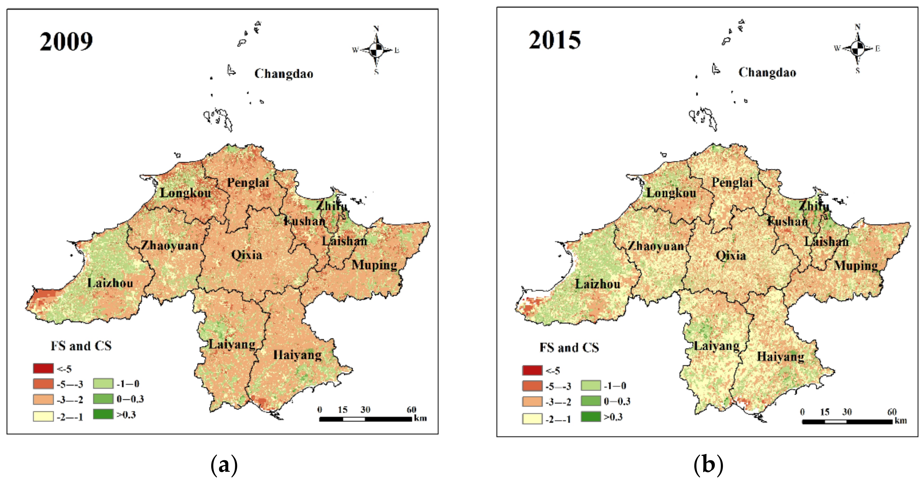
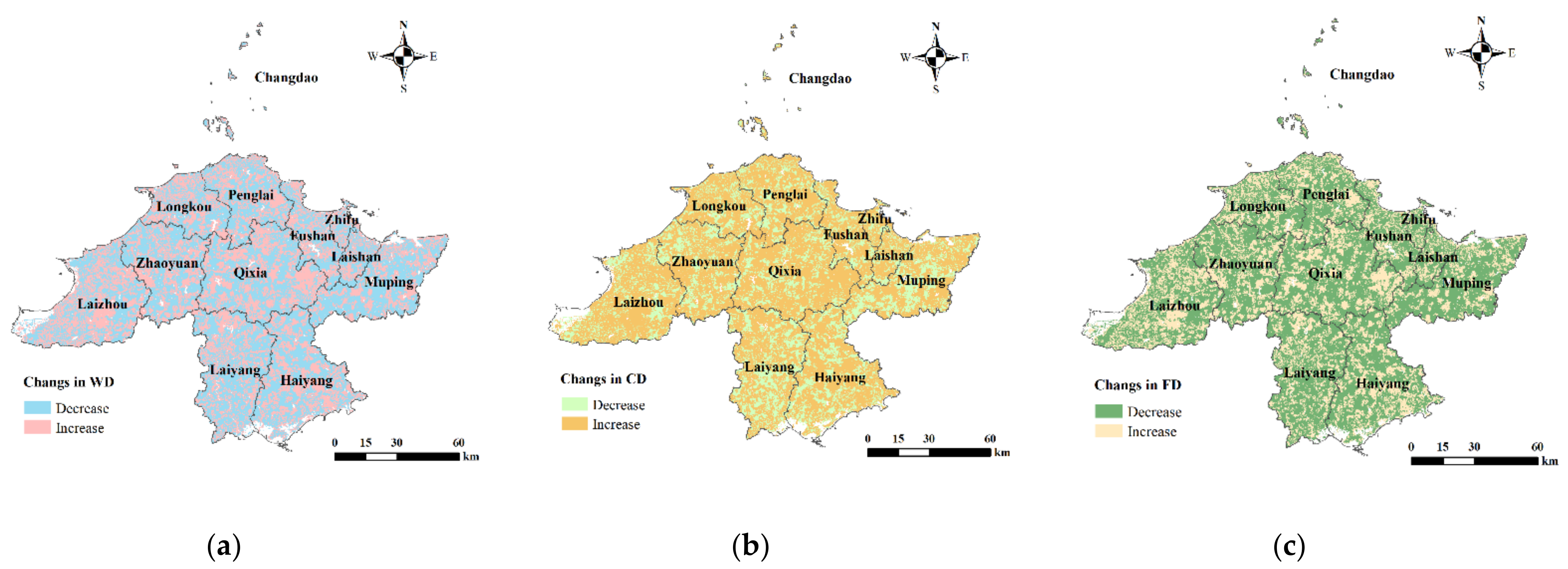
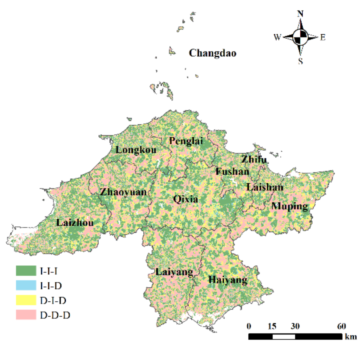
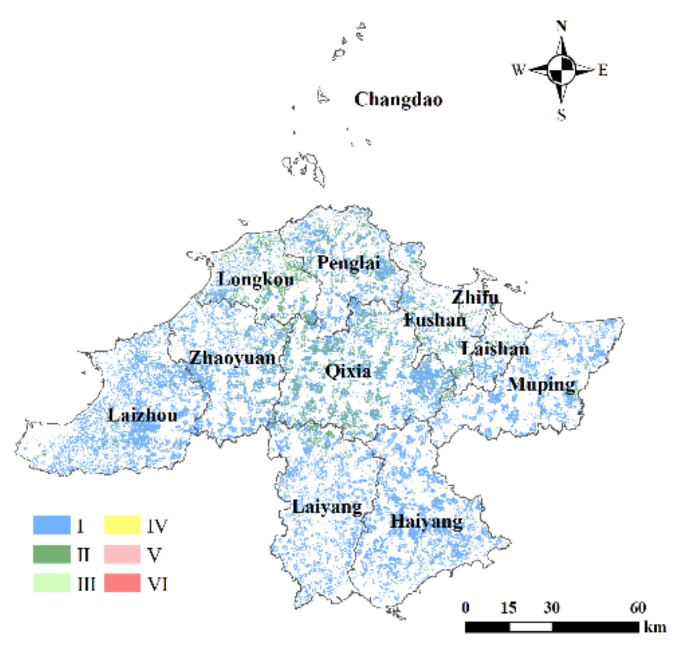
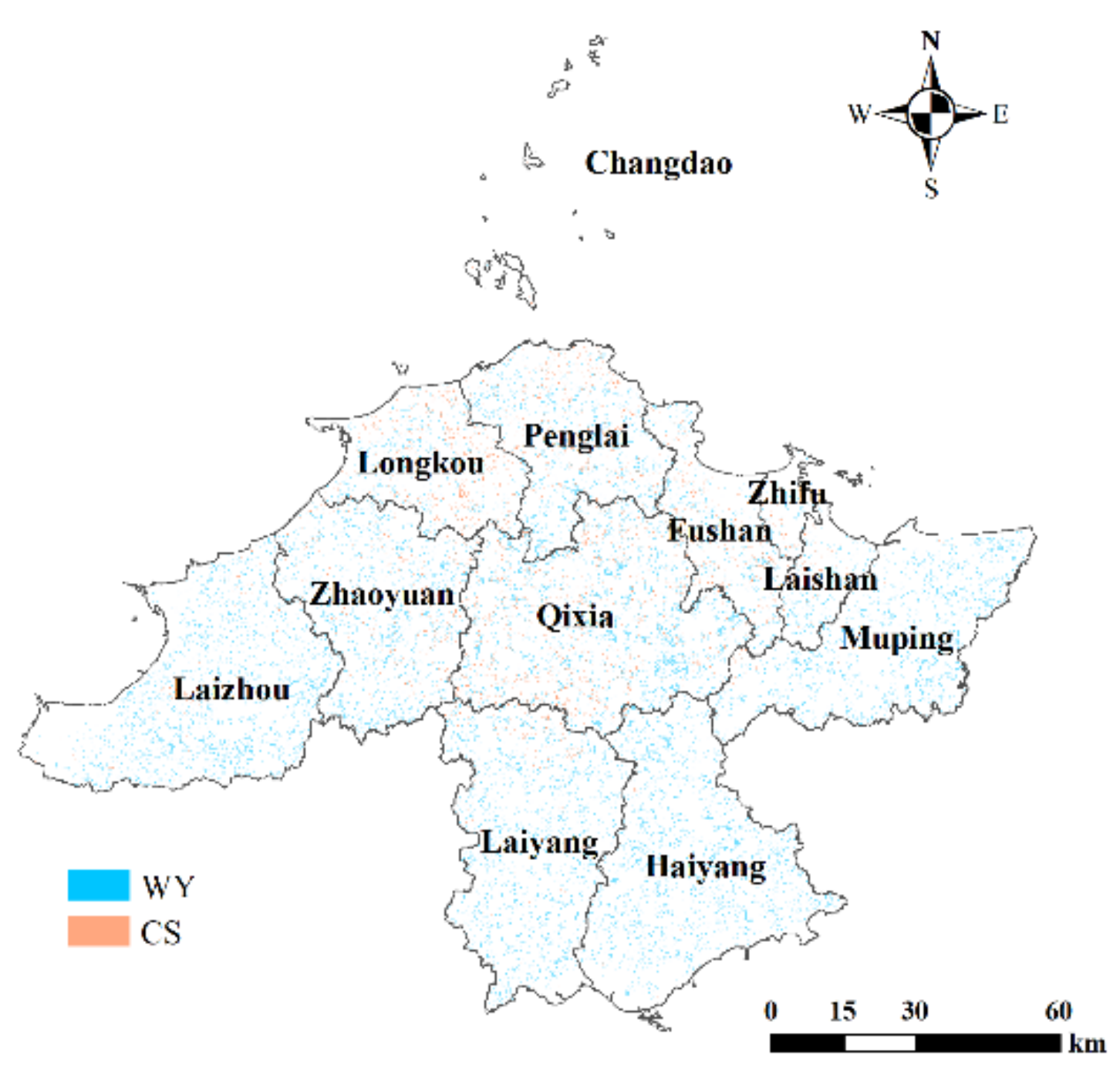
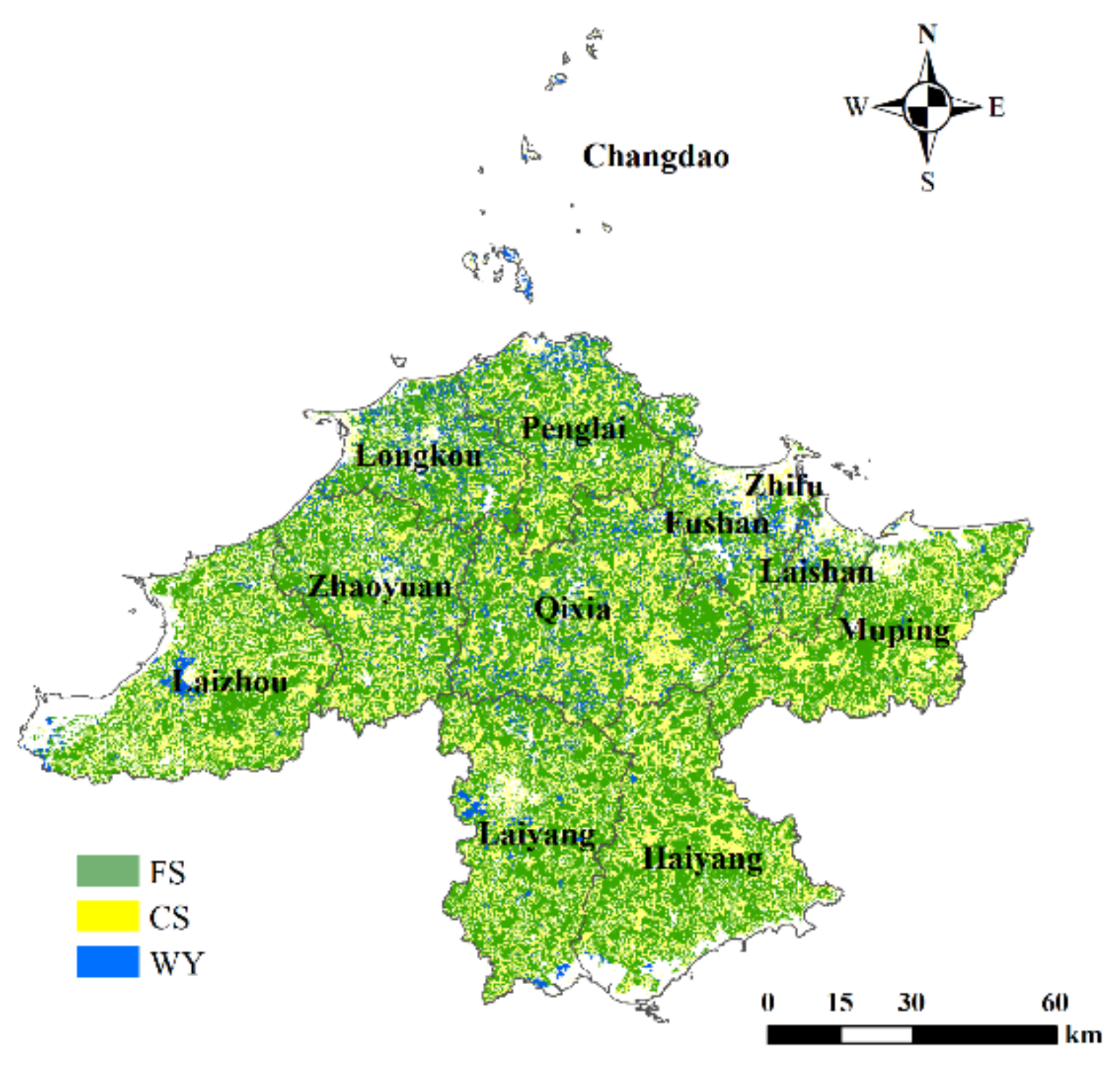
Table 1.
Biophysical table used for the baseline InVEST water yield model run.
| Land Use Class | Kc | Root_Depth (mm) | Land Use_Veg |
|---|---|---|---|
| Paddy land | 0.7 | 700 | 1 |
| Irrigated land | 0.7 | 500 | 1 |
| Dry land | 0.2 | 100 | 1 |
| Orchard | 0.7 | 3000 | 1 |
| Tea plantation | 0.5 | 2000 | 1 |
| Other garden | 0.5 | 1500 | 1 |
| Forest land | 1 | 7000 | 1 |
| Shrub land | 0.5 | 5000 | 1 |
| Other woodland | 0.7 | 2500 | 1 |
| Artificial herbage land | 0.65 | 2500 | 1 |
| Other grassland | 0.65 | 2500 | 1 |
| Railway | 0.1 | 50 | 0 |
| Highway | 0.2 | 100 | 0 |
| Rural road | 0.1 | 50 | 0 |
| Airport land | 0.1 | 100 | 0 |
| Port and wharf land | 0.1 | 50 | 0 |
| River | 1 | 1000 | 0 |
| Lake | 0.9 | 1000 | 0 |
| Reservoir | 1 | 1000 | 0 |
| Pit and pond | 1 | 1000 | 0 |
| Tidal flat | 0.7 | 1000 | 0 |
| Interior tideland | 0.7 | 1000 | 0 |
| Ditch | 1 | 500 | 0 |
| Hydraulic construction land | 0.1 | 300 | 0 |
| Agricultural facility land | 0.15 | 300 | 0 |
| Saline-alkali land | 0.5 | 10 | 0 |
| Sand | 0.5 | 10 | 0 |
| Bare land | 0.2 | 10 | 0 |
| Urban | 0.3 | 500 | 0 |
| Town | 0.3 | 500 | 0 |
| Village | 0.4 | 500 | 0 |
| Mining land | 0.3 | 500 | 0 |
| Scenic spots and special land | 0.3 | 500 | 0 |
Table 2.
Biomass and soil carbon density (Mg/ha) in different land use class.
| Land Use Class | Cabove | Cbelow | Csoil | Cdead |
|---|---|---|---|---|
| Paddy land | 5 | 3 | 15 | 0 |
| Irrigated land | 5 | 5 | 15 | 0 |
| Dry land | 5.6 | 1.12 | 93 | 2 |
| Orchard | 125 | 5 | 115 | 1 |
| Tea plantation | 10 | 3 | 90 | 1 |
| Other garden | 8 | 5 | 20 | 0 |
| Forest land | 19.4 | 3.88 | 127.3 | 1.94 |
| Shrub land | 8 | 8 | 25 | 3 |
| Other woodland | 10 | 3 | 90 | 1 |
| Artificial herbage land | 0.439 | 5.05 | 100 | 0.21 |
| Other grassland | 0.233 | 1.559 | 100 | 0.21 |
| Railway | 0 | 0 | 25 | 0 |
| Highway | 0 | 0 | 40 | 0 |
| Rural road | 0 | 0 | 35 | 0 |
| Airport land | 0 | 0 | 30 | 0 |
| Port and wharf land | 0 | 0 | 20 | 0 |
| River | 0.6 | 0.12 | 81.7 | 0.06 |
| Lake | 0.6 | 0.12 | 81.7 | 0.06 |
| Reservoir | 0.6 | 0.12 | 81.7 | 0.06 |
| Pit and pond | 0.6 | 0.12 | 81.7 | 0.06 |
| Tidal flat | 10 | 5 | 20 | 0 |
| Interior tideland | 10 | 5 | 20 | 0 |
| Ditch | 0 | 0 | 0 | 0 |
| Hydraulic construction land | 0.1 | 0.2 | 10 | 0.01 |
| Agricultural facility land | 0.1 | 0.2 | 30 | 0.01 |
| Saline-alkali land | 0 | 0 | 0 | 0 |
| Sand | 0.1 | 0.2 | 11.7 | 0.01 |
| Bare land | 0.1 | 0.2 | 11.7 | 0.01 |
| Urban | 0.1 | 0.2 | 10 | 0.01 |
| Town | 0.1 | 0.2 | 30 | 0.01 |
| Village | 0 | 0 | 50 | 1 |
| Mining land | 0 | 0 | 10 | 0 |
| Scenic spots and special land | 0 | 0 | 10 | 0 |
Table 3.
Classification rule of changes in ecosystem services demands from 2009 to 2015.
| Ecosystem Services Demand | WD | CD | FD | |
|---|---|---|---|---|
| Type | ||||
| I-I-I | Increase | Increase | Increase | |
| I-I-D | Increase | Increase | Decrease | |
| I-D-I | Increase | Decrease | Increase | |
| I-D-D | Increase | Decrease | Decrease | |
| D-I-I | Decrease | Increase | Increase | |
| D-I-D | Decrease | Increase | Decrease | |
| D-D-I | Decrease | Decrease | Increase | |
| D-D-D | Decrease | Decrease | Decrease | |
| I-I-I | Increase | Increase | Increase | |
Table 4.
Classification rule of dominant ecosystem service in the synergies in 2015.
| Type | Synergies | Dominant Ecosystem Service | Synergies | Dominant Ecosystem Service | Synergies | Dominant Ecosystem Service |
|---|---|---|---|---|---|---|
| I | WY-CS | WY | WY-FS | WY | CS -FS | CS |
| II | WY-CS | CS | WY-FS | WY | CS -FS | CS |
| III | WY-CS | CS | WY-FS | FS | CS -FS | CS |
| IV | WY-CS | WY | WY-FS | WY | CS -FS | FS |
| V | WY-CS | WY | WY-FS | FS | CS -FS | FS |
| VI | WY-CS | CS | WY-FS | FS | CS -FS | FS |
| VII | WY-CS | WY | WY-FS | FS | CS -FS | CS |
| VIII | WY-CS | CS | WY-FS | WY | CS -FS | FS |
Table 5.
The land-use transfer matrix 1 of Yantai from 2009 to 2015 (km2).
| 2015 | 2009 | |||||||
|---|---|---|---|---|---|---|---|---|
| Arable Land | Garden Plot | Woodland | Grassland | Traffic Land | Water Area | Other Land | Construction Land | |
| Arable land | 5436.2 | 4.36 | 5.43 | 17.28 | 0.08 | 0.92 | 1.92 | 5.34 |
| Garden plot | 0.55 | 2417.3 | 0.09 | 0.17 | 0.15 | 0 | 0 | 1.58 |
| Woodland | 2.29 | 0.68 | 2235.97 | 0.32 | 0 | 0.74 | 0.12 | 0.27 |
| Grassland | 0 | 0 | 0.55 | 626.94 | 0.05 | 0.34 | 0.05 | 0.09 |
| Traffic land | 18.2 | 11.24 | 3.51 | 2.16 | 134.19 | 1.86 | 1.54 | 0.98 |
| Water area | 0.51 | 0.2 | 0.39 | 0.12 | 0.01 | 824.3 | 0.04 | 0.01 |
| Other land | 13.31 | 5.28 | 4.2 | 2.13 | 0 | 18.9 | 298.46 | 0.18 |
| Construction land | 51.32 | 45.99 | 12.73 | 15.03 | 0.06 | 12 | 6.98 | 1607.08 |
1 Column means land use type in 2009 and row means land use type in 2015. For a type of land use, the cell with same name in column and row means the unchanged area from 2009 to 2015. Except this value, other values in the row mean increased area changed from other land use types while other values in the column mean the area changed into other land use types from 2009 to 2015.
Table 6.
Improvement priority in I-I-I in 2015.
| Type | Proportion | Prior Improvement Ecosystem Service |
|---|---|---|
| I | 83.58% | FS |
| II | 14.88% | FS |
| III | 0.21% | WY |
| IV | 1.16% | CS |
| V | 0.03% | CS |
| VI | 0.13% | WY |
Table 7.
Improvement priority in D-D-D in 2015.
| Type | Proportion | Prior Improvement Ecosystem Service | Service Region | Services Provided |
|---|---|---|---|---|
| I | 85.42% | FS | I-I-I (III, VI), I-I-D(CS-dominated) | WY |
| II | 13.01% | FS | I-I-I (IV, V), I-I-D(WY-dominated), D-I-D | CS |
| III | 0.23% | WY | I-I-I (IV, V), I-I-D(WY-dominated), D-I-D | CS |
| IV | 1.20% | CS | I-I-I (III, VI), I-I-D(CS-dominated) | WY |
| V | 0.03% | CS | I-I-I (I, II) | FS |
| VI | 0.11% | WY | I-I-I(I, II) | FS |
Publisher’s Note: MDPI stays neutral with regard to jurisdictional claims in published maps and institutional affiliations. |
© 2021 by the authors. Licensee MDPI, Basel, Switzerland. This article is an open access article distributed under the terms and conditions of the Creative Commons Attribution (CC BY) license (https://creativecommons.org/licenses/by/4.0/).
Share and Cite
MDPI and ACS Style
Fang, Y.; Zhai, T.; Zhao, X.; Chen, K.; Guo, B.; Wang, J. Study on the Comprehensive Improvement of Ecosystem Services in a China’s Bay City for Spatial Optimization. Water 2021, 13, 2072. https://doi.org/10.3390/w13152072
AMA Style
Fang Y, Zhai T, Zhao X, Chen K, Guo B, Wang J. Study on the Comprehensive Improvement of Ecosystem Services in a China’s Bay City for Spatial Optimization. Water. 2021; 13(15):2072. https://doi.org/10.3390/w13152072
Chicago/Turabian StyleFang, Ying, Tianlin Zhai, Xiaodong Zhao, Kun Chen, Baishu Guo, and Jing Wang. 2021. "Study on the Comprehensive Improvement of Ecosystem Services in a China’s Bay City for Spatial Optimization" Water 13, no. 15: 2072. https://doi.org/10.3390/w13152072
Note that from the first issue of 2016, this journal uses article numbers instead of page numbers. See further details here.