Monitoring Crop Evapotranspiration and Transpiration/Evaporation Partitioning in a Drip-Irrigated Young Almond Orchard Applying a Two-Source Surface Energy Balance Model

Abstract

Encouraged by the necessity to better understand the water use in this woody crop, a study was carried out in a commercial drip-irrigated young almond orchard to quantify and monitor the crop evapotranspiration (ET_c) and its partitioning into tree canopy transpiration (T) and soil evaporation (E), to list and analyze single and dual crop coefficients, and to extract relationships between them and the vegetation fractional cover (f_c) and remote-sensing-derived vegetation indices (VI_s). A Simplified Two-Source Energy Balance (STSEB) model was applied, and the results were compared to ground measurements from a flux tower. This study comprises three consecutive growing seasons from 2017 to 2019, corresponding to Years 2 to 4 after planting. Uncertainties lower than 50 W m⁻² were obtained for all terms of the energy balance equation on an instantaneous scale, with average estimation errors of 0.06 mm h⁻¹ and 0.6 mm d⁻¹, for hourly and daily ET_c, respectively. Water use for our young almond orchard resulted in average mid-season crop coefficient (K_{c mid}) values of 0.30, 0.33, and 0.45 for the 2017, 2018, and 2019 growing seasons, corresponding to f_c mean values of 0.21, 0.35, and 0.39, respectively. Average daily evapotranspiration for the same periods resulted in 1.7, 2.1, and 3.2 mm d⁻¹. The results entail the possibility of predicting the water use of any age almond orchards by monitoring its biophysical parameters.

1. Introduction

The global planted area and production of almonds are steadily increasing. According to the Food and Agriculture Organization Corporate Statistical Database (FAOSTAT) [1], more than 2 million ha of almond orchards are cultivated worldwide. Spain ranks first in planted area with almonds in the world, with more than 650,000 ha, followed by the western United States of America (USA) with about 441,000 ha. However, the USA leads the production, accounting for 77% of the world crop share in 2019, whereas Spain only contributes a 6% of the share [2]. This is due to the low average yields obtained in our country as almond trees are mainly grown under rainfed conditions and on marginal soils in areas where annual rainfall ranges from 250 to 350 mm [3]. Nevertheless, the surface area of irrigated almond orchards has increased considerably in Spain in recent years, currently representing about 14% of the harvested almond area. This work focuses on the La Mancha region, where evaporative demand is high and rainfall is scarce during the summer, coinciding with the highest crop water requirements. In this region, almonds covered about 124,000 ha in 2018, and irrigation is expanding every year in order to increase the profitability of orchards, already representing 16% (almost 20,000 ha) of the harvested almond area [3,4].

In arid and semi-arid areas with water resources scarcity, population growth and increasing water competition with other sectors, such as industrial and urban, improvement of almond water management becomes mandatory. In addition, in a global scenario of climate change, this situation seems to be worsening, mainly due to higher temperatures, less annual rainfall and an increasing number of extreme weather events [5]. Under this context, in the study area, where water resources (mainly groundwater) are limited and at serious risk of overexploitation, it is not possible to apply irrigation regimes that cover the potential crop water requirements of almond trees. Therefore, measuring or estimating almond crop evapotranspiration (ET_c), and deriving its crop coefficients as accurately as possible, becomes a key objective for optimizing the irrigation scheduling of this fruit tree.

ET_c is usually calculated or modelled adopting the FAO56 approach [6,7,8]. This method uses the grass reference evapotranspiration (ET_o) multiplied by a crop coefficient (K_c). Moreover, the FAO56 method also offers the possibility of ET_c partitioning, i.e., distinguishing soil evaporation (E) from crop transpiration (T) by using a dual crop coefficient approach (ET_c = (K_cb + K_e) × ET_o), where K_cb is a basal (transpiration) crop coefficient and K_e is a soil evaporation coefficient. This simple approach is considered the standard by the scientific community for vegetables and field crops (i.e., full and homogeneous canopies), but it is especially challenging for fruit trees and vines due to the wide range of plant densities, canopy architectures, crop age and varieties, fraction of ground cover, management and training classes, etc. Therefore, other methods may be used for estimating ET_c, mainly based on remote sensing techniques [9,10].

Over the last two decades, a huge number of articles have been published reporting standardized K_c values for almost all cultivated crops and environmental conditions. However, studies on accurate ET_c measurements and deriving K_c values for young almond orchards are quite scarce [11,12]. Besides, there are new varieties of late and extra-late flowering, which have not been sufficiently studied and require an adjustment of their K_c in order to conduct a more precise irrigation scheduling [13].

In FAO66, Goldhamer and Girona [14] reported monthly K_c values for mature almond trees published by different authors [15,16,17]. Those studies mainly measured almond ET_c using a soil water balance approach rather than more precise methods such as weighing lysimeters or eddy-covariance (EC) systems. Seasonal ET_c and K_c values were determined for a high-yielding almond orchard using an EC flux heat system in South Australia [18]. Espadafor et al. [11] measured transpiration of young almond trees using a large weighing lysimeter in Córdoba (Spain). In the same research facility, López-López et al. [19] reported water requirements of mature almond trees combining measurements of a weighing lysimeter with sap-flow probes. In an experiment performed only along one growing season in southwest Spain, García-Tejero et al. [12] reported local crop coefficients for young almond trees using four drainage lysimeters. In a study conducted in Central Valley (California), Bellvert et al. [9] estimated actual crop evapotranspiration and K_c values of an almond orchard during a single crop season. These authors combined a simple ET_c model with remote sensing techniques.

Surface energy balance models have been long used to derive ET_c values in a wide variety of environmental and ecosystem conditions [20,21,22,23,24,25,26,27,28,29,30]. Land surface temperature (LST) is a key input in these model schemes, and the thermal characterization of row crops becomes a challenge in comparison to more homogeneous canopies such as vegetables (e.g., roots and tubers) or field crops (e.g., cereals). Soil evaporation might not be negligible in this type of crop, and this component must be accounted for in ET_c estimates. Two-source energy balance techniques, together with ground measurements of soil and canopy temperatures, have provided good results in different field crops, such as cotton [20,27], maize [29,31,32] or vineyard [30]. Orchard-row crops bring additional limitations related to the canopy structure itself and the low canopy cover that increase the significance of the inter-row vegetation maintenance in the surface flux patterns. This effect is stressed in young orchards.

In this work, a Simplified version of the Two-Source Energy Balance (STSEB) was used, together with field measurements of soil and canopy temperatures, to model the surface energy flux balance in a young almond orchard and to partition the ET_c into canopy and soil components. A separate monitoring of the soil evaporation (E) and canopy transpiration (T), together with the total ET_c, was established. This allowed for a comprehensive analysis of the dual crop coefficients, which is not possible using only weighing lysimeters or eddy-covariance measurements.

The main objectives of this work were to:

• Evaluate the performance of the STSEB approach, combined to radiometric temperature measurements, in almond orchard using an eddy-covariance system. Ground measurements of the surface energy fluxes were used as a basis for the assessment.
• Derive single and dual crop coefficients of the drip-irrigated young almond orchard using STSEB and ET_o estimates.
• Explore relationships between crop coefficients and biophysical variables and vegetation indices that can be further applied to almond orchards under a range of growing stage and environmental conditions.

2. Materials and Methods

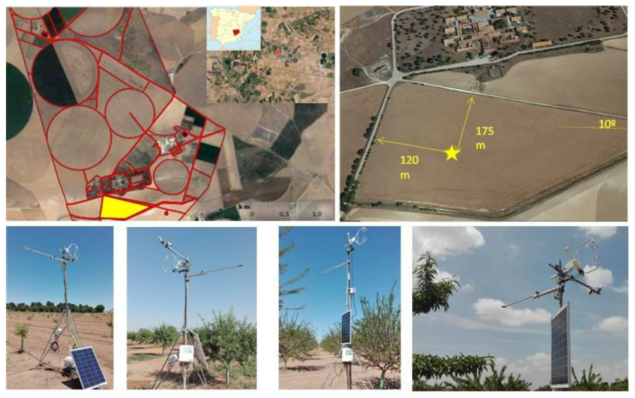
2.1. Study Site

The study is based on measurements conducted during three consecutive almond growing seasons from 2017 to 2019 at the Technical Institute of Agronomy (ITAP) Research Facility in Albacete (southeast Spain) (39°2′ N, 2°5′ W, 695 m a.s.l) (Figure 1). The climate is semi-arid, temperate Mediterranean with dry and warm summers resulting in a high evaporative demand. The long-term (30-year) mean annual precipitation is 314 mm mostly concentrated during the months of spring and autumn, and average mean, maximum and minimum air temperatures are 13.8, 24.6 and 4.8 °C, respectively. Weather data were recorded for a 30-year period (1987–2016) from an automated agro-meteorological station located at the study site. According to the Soil Survey Staff [33], the soil at this site is classified as Petrocalcic Calcixerepts, with a loam texture (31.6% sand, 42.4% silt and 26% clay), with a basic pH (8.4). The soil has a content of organic matter, nitrogen and active limestone of 1.55%, 0.09%, and 12.1%, respectively. Soil electrical conductivity (ECe) was 0.35 dS m⁻¹, resulting in a slightly saline soil.

2.2. Orchard Description

Measurements were carried out in a young almond (Prunus dulcis (Mill.) D.A. Webb) orchard of about 11 ha planted in 2015 with ‘Lauranne’ grafted onto the GF-677 rootstock. Tree spacing was 6 m (within row) and 7 m (inter-row), giving 238 trees ha⁻¹. Drip-irrigation was supplied during the experiment with a single drip line per row with 3.2 L h⁻¹ emitters spaced every 0.75 m. The field was fertilized at a rate from 95-40-85 kg ha⁻¹ of N, P and K to 160-84-140 kg ha⁻¹ of N, P and K in the first and the last experimental season, respectively; it was managed according to cultural practices usually carried out in the area, to avoid pests and disease effects on crop performance.

Irrigation in the almond orchard was managed following the common practice in the area for accomplishing potential (maximum) yields. Irrigation was scheduled based on the soil water balance approach, by estimating ET_c (crop water requirements) through the FAO56 approach, i.e., as the product of Penman–Monteith ET_o [6] by a crop coefficient (K_c) [16]. Since the fraction of green ground cover (f_c) remained below 70% in our study, an empirical reduction coefficient (K_r) was used for computing ET_c, i.e., ET_c = ET_o × K_c × K_r [34].

Almond tree structure was monitored during the experiment. Frequent in situ measurements of horizontal diameters of the canopy and tree height were taken during the three cropping seasons. Moreover, ground nadir digital pictures of five representative trees were sampled overhead during the last season. All these ground measurements were combined and used to model f_c for the three growing seasons (Figure 2).

2.3. Eddy-Covariance and Meteorological Instrumentation

An eddy-covariance system was used in this work for the assessment of the ET_c derived values from the STSEB model. The flux tower was assembled in a central location of the field at the beginning of the 2016 growing season, although instrumentation was not completed until 2017 (Figure 1). The flux tower was provided with a net radiation sensor (NR-Lite, Kipp & Zonen, Delft, The Netherlands), and a set of 2–4 heat flux plates (HFP01SC, Hukseflux, Delft, the Netherlands) buried at 8 cm depth, at both side of the row. Soil temperature was measured by thermocouples (TCAV, Type E, Campbell Sci. Inst., Logan, UT, USA) at 2 and 4 cm depth, and soil moisture was measured by volumetric moisture sensors (CS650, Campbell Sci. Inst., Logan, UT, USA) to account for the heat storage in the soil layer above the plates. All these data were stored in 15 min averages using a datalogger (CR1000, Campbell Sci. Inst., Logan, UT, USA) and then processed to derive hourly fluxes.

The turbulent fluxes were measured by an eddy-covariance (EC) system mounted on the tripod (Figure 1) and were oriented to the dominant winds coming from the west. It consisted of a sonic anemometer (CSAT-3, Campbell Sci. Inst., Logan, UT, USA) and an open-path infrared gas analyzer (LI-7500, LI-COR Inc., Lincoln, NE, USA). The EC instruments were originally emplaced at a height of 4 m in this experiment to avoid contribution of surrounding areas beyond the almond field boundaries. A footprint analysis was conducted to support this configuration. This position was raised up to 5 m for the 2019 season to keep a minimum distance of 1.5 m with the canopy top.

The study period ranged from 16 June to 16 October (4 months) in 2017, 3 May to 18 October (5.5 months) in 2018, and 15 April to 21 September (5 months) in 2019. The dataset covered the full Stage III phenological phase (increase in weight of seed) for the 3 years, and a good portion of Stage II (growth of embryo) and Stage IV (post-harvest). A total of >400 days were considered within these periods once a few days had been discarded due to bad weather conditions and experimental failures.

Meteorological data during the 3-year experiment were measured with a weather station located in the Research Facility near the almond orchard. All instruments were set up at a height between 1.5 and 2.0 m above the ground surface, and weather data were registered in 15 min, hourly and daily time steps. The variables measured were as follows: incoming and surface-reflected short-wave radiation (model CM14, Kipp & Zonen, Delft, Holland), incoming and outgoing long-wave radiation (model CG2, Kipp & Zonen, Delft, Holland), air temperature/relative humidity (model MP100, Campbell Scientific Instrument, Logan, UT, USA), wind speed (model A100R, Vector Instruments Ltd., Rhyl, UK), wind direction (model W200P, Vector Instruments Ltd., Rhyl, UK) and rainfall (model ARG100, Campbell Scientific Instrument, Logan, UT, USA). All meteorological data were recorded with two CR10X data loggers (Campbell Scientific Instrument, Logan, UT, USA). Daily ET_o was computed with the FAO56 Penman–Monteith equation [6]. López-Urrea et al. [35] and Trigo et al. [36] carried out previous studies in the experimental site reporting the good performance of this method. The single crop coefficient (K_c) for young almond trees was obtained as the ratio of the ET_c determinations to the calculated ET_o values, whereas the dual K_c was calculated as the ratios of T and E estimations using the STSEB approach to ET_o, i.e., K_cb = T/ET_o and K_e = E/ET_o.

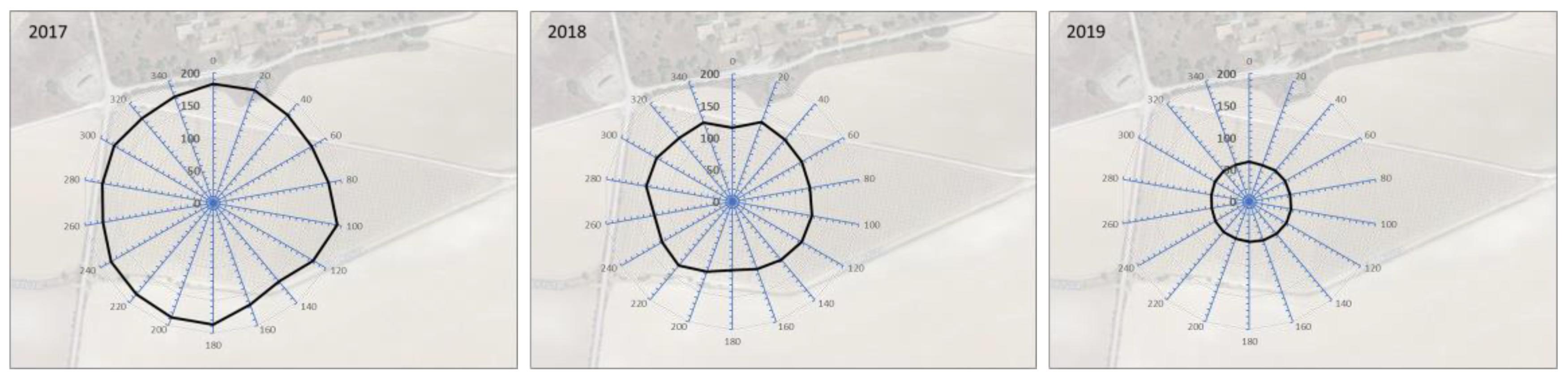
2.4. Footprint Analysis and Adjustment of Turbulent Fluxes

The relatively small size of the studied almond orchard field is a challenge since the footprint area contributing to the turbulent flux measurements must remain within the parcel limits, while a certain position over the canopy top is recommended to capture all eddies. Based on a successful previous experience in a close vineyard using the same EC system, we decided to set the EC instruments initially at a height of 4 m above ground level for the 2017–2018 experimental campaigns and raised up to 5 m for the 2019 season. The footprint analysis [37] showed that 90% of cumulative normalized flux measurements were obtained within average upwind distances of 178 ± 23 m, 125 ± 42 m and 63 ± 5 m in 2017, 2018 and 2019, respectively. Figure 3 plots the average footprint for the different wind directions. Note that the footprint fits within the field boundary in 2018 and 2019, whereas 25% of the dataset outlies this limit in 2017 due to the short canopy height of the almond trees. This fraction of the dataset can be discarded, although no significant changes in the analysis were observed, which indicates that the influence of the surrounding areas was minor in our case.

To guarantee the highest quality in the turbulent flux measurements, energy balance closure was also checked and forced by using the residual technique [38].

2.5. The STSEB Approach Combined with Ground Radiometric Thermal Measurements

Two-Source Energy Balance modeling of crop evapotranspiration (ET_c), and its soil evaporation (E) and canopy transpiration (T) contributions, is conceived as a conversion from the total latent heat flux, LE, and its soil and canopy components LE_s and LE_c, respectively, dividing by the latent heat of vaporization of water, λ (J kg⁻¹). The latent heat flux is a turbulent flux that can be estimated as a residual from the surface energy balance equation (Equation (1)) once known the other terms:

$${\mathrm{R}}_{\mathrm{n}}=\mathrm{H}+\mathrm{LE}+\mathrm{G}$$

(1)

where R_n is the net radiation flux (W m⁻²), H is the sensible heat flux (W m⁻²), and G is the soil heat flux (W m⁻²).

Based on the parallel approach introduced by [21], a Simplified version of the Two-Source Energy Balance (STSEB) model was initially proposed by [29]. This model allows one to estimate the surface energy fluxes using radiometric temperatures of the canopy (T_c) and soil (T_s) components as the key input in the different terms of the energy balance equation. Following the STSEB approach, the addition between the soil (H_s) and canopy (H_c) contributions, to the total sensible heat flux, are weighted by their respective cover fraction as follows:

$$\mathrm{H}={\mathrm{f}}_{\mathrm{c}}{\mathrm{H}}_{\mathrm{c}}+(1-{\mathrm{f}}_{\mathrm{c}}){\mathrm{H}}_{\mathrm{s}}$$

(2)

In Equation (2), H_s and H_c are expressed as:

$${\mathrm{H}}_{\mathrm{c}}={\mathsf{\rho }\mathrm{C}}_{\mathrm{p}}\frac{{\mathrm{T}}_{\mathrm{c}}-{\mathrm{T}}_{\mathrm{a}}}{{\mathrm{r}}_{\mathrm{a}}^{\mathrm{h}}}$$

(3)

$${\mathrm{H}}_{\mathrm{s}}={\mathsf{\rho }\mathrm{C}}_{\mathrm{p}}\frac{{\mathrm{T}}_{\mathrm{s}}-{\mathrm{T}}_{\mathrm{a}}}{{\mathrm{r}}_{\mathrm{a}}^{\mathrm{a}}+{\mathrm{r}}_{\mathrm{a}}^{\mathrm{s}}}$$

(4)

where ρC_p is the volumetric heat capacity of air (J K⁻¹m⁻³), T_a is the air temperature at a reference height (K), ${\mathrm{r}}_{\mathrm{a}}^{\mathrm{h}}$ is the aerodynamic resistance (s m⁻¹) to heat transfer between the canopy and the reference height at which the atmospheric data are measured (m), ${\mathrm{r}}_{\mathrm{a}}^{\mathrm{a}}$ is the aerodynamic resistance (s m⁻¹) to heat transfer between the point $z_{0M}$+d ($z_{0M}$: canopy roughness length for momentum, d: displacement height) and the reference height (m), ${\mathrm{r}}_{\mathrm{a}}^{\mathrm{s}}$ is the aerodynamic resistance (s m⁻¹) to heat flow in the boundary layer immediately above the soil surface. For details on the expressions to estimate these aerodynamic resistances, see [29].

The STSEB approach conceives the partitioning of the net radiation flux, R_n, between the soil and canopy as follows:

$${\mathrm{R}}_{\mathrm{n}}={\mathrm{f}}_{\mathrm{c}}{\mathrm{R}}_{\mathrm{nc}}+(1-{\mathrm{f}}_{\mathrm{c}}){\mathrm{R}}_{\mathrm{ns}}$$

(5)

where R_nc and R_ns are the contributions of the canopy and soil, respectively, to the total net radiation flux. A balance is established between the longwave and the short-wave radiation separately for each component:

$${\mathrm{R}}_{\mathrm{nc}}=\left(1-{\mathsf{\alpha }}_{\mathrm{c}}\right)\mathrm{S}+{\mathsf{\epsilon }}_{\mathrm{c}}{\mathrm{L}}_{\mathrm{sky}}-{\mathsf{\epsilon }}_{\mathrm{c}}{\mathsf{\sigma }\mathrm{T}}_{\mathrm{c}}^4$$

(6)

$${\mathrm{R}}_{\mathrm{ns}}=\left(1-{\mathsf{\alpha }}_{\mathrm{s}}\right)\mathrm{S}+{\mathsf{\epsilon }}_{\mathrm{s}}{\mathrm{L}}_{\mathrm{sky}}-{\mathsf{\epsilon }}_{\mathrm{s}}{\mathsf{\sigma }\mathrm{T}}_{\mathrm{s}}^4$$

(7)

where S is the solar global radiation (W m⁻²), α_s and α_c are soil and canopy albedos, respectively, σ is the Stefan–Boltzmann constant, and L_sky is the incident long-wave radiation (W m⁻²).

Although different algorithms can be found in the literature to estimate the soil heat flux, G, in this work, daytime G was obtained as a fraction (C_G) of the soil contribution to the net radiation:

$$\mathrm{G}={\mathrm{C}}_{\mathrm{G}}\left(1-{\mathrm{f}}_{\mathrm{c}}\right){\mathrm{R}}_{\mathrm{ns}}$$

(8)

with a value of C_G = 0.35 used in this work [39]. As suggested by [40], a different value of C_G = 0.9 was used at nighttime since the ratio G/R_n at night is different under sparse crop conditions.

According to the STSEB framework, the component fluxes to the total latent heat flux can be derived as:

$${\mathrm{LE}}_{\mathrm{c}}={\mathrm{R}}_{\mathrm{nc}}-{\mathrm{H}}_{\mathrm{c}}$$

(9)

$${\mathrm{LE}}_{\mathrm{s}}={\mathrm{R}}_{\mathrm{ns}}-{\mathrm{H}}_{\mathrm{s}}-\frac{\mathrm{G}}{\left(1-{\mathrm{f}}_{\mathrm{c}}\right)}$$

(10)

and they finally combine as follows to obtain total LE:

$$\mathrm{LE}={\mathrm{f}}_{\mathrm{c}}{\mathrm{LE}}_{\mathrm{c}}+(1-{\mathrm{f}}_{\mathrm{c}}){\mathrm{LE}}_{\mathrm{s}}$$

(11)

A set of 3 thermal InfraRed Thermometers (IRT) (SI-121, Apogee Instruments, Inc., Logan, UT, USA) were installed in the flux tower for the continuous thermal monitoring of almond tree canopy and soil. Two of the IRTs were assembled pointing downwards with an angle of 45°, one to the tree canopy top and the other to the inter-row soil. The experimental setup (location and assembling height) was designed to guarantee a representative monitoring of each target, accounting for the 18° field of view of the IRTs. Atmospheric correction of both soil and canopy temperatures was conducted using the downwelling sky radiance measurements by a third IRT pointing upwards. Emissivity values of soil and tree canopy were measured through the temperature-emissivity separation method (TES) [41], using a CIMEL CE-312-2 multispectral thermal radiometer (Cimel Electronique, Paris, France). As an example, plots in Figure 4 illustrate the evolution of the 15 min corrected radiometric temperatures for the month of July. Note that canopy temperature matches the evolution of air temperature as an indicator of the good water conditions of the almond orchard during the experiment. There is a fast response in the diurnal evolution of radiometric temperatures with instantaneous changes in the weather conditions produced by clouds, for instances. As a consequence, continuous IRT measurements can better capture the diurnal evolution of the surface energy fluxes, and then improve the daily estimates, as well as accumulated values, of ET_c compared to single instantaneous radiometric temperature registers [22,27,29,30]. However, this is, of course, not always possible, and different approaches have been published in the literature to derive daily ET_c values from instantaneous thermal inputs [23,24,25,26].

Soil and canopy albedo values were extracted from incoming and upwelling solar radiation measurements by a four-component net radiation sensor (NR01, Hukseflux, Delft, The Netherlands) installed in a nearby almond orchard (not shown in this paper) with very similar biophysical features.

The model performance evaluation was conducted by using the statistical parameters of the linear regressions (slope, intercept and r²), the root mean square error (RMSE), and the mean bias error (Bias) [42].

2.6. Satellite-Based ET_c Approaches Supported on VI-K_c Relationships

The basal crop coefficient, K_cb, can be implemented from remote sensing in the soil water balance based on the FAO56 model to compute ET_c on a daily scale at farm level [43]. This is a tailored procedure to monitor ET_c on a plot scale, due to the large coverage of remote sensing temporal series such as Sentinel from Copernicus and Landsat programs, providing K_cb values obtained from vegetation indices such as the Normalized Difference Vegetation Index (NDVI) [44]. Data from the temporal series of NDVI covering the three years of the experiment, from 2017 to 2019, were accessible from the WebGIS platform (www.spiderwebgis.org, accessed on 24 June 2021) at a pixel size of 10 m, averaging a sample of 5 × 5 pixels to avoid georeferencing errors in the location of the eddy-covariance station and field thermal measurements, but being representative of the footprint area of the flux tower.

Different relationships K_cb-NDVI have been reported in the literature [9,44,45], and the discussion about the accuracy of applying a general equation or a specific model crop-adapted is still open. Campos et al. [46] retrieved the following relationship for vineyard in the study area, K_cb = 1.44 × NDVI − 0.10. This approach has been applied in recent years with acceptable accuracy in the determination of ET_c for natural vegetation and crops with different architecture, including orchards [43,47].

3. Results and Discussion

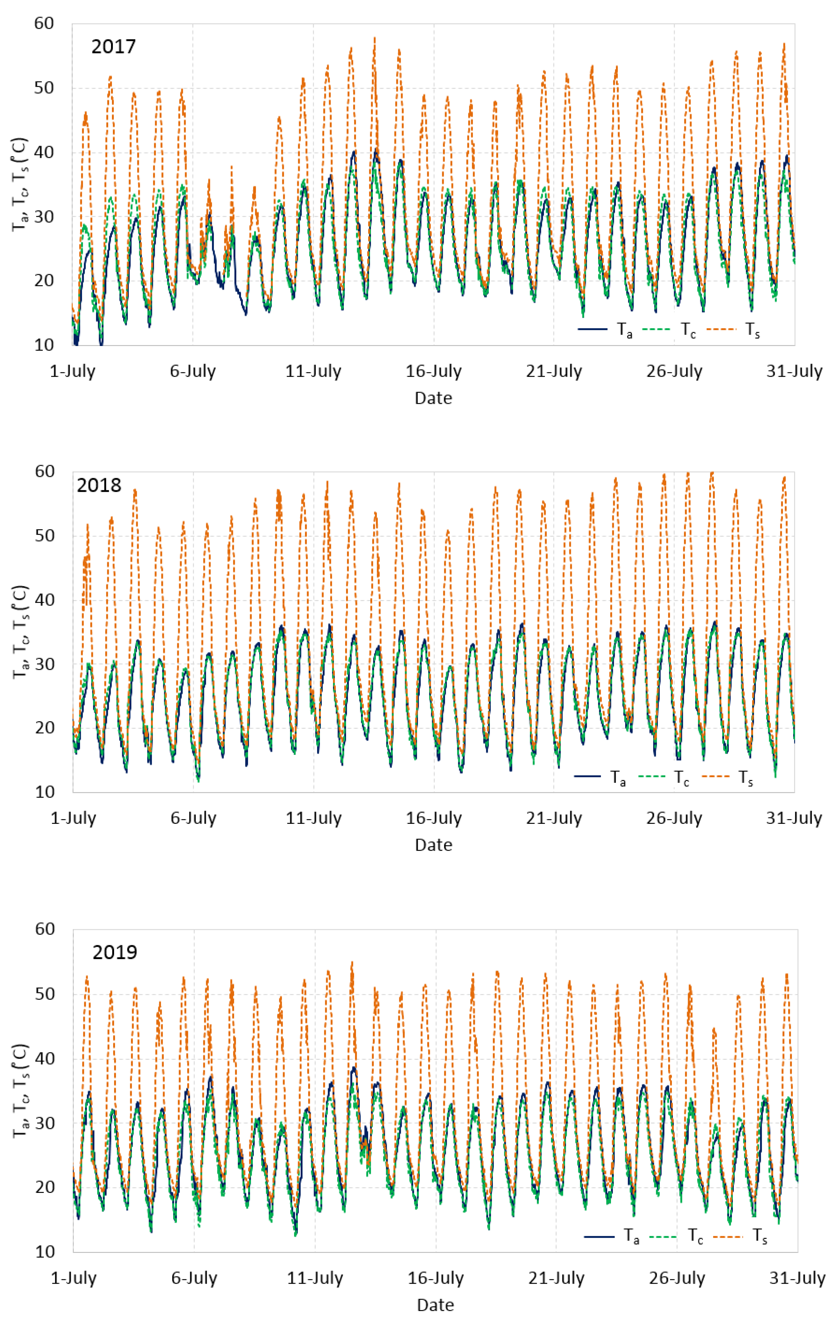
3.1. Weather Conditions and Reference Evapotranspiration

Table 1. Almond growing season monthly meteorological means or totals for the experimental period (2017–2019), and 30-year means of T_{a mean} and rainfall in brackets.

	Ta mean	RHmin	u2	S	Rainfall *	ETo
	(°C)	(%)	(m s−1)	(MJ m−2 d−1)	(mm)	(mm d−1)
2017
March	9.5 (9.3)	40.1	3.1	18.1	60.0 (26.6)	2.8
April	12.2 (11.6)	34.2	2.7	22.3	22.3 (39.3)	3.8
May	16.7 (15.6)	28.6	2.7	26.1	8.9 (40.8)	5.3
June	22.9 (21.0)	20.7	2.9	29.0	0.0 (24.4)	6.4
July	24.2 (24.6)	19.5	2.4	27.7	25.4 (7.0)	7.0
August	23.7 (24.2)	25.5	2.5	23.3	6.1 (9.7)	5.8
September	19.3 (19.2)	24.4	2.4	20.7	1.2 (32.4)	4.8
October	15.6 (14.3)	32.7	1.7	14.7	8.4 (32.6)	2.6
November	8.2 (8.6)	33.6	2.1	10.5	10.7 (32.8)	1.5
2018
March	8.2 (9.3)	47.9	5.4	15.2	63.5 (26.6)	2.5
April	11.5 (11.6)	40.0	3.7	19.7	19.9 (39.3)	3.4
May	14.6 (15.6)	35.6	2.4	24.7	64.0 (40.8)	4.3
June	19.6 (21.0)	33.2	2.4	25.3	46.4 (24.4)	5.3
July	24.1 (24.6)	16.1	2.5	28.7	0.0 (7.0)	7.3
August	24.4 (24.2)	24.7	2.6	24.0	15.3 (9.7)	6.3
September	20.3 (19.2)	37.7	2.0	18.7	99.3 (32.4)	3.9
October	13.4 (14.3)	42.9	2.4	13.3	23.3 (32.6)	2.5
November	9.1 (8.6)	63.2	3.1	8.1	69.2 (32.8)	1.2
2019
March	9.3 (9.3)	29.9	2.6	18.8	18.0 (26.6)	3.0
April	10.5 (11.6)	44.8	3.5	18.5	123.7 (39.3)	3.0
May	16.0 (15.6)	29.1	2.7	26.4	16.3 (40.8)	4.9
June	20.5 (21.0)	20.4	2.8	29.2	0.0 (24.4)	6.7
July	24.7 (24.6)	20.6	2.8	27.5	0.0 (7.0)	7.4
August	23.7 (24.2)	21.6	2.2	24.5	17.5 (9.7)	6.2
September	19.6 (19.2)	37.5	2.6	17.4	38.3 (32.4)	4.0
October	15.0 (14.3)	38.8	2.4	13.9	18.9 (32.6)	3.1
November	9.2 (8.6)	56.4	5.0	8.8	38.5 (32.8)	1.8

T_{a mean} is mean air temperature, RH_min is minimum relative humidity, u₂ is 2 m wind speed over a grass reference crop, S is global solar radiation, * is total monthly precipitation, ET_o is the FAO56 PM daily reference evapotranspiration.

shows a summary of monthly meteorological parameters at an experimental site during the 2017, 2018 and 2019 almond growing seasons and compares mean air temperature and rainfall data with long-term averages (in brackets). In general terms, the three growing seasons were representative of the 30-year means meteorological conditions in the southeast of Spain. However, records from the weather station mentioned above showed that the mean rainfall in the March through November growing season for the last 30 years is 246 mm. This results in 103 mm more than the 2017 growing season, and 155 and 25 mm less than the 2018 and 2019 seasons, respectively. Cumulative precipitation ranged from 143 in 2017 to 401 mm in 2018, mainly concentrated in spring and fall. Air temperature ranged between 8.2 and 24.7 °C, highlighting that the month of June was around 3 °C warmer in 2017 compared to 2018 and 2019. The daily wind speeds and solar (shortwave) radiation were typical values for the experiment site. Monthly averages of wind speed at 2 m of height ranged between 1.7 and 5.4 m s⁻¹ and solar radiation between 8.1 and 29.2 MJ m⁻² d⁻¹.

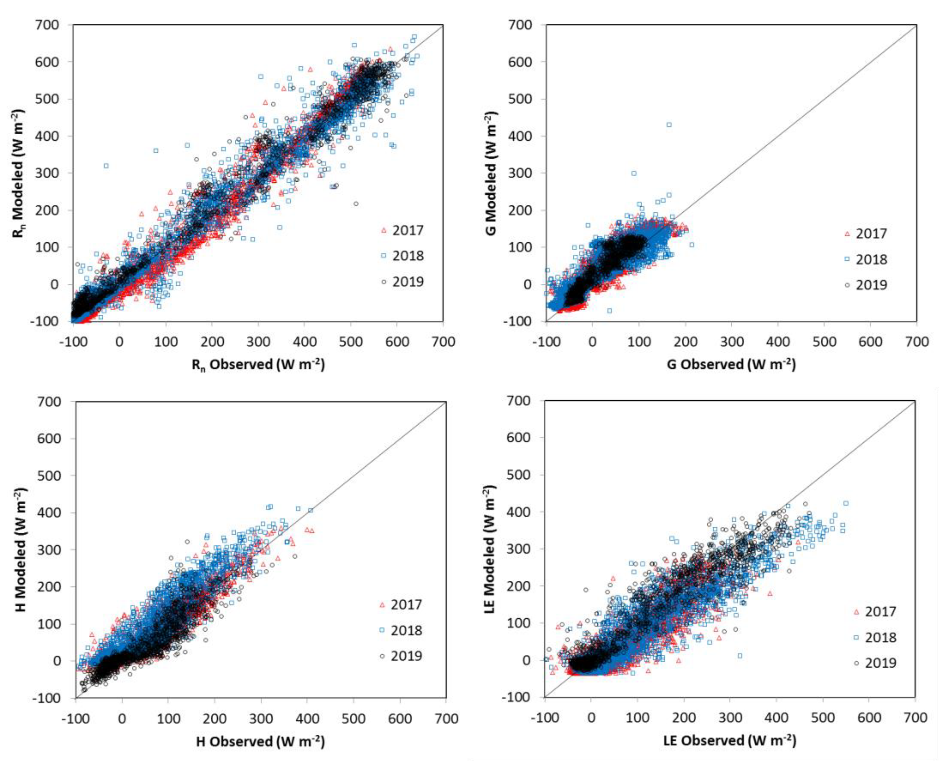
3.2. Energy Balance Closure

Prior to the assessment of the latent heat flux outputs through the STSEB, by comparison to eddy-covariance measurements, the lack of closure in the surface energy balance from the gathered flux data was evaluated. Hourly values of all fluxes were calculated by averaging stored 15 min data. Figure 5 shows the linear regression between the sum of turbulent fluxes (H + LE) and the available energy (R_n-G). Similar results were obtained for the three seasons, with a lack of closure around 20%. These results are in agreement with imbalance values traditionally reported in a variety of croplands and climates [48]. In one of the very few analyses of energy balance closure on almond orchard plantations, Stevens et al. [18] reported a closure of 0.87 from half-hourly eddy-covariance flux data in a mature almond orchard in South Australia.

This analysis of the energy balance closure supports the experimental setup, and particularly the mounting height for the EC instrumentation. Literature is not conclusive about the method to be followed for facing the imbalance [38]. The residual (RE) technique was selected in this work, assuming correct H measures and the underestimation of LE, based on previous results in similar irrigated croplands under advection [30,49].

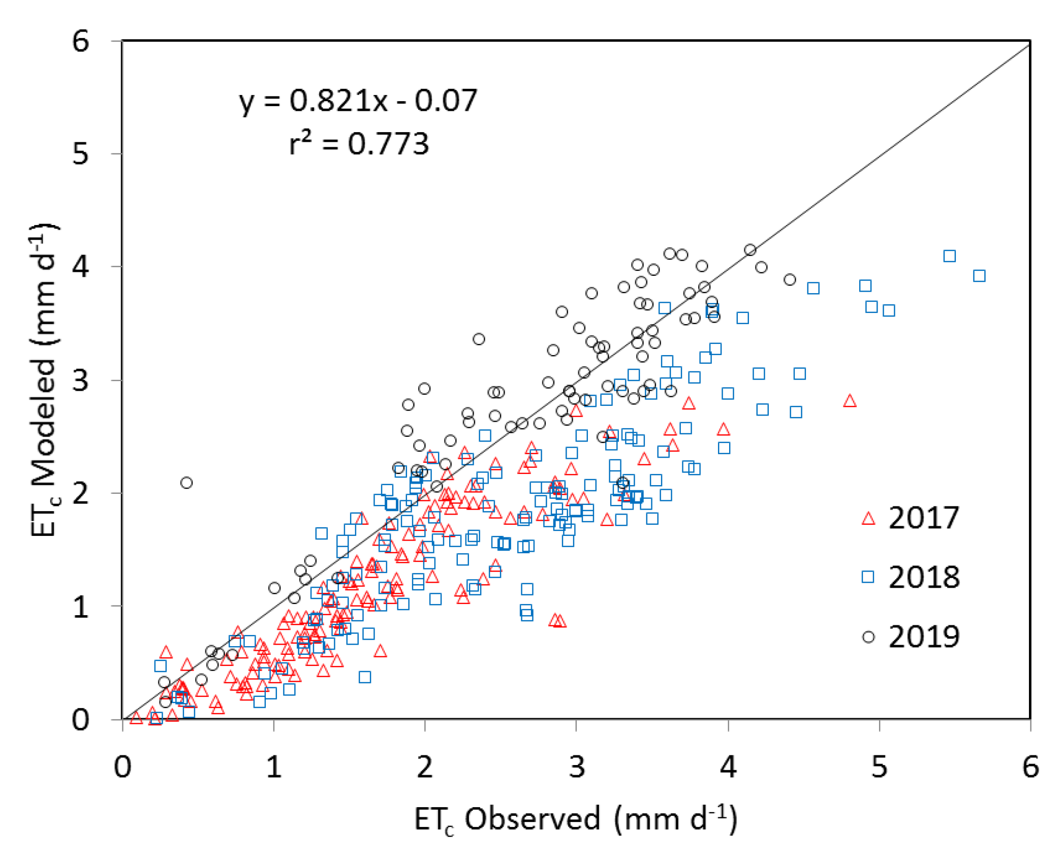
3.3. Assessment of the STSEB Model

Once corrected from atmospheric and emissivity effects, soil and canopy temperatures were used as inputs in the set of Equations (1)–(11), together with meteorological data from the weather station and the ancillary biophysical parameters monitored during the experiment. Near 8000 hourly observations were available for the assessment of the STSEB model outputs.

Plots in Figure 6 show the comparison between modeled and observed hourly fluxes, and the main statistical results of these linear regressions are listed in

Table 2. Statistics of the linear regressions between modeled and observed hourly values of the surface energy fluxes: net radiation (R_n), soil heat flux (G), sensible heat flux (H) and latent heat flux (LE).

Year (N)		Slope	Intercept (W m−2)	r2	Bias (W m−2)	RMSE * (W m−2)
2017 (2526)	Rn	1.03	−7	0.975	−4	34
	G	1.03	14	0.834	15	31
	H	0.87	20	0.892	13	29
	LE	0.82	−10	0.828	−22	44
2018 (3675)	Rn	0.98	5	0.975	2	36
	G	0.80	15	0.815	14	32
	H	0.99	24	0.872	24	37
	LE	0.79	−7	0.871	−23	48
2019 (1568)	Rn	0.98	16	0.982	13	35
	G	1.12	15	0.890	16	25
	H	0.83	7	0.827	1	31
	LE	0.88	14	0.915	3	40

* Error values are shown with two significant figures in order to allow for further analysis and comparisons. r²: coefficient of determination. Biased estimator: Bias = ${\displaystyle \sum }_{\mathrm{i}=1}^{\mathrm{n}}\left(\mathrm{Pi}-\mathrm{Oi}\right)/\mathrm{n}$. Root mean square difference: RMSE = ${\left[{\displaystyle \sum }_{\mathrm{i}=1}^{\mathrm{n}}{\left(\mathrm{Pi}-\mathrm{Oi}\right)}^2/\mathrm{n}\right]}^{1/2}$. Where Pi and Oi are the predicted and observed values, respectively.

. Uncertainty values ranging from ±30 to 40 W m⁻² were obtained for modeled R_n, G and H fluxes, and between ±40 and 50 W m⁻² for LE. No significant differences were observed in the performance of the model for the 3 years in terms of R_n or G. However, a slight overestimation of H, and a consequent underestimation of LE, was obtained for the 2017 and 2018 seasons. This was not the case for the 2019 data, when an RMSE = ±40 W m⁻² with a negligible bias was observed. The reason could be the rise in the EC instrumentation for the 2019 experiment, together with the decrease in the footprint mentioned above (see Figure 3). In terms of hourly ET_c, negligible bias was observed in 2019, whereas the underestimation for 2017 and 2018 resulted in 0.03 mm h⁻¹. A common RMSE = 0.06 mm h⁻¹ was obtained for the 3-year dataset.

These results are in agreement with previous evaluations of the STSEB approach in maize [29] or vineyard [30], and give confidence to the model outputs of ET_c, as representative and feasible estimates of the actual crop evapotranspiration for the drip-irrigated young almond orchard, as well as its partition into soil evaporation and canopy transpiration.

Daily values of ET_c were obtained by adding the hourly data. Figure 7 now shows the linear regression between ET_c values computed from the STSEB model and observed (measured) with the EC system, for near 400 days in total. The main statistical results are included in

Table 3. Statistical analysis of the comparisons shown in Figure 7. Results corresponding to the comparison with direct EC measurements (not corrected) are shown in brackets.

	N	Slope	Intercept (mm d−1)	r2	Bias (mm d−1)	RMSE (mm d−1)
2017	154	0.75 (0.50)	−0.07 (0.3)	0.829 (0.500)	−0.5 (−0.5)	0.6 (0.9)
2018	161	0.71 (0.62)	0.02 (0.3)	0.775 (0.581)	−0.7 (−0.6)	0.9 (1.0)
2019	80	0.89 (0.69)	0.4 (0.6)	0.840 (0.725)	0.08 (−0.3)	0.4 (0.7)

. An overall good agreement was obtained between the STSEB outputs and observed ET_c measurements, with an average uncertainty below ±1.0 mm d⁻¹. In a detailed analysis per year, underestimation values of 0.5 and 0.7 mm d⁻¹ were observed for the 2017 and 2018 campaigns, respectively, being mainly responsible for the ±0.6 and ±0.9 mm d⁻¹, respectively. This systematic deviation disappears for the 2019 data, with an average error of ±0.4 mm d⁻¹. This behavior was previously observed for instantaneous values of LE on an hourly scale and might be a consequence of the improvement in the experimental deployment for this 2019 season, as mentioned above. Moreover, both the sonic anemometer and the gas analyzer were recalibrated at the beginning of the 2019 campaign, and this might have a positive effect on the ground EC measurements.

Uncertainty values ranging from ±0.4 to ±1.1 mm d⁻¹ have been reported in the literature, in modeled ET_c using two-source energy balance approaches combined to local radiometric temperatures, when comparing to lysimeter or eddy-covariance measurements, in a variety of crops (Table 4).

As far as the authors are concerned, the assessment of this technique applied to almond orchards has not been explored before using ground measurements of radiometric temperature components. Some recent works focused on the estimation of ET_c in almond orchards using remote sensing approaches and satellite or flight images. Bellvert et al. [9] reported an RMSE value of 0.74 mm d⁻¹ using the combination of an ET-based model and thermal-based plant water status indicators applied to Landsat-8 and airborne imagery. These authors tested their results against eddy-covariance data. Also based on Landsat-8 images, Ref. [50] evaluated the performance of three remote-sensing-based ET models using ground data derived using surface renewal technique as a basis. RMSE values ranging from 0.9 mm d⁻¹ to 1.6 mm d⁻¹ were reported by these authors, with r² ranging from 0.74 to 0.82.

Table 4. Summary of the statistics for some assessments of the two-source energy balance scheme combined with radiometric surface temperatures, reported in the literature over different croplands, using eddy-covariance (LE) or weighing lysimeter measurements (Hourly and Daily ET_c) as a basis.

	Model	Crop	N Days	LEi (W m−2)		Hourly ETc (mm h−1)		Daily ETc (mm d−1)
				Bias	RMSE	Bias	RMSE	Bias	RMSE
Kustas et al. [22]	TSEB	Cotton	5	5	47	-	-	-	-
Sánchez et al. [29]	STSEB	Maize	50	−6	51	-	-	-	-
Sánchez et al. [51]	STSEB	Sorghum	73	-	-	−0.004	0.14	−0.3	1.0
Colaizzi et al. [27]	TSEB	Cotton	170	5/−3	67/86	-	-	0.2/−0.1	0.6/1.1
Sánchez et al. [52]	STSEB	Sunflower	61	-	-	0.03	0.16	0.05	1.0
		Canola	90	-	-	0.04	0.20	0.18	1.1
Sánchez et al. [53]	STSEB	Wheat	138	-	-	−0.010	0.11	−0.18	0.8
Song et al. [31]	TSEB	Maize	98	12/41	50/59	-	-	0.2/−0.6	0.4/0.7
		Cotton	28	−33/21	95/166	-	-	-	-
Sánchez et al. [30]	STSEB	Vineyard	288	−10	53	-	-	–0.04	0.6

Table 4. Summary of the statistics for some assessments of the two-source energy balance scheme combined with radiometric surface temperatures, reported in the literature over different croplands, using eddy-covariance (LE) or weighing lysimeter measurements (Hourly and Daily ET_c) as a basis.

	Model	Crop	N Days	LEi (W m−2)		Hourly ETc (mm h−1)		Daily ETc (mm d−1)
				Bias	RMSE	Bias	RMSE	Bias	RMSE
Kustas et al. [22]	TSEB	Cotton	5	5	47	-	-	-	-
Sánchez et al. [29]	STSEB	Maize	50	−6	51	-	-	-	-
Sánchez et al. [51]	STSEB	Sorghum	73	-	-	−0.004	0.14	−0.3	1.0
Colaizzi et al. [27]	TSEB	Cotton	170	5/−3	67/86	-	-	0.2/−0.1	0.6/1.1
Sánchez et al. [52]	STSEB	Sunflower	61	-	-	0.03	0.16	0.05	1.0
		Canola	90	-	-	0.04	0.20	0.18	1.1
Sánchez et al. [53]	STSEB	Wheat	138	-	-	−0.010	0.11	−0.18	0.8
Song et al. [31]	TSEB	Maize	98	12/41	50/59	-	-	0.2/−0.6	0.4/0.7
		Cotton	28	−33/21	95/166	-	-	-	-
Sánchez et al. [30]	STSEB	Vineyard	288	−10	53	-	-	–0.04	0.6

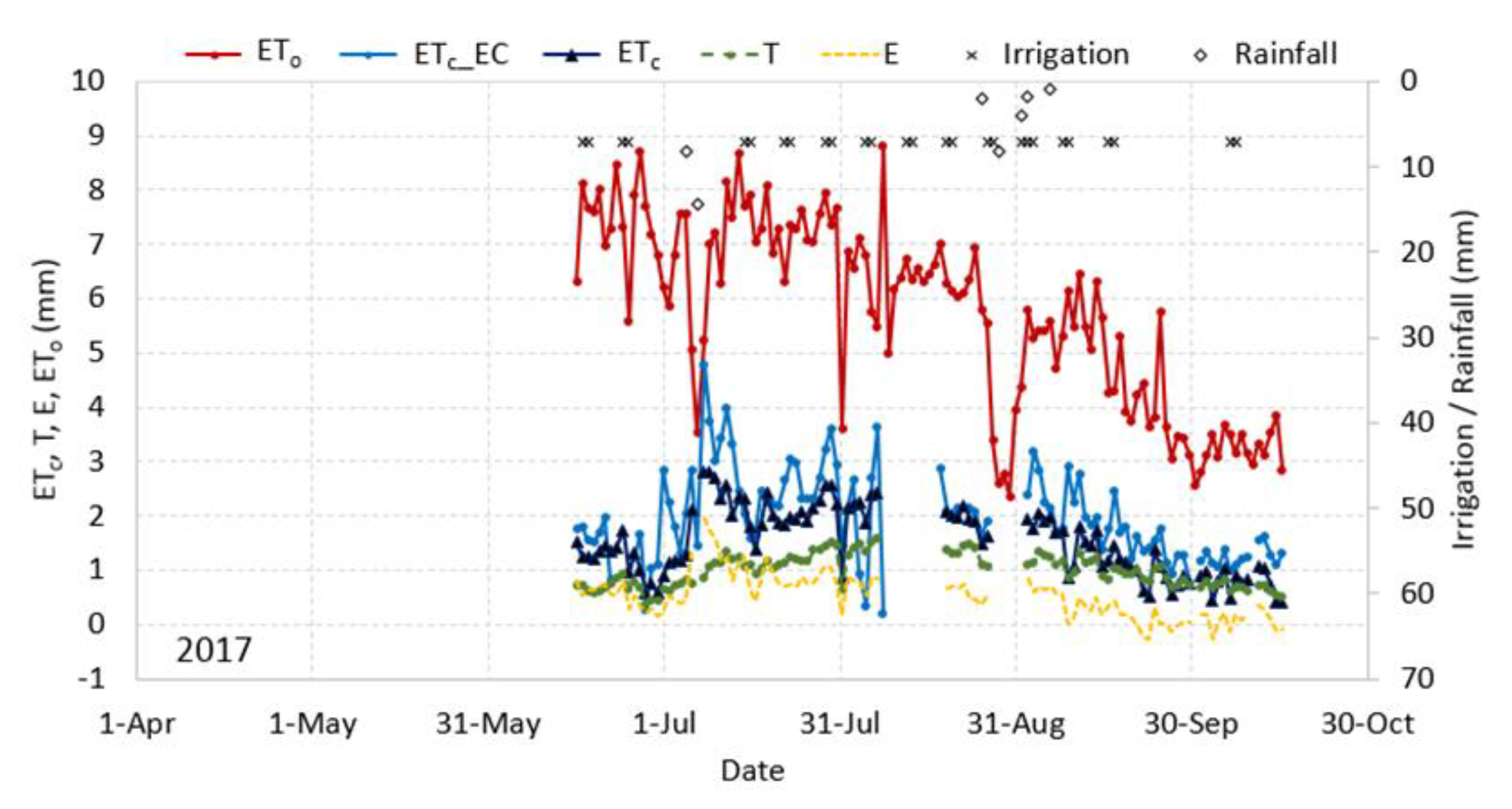
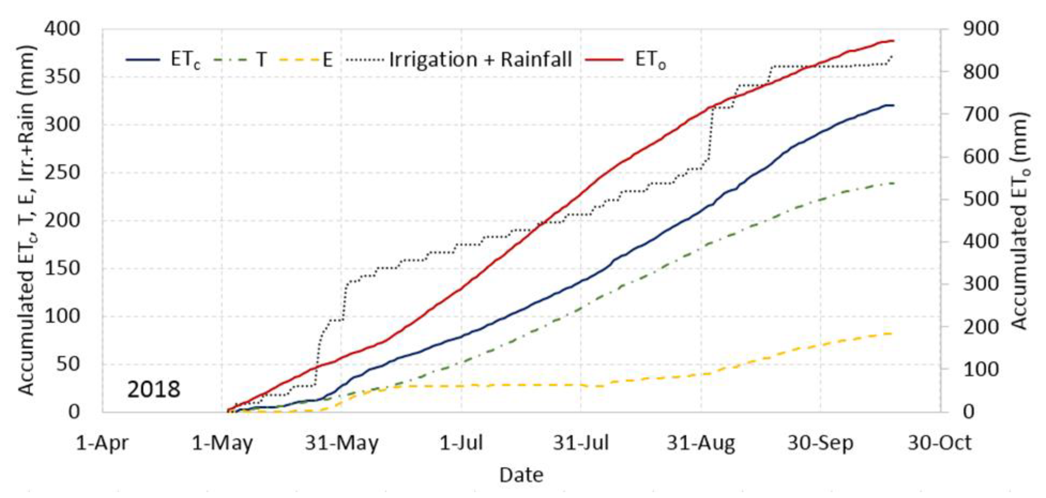
3.4. Crop Evapotranspiration Estimates

Figure 8 shows the evolution of STSEB-modeled daily ET_c, together with its separated components E and T for the 3-year dataset. Values of registered ET_o, as well as irrigation plus rainfall amounts, are superposed to the plots for a better understanding of the ET_c, T and E behavior. Note that some days/periods must be excluded from a further analysis of the crop coefficients due to the adverse weather conditions affecting the K_cb and K_c trends. This is the case for April and September 2019, as well as mid-May to Mid-June and September 2018.

Within the first three years after planting (2017 and 2018 campaigns), ET_c values rarely overtook the 2 mm d⁻¹ consequence of the low canopy cover of the very young almond trees (maximum f_c values of about 21% and 35% for 2017 and 2018, respectively). Only after some rain or remarkable irrigation did ET_c rise above this limit set by the high evaporation contribution (see Figure 8). For these two seasons, ET_c increased after flowering caused by the leaf growth facilitated by the helpful spring and early summer temperatures, and rising ET_o values. Peak ET_c was reached along July and August, coinciding with the end of Stage III (dry matter accumulation in the kernel) [14] (see

Table 5. Monthly mean values of crop evapotranspiration (ET_c), canopy tree transpiration (T), soil evaporation (E), and crop coefficients (K_c, K_cb, and K_e) for the 3 almond growing seasons of the experiment. The number of days (values) used per month (N) is also listed.

	N	ETc	T	E	Kc	Kcb	Ke
		(mm d−1)	(mm d−1)	(mm d−1)
2017
May	-	-	-	-	-	-	-
June	15	1.18	0.66	0.53	0.17	0.09	0.07
July	29	2.01	1.10	0.92	0.28	0.15	0.12
August	20	1.96	1.32	0.64	0.32	0.22	0.10
September	28	1.27	1.01	0.26	0.27	0.21	0.05
October	14	0.77	0.68	0.09	0.24	0.21	0.03
2018
May	22	0.53	0.49	0.04	0.14	0.11	0.02
June	20	1.51	1.25	0.26	0.25	0.20	0.05
July	30	1.87	1.85	0.02	0.26	0.25	0.00
August	17	2.33	2.01	0.33	0.40	0.35	0.06
September	-	-	-	-	-	-	-
October	-	-	-	-	-	-	-
2019
May	25	2.5	1.44	1.07	0.5	0.29	0.21
June	29	2.82	2.00	0.82	0.42	0.3	0.12
July	30	3.03	2.48	0.55	0.41	0.34	0.08
August	19	3.33	2.54	0.78	0.48	0.37	0.12
September	-	-	-	-	-	-	-
October	-	-	-	-	-	-	-

). Four growing seasons after planting, for the 2019 campaign, canopy density and fraction of ground cover have increased (maximum f_c value of 42%). As a consequence, ET_c values are regularly over 3.0 mm d⁻¹ in Stage III. A similar trend is observed in terms of isolated canopy transpiration, for which the effect of rainfalls diminishes, and a better relationship with biophysical parameters is then expected.

Table 5 summarizes the monthly mean values for the three growing seasons. Evaporation is highly dependent on rainfall, with mean values generally lower than 0.6 mm d⁻¹ when no rain is registered. Transpiration is less sensitive to rainfall, and mean values increase is linked to the canopy cover gain from the 2017 to 2019 seasons. The maximum mean values reached are 1.3, 2.0, and 2.5 for August 2017, 2018, and 2019, respectively.

Seasonal water use could not be accurately determined in this experiment since the study periods did not cover the full growing season (March–October). However, accumulated values were estimated for the available datasets. As an example, the plot in Figure 9 shows the evolution of the accumulated ET_c, together with separated T and E, for the 2018 season. A total ET_c of 321 mm was obtained, with 26% (82 mm) corresponding to soil evaporation and 74% (239 mm) to canopy transpiration. A mean value of ET_c = 1.9 mm d⁻¹ resulted for the study period in 2018. Accumulated irrigation plus rainfall summed 374 mm, which is a 16% over total ET_c. For the same period, accumulated ET_o resulted 874 mm, which means a ratio ET_c/ET_o = 0.37 for the 2018 season. This average ratio was increasing from 0.22 in 2017 to 0.61 in 2019, mainly because tree canopies expanded from 10% to 42% of vegetation fractional cover during the experimental period. A similar trend was observed for the mean value of ET_c, rising from 1.5 mm d⁻¹ in 2017 up to 3.4 mm d⁻¹ in 2019.

The seasonal water use of an almond orchard depends on the fraction of canopy cover and the evaporative demand. There is a lack of studies focused on measuring water requirements of young almond trees. Stevens et al. [18] reported a seasonal ET_c of 1430 mm for a high-yielding mature almond orchard (cv. Nonpareil) in South Australia. In an experiment carried out in Córdoba (Spain), Ref. [11] used weighing lysimeter and sap flow measurements to determine the water use of a young almond orchard (cv. Guara). Maximum transpiration values were reached mid-July and maximum transpiration coefficient values increased every year as canopy cover expanded. Goldhamer and Fereres [54] reported seasonal mature almond trees’ (cvs. Nonpareil and Monterey) ET_c ranging between 1100 and 1350 mm in a long-term field study conducted in western Kern County, California. Bellvert et al. [9] conducted an experiment aiming at estimating seasonal ET_c and crop coefficients for an 18-year-old almond orchard (cv. Nonpareil) located in Central Valley (California). These authors reported ET_c increasing sharply from early March to mid-July, when maximum values of 8.5 mm d⁻¹ were achieved, and then dropping until the end of the season.

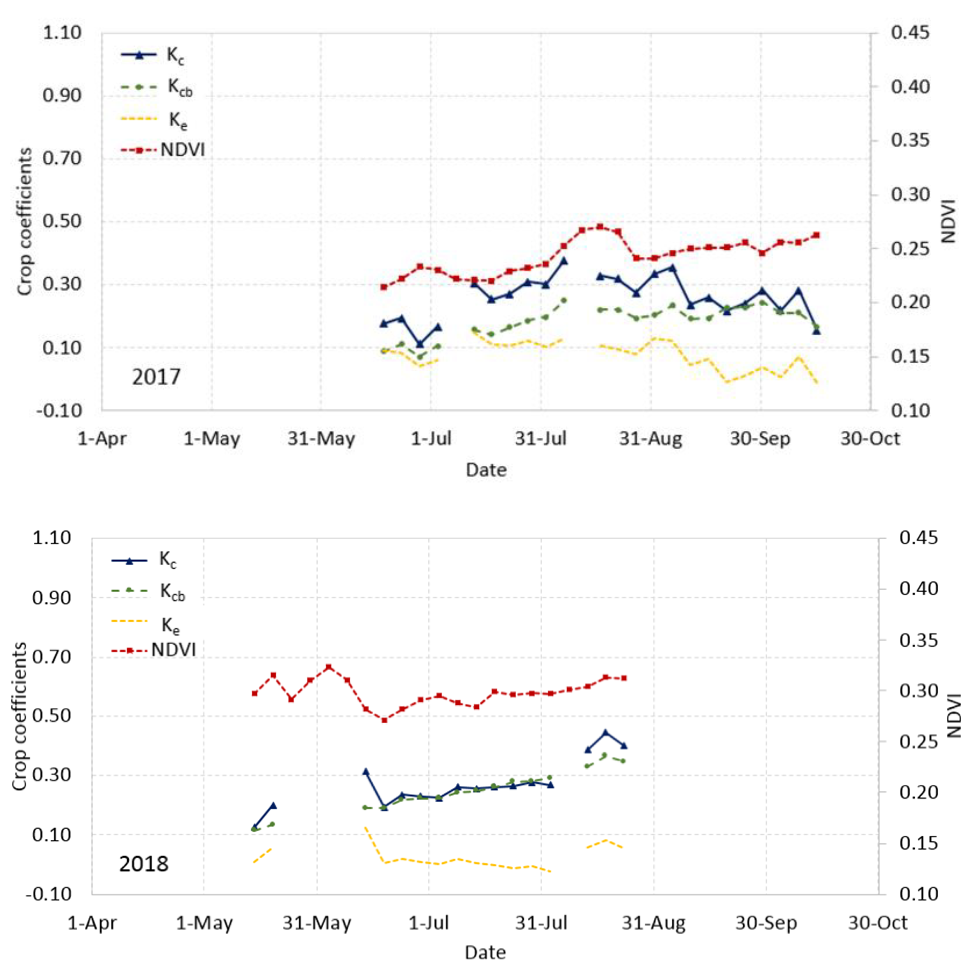
3.5. Crop Coefficients for Young Almond Trees

Figure 10 plots the curves of K_c, calculated as the ratio of the modeled ET_c/ET_o, together with the dual crop coefficients K_e and K_cb, calculated as the ratios E/ET_o and T/ET_o, respectively. To avoid the scatter produced by irrigation events, crop coefficient values are presented as 5-day averages [53]. Time frames of 2 days after every rain event with >5 mm were discarded from this analysis to avoid disruption into the crop coefficient trends.

As mentioned above, K_e values around or lower than 0.10 were maintained, except for those humid periods with a significant rain amount. This is for instances such as the case of mid-May to mid-June and September 2018, or the first weeks in May and last weeks in August 2019. Although humid and rainy weather conditions affect this analysis, the overall trend is that K_cb values increase from May, peak by the end of August, and start dropping entering September. Moreover, June–July were identified as the hottest and driest months, with the highest evaporative demand, for the three growing seasons, whereas the maximum average values of K_c and K_cb were reached in August. Table 5 includes the monthly mean values of these crop coefficients for the full dataset. To better illustrate this trend in the crop coefficients, Figure 11 plots a separate analysis per year.

Average mid-season K_cb, K_{cb mid}, resulted in 0.19, 0.30, and 0.36, for the 2017, 2018, and 2019 seasons, respectively, whereas mid-season K_c values, K_{c_mid}, of 0.30, 0.33, and 0.45 were obtained for the 2017–2019 experiments, respectively. Differences in K_c values between years for the same period are directly related to data availability and the main factors affecting crop coefficients relative to different almond growth stages. When f_c values are low, the variability of K_c is mainly linked to soil evaporation (differences explained below). For instance, mean K_c in July of 2017 and 2018 resulted 0.28 and 0.26, respectively. A higher value in then obtained in 2017, although f_c is significantly lower than in 2018. This is explained by a much higher value of K_e in 2017 compared to that in 2018. As growing season progressed, the canopy cover expanded, becoming the main factor affecting K_c values. Obviously, this is more evident in the K_cb values (tree transpiration component), which increased throughout the crop cycle (May–August) and every year (from 2 to 4 years of trees age) as f_c values became higher.

Differences in K_e values between years observed in Figure 11 and Table 5 are explained as follows. As f_c increases from 2017 to 2019, a reduction in the contribution of the soil to the total ET_c, and then a decrease in average K_e values, are expected as long as both environmental conditions and irrigation scheduling remain similar. However, the opposite trend is observed in Figure 11 when comparing 2018 and 2019, highlighting that irrigation scheduling plays a key role at this K_e behavior. As mentioned above, 2018 was a rainy year (over the average), with a rainfall amount about 100 mm higher than 2017 or 2019 for the same May–August period. For this reason, irrigation water supply in 2019 almost doubled that in 2018, for the same period (see plots in Figure 8), and soil evaporation became larger. Moreover, a few precipitation events occurred by the end of April in 2019 with a significant rainfall accumulation over 120 mm. This has an impact on the large K_e values observed in Figure 10 for the first weeks in May, as well as the corresponding monthly average in Figure 11 and Table 5. Note that the K_c trend in 2019 also accounts for this distinctive feature. It must be restated that those days with rainfall events were excluded from this analysis.

The error bars included in Figure 11 provide an insight into the statistical significance of the monthly averages shown. Accounting for these uncertainties, K_e values could be set to zero in 2018 (except August), as well as the period September–October in 2017. Uncertainties in mean K_cb are lower, highlighting a higher precision in the modeled transpiration component.

Some studies have reported E values accounting for 24% of ET_c in drip-irrigated mature almond orchards during the growing season [55]. This ratio depends on how the irrigation systems are used and managed (i.e., the frequency of irrigation events and irrigation depth applied). Using a micro-sprinkler system, [9] estimated an average of 16%.

To our knowledge, there is a lack of studies focused on producing crop coefficients for young almond trees. In the experiment by [11], maximum transpiration values were reached mid-July and maximum transpiration coefficient values were observed to increase every year as canopy cover expanded. The maximum K_cb of 0.5 and 0.6 was reached when trees were three and four years old and maximum f_c values were 35 and 50%, respectively. These values are in agreement with our findings, since a maximum K_cb close to 0.4 is also obtained for our 4-year-old almond trees in 2019. This small difference could be explained by a lower f_c value in our study (Figure 2). Although these authors did not show K_c values, they assumed that soil evaporation can range between 10 and 15% of ET_c, resulting in maximum K_c values of 0.57 and 0.69, which is also in agreement with the maximum K_c values obtained in our study. Later, in the same lysimeter facility, López-López et al. [19] reported average mid-season K_cb values of 0.55, 0.68 and 0.91 in three seasons (6–9 years after planting), with maximum f_c values ranging from 0.55 to 0.59. These authors proposed a K_cb between 0.9 and 1.05 for fully mature almond orchards, with a f_c of 0.75.

Another of the scarce studies on young almond trees was conducted by [12] in a four-year-old almonds orchard in southwest Spain. ET_c was measured using four drainage lysimeters. Almonds located in these lysimeters were irrigated at 130% of a theoretical ET_c. The K_c values changed from 0.4 at the beginning of the irrigation period to a maximum of 1.1 during the maximum evaporative demand period. These values are significantly higher than those obtained in the present paper. Unfortunately, these results are based on only one season of data and they did not show f_c values.

Other studies have reported mid-season K_c values for fully mature almond orchards with high f_c values (>70%). In this regard, [14] showed the monthly K_c values reported by Girona (2006) (technical report in Spanish) based on the soil water balance approach. Girona reported maximum K_c values of 1.05 in August. Stevens et al. [18] reported a maximum K_c of 1.1 for a high-yielding almond orchard (cv. Nonpareil) in South Australia. Bellvert et al. [9] reported maximum values of K_c of 1.3 at full development, after each irrigation event, with nominal values ranging from 0.9 to 1.1. Obviously, these K_{c mid} values are higher to those obtained in our study since they correspond to mature trees with f_c values greater than 70%.

Recently, a review article has been published by [10] aiming at updating single and dual crop coefficients for fruit trees and vines. These authors reported indicative standard values of mid-season K_c and K_cb of 0.45 and 0.40, respectively, with a range of ±10% for almond trees with low density and an f_c value of 30–40%. Both K_{c mid} and K_{cb mid} values are in agreement with those obtained in our study when trees were 4 years old.

3.6. Relationships between Crop Coefficients and Biophysical Variables

Plots in Figure 10 superpose the evolution of the NDVI extracted from the temporal series of the satellite images from the constellation Sentinel-2A/B + Landsat 8 (SpiderWebGis©) during the 2017–2019 growing seasons. Values correspond to an average of 5 × 5 pixels. NDVI captures the almond orchard growth and describes the crop development for the study periods in 2017 and 2018. However, for the 2019 season, a descending trend in the NDVI is observed during May–June, while the K_cb remains unaltered in a flat constant value of 0.30. The reason was the green weeds covering the inter-row soil in the parcel that had not been removed at the beginning of this season, and that were contributing to increase the reflectance response in the near infrared leading an increase in the pixel NDVI, masking the real behavior of the almond tree canopy. This shows the limitation of vegetation indices such as NDVI to monitor the crop growing when dealing with fruit orchards when weeds are not correctly managed.

Figure 12 shows the linear fit between the crop coefficients and the NDVI for the complete dataset. When data from the three growing seasons are treated together, a good correlation is obtained between K_cb and NDVI, with a determination coefficient of r² = 0.775. However, although spring dates affected by the non-removed ground green weeds were excluded from this linear regression, a larger scatter is observed for the relation K_c-NDVI, with a value of r² = 0.441.

Most of the studies that review the linear and polynomial relationships to determine K_cb from NDVI and other vegetation indices [44,45] show a variety of functions for herbaceous crops, but few can be found about almond trees and other orchards [56,57]. This is due to the difficulty of measuring the transpiration of this complex cover that is partially covered, frequently under water-stress, and with part of the soil exposed to evaporation. The results provided in our almond orchard from a previous local calibrated relationship for vineyard [46] show a value of K_{cb mid} = 0.37 for the year 2019 compared to the 0.36 in this work. Note that the remote sensing data in both experiments were processed in the same way, so they are comparable (atmospheric correction, observing and illumination geometry and pixel size), and similar setup and processing of data from flux towers were conducted. The differences observed are likely due to crop phenology and management. The initial crop stage in almond is flowering with none to very low transpiration in contrast to other crops such as vines for which it is initiated with emerging leaves. These models can be compared with caution to other approaches using intermediate biophysical variables such as intercepted radiation to estimate K_cb from NDVI [9], due to important differences in crop management with some green cover below almonds at initial crop development and higher values of the basal crop coefficient. Nevertheless, by applying the model developed by [9] to this experiment, a value of 0.38 resulted for the middle stage.

Some authors suggest the fraction of ground covered by vegetation (f_c) as a better estimator of the K_cb coefficient [58]. Plots in Figure 12 also depict the K_cb versus f_c values registered during the 3-year dataset. A better fitting is now obtained, with a lower scatter and a higher correlation coefficient over 0.90. However, a poorer dependence is observed between K_c and f_c (see Figure 12), with a value of r² = 0.618 (once the dates affected by weeds were excluded). This was expected since the vegetation fractional cover is a biophysical parameter referring only to the tree canopy, and then not accounting for the soil, whereas K_c includes the soil evaporation component through K_e.

Although crop transpiration responds physiologically to the daily fraction of photosynthetically active radiation intercepted by the canopy (fIRd), this variable is well correlated to f_c. Espadafor et al. [11] found a good relationship between transpiration and f_c, with a ratio of 1.2, very similar to the 1.0 obtained in the present work. However, these authors advised that this ratio should not be considered fixed. Using the fIRd, [11] extrapolated a value of K_cb around 1.0 to mature orchard conditions.

The validity of these equations for mature almond orchard trees will be assessed in future works, using data gathered in further experimental campaigns. The operational application and robustness of this VI-K_cb approach for different varieties and under different environmental conditions will be also explored. Further measurements of f_IPAR will allow a for comprehensive analysis of the transpiration response to this parameter and its connection to f_c and NDVI in almond orchards.

4. Conclusions

Despite the experimental limitations in young orchards, this work shows the feasibility of the STSEB approach, combined to radiometric temperature measurements, to capture the surface energy flux patterns of a drip-irrigated young almond orchard, with average errors below 50 W m⁻² for instantaneous fluxes. Crop evapotranspiration is calculated with an average accuracy of 0.06 mm h⁻¹ and 0.6 mm d⁻¹ on hourly and daily scales, respectively. These results are based on data gathered in a 3-year experiment, starting the second year after planting, and then covering a wide range of environmental and growing stage conditions, which reinforces the assessment. The challenging conditions of this young almond orchard did not diminish the performance of the two-source approach previously reported in a variety of crops.

Furthermore, the potential of a two-source scheme to separate soil and canopy energy balances brings new insights in the partition of soil evaporation and canopy transpiration in almond orchards and might be the perfect complement to the traditional irrigation scheduling based on soil water balances. Moreover, this accurate quantification of the evaporation/transpiration components becomes critical in irrigation strategies or decisions on the irrigation system itself (surface drip, subsurface drip, sprinklers, etc.).

The crop coefficients derived for the 3-year growing seasons, with vegetation cover fractions peaking as much as 42% in 2019, add to those reported in the very few studies on young almond orchards. Values of single and dual crop coefficients plotted and listed in this work contribute to fill this lack of data focusing on the early stages of almond tree development. Moreover, the good correlation observed between crop coefficients and f_c guaranties the prediction of water use for any age almond orchard at least under the conditions of the present study, although this should be further explored.

Finally, this work serves to warn about the use of vegetation indices such as NDVI in remote-sensing-based ET_c modeling when dealing with fruit orchards since the presence of weeds may disrupt their relation to the crop coefficients. Nevertheless, a good correlation was observed in this experiment between crop coefficients and NDVI when surface weeds were correctly managed.

The results in this work are of particular interest in semi-arid areas under water scarcity. Note that our study site is located in a semi-arid area of southeastern Spain, where the land occupancy of almond orchards is experiencing rapid growth, encouraged by the necessity for an adaptation to the water shortage scenarios predicted in the framework of climate change. The findings in this work contribute to enrich our knowledge on young almond orchards under a drip-irrigation management and will benefit further research on water use efficiency and water productivity.

References

1. FAOSTAT. FAO Statistical Database. 2018. Available online: http://www.fao.org/faostat/en/#data/QC (accessed on 26 October 2020).
2. INC. International Nut & Dried Fruit. Nuts & Dried Fruits Statistical Yearbook 2019/2020. 2019. Available online: https://www.nutfruit.org/industry/statistics (accessed on 27 October 2020).
3. MAPA. Anuario de Estadística Agraria. 2019. Available online: https://www.mapa.gob.es/es/estadistica/temas/publicaciones/anuario-de-estadistica/2019/ (accessed on 27 October 2020).
4. Mañas, F.; López-Fuster, P.; López-Urrea, R. Effects of Different Regulated and Sustained Deficit Irrigation Strategies in Almond Production. Acta Hortic. 2014, 1028, 391–394. [Google Scholar] [CrossRef]
5. IPCC. Summary for Policymakers. In Global Warming of 1.5 °C. An IPCC Special Report on the Impacts of Global Warming of 1.5 °C Above Pre-Industrial Levels and Related Global Greenhouse Gas Emission Pathways, in the Context of Strengthening the Global Response to the Threat of Climate Change, Sustainable Development, and Efforts to Eradicate Poverty; Masson-Delmotte, V., Zhai, P., Pörtner, H.O., Roberts, D., Skea, J., Shukla, P.R., Pirani, A., Moufouma-Okia, W., Péan, C., Pidcock, R., et al., Eds.; World Meteorological Organization: Geneva, Switzerland, 2018; p. 32. [Google Scholar]
6. Allen, R.G.; Pereira, L.S.; Raes, D.; Smith, M. Crop Evapotranspiration. Guidelines for Computing Crop Water Requirements, FAO Irrig. Drain. Paper 56; FAO: Rome, Italy, 1998; 300p. [Google Scholar]
7. Pereira, L.S.; Paredes, P.; López-Urrea, R.; Hunsaker, D.J.; Mota, M.; Mohammadi Shad, Z. Standard single and basal crop coefficients for vegetable crops, an update of FAO56 crop water requirements approach. Agric. Water Manag. 2021, 243. [Google Scholar] [CrossRef]
8. Pereira, L.S.; Paredes, P.; Hunsaker, D.J.; López-Urrea, R.; Mohammadi Shad, Z. Standard single and basal crop coefficients for field crops. Updates and advances to the FAO56 crop water requirements method. Agric. Water Manag. 2021, 243, 106466. [Google Scholar] [CrossRef]
9. Bellvert, J.; Adeline, K.; Baram, S.; Pierce, L.; Sanden, B.L.; Smart, D.R. Monitoring crop evapotranspiration and crop coefficients over an almond and pistachio orchard throughout remote sensing. Remote Sens. 2018, 10, 2001. [Google Scholar] [CrossRef] [Green Version]
10. Rallo, G.; Paço, T.; Paredes, P.; Puig, A.; Provenzano, G.; Massai, R.; Pereira, L.S. Updated single and dual crop coefficients for trees and vine crops. Agric. Water Manag. 2021, 250, 106645. [Google Scholar] [CrossRef]
11. Espadafor, M.; Orgaz, F.; Testi, L.; Lorite, I.J.; Villalobos, F.J. Transpiration of young almond trees in relation to intercepted radiation. Irrig. Sci. 2015, 33, 265–275. [Google Scholar] [CrossRef] [Green Version]
12. García-Tejero, I.F.; Hernández, A.; Rodríguez, V.M.; Ponce, J.R.; Ramos, V.; Muriel, J.L.; Durán-Zuazo, V.H. Estimating almond crop coefficients and physiological response to water stress in semiarid environments (SW Spain). J. Agric. Sci. Technol. 2015, 17, 1255–1266. [Google Scholar]
13. López-Urrea, R.; Simón, L.L.; Sánchez, J.M.; Martínez, L.; Valentín, F. Surface energy flux measurements over a drip-irrigated young almond orchard. Acta Hortic. 2021, in press. [Google Scholar]
14. Goldhamer, D.A.; Girona, J. Almond. Crop Yield Response to Water. Irrigation and Drainage; Steduto, P., Hsiao, T.C., Fereres, E., Raes, D., Eds.; Paper no. 66; FAO: Rome, Italy, 2012. [Google Scholar]
15. Fereres, E.; Puech, I. Irrigation Scheduling Guide; A Reference Manual Containing 11 Sections on Irrigation Scheduling; California Department of Water Resources, Office of Water Conservation: Sacramento, CA, USA, 1981; 307p.
16. Girona, J. La respuesta del cultivo del almendro al riego. Vida Rural. 2006, 234, 12–16. [Google Scholar]
17. Sanden, B. Fall Irrigation Management in a Drought Year for Almonds, Pistachios and Citrus. Kern Soil and Water Newsletter, September 2007; University of California Cooperative Extension: Kern County, CA, USA, 2007; Available online: http://cekern.ucdavis.edu/files/64007.pdf (accessed on 28 July 2021).
18. Stevens, R.M.; Ewenz, C.M.; Grigson, G.; Conner, S.M. Water use by an irrigated almond orchard. Irrig. Sci. 2012, 30, 189–200. [Google Scholar] [CrossRef]
19. López-López, M.; Espadafor, M.; Testi, L.; Lorite, I.J.; Orgaz, F.; Fereres, E. Water requirements of mature almond trees in response to atmospheric demand. Irrig. Sci. 2018, 36, 271–280. [Google Scholar] [CrossRef]
20. Kustas, W.P. Estimates of evapotranspiration with a one- and two-layer model of heat transfer over partial canopy cover. J. Appl. Meteorol. 1990, 29, 704–715. [Google Scholar] [CrossRef]
21. Norman, J.M.; Kustas, W.; Humes, K. A two-source approach for estimating soil and vegetation energy fluxes from observations of directional radiometric surface temperature. Agric. For. Meteorol. 1995, 77, 263–293. [Google Scholar] [CrossRef]
22. Kustas, W.P.; Norman, J.M. Evaluation of soil and vegetation heat flux predictions using a simple two-source model with radiometric temperatures for partial canopy cover. Agric. For. Meteorol. 1999, 94, 13–29. [Google Scholar] [CrossRef]
23. Su, H.; McCabe, M.F.; Wood, E.F.; Su, Z.; Prueger, J.H. Modeling evapotranspiration during SMACEX: Comparing two approaches for local- and regional-scale prediction. J. Hydrometeorol. 2005, 6, 910–922. [Google Scholar] [CrossRef]
24. French, A.N.; Jacob, F.; Anderson, M.C.; Kustas, W.P.; Timmermans, W.; Gieske, A. Surface energy fluxes with the Advanced Spaceborne Thermal Emission and Reflection radiometer (ASTER) at the Iowa 2002 SMACEX site (USA). Remote Sens. Environ. 2005, 99, 55–65. [Google Scholar] [CrossRef]
25. Anderson, M.C.; Norman, J.M.; Mecikalski, J.R.; Otkin, J.A.; Kustas, W.P. A climatological study of evapotranspiration and moisture stress across the continental United States based on thermal remote sensing: 1 Model formulation. J. Geophys. Res. 2007, 112, D10117. [Google Scholar] [CrossRef]
26. Kalma, J.D.; McVicar, T.R.; McCabe, M.F. Estimating land surface evaporation: A review of methods using remotely sensed surface temperature data. Surv. Geophys. 2008, 29, 421–469. [Google Scholar] [CrossRef]
27. Colaizzi, P.; Kustas, W.P.; Anderson, M.C.; Agam, N.; Tolk, J.A.; Evett, S.R.; Howel, T.A.; Gowda, P.H.; O’Shaughnessy, S.A. Two-source energy balance model estimates of evapotranspiration using component and composite surface temperatures. Adv. Water Res. 2012, 50, 134–151. [Google Scholar] [CrossRef] [Green Version]
28. Tang, R.; Li, Z.L. An end-member-based two-source approach for estimating land surface evapotranspiration from remote sensing data. IEEE Trans. Geosci. Remote. Sens. 2017, 55, 5818–5832. [Google Scholar] [CrossRef]
29. Sánchez, J.M.; Kustas, W.P.; Caselles, V.; Anderson, M. Modelling surface energy fluxes over maize using a two-source patch model and radiometric soil and canopy temperature observations. Remote Sens. Environ. 2008, 112, 1130–1143. [Google Scholar] [CrossRef]
30. Sánchez, J.M.; López-Urrea, R.; Valentín, F.; Caselles, V.; Galve, J.M. Lysimeter assessment of the Simplified Two-Source Energy Balance model and eddy covariance system to estimate vineyard evapotranspiration. Agric. For. Meteorol. 2019, 274, 172–183. [Google Scholar] [CrossRef]
31. Song, L.; Kustas, W.P.; Liu, S.; Colaizzi, P.D.; Nieto, H.; Xu, Z.; Ma, Y.; Mingsong, L.; Xu, T.; Agam, N.; et al. Applications of a thermal-based two-source energy balance model using Priestley-Taylor approach for surface temperature partitioning under advective conditions. J. Hydrol. 2016, 540, 574–587. [Google Scholar] [CrossRef] [Green Version]
32. Valentín, F.; Nortes, P.A.; Domínguez, A.; Sánchez, J.M.; Intrigliolo, D.S.; Alarcón, J.J.; López-Urrea, R. Comparing evapotranspiration and yield performance of maize under sprinkler, superficial and subsurface drip irrigation in a semi-arid environment. Irrig. Sci. 2020, 38, 105–115. [Google Scholar] [CrossRef]
33. Soil Survey Staff. Keys to Soil Taxonomy, 12th ed.; USDA-Natural Resources Conservation Service: Washington, DC, USA, 2014.
34. Fereres, E.; Goldhamer, D.; Sadras, V. Yield response to water of fruit trees and vines: Guidelines. In Crop Yield Response to Water. Irrigation and Drainage; Steduto, P., Hsiao, T.C., Fereres, E., Raes, D., Eds.; Paper no. 66; FAO: Rome, Italy, 2012; pp. 246–295. [Google Scholar]
35. López-Urrea, R.; Martín de Santa Olalla, F.; Fabeiro, C.; Moratalla, A. Testing evapotranspiration equations using lysimeter observations in a semiarid climate. Agric. Water Manag. 2006, 85, 15–26. [Google Scholar] [CrossRef]
36. Trigo, I.F.; de Bruin, H.; Beyrich, F.; Bosveld, F.C.; Gavilán, P.; Groh, J.; López-Urrea, R. Validation of reference evapotranspiration from Meteosat Second Generation (MSG) observations. Agric. For. Meteorol. 2018, 259, 271–285. [Google Scholar] [CrossRef]
37. Kljun, N.; Calanca, P.; Rotach, M.W.; Schmid, H.P. A simple parameterization for flux footprint predictions. Bound. Layer Meteorol. 2004, 112, 503–523. [Google Scholar] [CrossRef]
38. Twine, T.E.; Kustas, W.P.; Norman, J.M.; Cook, D.R.; Houser, P.R.; Meyers, T.P.; Prueger, J.H.; Starks, P.J.; Wesely, M.L. Correcting eddy-covariance flux underestimates over a grassland. Agric. Forest Meteorol. 2000, 103, 279–300. [Google Scholar] [CrossRef] [Green Version]
39. Choudhury, B.J.; Idso, S.B.; Reginato, R.J. Analysis of an empirical model for soil heat flux under a growing wheat crop for estimating evaporation by an infrared-temperature based energy balance equation. Agric. For. Meteorol. 1987, 39, 283–297. [Google Scholar] [CrossRef]
40. Friedl, M.A. Relationships among remotely sensed data, surface energy balance, and area-averaged fluxes over partially vegetated land surfaces. J. Appl. Meteor. 1996, 35, 2091–2103. [Google Scholar] [CrossRef]
41. Sánchez, J.M.; French, A.N.; Mira, M.; Hunsaker, D.J.; Thorp, K.R.; Valor, E.; Caselles, V. Thermal Infrared Emissivity Dependence on Soil Moisture in Field Conditions. IEEE Trans. Geosci. Remote Sens. 2011, 49, 4652–4659. [Google Scholar] [CrossRef]
42. Willmott, C.J. Some comments on the evaluation of model performance. Bull. Am. Meteorol. Soc. 1982, 63, 1309–1313. [Google Scholar] [CrossRef] [Green Version]
43. Garrido-Rubio, J.; González-Piqueras, J.; Campos, I.; Osann, A.; González-Gómez, L.; Calera, A. Remote sensing–based soil water balance for irrigation water accounting at plot and water user association management scale. Agric. Water Manag. 2020, 238, 106236. [Google Scholar] [CrossRef]
44. Calera, A.; Campos, I.; Osann, A.; D’Urso, G.; Menenti, M. Remote sensing for crop water management: From ET modelling to services for the end users. Sensors 2017, 17, 1104. [Google Scholar] [CrossRef] [PubMed] [Green Version]
45. Pôças, I.; Calera, A.; Campos, I.; Cunha, M. Remote sensing for estimating and mapping single and basal crop coefficients: A review on spectral vegetation indices approaches. Agric. Water Manag. 2020, 233, 106081. [Google Scholar] [CrossRef]
46. Campos, I.; Neale, C.M.U.; Calera, A.; Balbontín, C.; González-Piqueras, J. Assessing satellite-based basal crop coefficients for irrigated grapes (Vitis vinifera L.). Agric. Water Manag. 2010, 98, 45–54. [Google Scholar] [CrossRef]
47. Campos, I.; Villodre, J.; Carrara, A.; Calera, A. Remote sensing-based soil water balance to estimate Mediterranean holm oak savanna (dehesa) evapotranspiration under water stress conditions. J. Hydrol. 2013, 494, 1–9. [Google Scholar] [CrossRef]
48. Wilson, K.B.; Hanson, P.J.; Mulholland, P.J.; Baldocchi, D.D.; Wullschleger, S.D. A comparison of methods for determining forest evapotranspiration and its components: Sap-flow, soil water budget, eddy covariance and catchment water balance. Agric. Forest Meteorol. 2002, 106, 153–168. [Google Scholar] [CrossRef]
49. Kustas, W.P.; Alfieri, J.G.-P.; Evett, S.; Agam, N. Quantifying variability in field-scale evapotranspiration measurements in an irrigated agricultural region under advection. Irrig. Sci. 2015, 33, 325–338. [Google Scholar] [CrossRef]
50. Xue, J.; Bali, K.M.; Light, S.; Hessels, T.; Kisekka, I. Evaluation of remote sensing-based evapotranspiration models against surface renewal in almonds, tomatoes and maize. Agric. Water Manag. 2020, 238, 106228. [Google Scholar] [CrossRef]
51. Sánchez, J.M.; López-Urrea, R.; Rubio, E.; Caselles, V. Determining water use of sorghum from two-source energy balance and radiometric temperatures. Hydrol. Earth Syst. Sci. 2011, 15, 3061–3070. [Google Scholar] [CrossRef] [Green Version]
52. Sánchez, J.M.; López-Urrea, R.; Rubio, E.; González-Piqueras, J.; Caselles, V. Assessing crop coefficients of sunflower and canola using two-source energy balance and thermal radiometry. Agric. Water Manag. 2014, 137, 23–29. [Google Scholar] [CrossRef]
53. Sánchez, J.M.; López-Urrea, R.; Doña, C.; Caselles, V.; González-Piqueras, J.; Niclós, R. Modeling evapotranspiration in a spring wheat from termal radiometry: Crop coefficients and E/T partitioning. Irrig. Sci. 2015, 33, 399–410. [Google Scholar] [CrossRef]
54. Golhamer, D.A.; Fereres, E. Establishing an almond water production function for California using long-term yield response to variable irrigation. Irrig. Sci. 2017, 35, 169–179. [Google Scholar] [CrossRef]
55. López-López, M.; Espadafor, M.; Testi, L.; Lorite, I.J.; Orgaz, F.; Fereres, E. Yield response of almond trees to transpiration deficits. Irrig. Sci. 2018, 36, 111–120. [Google Scholar] [CrossRef]
56. Er-Raki, S.; Rodriguez, J.C.; Garatuza-Payan, J.; Watts, C.J.; Chehbouni, A. Determination of crop evapotranspiration of table grapes in a semi-arid region of Northwest Mexico using multi-spectral vegetation index. Agric. Water Manag. 2013, 122, 12–19. [Google Scholar] [CrossRef]
57. Odi-Lara, M.; Campos, I.; Neale, C.M.U.; Ortega-Farías, S.; Poblete-Echeverría, C.; Balbontín, C.; Calera, A. Estimating evapotranspiration of an apple orchard using a remote sensing-based soil water balance. Remote Sens. 2016, 8, 253. [Google Scholar] [CrossRef] [Green Version]
58. Johnson, L.F.; Trout, T.J. Satellite NDVI Assisted monitoring of vegetable crop evapotranspiration in California’s San Joaquin Valley. Remote Sens. 2012, 4, 439–455. [Google Scholar] [CrossRef] [Green Version]
Figure 1. Location and overview of the study field with the flux tower position marked with a yellow star. Pictures of the experimental set-up with the eddy-covariance instruments mounted on a tripod together with the net radiation sensor and thermal infrared radiometers, from 2016 to 2019 (left to right).
Water 13 02073 g001
Figure 2. Evolution of the modeled vegetation fractional cover, fc, during the 2017–2019 experiments (lines) superposed to the field measurements (marks).
Water 13 02073 g002
Figure 3. Polar plots showing the average footprint for the different wind directions. Plots are centered at the location of the flux tower and overlaid to an aerial view of the study site.
Water 13 02073 g003
Figure 4. Evolution of soil and canopy radiometric temperatures, Ts and Tc, respectively, together with the air temperature, Ta, for the month of July in the 2017–2019 growing seasons.
Water 13 02073 g004
Figure 5. Hourly values of turbulent fluxes (H + LE) versus available energy (Rn–G) for the 2017–2019 experimental campaigns. Linear regression parameters for the full dataset, and observation data (N) for each season, are inserted.
Water 13 02073 g005
Figure 6. Linear regressions between the hourly averaged surface energy fluxes estimated by the STSEB model versus their corresponding ground measured values: net radiation (Rn), soil heat flux (G), sensible heat flux (H), and latent heat flux (LE). Residual technique was applied to force the EB closure.
Water 13 02073 g006
Figure 7. Comparison of modeled daily ETc with ground measurements from corrected eddy-covariance measured values, for the 2017–2019 experimental campaigns. Residual technique was applied to force the EB closure.
Water 13 02073 g007
Figure 8. Evolution of daily crop evapotranspiration, ETc, evaporation, E, and transpiration, T, for the 2017–2019 growing seasons. Reference crop evapotranspiration, ETo, together with irrigation and rainfall water amounts, is also plotted. ETc_EC corresponds to corrected (RE) eddy-covariance measurements.
Water 13 02073 g008aWater 13 02073 g008b
Figure 9. Evolution of accumulated values of modeled ETc, T, and E for the 2018 growing season. Accumulated ETo and irrigation + rainfall are also superposed.
Water 13 02073 g009
Figure 10. Evolution of the crop coefficients estimated from the modeled ETc (Kc), T (Kcb), and E (Ke) for the 2017–2019 growing seasons. NDVI values are also superposed. All data correspond to 5-day averages. Dates affected by rain events >5 mm were discarded from this analysis.
Water 13 02073 g010aWater 13 02073 g010b
Figure 11. Monthly mean values of the crop coefficients (Kc, Ke, and Kcb) for the 2017–2019 growing seasons. Error bars correspond to the standard deviation of the monthly averages.
Water 13 02073 g011
Figure 12. Crop coefficients versus fc (up) and NDVI (down) values. Left plots show the single crop coefficient, Kc, whereas right plots show the basal crop coefficient, Kcb. A dashed line represents the linear regression, and statistics for the linear fittings are inserted. Circled data correspond to spring dates affected by the non-removed ground green weeds. These points were excluded from the linear regressions shown.
Water 13 02073 g012