Correlation Analysis of Landscape Structure and Water Quality in Suzhou National Wetland Park, China

Abstract

The newly issued “Guideline of General Planning of Wetland Parks”, China, reclassified the functional zoning of national wetland parks into three categories: conservation areas, restoration and reconstruction areas, and rational utilization areas. Therefore, the country is facing a new round of revision and compilation of the general planning of national wetland parks. The purpose of this paper was to provide information to guide wetland park functional zoning and to formulate the water pollution prevention and control strategy. In this study, 53 sampling points of 6 national wetland parks in Suzhou City were selected. Pearson’s correlation analysis, multiple stepwise regression analysis, redundancy analysis, single factor, and comprehensive water quality identification index methods were used to analyze the effects of wetland landscape types and landscape configuration on water quality. (1) Lakes and rivers in the wetland park had positive ecological effects and should be distributed in each functional zone. (2) Grassland ecology is fragile. Grasslands should be distributed in conservation areas and in restoration and reconstruction areas. (3) Woodland and cultivated land have both ecological and economic benefits. They can be used as ecological buffer and entertainment zones, which are respectively distributed in the restoration and reconstruction areas and in the reasonable utilization areas. (4) Built-up land is highly disturbed by humans. It should only occur in the rational utilization areas and far away from the conservation areas.

1. Introduction

Wetlands are an important component of many cities and have multiple ecological functions, such as mitigating the urban heat island, conserving water sources, and maintaining biodiversity and the sustainable development of the human ecological environment [1,2,3,4,5,6]. However, with the rapid development of human society, a large number of wetland ecosystems have been altered, and many have disappeared completely. How to protect and restore wetlands has become a worldwide scientific problem [7,8,9,10]. At present, the construction of wetland parks has become a new form of wetland protection, which has been widely and rapidly employed. The water quality of wetlands is affected by a variety of environmental factors. Among them, landscape pattern affects the hydrological processes and nutrient migration within a wetland and can alter the pollutants entering surrounding waterways [11,12,13,14,15,16,17]. Therefore, identifying relationships between landscape structure and water quality could guide scientific decision-making for wetland landscape planning and water quality improvement [18,19,20].

Recent improvements in landscape ecology theory, the maturity of 3S (RS, GIS, and GPS) technology, the application of FRAGSTATS (Oregon State University, Corvallis, OR, USA), and the increased availability of land use data all provide tools for the quantitative analysis of landscape patterns [21,22,23,24,25,26]. The relationship between landscape structure and the aquatic environment has become an essential topic of discussion in the sustainable development of water and soil resources [27,28,29,30,31]. Landscape structure includes composition type, spatial configuration, and their mechanism of influence on water quality at different spatial scales [32]. Chen Liding first introduced the “source and sink” theory into landscape research and developed the concept of “source and sink landscapes” [33]. Landscape composition type refers to the configuration of source and sink patches within a region [34]. Landscape spatial configuration refers to the distribution of patch characteristics within an area and can determine the energy flow and nutrient cycling in waterways [35]. The rational optimization of landscape structure is an effective method for protecting the ecological environment. Current research focuses on large-scale systems such as river basins, sub-basins, and riparian buffer zones, providing scientific ideas for the control of non-point source pollution [36,37,38]. Previous studies have shown that the relationship between landscape structure and water quality is significant, but no consensus has been reached on which landscape structure has the greatest impact on water quality. Some studies have shown that the basin-scale landscape pattern is the greatest determinant for good water quality [39,40,41]. Some studies show that the river buffer scale landscape can better predict water quality than the river basin scale [42,43]. The complex relationship between landscape pattern and wetland water quality caused by regional heterogeneity and differing spatial scales is still a major research challenge [44] and needs to be studied further. At present, there are few studies on the correlation between small-scale landscape structure and water quality, even though wetland parks usually consist of small-scale wetland patches. This study identified correlations between wetland park landscape structure and water quality to provide a scientific basis for the optimization of wetland park landscape design and the improvement of water quality.

In 2004, the State Council of China issued the “Notice on Strengthening Management of Wetland Conservation”, which stated, “Wetland protection and management can also be enhanced by building wetland parks and other forms in wetland areas that do not meet the conditions for the planned construction of nature reserves.” In 2005, China established its first national wetland park and promulgated the “Guidelines for Planning and Design of Urban Wetland Parks”. Since then, the construction of wetland parks has gradually received attention, and related laws and regulations have been continuously improved. By the end of 2020, China had established 898 national wetland parks and countless provincial and municipal wetland parks. The previously decreasing trend of urban wetland areas has been effectively curbed.

2. Materials and Methods

2.1. Study Area

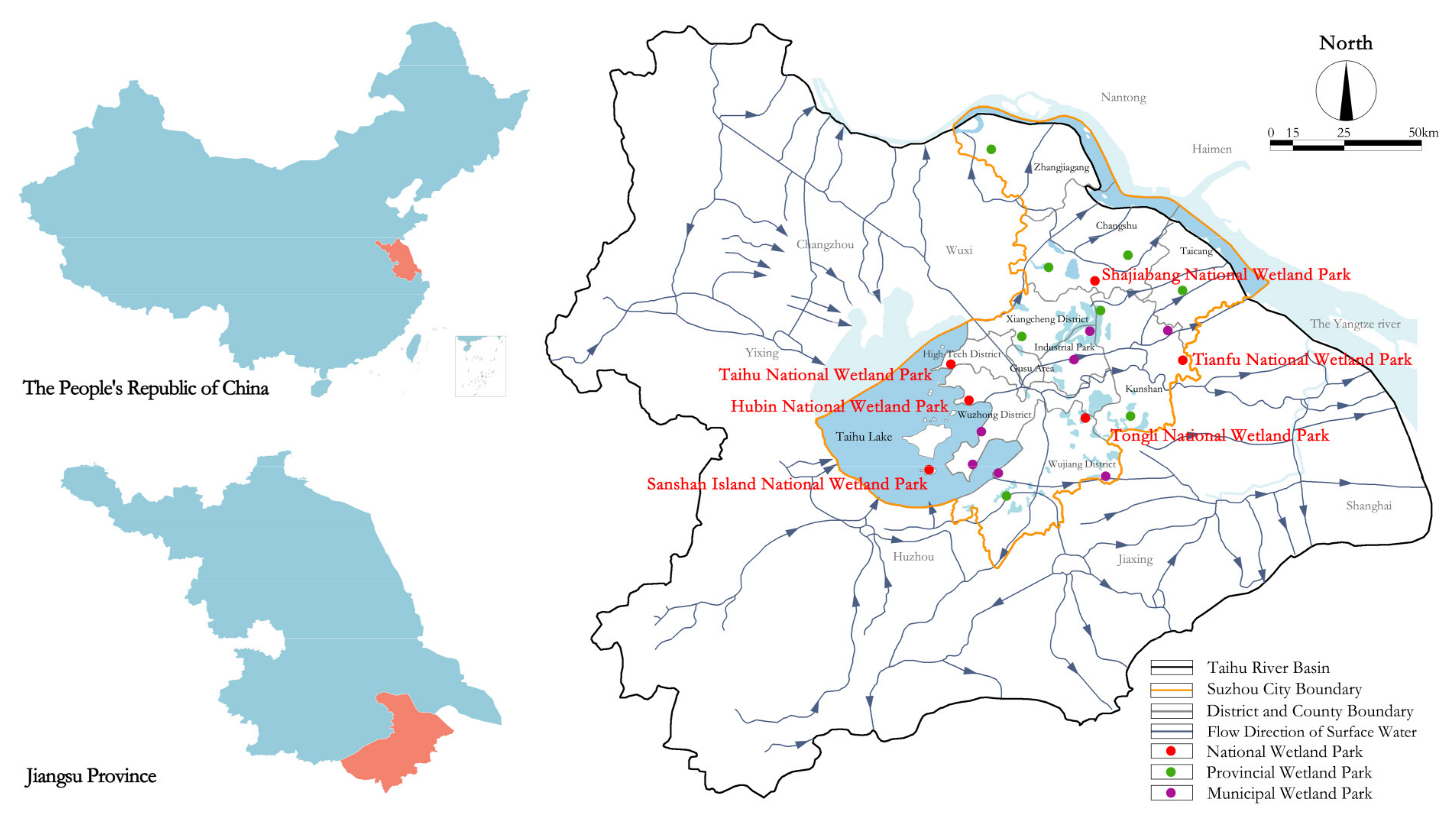
Suzhou (30°45′–32°2′ N, 119°55′–121°22′ E) is located in the southeast region of Jiangsu Province (30°45′−35°7′ N, 116°21′−121°56′), Eastern China. The region has a subtropical monsoon climate with an average annual temperature of 15.7 °C and average annual precipitation of 1100 mm yr⁻¹. Taihu Lake is the third-largest freshwater lake in China and an important water source for the Suzhou National Wetland Park. Suzhou now has 21 national, provincial, and municipal wetland parks, and 102 municipal-level important wetlands (Figure 1). Suzhou National Wetland Park can be divided into four types of landscape structures: block-like uniform, multi-layer cofferdam, multi-pond structure, and block-shaped agglomeration (

Table 1. The four types of wetland landscape structure.

Type	a. Block-Like Uniform	b. Multi-Layer Cofferdam	c. Multi-Pond Structure	d. Block-Shaped Agglomeration
Graphic
Interpretation	Patch size and distance between land and water patches are relatively uniform. Dams are situated within the water surface with deep and open water. The wetland is formed by many small ponds connected by water ditches. Water and land are clustered to form plaques.

Water, Land.

). Each year can be divided into four periods, consisting of a dry season (December–February), two normal seasons (March–May, September–November), and a rainy season (June–August).

2.2. Data Collection

2.2.1. Landscape Data

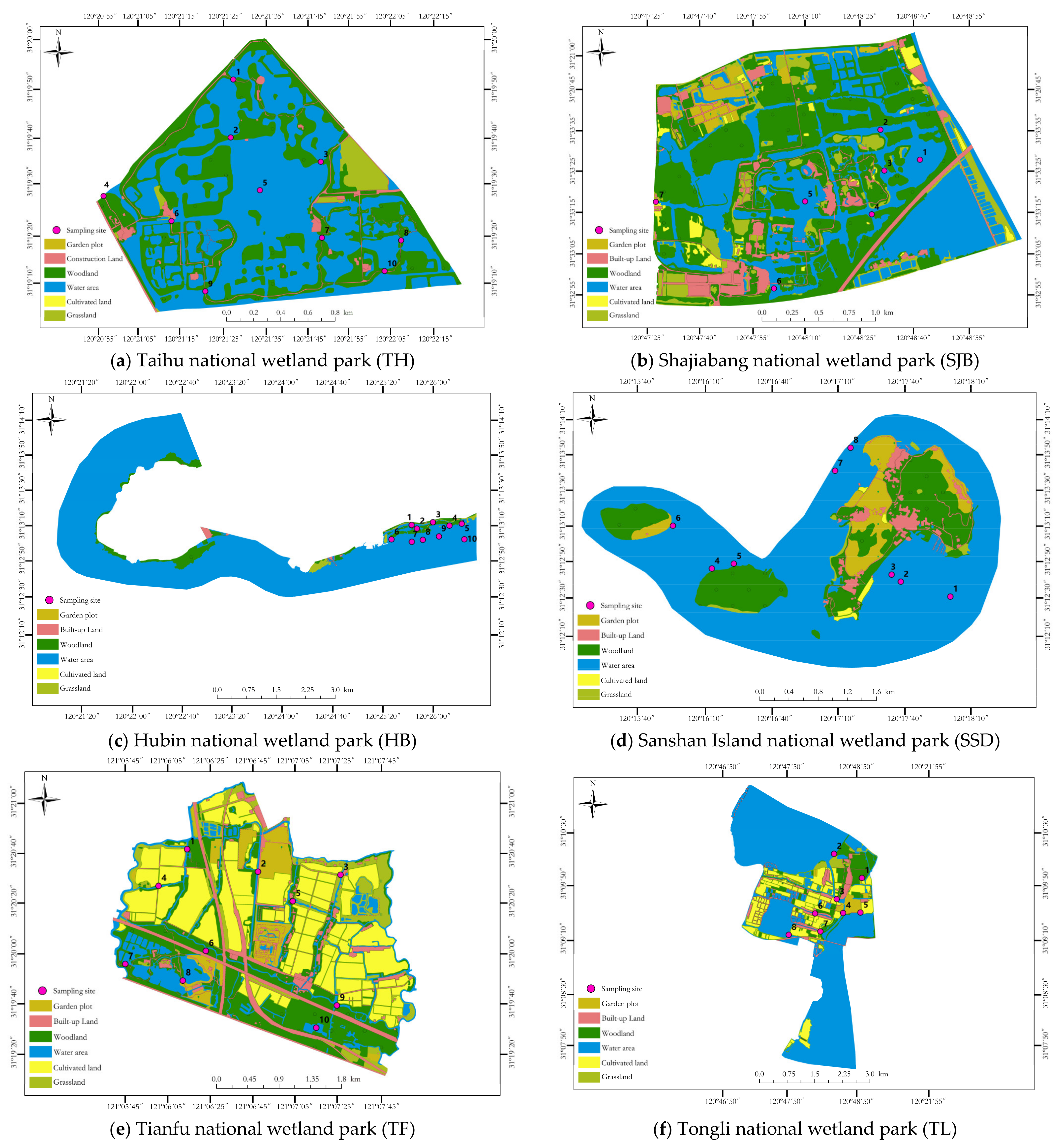
Image data were sourced from the Gaofen-2 satellite (China Aerospace Science and Technology Corporation, Beijing, China), the ground information was collected using ArcGIS10.6 (Environmental Systems Research Institute, Inc., RedLands, CA, USA), and the vector data of wetland park landscape type maps were obtained by visual interpretation. Based on the current land use classification (GB/T21010–2017), this paper divides the land cover of wetland parks into water area, woodland, garden plot, grassland, cultivated land, and built-up land (Figure 2). Water quality was sampled at 53 sites that were selected according to different functional zoning (

Table 2. Distribution of sampling points in Suzhou National Wetland Park.

Wetland Park	Landscape Structure	Functional Zoning
		Conservation	Restoration and Reconstruction	Rational Utilization
Taihu	Block-like uniform	8, 9, 10	1, 2, 3, 5	4, 6, 7
Shajiabang		1, 2, 3	4, 6	5, 7
Hubin	Multi-layer cofferdam	7, 8, 9, 10		1, 2, 3,4, 5, 6
Sanshan Island		4, 5, 6, 7, 8	1	2,3
Tianfu	Multi-pond structure	1, 2, 4, 6, 10	3, 5	7, 8, 9
Tongli	Block-shaped agglomeration	2, 5, 8	3,4	1, 6, 7

; for names of the parks see Figure 2).

2.2.2. Water Quality Data

Total nitrogen, total phosphorous, dissolved oxygen, chemical oxygen demand, and biological oxygen demand were measured from water samples collected from each study site. Samples were collected monthly from February 2019 to January 2020 at times when the weather was sunny with low wind speed and no recent heavy rain. A plexiglass water sampler was placed vertically in the water, and samples were collected from 0.5 m and 1 m below the water surface and transferred into bottles. The sampling depth was calculated by combining the water depth of each sampling point. Dissolved oxygen was measured in the field. All other samples were transported to the Tianfu National Wetland Park laboratory, and water quality variables were measured using methods outlined in

Table 3. Water quality parameters and experimental methods.

Parameter		Unit	Measurement Methods	Instrument Model and Manufacturer
TN	Total Nitrogen	mg/L	Ultraviolet and visible spectrophotometry	759S, Lingguang Technology Co., Ltd., Shanghai, China
TP	Total Phosphorous	mg/L	Ammonium molybdate spectrophotometry	JH-TD02, Jinghong Environmental Protection Technology Co., Ltd., Qingdao, China
DO	Dissolved Oxygen	mg/L	Portable dissolved oxygen analyzer	JPB-607A, Yifen Scientific Instrument Co., Ltd., Shanghai, China
COD	Chemical Oxygen Demand	mg/L	Potassium dichromate method	STAEHD-106B, Shengtai Electronic Technology Co., Ltd., Jinan, China
BOD	Biological Oxygen Demand	mg/L	Incubator dilution and inoculation	HWS-150B, Deshi Technology Co., Ltd., Beijing, China

. All variables were measured in triplicate and an average determined for use in the analysis.

2.3. Indices Analysis

2.3.1. Landscape Pattern

FRAGSTATS4.2 (Oregon State University, Corvallis, OR, USA) developed by Dr. McGarigal was used to calculate landscape indices [45]. Eight commonly used indices were selected from patch level, class level, and landscape level to represent landscape fragmentation, aggregation, dominance, and diversity. At the patch level, we used the index PLAND. At the class level, there were six indices, including NP, PD, LPI, LSI, and AI. At the landscape level, there were three indices, including CONTAG, SHDI, and COHES (for abbreviations and equations, see

Table 4. Landscape index selection.

Landscape Index		Unit	Calculation	Significance
NP	Number of Patches	PCS	$\mathrm{NP}=\mathrm{n}$i	Landscape fragmentation
PD	Patches Density	PCS/100ha	$\mathrm{PD}=\frac{{\mathrm{n}}_{\mathrm{i}}}{\mathrm{A}}\times {10}^6$
LSI	Landscape Shape i	None	$\mathrm{LSI}=\frac{0.25\mathrm{E}}{\sqrt{\mathrm{A}}}$
CONTAG	Contagion	%	$\mathrm{CONTAG}=\left[1+\frac{{{\displaystyle \sum }}_{\mathrm{i}=1}^{\mathrm{m}}{{\displaystyle \sum }}_{\mathrm{j}=1}^{\mathrm{n}}[({\mathrm{P}}_{\mathrm{i}})({\mathrm{g}}_{\mathrm{ik}})][\ln {\mathrm{p}}_{\mathrm{i}}({\mathrm{g}}_{\mathrm{ik}}{{\displaystyle \sum }}_{\mathrm{k}=1}^{\mathrm{m}}{\mathrm{g}}_{\mathrm{ik}})]}{2\ln \mathrm{m}}\right]\times 100$	Landscape aggregation
AI	Aggregation index	%	$\mathrm{AI}=[1+{{\displaystyle \sum }}_{\mathrm{i}=1}^{\mathrm{m}}{{\displaystyle \sum }}_{\mathrm{j}=1}^{\mathrm{n}}\frac{{\mathrm{P}}_{\mathrm{ij}}\ln {\mathrm{P}}_{\mathrm{ij}}}{2\ln \mathrm{m}}]\times 100$
COHES	Patch Cohesion index	None	$\mathrm{COHES}=\left[1-\frac{{{\displaystyle \sum }}_{\mathrm{i}=1}^{\mathrm{m}}{\mathrm{P}}_{\mathrm{ij}}}{{{\displaystyle \sum }}_{\mathrm{j}=1}^{\mathrm{m}}{\mathrm{P}}_{\mathrm{ij}}\sqrt{{\mathrm{a}}_{\mathrm{ij}}}}\right]{\left[1-\frac{1}{\sqrt{\mathrm{A}}}\right]}^{-1}\times 100$
LPI	Largest Patch index	%	$\mathrm{LPI}=\frac{\max ({\mathrm{a}}_1,\dots ,{\mathrm{a}}_{\mathrm{n}})}{\mathrm{A}}\times 100$	Landscape dominance
PLAND	Percentage of landscape	%	$\mathrm{PLAND}={\mathrm{P}}_{\mathrm{i}}=\frac{{{\displaystyle \sum }}_{\mathrm{j}=1}^{\mathrm{n}}{\mathrm{a}}_{\mathrm{ij}}}{\mathrm{A}}\times 100$
SHDI	Shannon’s Diversity Index	None	$\mathrm{SHDI}=-{{\displaystyle \sum }}_{\mathrm{i}=1}^{\mathrm{m}}({\mathrm{P}}_{\mathrm{i}}\ln {\mathrm{P}}_{\mathrm{i}})$	Landscape diversity

n_i is the total area of landscape parameter i, A is the total area of all landscape parameters, E is the total length of all patch boundaries, P_i is the proportion of a specific patch type i within a landscape, g_ik is the number of adjacent patches of type i and type k, m is the total number of patch types in the landscape, P_ij is the perimeter of the j-th patch in type i landscape, a_ij is the area of the j-th patch in type i landscape.

).

2.3.2. Water Quality

(1)

Single factor identification index

The single factor water quality index (F_i) of the ith water quality parameter consisted of a one-digit integer with two or three significant figures after the decimal point [46]:

F_i = X₁X₂X₃

(1)

The value of X₁ is the water quality class of the ith water quality parameter. The value of X₂ is the position of the ith water quality parameter within the range of the X₁ water quality class, which is calculated and determined according to the rounding principle. The value of X₃ is the result of the comparison between the measured class of water quality parameter with the target class.

If the class of water quality parameters was better than the limits value of class V, the values of X₁ were determined according to

Table 5. Class limits for different water quality parameters (unit: mg/L).

Parameter		Class I	Class II	Class III	Class IV	Class V	Inferior to Class V
If	TN	0.2≤	0.5≤	1.0≤	1.5≤	2.0≤	>2.0
	TP	Moving: 0.02≤ Still: 0.01≤	Moving: 0.1≤ Still: 0.025≤	Moving: 0.2≤ Still: 0.05≤	Moving: 0.3≤ Still: 0.1≤	Moving: 0.4≤ Still: 0.2≤	Moving: >0.4 Still: >0.2
	COD	15≤	15≤	20≤	30≤	40≤	>40
	BOD	3≤	3≤	4≤	6≤	10	>10
	DO	Saturation rate of 90% or ≥7.5	≥6	≥5	≥3	≥2	<2
Then	X1	1	2	3	4	5	6

Values denote the lower limit for DO and the upper limit for all other parameters.

. The larger the value of DO, the better the water quality. The larger the value of TN, TP, COD, and BOD, the worse the water quality. Therefore, the calculation of the value of X₂ was divided into DO and non-DO parameters. The calculation formulas are shown in (2) and (3).

$$\mathrm{DO}: { \mathrm{X}}_2=\frac{{\mathsf{\rho }}_{\mathrm{DO},\mathrm{upper} \mathrm{limit}}-{\mathsf{\rho }}_{\mathrm{DO},\mathrm{measured} \mathrm{value}}}{{\mathsf{\rho }}_{\mathrm{DO},\mathrm{higher} \mathrm{limit}}-{\mathsf{\rho }}_{\mathrm{DO},\mathrm{lower} \mathrm{limit}}}\times 10, {\mathrm{X}}_1\in (1,2,3,4,5)$$

(2)

$$\mathrm{Non}-\mathrm{DO}: {\mathrm{X}}_2=\frac{{\mathsf{\rho }}_{\mathrm{i},\mathrm{measured} \mathrm{value}}-{\mathsf{\rho }}_{\mathrm{i},\mathrm{lower} \mathrm{limit}} }{{\mathsf{\rho }}_{\mathrm{i},\mathrm{upperr} \mathrm{limit}}-{\mathsf{\rho }}_{\mathrm{i},\mathrm{lower} \mathrm{limit}}}\times 10, {\mathrm{X}}_1\in (1,2,3,4,5)$$

(3)

If the class of water quality parameters was inferior to or equal to the limit value of class V, the values of X₁.X₂ were calculated as a whole. The calculation of the value of X₁.X₂ was divided into DO and non-DO parameters. When the water quality was very poor, DO may not have been measured. If the correction coefficient m was not introduced, X₁.X₂ = 6 would occur; that is, DO was equal to the lower limit of class V, which was inconsistent with reality. The calculation formulas are shown in (4) and (5).

$$\mathrm{DO}: {\mathrm{X}}_1{\mathrm{X}}_2=6+\frac{{\mathsf{\rho }}_{\mathrm{DO},\mathrm{lower} \mathrm{limit}}-{\mathsf{\rho }}_{\mathrm{DO}}}{{\mathsf{\rho }}_{\mathrm{DO},\mathrm{lower} \mathrm{limit}}}\times \mathrm{m}$$

(4)

$$\mathrm{Non}-\mathrm{DO}: {\mathrm{X}}_1{\mathrm{X}}_2=6+\frac{{\mathsf{\rho }}_{\mathrm{i}}-{\mathsf{\rho }}_{\mathrm{i},\mathrm{upperr} \mathrm{limit}}}{{\mathsf{\rho }}_{\mathrm{i},\mathrm{upperr} \mathrm{limit}}}$$

(5)

X₃ was the second digit after the decimal point, and its value was determined by comparing the measured class and target class of water quality parameters. If the class of the measured value was better than or reached the class of the target value, X₁ ≥ f_i, then X₃ = 0. If the class of the measured value was worse than the class of target value, X₁ < f_i. The calculation formulas are shown in (6) and (7); f_i is the target class of water quality.

X₃ = X₁ − f_i (X₂ ≠ 0)

(6)

X₃ = X₁ − f_i − 1 (X₂ = 0)

(7)

(2)

Comprehensive identification index

The comprehensive identification index (I_wq) consisted of X₁, X₂, X₃, and X₄. Where X₁.X₂ was the average value of the sum of the single factor identification indices, X₃ was the number of water quality parameters inferior to the class limits of the target value. X₄ was the result of the comparison between the measured class and the target class, and it was determined by the number of non-zero X₃ in the single factor identification index (PI) [47]. The formula is as follows:

I_wq = X₁X₂X₃X₄

(8)

X₁.X₂ consisted of a one-digit integer and the first digit after the decimal point, and X₁.X₂ = ∑(P_1′ + P_2′ + ∧ + P_m’)/m. m were the numbers of water quality parameters. P₁’, P₂’…P_m’ are the single factor water quality indices of 1st, 2nd,…, mth water quality values. The judgment criteria for the comprehensive water quality classes are shown in

Table 6. Determination of water quality class by comprehensive water quality identification index method.

Judgment Criteria	Class of Measured Value
1.0 ≤ X1.X2 ≤ 2.0	Class I
2.0 < X1.X2 ≤ 3.0	Class II
3.0 < X1.X2 ≤ 4.0	Class III
4.0 < X1.X2 ≤ 5.0	Class IV
5.0 < X1.X2 ≤ 6.0	Class V
6.0 < X1.X2 ≤ 7.0	Inferior to class V but not black smelly
X1.X2 > 7.0	Inferior to class V and black smelly

.

2.3.3. Correlation Analysis

Pearson’s correlation analysis of landscape indices and water quality parameters was performed using SPSS23.0 (IBM, Armonk, NY, USA). A one-sided test was used to test the significance between the landscape indices and the water quality parameters, and the index with a significant correlation coefficient (P < 0.05) was selected for further analysis [48].

Multiple stepwise regression analyses were then used to explore the response relationship between landscape indices and water quality parameters.

$$\mathrm{y}={\mathrm{b}}_0+{\mathrm{b}}_1{\mathrm{x}}_1+{\mathrm{b}}_2{\mathrm{x}}_2+\dots +{\mathrm{b}}_{\mathrm{k}}{\mathrm{x}}_{\mathrm{k}}$$

(9)

In the formula, y was the dependent variable and represented the value of the water quality parameters. x₁, x₂,..., x_k as independent variables represented the landscape indices. b₁, b₂,..., b_k were influence coefficients and b₀ represented a constant.

The comprehensive relationship between landscape indices and water quality parameters was determined by redundancy analysis. In the sequence diagram, the length of the landscape index arrow reflected the impact of landscape indices on water quality parameters. The longer the arrow length, the greater the influence.

3. Results and Analysis

3.1. Landscape Structure Characteristics of Suzhou National Wetland Park

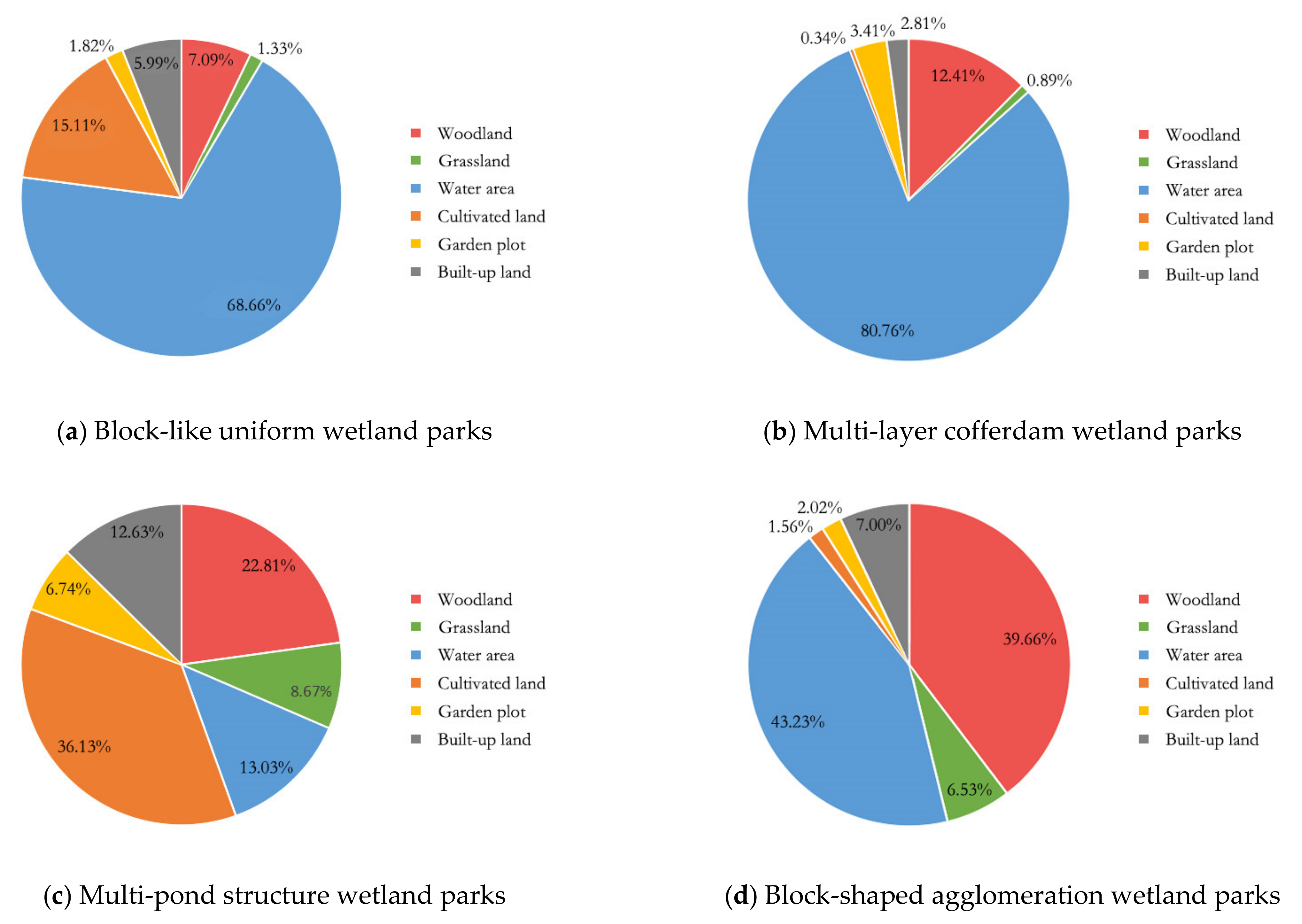
Taihu (TH) and Shajiabang (SJB) were block-like uniform type wetland parks, and the landscape patches were distributed in a balanced manner, with woodland accounting for 35–40% of the area. Hubin (HB) and Sanshandao (SSD) were multi-layer cofferdam type wetland parks, and the landscape patches were distributed in circular and zonal patterns, with the maximum proportion of water accounting for 70% to 90%. Tianfu (TF) was a multi-pond structure type wetland park, and the landscape patches were distributed in the shape of tweezers. Cultivated land and woodland were the main areas, each accounting for 20–35% of the space. Tongli (TL) was a block-shaped agglomeration wetland park, and the landscape patches were distributed in clusters, with the maximum proportion of water accounting for 50–70% (Figure 3).

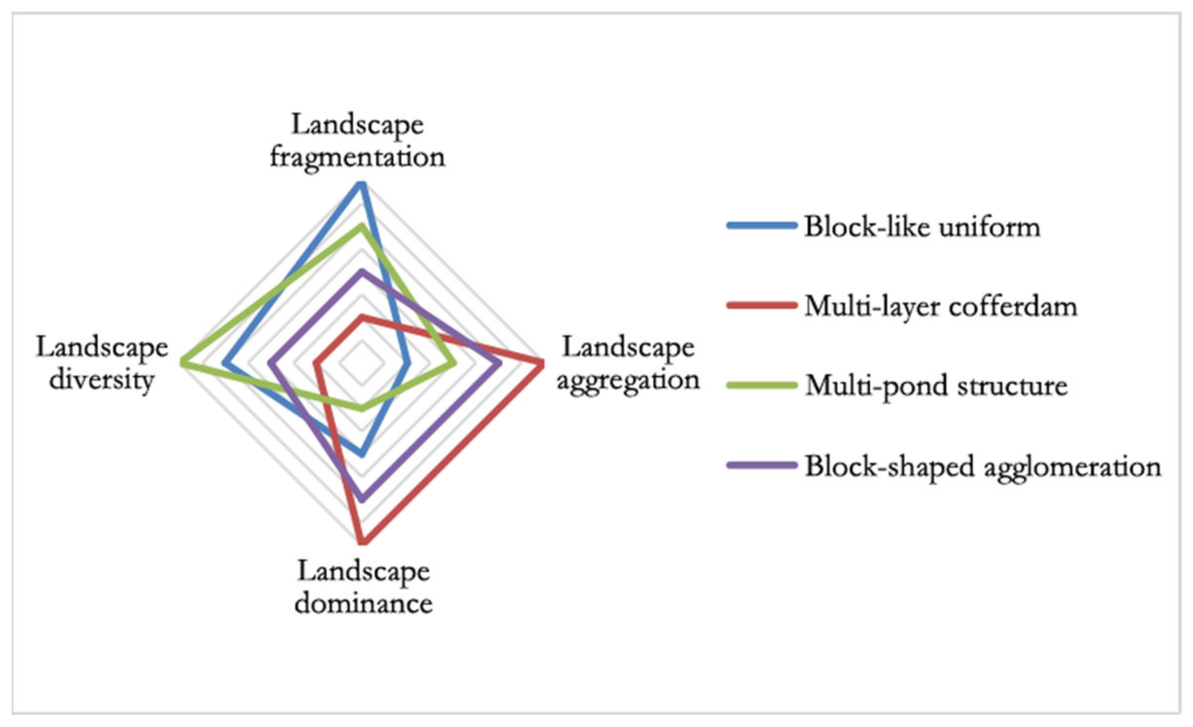
The block-like uniform wetland parks had the highest fragmentation, the lowest aggregation, a low degree of dominance, and high diversity. Multi-layer cofferdam wetland parks had the lowest fragmentation, the highest aggregation, the highest dominance, and the lowest diversity. Multi-pond structure wetland parks had a high degree of fragmentation, low aggregation, the lowest dominance, and the highest diversity. Block-shaped agglomeration wetland parks had low fragmentation, high aggregation, high dominance, and low diversity (

Table 7. Mean value of landscape index of Suzhou National Wetland Park with different landscape structures.

Landscape Structure	Parks	Fragmentation				Aggregation				Dominance		Diversity
		NP	PD	LSI	Value	CONTAG	AI	COHES	Value	LPI	Index	SHDI	Value
Block-like uniform	TH	432	0.87	21.60	Highest	61.55	98.56	99.63	Lowest	19.68	Low	1.37	High
	SJB
Multi-layer cofferdam	HB	67	0.05	6.41	Lowest	81.02	99.25	99.96	Highest	81.01	Highest	0.62	Lowest
	SSD
Multi-pond structure	TF	476	0.43	26.28	High	52.02	98.54	99.80	Low	11.07	Lowest	1.63	Highest
Block-shaped agglomeration	TL	238	0.15	12.46	Low	70.22	99.47	99.86	High	69.04	High	0.94	Low

).

The difference in landscape pattern index between block-like uniform and multi-layer cofferdam wetlands was the largest. The difference in landscape pattern index between block-like uniform and multi-pond structure wetlands was the smallest. The indices for block-shaped agglomeration wetlands were more balanced (Figure 4).

3.2. Water Quality Characteristics of Suzhou National Wetland Park

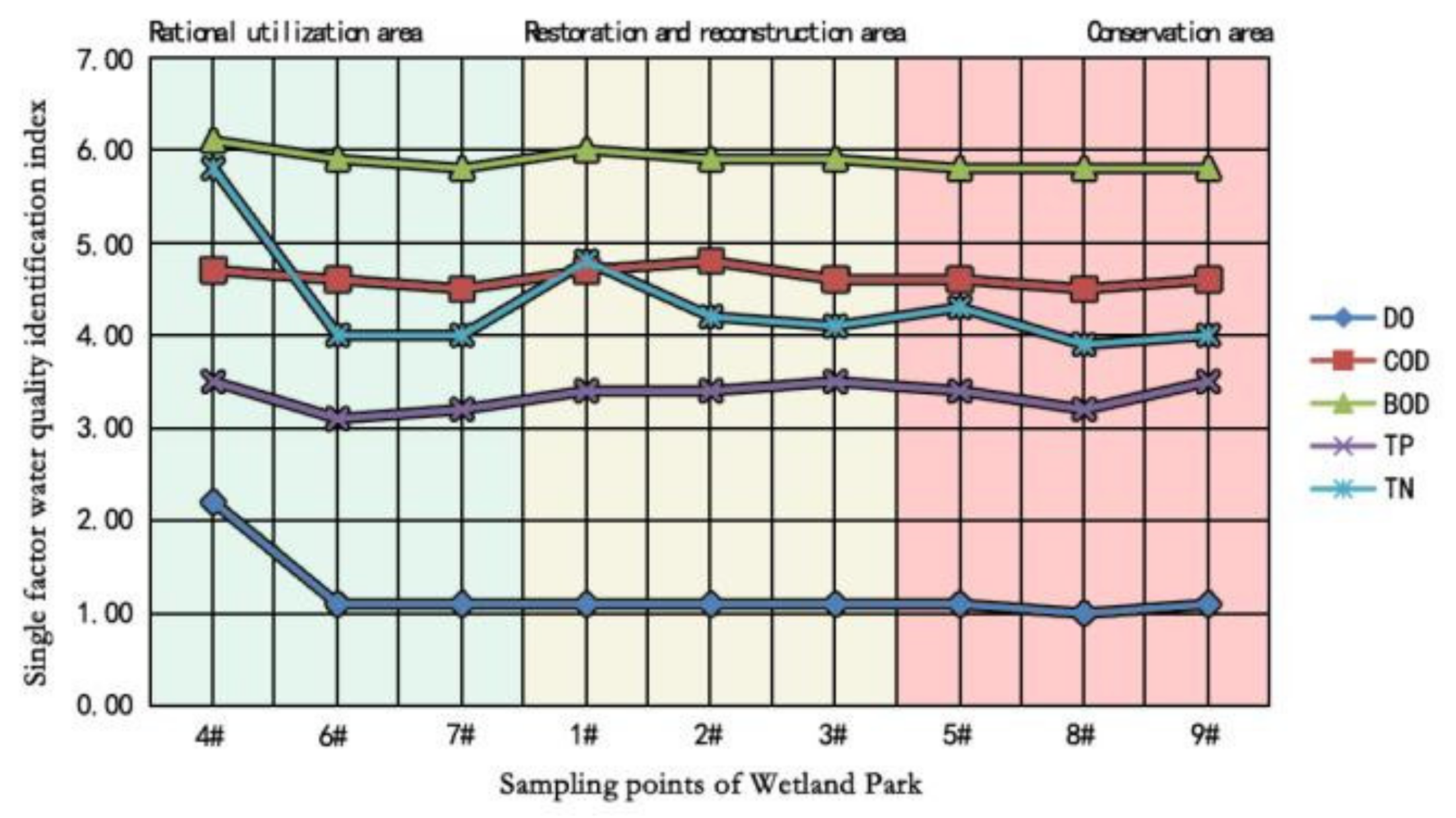
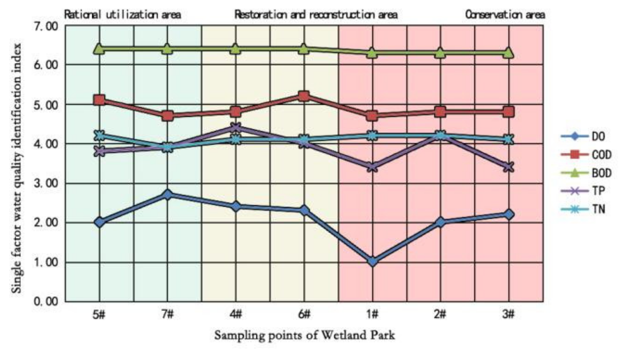
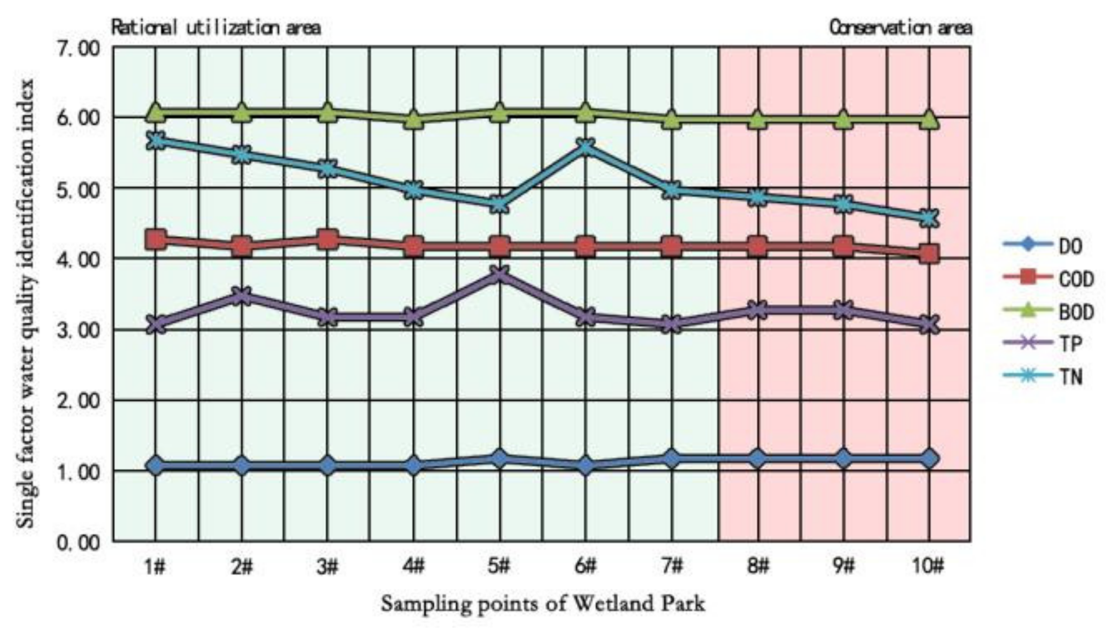
The single factor identification index method was used to arrange the pollution degree of TH water quality parameters from highest to lowest and revealed that BOD > COD > TN > TP > DO. Sampling sites number 1, 2, and 4, located in the north of the wetland park, upstream of the water system, and close to the urban residential area, had the highest parameter values under the influence of human factors. Sampling sites 8 and 10 were located downstream of the river system and had the lowest parameter values. The ranking of SJB water quality parameter values from highest to lowest was BOD > COD > TN > TP > DO. Sampling site number 6, nearest to the entrance, and number 5, in the central tourist area, were most affected by human interference. Sampling site number 4 was originally a mulberry fishpond, and although it has been abandoned for many years, the TP was still high. The ranking of HB water quality parameter values from highest to lowest was BOD > TN > COD > TP > DO. Sites 7, 8, 9, and 10, which were farthest from the shore, had the best water quality parameter values. Sites 1, 3, and 5, which were closest to the shore, had the worst water quality parameter values due to the human disturbances that occur urban residential areas.

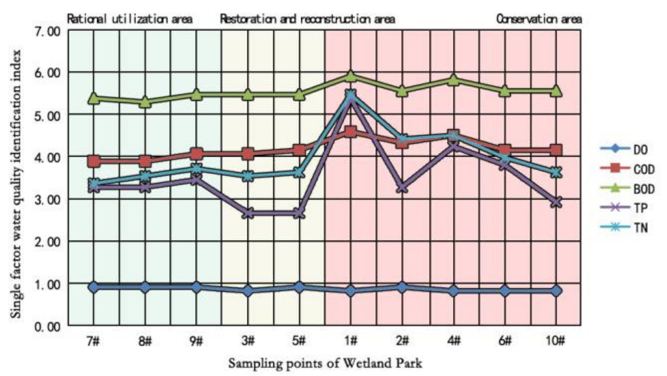
The ranking of SSD water quality parameter values from highest to lowest was BOD > TN > TP > COD > DO. Large scale ecological floating islands in sampling sites 1, 2, and 3 had a remarkable effect on water purification, while the water flow velocity of sampling sites 4, 5, and 6 was fast and the water quality was poor. The ranking of TF water quality parameter values from highest to lowest was BOD > COD > TN > TP > DO. Sites 1 and 4 were close to urban built-up areas and located downstream of the water system with poor water quality. Sites 7, 8, and 10 were separated from the main body of the wetland park by the East–West railway, were less affected by external interference, and had better water quality. The ranking of TL water quality parameter values from highest to lowest was BOD > TN > COD > TP > DO. The water quality of the sampling sites in the east and downstream of the wetland park was better than the upstream sampling sites because TL was the more recently built, the total capital investment was the least, and the external water system has a considerable impact on the water quality (Figure 5, Figure 6, Figure 7, Figure 8, Figure 9 and Figure 10).

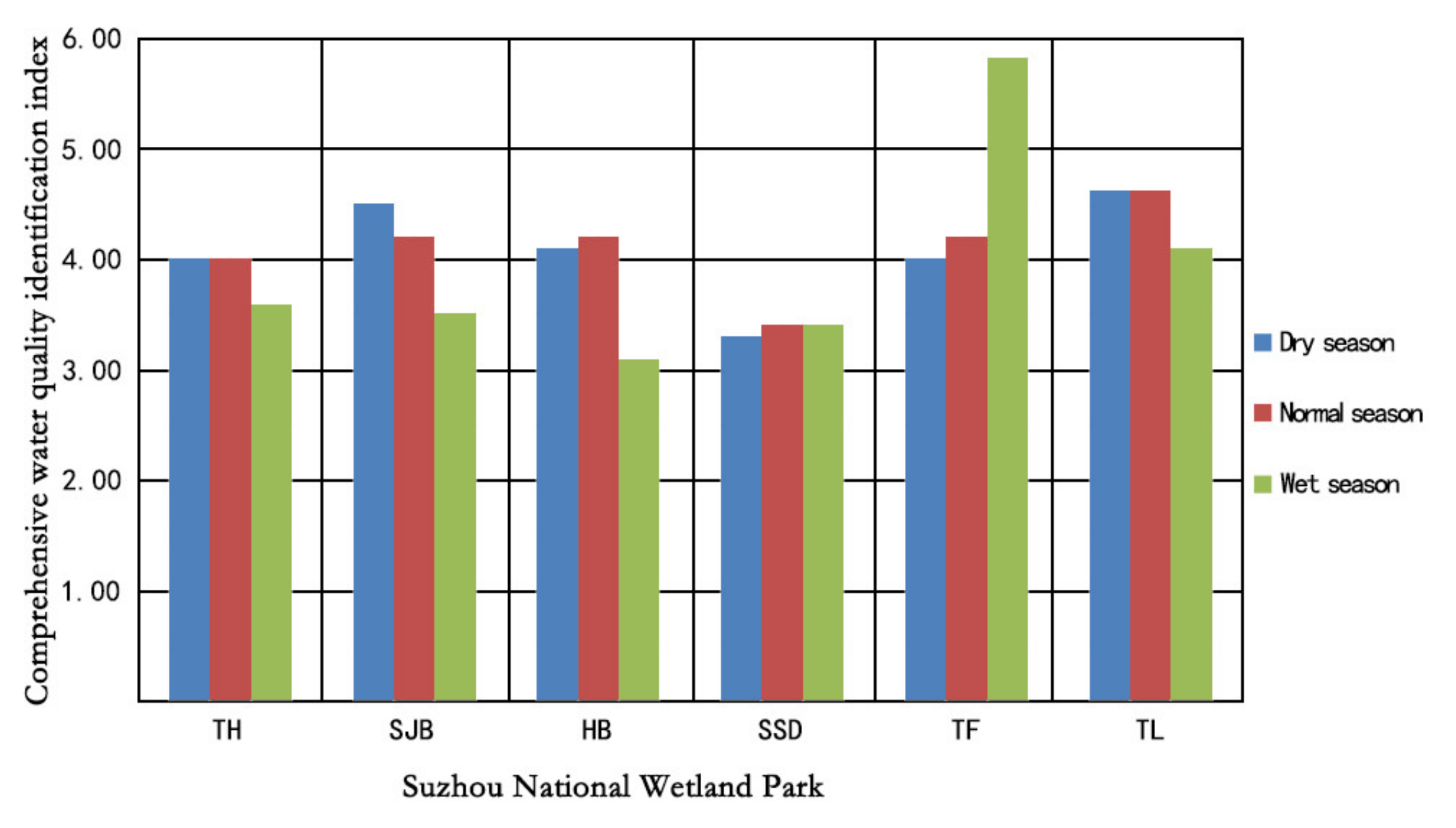
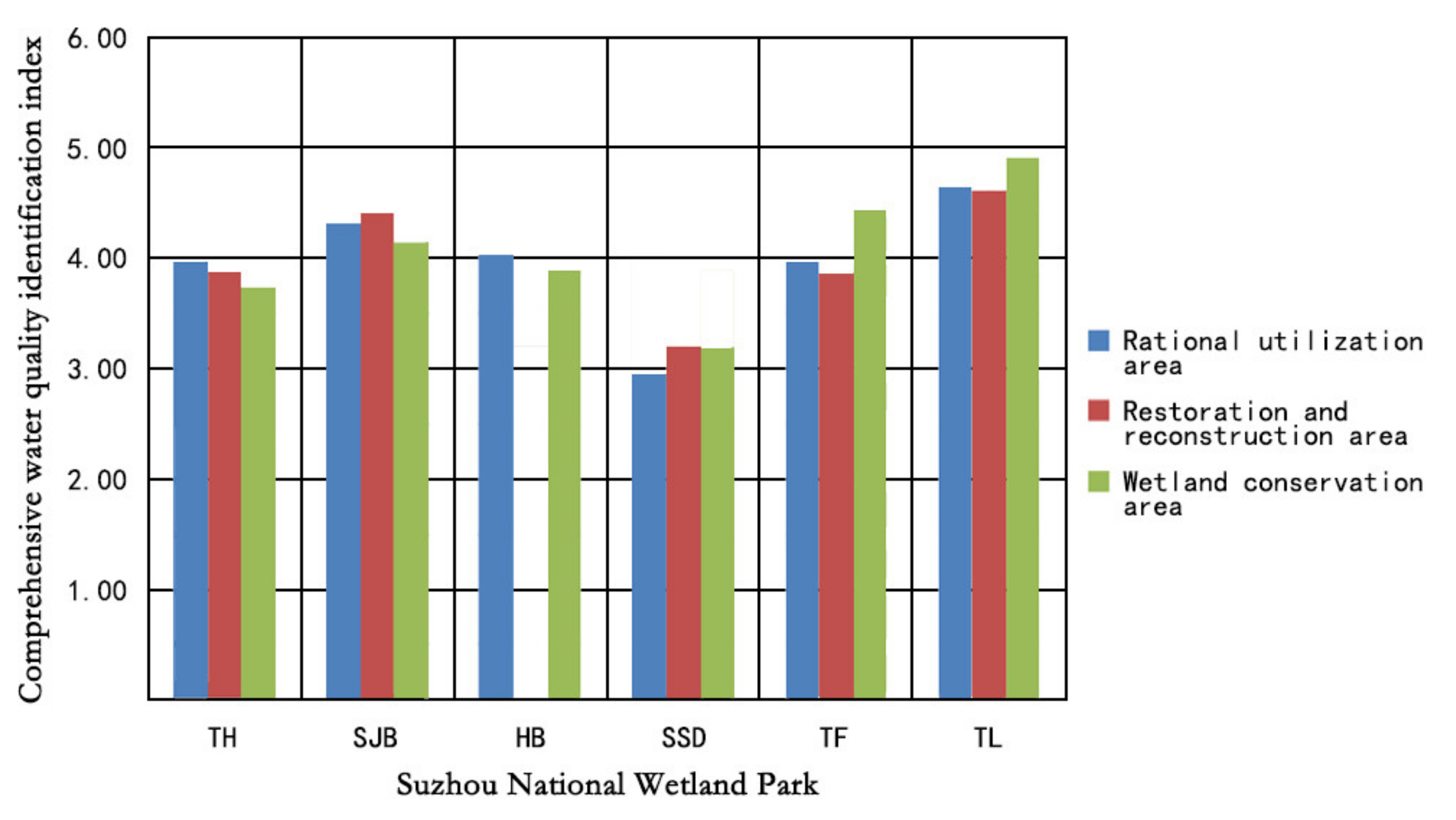
The water quality of wetland parks ranked from good to bad was SSD > TH, SJB, HB > TL, TF. The results show that SSD water quality was class III for the whole year, while TH, SJB, and HB water quality was class IV in the dry and normal seasons and improved to class III in the rainy season. The water quality at TL also improved during the rainy season but remained in class IV throughout the year. TF water quality was class IV in the dry season and normal season, but it decreased to class V during the rainy season (Figure 11). Comparative analysis of water quality in different functional zones revealed that the pollution at TH, SJB, HB, and TL was greatest in the rational utilization area, followed by the restoration and reconstruction area, and lowest in the conservation area. Changes in the comprehensive identification index ranged from class III to class IV. The pollution at SSD was greatest at the restoration and reconstruction area, then at the conservation area, and at the rational utilization area. The rational utilization area was class II, which was the best among all wetland parks. The worst water quality in TF wetland conservation area was class IV, and water quality in rational utilization area was better than in the restoration and reconstruction areas, both of which were class III (Figure 12).

3.3. Correlation between Landscape Structure and Water Quality

3.3.1. Correlation between Landscape Types and Water Quality

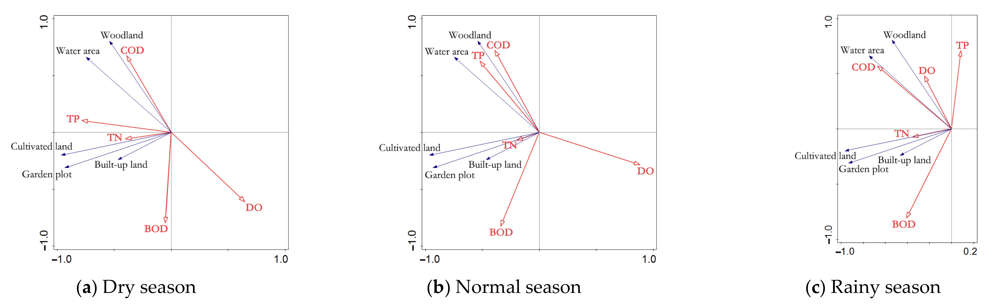
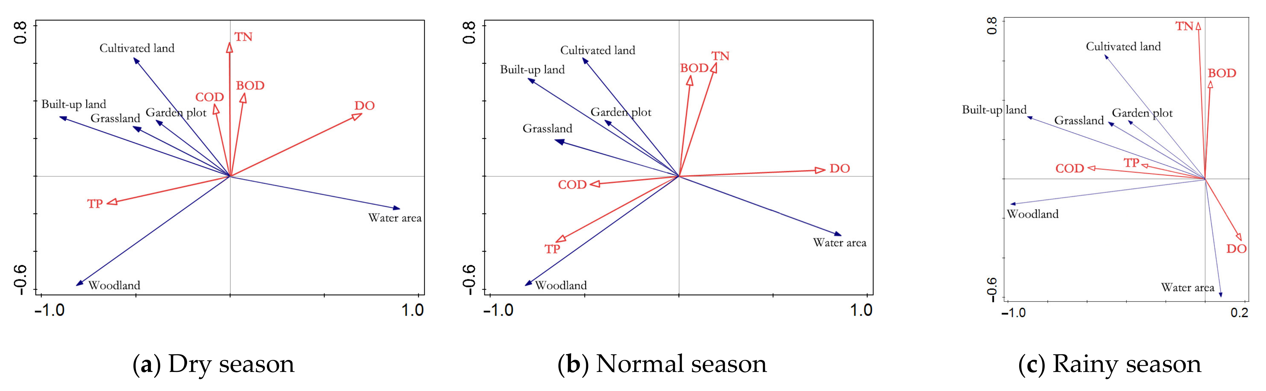
The areas of different landscape types in the Suzhou National Wetland Park were compared with water quality parameters in different seasons. The PLAND of cultivated land did not conform to the normal distribution (P > 0.05). The order of water purification effects of landscape types from best to worst was water area and woodland > garden plot and grassland > built-up land. The larger the PLAND of the water area, the better the water quality, especially for TP, DO, and COD. The effect of the PLAND on water purification for the garden plot and woodland was not clear. For example, the garden plot had a positive ecological effect on TN and COD but a negative one on DO and BOD. Woodland had a positive ecological effect on TN but a negative one on TP and DO. The larger the PLAND of grassland and built-up land, the worse the improvement in water quality. For example, grassland had a negative ecological effect on TP and DO but had no clear correlation with other indices, and built-up land had negative ecological effects on TN, TP, DO, COD, and BOD.

The impact of patch area on the water quality index in the rainy season appeared to be the most important factor, with both positive ecological effects of water area and woodland patches, and the negative effects of the garden plot and built-up land patches being significant. The impact of patch area on the water quality index in the normal season was the second most important factor, with the positive ecological effects of water area and garden plot patches and the negative ecological effects of grassland and built-up land being significant (

Table 8. Multiple regression analysis between proportion of landscape area and water quality index.

Period	Index	Multivariate Regression Model	R2	Adjusted R2	P
Dry season	DO	10.505 − 0.284 grassland	0.801	0.735	0.040
Normal season	TP	0.123 + 0.010 grassland	0.689	0.611	0.041
	DO	9.404 − 0.322 built-up land	0.920	0.893	0.010
Rainy season	BOD	7.430 + 1.175 garden plot	0.965	0.956	0.000

, Figure 13).

3.3.2. Correlation between Spatial Configuration and Water Quality

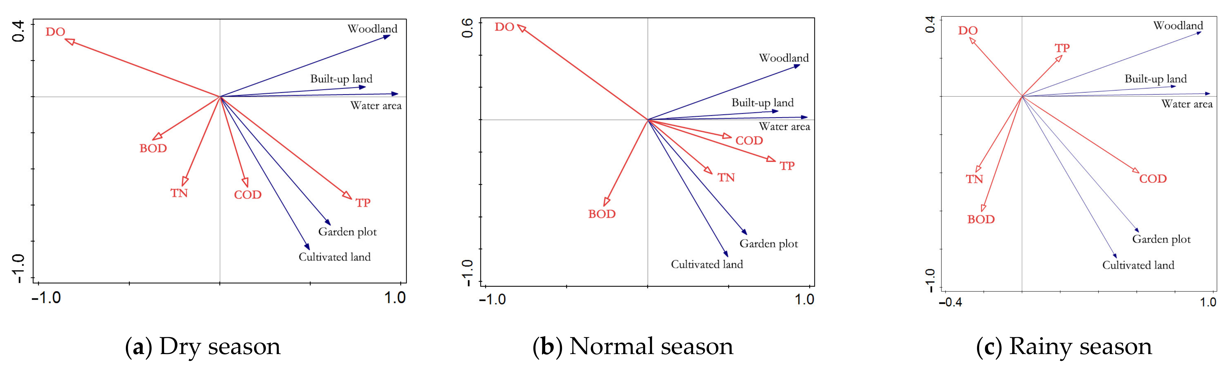
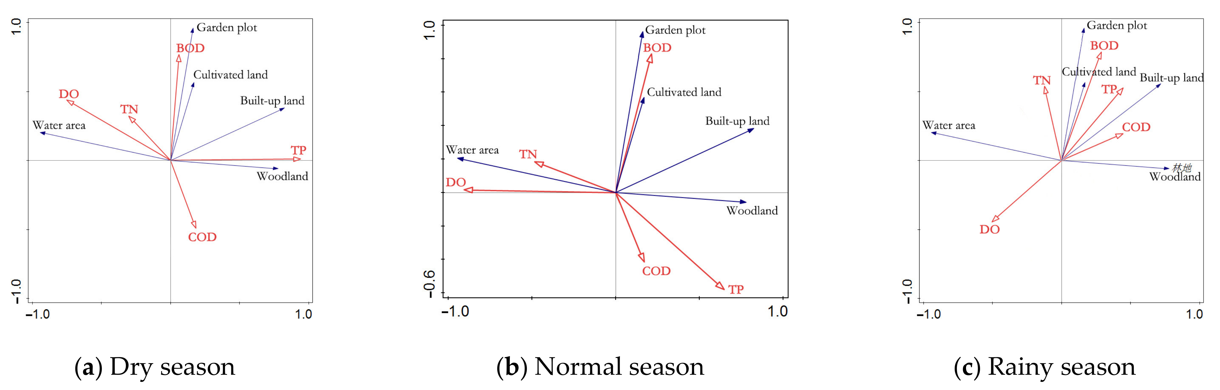
The NP of the grassland did not conform to the normal distribution (P > 0.05). The results show that the water area had a positive significant correlation with TP and COD and a highly significant negative correlation with DO. Woodland had a positive significant correlation with TP and COD and a negative significant correlation with DO. The garden plot had a positive significant correlation with TN, TP, COD, and BOD and a negative significant correlation with DO. Cultivated and built-up land both had positive significant correlations with TN, TP, and COD. Built-up land also had a negative significant correlation with DO.

The number of garden plot and cultivated land patches had a greater impact on water quality parameters in the rainy season, where a higher number of patches resulted in worse water quality. The effect of season on the relationships between water area, woodland, built-up land, and water quality remains unclear. In conclusion, the higher the NP, the worse the water quality and the higher the degree of fragmentation of the landscape, which is not conducive to the interception and prevention of pollutants entering the waterways (

Table 9. Multiple regression analysis between patch number and water quality.

Period	Index	Multivariate Regression Model	R2	Adjusted R2	P
Dry season	TP	0.112 + 0.001 built-up land	0.753	0.692	0.025
	DO	10.608 − 0.018 water area	0.908	0.878	0.012
Normal season	TP	0.116 + 0.001 water area	0.796	0.746	0.017
	DO	8.901 − 0.018 water area	0.955	0.940	0.040
Rainy season	TN	1.141 + 0.018 cultivated land − 0.005 water area	0.964	0.940	0.007
	COD	11.338 + 0.148 water area	0.682	0.602	0.043

, Figure 14).

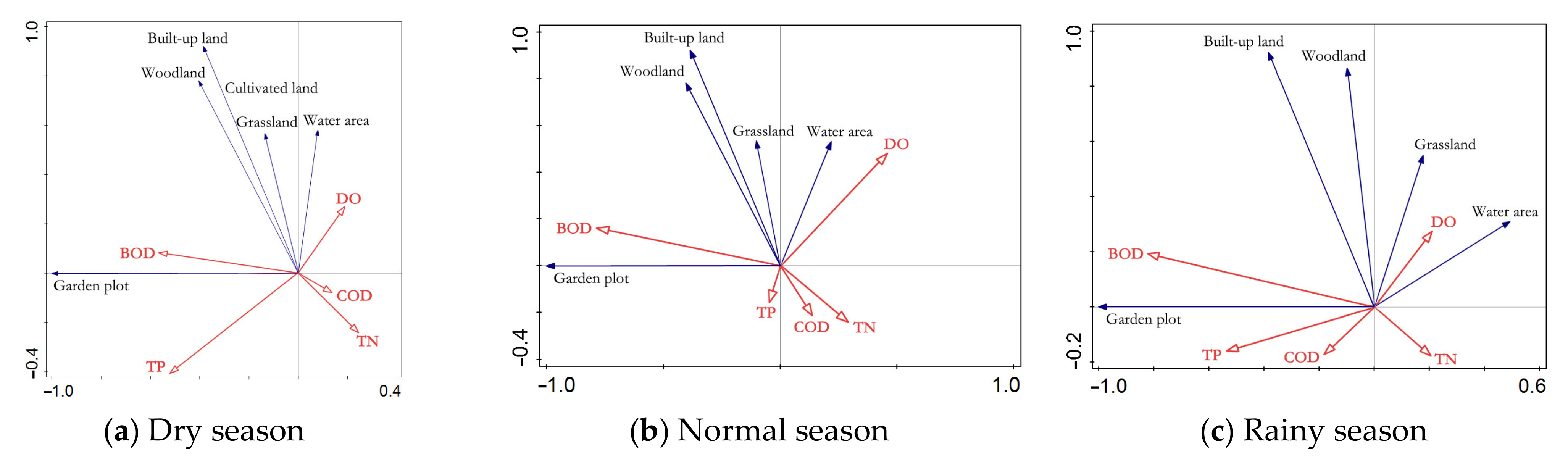
The TP in the dry season, DO in the dry and normal seasons, and COD in the rainy season were greatly affected by PD (adjusted R² > 0.5). Among them, the water area had a positive significant correlation with TP and a negative significant correlation with DO. Woodland was weakly correlated with water quality at different temporal and spatial scales. The garden plot had positive and negative significant correlations with TP and COD, respectively. Cultivated land had a positive significant correlation with TN, TP, and BOD, a highly significant positive correlation with COD, and a highly significant negative correlation with DO. Built-up land had a positive significant correlation with TN and TP and a negative significant correlation with DO.

The density of patches for cultivated land had a greater impact on water quality parameters in the rainy season than the rest of the year, with a greater density, resulting in worse water quality. The effect of season on the relationship between water area, garden plot, built-up land, and water quality remains unclear. In conclusion, the higher the PD, the worse the water quality and the higher the degree of fragmentation in the landscape (

Table 10. Multiple regression analysis between patch density and water quality.

Period	Index	Multivariate Regression Model	R2	Adjusted R2	P
Dry season	TP	0.120 + 0.005 built-up land	0.808	0.759	0.015
	DO	10.451 − 0.091 water area	0.792	0.723	0.043
Normal season	DO	8.530 − 0.475 cultivated land	0.861	0.815	0.023
Rainy season	COD	13.196 + 2.407 cultivated land	0.712	0.640	0.035

, Figure 15).

Correlation analysis was conducted between landscape shape (LSI) index and water quality parameters in different seasons. The results show that DO in dry and normal season and TP and COD in the rainy season were greatly affected by LSI (adjusted R² > 0.5). Among them, the water area is significantly negatively correlated with TP and COD and significantly positively correlated with DO. Woodland is significantly negatively correlated with TN and DO and extremely significantly positively correlated with TP. Garden plot is significantly positively correlated with TP, extremely significantly positively correlated with BOD, and extremely significantly negatively correlated with DO. Grassland is significantly positively correlated with TP and significantly negatively correlated with DO. Built-up land is significantly positively correlated with TN, COD, and BOD, extremely significantly positively correlated with TP, and significantly negatively correlated with DO.

The landscape shape of built-up land in the rainy season and grassland in the normal season had a significant negative effect on water quality parameters. The effect of season on the relationships between water area, woodland, garden plot, and water quality remains unclear. In conclusion, the higher the LSI of the water area, the better the water quality. The higher the LSI of garden plot, grassland, and built-up land, the worse the water quality. The higher the LSI of the woodland, the better the TN and COD, the worse the TP and DO (

Table 11. Multiple regression analysis between Landscape shape and water quality.

Period	Index	Multivariate Regression Model	R2	Adjusted R2	P
Dry season	DO	11.120 − 0.151 water area	0.865	0.820	0.022
Normal season	DO	9.479 − 0.118 grassland−0.081 built-up land	0.968	0.936	0.032
Rainy season	TP	0.043 + 0.007 built-up land	0.677	0.596	0.044
	BOD	7.192 + 0.779 garden plot	0.808	0.760	0.015

, Figure 16).

The TP in the dry and rainy seasons, BOD in all seasons, DO in the normal season, and TN in the rainy season were all greatly affected by LPI (adjusted R² > 0.5). Among them, the water area had a negative significant correlation with TP and COD and a positive significant correlation with DO. Woodland had a negative significant correlation with TN and DO and a highly significant positive correlation with TP. Garden plot had a positive significant correlation with DO and COD and a highly significant positive correlation with BOD. Cultivated land has a highly significant positive correlation with TN and TP and a positive significant correlation with COD. Built-up land had a positive significant correlation with TN, COD, and BOD, a highly significant negative correlation with TP, and a negative significant correlation with DO.

The maximum plaque of water area and woodland had a significant positive effect on water quality in the normal season. The seasonal effect on the relationship between garden plot and water quality remains unclear. In conclusion, the higher the LPI of water area and woodland, the better the water quality. The higher the LPI of the garden plot, the worse the DO and BOD, but the better the COD. The higher the LPI of cultivated land and built-up land, the worse the water quality (

Table 12. Multiple regression analysis between maximum plaque and water quality.

Period	Index	Multivariate Regression Model	R2	Adjusted R2	P
Dry season	TP	0.117 + 0.005 woodland	0.814	0.767	0.014
	BOD	11.930 + 4.944 grassland − 2.549 cultivated land	0.988	0.981	0.001
Normal season	DO	6.631 + 0.027 water area	0.770	0.693	0.051
	BOD	11.638 + 2.258 grassland	0.852	0.815	0.009
Rainy season	TN	1.213 + 0.480 cultivated land − 0.040 woodland	0.999	0.998	0.000
	TP	0.043 + 0.021 built-up land	0.781	0.726	0.019
	BOD	7.991 + 2.530 grassland	0.759	0.699	0.024

, Figure 17).

The TP in all seasons and the BOD in the normal and rainy seasons were greatly affected by AI (adjusted R² > 0.5). The water area had highly significant negative and positive correlations with TP and DO, respectively. Water area also had a negative significant correlation with COD and BOD. Woodland had a negative significant correlation with TN and TP. Garden plot had positive and negative significant correlations with TP and DO, respectively, as well as a highly significant negative correlation with BOD. Grassland had significant and highly significant negative correlations with TN and TP, respectively. Built-up land had a positive significant correlation with DO and was weakly correlated with the other water quality indices.

The effect of season on the relationships between water area, woodland, garden plot, grassland, and water quality remains unclear. There was no significant seasonal difference in the correlation between landscape patch aggregation and water quality. In conclusion, the higher the AI of water area, woodland, and grassland, the better the water quality (

Table 13. Multiple regression analysis between aggregation degree and water quality.

Period	Index	Multivariate Regression Model	R2	Adjusted R2	P
Dry season	TP	0.116 − 0.005 grassland	0.812	0.765	0.013
Normal season	TP	8.530 − 0.475 woodland	0.862	0.811	0.021
	BOD	10.930 + 4.642 garden plot − 2.458 water area	0.786	0.741	0.031
Rainy season	TP	8.279 − 0.082 water area	0.719	0.649	0.033
	BOD	7.089 + 0.059 garden plot	0.689	0.611	0.041

, Figure 18).

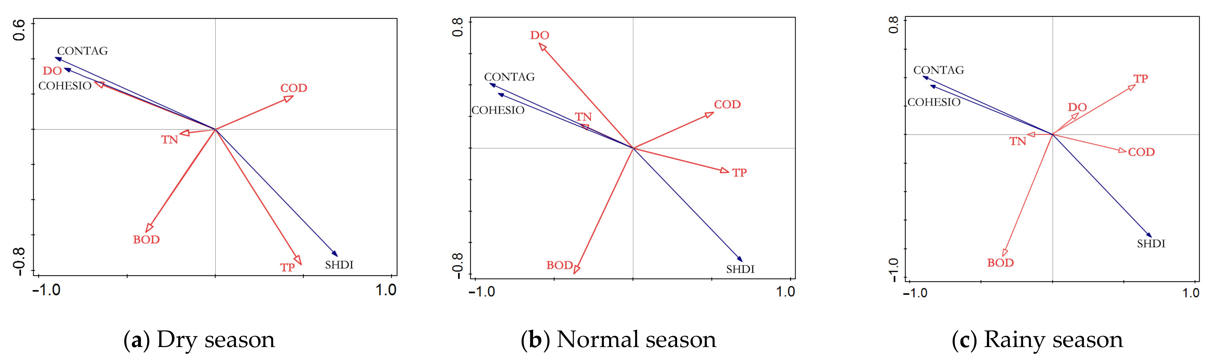
The TP in the rainy season, DO in dry and normal seasons, and COD in the rainy season were greatly affected by the landscape pattern index (adjusted R² > 0.5). Among them, the patch cohesion index (COHES) had highly significant negative and positive correlations with TP and DO, respectively. The contagion index (CONTAG) had a negative significant correlation with TP and COD and a positive significant correlation with DO. The Shannon’s diversity index (SHDI) had a positive significant correlation with TP and COD and a highly significant negative correlation with DO. In conclusion, the higher the COHES and CONTAG, the better the water quality. The higher the SHDI, the worse the water quality (

Table 14. Multiple regression analysis between landscape pattern index and water quality at the landscape level.

Period	Index	Multivariate Regression Model	R2	Adjusted R2	P
Dry season	DO	−493.146 + 5.038 COHESION	0.786	0.715	0.045
Normal season	DO	9.750 − 1.828 SHDI	0.889	0.852	0.016
Rainy season	TP	0.073 − 0.056 CONTAG	0.772	0.726	0.008
	COD	−174.642 + 113.475 SHDI	0.748	0.711	0.001

, Figure 19).

4. Discussion and Conclusions

4.1. Discussion

This paper used the “source-sink” theory to identify landscapes in the Suzhou National Wetland Park that act as a source and a sink for water quality pollution. Different landscape composition types and landscape spatial configurations affect hydrological processes and change the number of pollutants entering a waterway, resulting in the spatial differentiation of wetland water quality (

Table 15. “Source-sink” landscape judgment of Suzhou National Wetland Park.

Landscape Structure			Priority of Water Quality Improvement
			Level 1	Level 2	Level 3	Level 4	Level 5
			DO	TP	COD	TN	BOD
Composition Types	PLAND	sink	water	water	water, garden plot	woodland, garden plot	/
		source	woodland, garden plot, grassland, built-up land	woodland, grassland, built-up land	built-up land	built-up land	garden plot, built-up land
Spatial Configuration	NP	sink	/	/	/	/	/
		source	water, woodland, garden plot, built-up land	water, woodland, garden plot, cultivated land, built-up land	water, woodland, garden plot, cultivated land	water, garden plot, cultivated land, built-up land	garden plot, cultivated land
	PD	sink	/	/	garden plot	/	/
		source	water, cultivated land, built-up land	water, garden plot, cultivated land, built-up land	cultivated land	cultivated land, built-up land	cultivated land
	LSI	sink	water	water	water, woodland	woodland	/
		source	woodland, garden plot, grassland, built-up land	woodland, garden plot, grassland, built-up land	built-up land	built-up land	garden plot, built-up land
	LPI	sink	water	water	water, garden plot	woodland	/
		source	garden plot, built-up land	cultivated land, built-up land	cultivated land, built-up land	cultivated land, built-up land	garden plot, built-up land
	AI	sink	water, grassland	water, woodland, grassland	water	woodland, grassland	water
		source	garden plot	garden plot	/	/	garden plot

When a landscape type has two different landscape properties of source and sink for different water quality indices, the priority degree is adopted for judgment. The larger the number of 1–5, the higher the priority.

). It is concluded that the sink landscape was composed of water areas and woodland, where the larger the landscape pattern index, the better the water quality and the more pronounced the positive ecological effects. The source landscape was composed of cultivated and built-up land, where the larger the landscape index, the worse the water quality and the greater the negative ecological effect. Grasslands and garden plots had both source and sink characteristics, which was consistent with the findings from previous research [49,50]. However, unlike previous studies, the sink effect of grassland patches was not obvious because the area of grassland was relatively small [51,52]. The higher NP and PD in water and woodland patches and the increase of LSI in woodland patches were not conducive to the improvement of wetland water quality. As wetland parks are closed water systems, the decomposition of organic material along the bank may cause water pollution through surface runoff. This effect may be of particular concern in dry and normal seasons, when less rainfall, low water levels, and weak self-purification capacity can result in sedimentation and endogenous pollution [53,54].

4.2. Conclusions

In this study, Suzhou National Wetland Park was selected as the study site to explore the relationships between landscape structure characteristics and water quality. This work aimed to inform a new round of national wetland park planning and the rezoning of functional areas. The main research conclusions are as follows:

• The water quality of Suzhou National Wetland Parks ranked from good to bad was SSD > TH, SJB, HB > TL, TF. The seasonal effect on the correlation between landscape type and water quality ranked from strong to weak was rainy season > dry season > normal season. The purification effect of each landscape type arranged from large to small was water area, woodland > garden plot, grassland > cultivated land, built-up land. The pollutant parameters ranked from high to low were BOD > TN > COD > TP > DO. The landscape structure types arranged from good to bad were multi-layer cofferdam type > block-shaped agglomeration type > multi-pond structure type>block-like uniform type.
• In Suzhou National Wetland Park, the dominance and aggregation index of sink landscapes should be increased, and the fragmentation (except LSI) and diversity index of sink landscapes should be decreased. The aggregation index of source landscapes should be increased, and the fragmentation, dominance, and diversity index of source landscapes should be decreased.
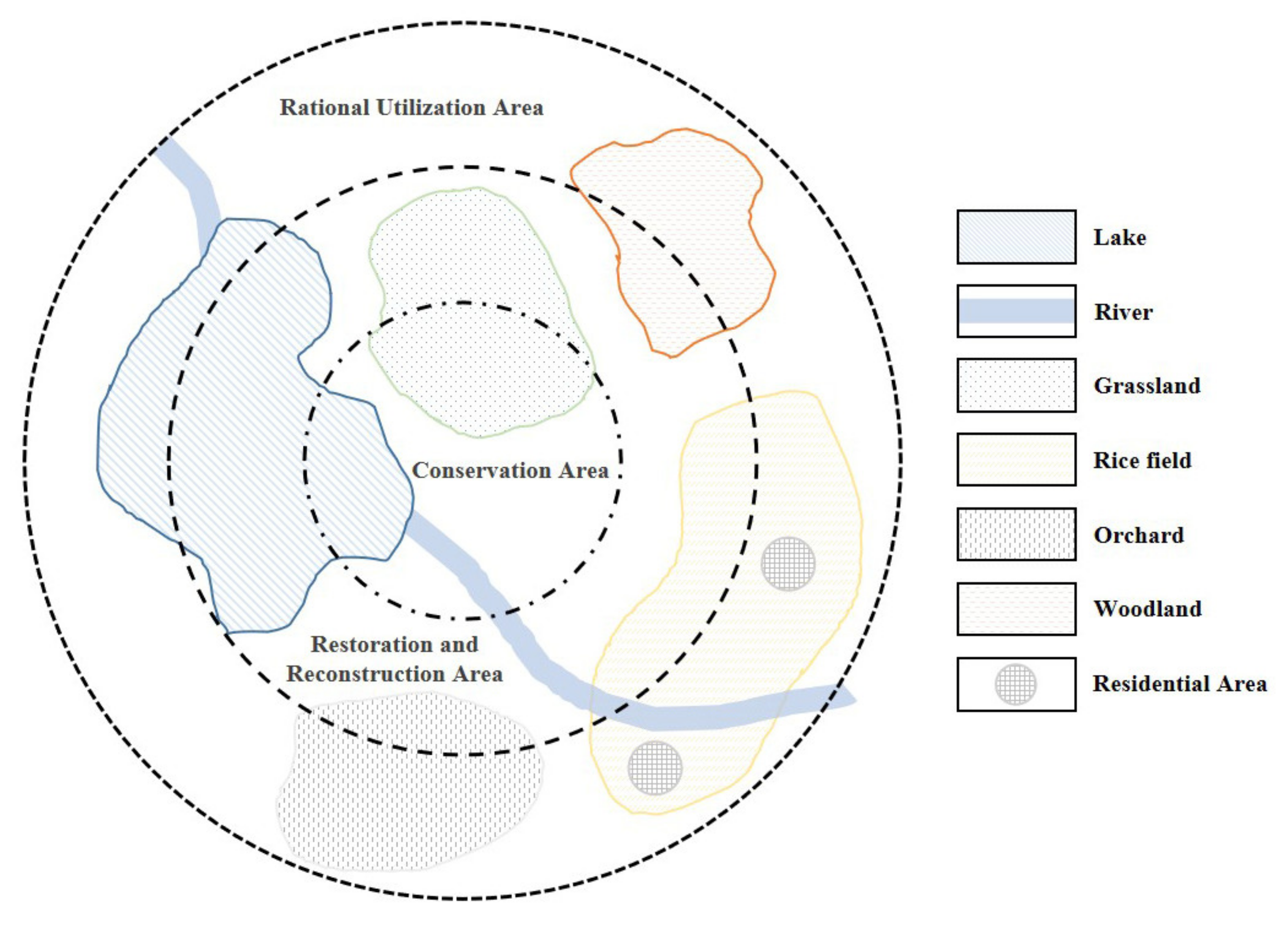
• As sink landscapes with good water quality and less disturbance, lakes can be included in conservation areas to improve ecosystem function. As an ecological corridor connecting the park to surrounding areas, the river should be located outside the core area. Upstream portions should remain some distance from the source landscape to control and manage the invasion of water pollution from internal and external sources. Herbaceous swamps provide habitat, breeding, and foraging places for birds, but as their ecology is fragile, they should be included in conservation, restoration, and/or reconstruction areas. To enhance the landscape heterogeneity and permeability of the wetland park, woodlands and grasslands can be used as buffer zones to separate water areas from garden plots and cultivated and built-up land. These buffers would also aid in the interception and emission reduction of pollutants through landscape structure adjustment. Areas close to roads and scenic spots in woodlands should be included in rational utilization areas for ornamental and tourist purposes. Built-up land, including residential areas, roads, infrastructures, etc. should also be included in rational utilization areas and kept far away from conservation areas to reduce the intrusion of pollutants (Figure 20).

4.

The overall water quality in Suzhou National Wetland Park was found to be good, contributing to its original intention for ecological conservation. However, there are still many problems, such as internal and external disturbance, single wetland habitat, and insufficient wetland reserve. Due to the fragile ecological landscape in the restoration and reconstruction area, measures such as setting a buffer zone, defining an interference zone, and controlling pollution sources should be taken. Rational utilization areas are subject to the most human impact and require increased efforts to control pollutants, appropriately reduce area, and realize the spatially intensive layout.

References

- Daily, G.C. Nature’s Services: Societal Dependence on Natural Ecosystem; Island Press: Washington, DC, USA, 1997. [Google Scholar]
- Barbier, E.B.; Acreman, M.; Knowler, D. Economic Valuation of Wetlands; Ramsar Convention Bureau: Gland, Switzerland, 1997; Available online: http://www.ramsar.org/sites/default/files/documents/pdf/lib/lib_valuation_e.pdf (accessed on 29 July 2021).
- Yang, Y. Main Characteristics, Progress and Prospect of International Wetland Science Research. Progr. Geogr. 2002, 21, 111–120. (In Chinese) [Google Scholar]
- Allan, C. Quebec 2000: Millennium Wetl. Event Program with Abstracts; Elizabeth MacKay: Quebec, QC, Canada, 2000; pp. 1–256. [Google Scholar]
- Fu, Y.; Zhao, J.; Peng, W.; Zhu, G.; Quan, Z.; Li, C. Spatial modelling of the regulating function of the Huangqihai Lake wetland ecosystem. J. Hydrol. 2018, 564, 283–293. [Google Scholar] [CrossRef]
- Wondie, A. Ecological conditions and ecosystem services of wetlands in the Lake Tana Area, Ethiopia. Ecohydrol. Hydrobiol. 2018, 18, 231–244. [Google Scholar] [CrossRef]
- Mitsch, W.J.; Gosselink, J.G. Wetls; Van Nostrand Reinhold Company Inc.: New York, NY, USA, 1986; pp. 22–38. [Google Scholar]
- Yan, F.; Zhang, S. Ecosystem service decline in response to wetland loss in the Sanjiang Plain, Northeast China. Ecol. Eng. 2019, 130, 117–121. [Google Scholar] [CrossRef]
- Hu, S.; Niu, Z.; Chen, Y.; Li, L.; Zhang, H. Global wetlands: Potential distribution, wetland loss, and status. Sci. Total Environ. 2017, 586, 319–327. [Google Scholar] [CrossRef]
- Han, D.Y.; Yang, Y.X.; Yang, Y.; Li, K. Progress in wetland degradation. Acta Ecol. Sin. 2012, 32, 289–303. (In Chinese) [Google Scholar]
- Somay, M.A. Importance of hydrogeochemical processes in the coastal wetlands: A case study from Edremit-Dalyan coastal wetland, Balocesses in the coastal wetlands: A case stogica. J. Afr. Earth Sci. 2012, 32, 4. [Google Scholar]
- Zhou, T.; Wu, J.; Peng, S. Assessing the effects of landscape pattern on river water quality at Multiple scales: A case study of the Dongjiang River watershed. China. Ecol. Indic. 2012, 23, 166–175. [Google Scholar] [CrossRef]
- Shokoufeh, S.; Almuktar, S.A.A.A.N.; Scholz, M. Impact of climate change on wetland ecosystems: A critical review of experimental wetlands. J. Environ. Manag. 2021, 286, 1–15. [Google Scholar]
- Jingbo, Z.; Jian, W.; Yazhen, G. Valuing wetland ecosystem services based on benefit transfer: A meta-analysis of China wetland studies. J. Clean. Prod. 2020, 276, 1–11. [Google Scholar]
- Gereta, E.; Mwangomo, E.; Wolanski, E. The influence of wetlands quality in the Seronera river, Serengeti national park, Tanzania. Wetl. Ecol. Manag. 2004, 12, 301–307. [Google Scholar] [CrossRef]
- Ahearn, D.S.; Sheibley, R.W.; Dahlgren, R.A.; Anderson, M.; Johnshon, J.; Tate, K.W. Land use and land cover influence on water quality in the last free-flowing river draining the western Sierra Nevada, California. J. Hydrol. 2005, 313, 234–247. [Google Scholar] [CrossRef]
- Mainali, J.; Chang, H. Landscape and anthropogenic factors affecting spatial patterns of water quality trends in a large river basin, South Korea. J. Hydrol. 2018, 564, 26–40. [Google Scholar] [CrossRef]
- Ho, H.L.; Edward, P.T.; Tran, N.T.; Nguyen, T.H.D.; Nguyen, T.C. An enhanced analytical framework of participatory GIS for ecosystem services assessment applied to a Ramsar wetland site in the Vietnam Mekong Delta. Ecosyst. Serv. 2021, 48, 1–11. [Google Scholar]
- Liu, H.; Li, Y.; Cao, X.; Hao, J.; Hu, J.; Zheng, J. The Current Problems and Perspectives of Landscape Research of Wetlands in China. Acta Geogr. Sin. 2009, 64, 1394–1401. [Google Scholar]
- Kwi, G.K.; Mi, Y.P.; Hee, S.C. Developing a wetland-type classification system in the Republic of Korea. Lands. Ecol. Eng. 2006, 2, 93–110. [Google Scholar]
- Zhou, D.; Gong, H.; Hu, J. Application of satellite remote sensing technology to wetland research. Remote Sens. Technol. Appl. 2006, 21, 577–581. (In Chinese) [Google Scholar]
- Li, X.; Bu, R.; Chang, Y.; Yunman, H.; Qingchun, W.; Xugao, W.; Chonggang, X.; Yuehui, L.; Hongshi, H. The response of landscape metrics against pattern scenarios. Acta Ecol. Sin. 2004, 24, 124–134. [Google Scholar]
- Yi, W.; Yang, L.; Zhang, Z. Remote Sensing Classification of Zharong Wetland Based on ETM+Image. Wetl. Sci. 2004, 22, 208–212. (In Chinese) [Google Scholar]
- Davranchea, A.; Lefebvreb, G.; Poulin, B. Wetland monitoring using classification trees and SPOT-5 seasonal time series. Remote Sens. Environ. 2010, 11414, 552–562. [Google Scholar] [CrossRef] [Green Version]
- Gong, H.L.; Jiao, C.C.; Zhou, D.M.; Li, N. Scale issues of wetland classification and mapping using remote sensing images: A case of Honghe National Nature Reserve in Sanjiang Plain, Northeast China. Chin. Geogr. Sci. 2011, 2121, 230–240. (In Chinese) [Google Scholar] [CrossRef]
- Herold, M.; Scepan, J.; Clarke, K.C. The use of remote sensing and landscape metrics to describe structures and changes in urban land uses. Environ. Plan. A 2002, 34, 1443–1458. [Google Scholar] [CrossRef] [Green Version]
- Wu, J. Landscape Ecology: Pattern, Process, Scale and Hierarchy; Higher Education Press: Beijing, China, 2007. [Google Scholar]
- Huang, S.; Guo, Q.H. Research review on effects of urban landscape pattern changes on water environment. Acta Ecol. Sin. 2014, 34, 3142–3150. [Google Scholar]
- Cui, D.; Chen, Y.M.B.; Bingram, M.A.; Weihua, Z.E.N.G.; Rui, L.I.; Zima, J.I.U. Effects of land use/landscape patterns on the water quality. Adv. Water Sci. 2019, 30, 423–433. (In Chinese) [Google Scholar]
- Lee, S.W.; Hwang, S.J.; Lee, S.B.; Huang, H.S.; Sung, H.C. Landscape ecological approach to the relationships of land use patterns in watersheds to water quality characteristics. Lands. Urban Plan. 2009, 92, 80–89. [Google Scholar] [CrossRef]
- Bahar, M.M.; Ohmori, H.; Yamamuro, M. Relationship between river water quality and land use in a small river basin running through the urbanizing area of Central Japan. Limnology 2008, 9, 19–26. [Google Scholar] [CrossRef]
- Xu, Q.; Wang, P.; Shu, W.; Ding, M.; Zhang, D. Influence of landscape structures on river water quality at multiple spatial scales: A case study of the Yuan river watershed, China. Ecol. Indic. 2021, 121, 1–11. [Google Scholar] [CrossRef]
- Chen, L.D.; Fu, B.J.; Zhao, W.W. Source-sink landscape theory and its ecological significance. Acta Ecol. Sin. 2006, 26, 1444–1449. [Google Scholar] [CrossRef]
- Basnyat, P.; Teeter, L.D.; Flynn, K.M.; Lockaby, G. Relationships between landscape characteristics and Non-point source pollution inputs to coastalestuary. Environ. Manag. 1999, 23, 539–549. [Google Scholar] [CrossRef]
- Alberti, M.; Booth, D.; Hill, K.; Coburn, K.; Avolio, C.; Coe, S.; Spirandelli, D. The impact of urban patterns on aquatic ecosystems: An empirical analysis in Puget lowland sub-basins. Lands. Urban Plan. 2007, 80, 345–361. [Google Scholar] [CrossRef]
- Huang, J.; Huang, Y.; Pontius, R.G.; Zhang, Z. Geographically weighted regression to measure spatial variations in correlations between water pollution versus land use in a coastal watershed. Ocean Coas. Manag. 2015, 103, 14–24. [Google Scholar] [CrossRef]
- Xu, G.; Ren, X.; Yang, Z.; Long, H.; Xiao, J. Influence of Landscape Structures on Water Quality at Multiple Temporal and Spatial Scales: A Case Study of Wujiang River Watershed in Guizhou. Water 2019, 11, 159. [Google Scholar] [CrossRef] [Green Version]
- Xia, L.L.; Liu, R.Z.; Zao, Y.W. Correlation analysis of landscape pattern and water quality in Baiyangdian Watershed. Proc. Environ. Sci. 2012, 13, 2188–2196. [Google Scholar] [CrossRef] [Green Version]
- Ding, J.; Jiang, Y.; Liu, Q.; Hou, Z.; Liao, J.; Fu, L.; Peng, Q. Influences of the land use pattern on water quality in low-order streams of the Dongjiang River basin, China: A multi-scale analysis. Sci. Total Environ. 2016, 551–552, 205–216. [Google Scholar] [CrossRef] [PubMed]
- Mello, K.D.; Valente, R.A.; Randhir, T.O.; dos Santos, A.C.A.; Vettorazzi, C.A. Effects of land use and land cover on water quality of low-order streams in Southeastern Brazil: Watershed versus riparian zone. Catena 2018, 167, 130–138. [Google Scholar] [CrossRef]
- Shi, P.; Zhang, Y.; Li, Z.; Peng, L.; Guoce, X. Influence of land use and land cover patterns on seasonal water quality at multi-spatial scales. Catena 2017, 151, 182–190. [Google Scholar] [CrossRef]
- Hille, S.; Andersen, D.K.; Kronvang, B.; Baattrup-Pedersen, A. Structural and functional characteristics of buffer strip vegetation in an agricultural landscape-high potential for nutrient removal but low potential for plant biodiversity. Sci. Total Environ. 2018, 628, 805–814. [Google Scholar] [CrossRef] [PubMed]
- Gong, D.; Hong, X.; Zeng, G.; Wang, I.; Zhuo, S.; Liu, X. Prediction of Water Quality in Rivers in Agricultural Regions Typical of Subtropics in China Using Multivariate Linear Regression Mode. J. Ecol. Rural Environ. 2017, 33, 509–518. [Google Scholar]
- Uuemaa, E.; Roosaare, J.; Mander, Ü. Scale dependence of landscape metrics and their indicatory value for nutrient and organic matter losses from catchments. Ecol. Indic. 2005, 5, 350–369. [Google Scholar] [CrossRef]
- McGarigal, K.; Marks, B. FRAGSTATS: Spatial Pattern Analysis Program for Quantifying Landscape Structure. Reference Manual; Forest Science Department, Oregon State University: Corvallis Oregon, OR, USA, 1994. [Google Scholar]
- Xu, Z. Single factor water quality identification index for environmental quality assessment of surface water. J. Tongji Univ. 2005, 33, 321–325. (In Chinese) [Google Scholar]
- Xu, Z. Comprehensive water quality identification index for environmental quality assessment of surface water. J. Tongji Univ. 2005, 33, 482–488. (In Chinese) [Google Scholar]
- Fan, J.; Mei, C. Data Analysis; Science Press: Beijing, China, 2006. (In Chinese) [Google Scholar]
- Tu, J. Spatially varying relationships between land use and water quality across an urbanization gradient explored by geographically weighted regression. Appl. Geogr. 2011, 31, 376–392. [Google Scholar] [CrossRef]
- Molinero, J.; Burke, R.A. Relations Between Land Use and Stream Nutrient Concentration for Small Watersheds in the Georgia Piedmont. In Proceedings of the 2003 Georgia Water Resources Conference, University of Georgia, Kathryn J. Institute of Ecology, Athens, Georgia, 23–24 April 2003. [Google Scholar]
- Jones, K.B.; Neale, A.C.; Nash, M.S.; Remortel, R.D.V.; Wickham, J.D.; Riitters, K.S.; O’Neill, R.V. Predicting nutrient and sediment loadings to streams from landscape metrics: A multiple watershed study from the United States Mid-Atlantic Region. Lands. Ecol. 2001, 16, 301–312. [Google Scholar] [CrossRef]
- Ge, F.; Huang, T.; Zhang, M.; Wang, X.F.; Xu, Z.F.; Yu, C. Effects of overwintering waterbirds on nitrogen and phosphorus in intermittent wetlands around Shengjin Lake. Chin. J. Ecol. 2018, 37, 3670–3675. (In Chinese) [Google Scholar]
- Cao, F.F.; Li, X.; Wang, D.; Zhao, Y.; Wang, Y.Q. Effect of land use structure on water quality in Xin′an River Basin. Environ. Sci. 2013, 34, 2582–2587. (In Chinese) [Google Scholar]
- Putro, B.; Kjeldsen, T.R.; Hutchins, M.G.; Miller, J. An empirical investigation of climate and land-use effects on water quantity and quality in two urbanising catchments in the southern United Kingdom. Sci. Total Environ. 2016, 548–549, 164–172. [Google Scholar] [CrossRef] [Green Version]
Figure 1.
Spatial distribution of waterways in the Suzhou Wetland Parks.
Figure 2.
Landscape types and distribution of sampling points in the Suzhou National Wetland Parks: (a) Taihu national wetland park (TH), (b) Shajiabang national wetland park (SJB), (c) Hubin national wetland park (HB), (d) Sanshan Island national wetland park (SSD), (e) Tianfu national wetland park (TF), (f) Tongli national wetland park (TL).
Figure 3.
The proportion of land cover classes of: (a) block-like uniform wetland parks, (b) multi-layer cofferdam wetland parks, (c) multi-pond structure wetland parks, (d) block-shaped agglomeration wetland parks.
Figure 4.
Differences in landscape pattern indices in Suzhou National Wetland Park.
Figure 5.
Average Pi value of TH sampling point.
Figure 6.
Average Pi value of SJB sampling point.
Figure 7.
Average Pi value of HB sampling point.
Figure 8.
Average Pi value of SSD sampling point.
Figure 9.
Average Pi value of TF sampling point.
Figure 10.
Average Pi value of TL sampling point.
Figure 11.
Analysis of water quality in different seasons by comprehensive water quality identification index method.
Figure 12.
Analysis of water quality in different functional zones by comprehensive water quality identification index method.
Figure 13.
Redundancy analysis ranking diagram of landscape area percentage and water quality index in (a) dry season, (b) normal season, (c) rainy season.
Figure 14.
Redundancy analysis ranking diagram of patch number (NP) and water quality index in (a) dry season, (b) normal season, (c) rainy season.
Figure 15.
Redundancy analysis ranking diagram of patches density (PD) and water quality index in (a) dry season, (b) normal season, (c) rainy season.
Figure 16.
Redundancy analysis ranking diagram of landscape shape index (LSI) and water quality index in (a) dry season, (b) normal season, (c) rainy season.
Figure 17.
Redundancy analysis ranking diagram of largest patch index (LPI) and water quality index in (a) dry season, (b) normal season, (c) rainy season.
Figure 18.
Redundancy analysis ranking diagram of aggregation index (AI) and water quality index in (a) dry season, (b) normal season, (c) rainy season.
Figure 19.
Redundancy analysis ranking diagram of landscape pattern index and water quality index at the landscape level in (a) dry season, (b) normal season, (c) rainy season.
Figure 20.
Functional zoning strategy of wetland park landscape types.