MLE-Based Parameter Estimation for Four-Parameter Exponential Gamma Distribution and Asymptotic Variance of Its Quantiles

Abstract

The choice of a probability distribution function and confidence interval of estimated design values have long been of interest in flood frequency analysis. Although the four-parameter exponential gamma (FPEG) distribution has been developed for application in hydrology, its maximum likelihood estimation (MLE)-based parameter estimation method and asymptotic variance of its quantiles have not been well documented. In this study, the MLE method was used to estimate the parameters and confidence intervals of quantiles of the FPEG distribution. This method entails parameter estimation and asymptotic variances of quantile estimators. The parameter estimation consisted of a set of four equations which, after algebraic simplification, were solved using a three dimensional Levenberg-Marquardt algorithm. Based on sample information matrix and Fisher’s expected information matrix, derivatives of the design quantile with respect to the parameters were derived. The method of estimation was applied to annual precipitation data from the Weihe watershed, China and confidence intervals for quantiles were determined. Results showed that the FPEG was a good candidate to model annual precipitation data and can provide guidance for estimating design values.

1. Introduction

Hydrological frequency analysis is important for planning, designing and managing water resources projects. The design values (e.g., design flood, design rainfall) computed by frequency analysis involve uncertainties due to the sampling method, sample length, empirical frequency formula, cumulative distribution function (CDF) or probability density function (PDF), parameter estimation method, goodness-of-fit test, and extent of data extrapolation [1,2]. Among these uncertainty sources, there has been a considerable interest in the choice of CDF for a given sample, because the true CDF of a hydrological variable is unknown. Rao and Hamed summarized commonly used distributions: normal and related, gamma family, extreme value, Wakeby, and logistic as well as their application [3].

Further, quantifying the uncertainty of the estimated design values is important in the planning, design, and management of water resources projects [1,4]. In practice, standard error and confidence interval (confidence limits) are employed to measure the uncertainty of a statistical quantity [4]. Rao and Hamed provided confidence intervals of some common distributions, with parameters estimated by the method of moments (MOM), the probability weighted moments (PWM), and maximum likelihood estimation (MLE) [3]. Shin [5] and Shin et al. [6] summarized methods for computing confidence intervals. Methods of estimating the confidence intervals of design quantities include Monte Carlo simulation [7], approximate method [8], analytical method [5,9,10,11], asymptotic variance of the expected moments algorithm [12], bootstrap method [13,14,15,16], and standard error of regional population index flood (RPIF) [17]. Studies show that confidence intervals mainly depend on the method of estimation of the parameters of the probability distribution function.

The four-parameter exponential gamma (FPEG) distribution has been applied in hydrology in China and be specialized into 10 kinds of probability distribution functions: gamma, Pearson type III (P-III), K–M, Weibull, Chi-square, exponential, normal, Pearson type V (P-V), log-normal, and Gumbel. The properties of FPEG distribution and relations between this distribution and others, and its potential for application, have been investigated [18,19]. However, the MLE-based parameter estimation method and algorithms for computing confidence intervals of the design values for the FPEG distribution have received little attention.

The objective of this paper, therefore, is to present the MLE method for estimating the FPEG distribution parameters, and derive confidence intervals of quantiles using asymptotic variances. The method of parameter estimation involved a set of four equations which are solved by a three dimensional Levenberg–Marquardt algorithm. Following Kendall and Stuart [20], the expected values of the second-order partial derivatives of the log-likelihood function with respect to the parameters, and the explicit formulae for the variances and covariances are analytically derived. The proposed estimation procedure is illustrated by using observed annual precipitation data.

The paper is organized as follows. Describing the FPEG distribution and estimation of its quantiles. A set of four equations of the MLE method for parameters and confidence intervals of quantiles are derived in Section 2, followed by an application to annual precipitation from the Weihe watershed in China in Section 3. Conclusions, along with a summary of the main features of the proposed method, are given in Section 4.

2. Theory and Methodology

2.1. Probability Density Function and Cumulative Distribution Function

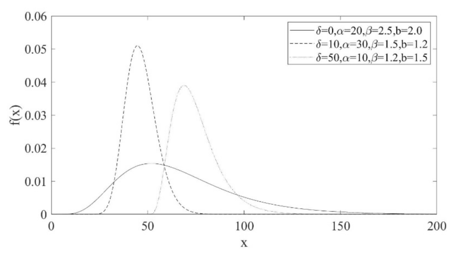
The FPEG distribution has the probability density function (PDF), f(x), expressed as [18,19]:

$$f\left(x\right)=\left\{\begin{array}{ccc}\frac{{\beta }^{\alpha }}{b\mathsf{\Gamma }\left(\alpha \right)}{\left(x-\delta \right)}^{\frac{\alpha }{b}-1}{e}^{-\beta {\left(x-\delta \right)}^{\frac{1}{b}}}& ;& \delta \le x<\infty \\ 0& ;& \mathrm{otherwise}\end{array}\right.$$

(1)

where $\alpha >0$ is the shape parameter; $\beta >0$ is the scale parameter; $\delta >0$ is the location parameter; $b>0$ is the transformation parameter; $\mathsf{\Gamma }\left(\alpha \right)$ is the complete gamma function; x is the value of the random variable X. Figure 1 shows some typical shapes of the PDF. The CDF can be expressed as

$$p=F\left(X\le x\right)={{\displaystyle \int }}_{\delta }^{x}f\left(t\right)dt={{\displaystyle \int }}_{\delta }^x\frac{{\beta }^{\alpha }}{b\mathsf{\Gamma }\left(\alpha \right)}{\left(t-\delta \right)}^{\frac{\alpha }{b}-1}{e}^{-\beta {\left(t-\delta \right)}^{\frac{1}{b}}}dt$$

When the design frequency $p$ is given, its correspondance to design value $x_p$ (quantile) can be expressed as

$$p=F\left(X\le x_p\right)={{\displaystyle \int }}_{\delta }^{x_p}f\left(x\right)dx={{\displaystyle \int }}_{\delta }^{x_p}\frac{{\beta }^{\alpha }}{b\mathsf{\Gamma }\left(\alpha \right)}{\left(x-\delta \right)}^{\frac{\alpha }{b}-1}{e}^{-\beta {\left(x-\delta \right)}^{\frac{1}{b}}}dx$$

(2)

Equation (2) can be transformed to a one-parameter gamma using the following transformation. Let $t=\beta {\left(x-\delta \right)}^{\frac{1}{b}}$, then $x=\delta +\frac{1}{{\beta }^b}{t}^b$, $x-\delta =\frac{1}{{\beta }^b}{t}^b$ and $dx=\frac{b}{{\beta }^b}{t}^{b-1}dt$, when $x=\delta$, $t=0$; $x=x_p$, $t_p=\beta {\left(x_p-\delta \right)}^{\frac{1}{b}}$ substitution of these quantities into Equation (2) results in [18,19]:

$$p={{\displaystyle \int }}_0^{t_p}\frac{{\beta }^{\alpha }}{b\mathsf{\Gamma }\left(\alpha \right)}{\left(\frac{1}{{\beta }^b}{t}^b\right)}^{\frac{\alpha }{b}-1}{e}^{-t}\frac{b}{{\beta }^b}{t}^{b-1}dt={{\displaystyle \int }}_0^{t_p}\frac{{\beta }^{\alpha }}{b\mathsf{\Gamma }\left(\alpha \right)}\frac{1}{{\beta }^{\alpha -b}}{t}^{\alpha -b}{e}^{-t}\frac{b}{{\beta }^b}{t}^{b-1}dt={{\displaystyle \int }}_0^{t_p}\frac{1}{\mathsf{\Gamma }\left(\alpha \right)}{t}^{\alpha -1}{e}^{-t}dt$$

(3)

where $t_p=\beta {\left(x_p-\delta \right)}^{\frac{1}{b}}$, which can be determined by the incomplete gamma function.

2.2. Estimation of Quantiles

The quantile corresponding to the probability of exceedance $p$, $x_p$, is obtained as

$$x_p=\delta +\frac{1}{{\beta }^b}{t}_p^b$$

(4)

Also, the estimator $x_p$ may be generally written in terms of the mathematical expectation $E\left(X\right)$, the coefficient of variation $C_v$, and the frequency factor ${\mathsf{\Phi }}_p$ as

$$x_p=E\left(X\right)\left(1+{\mathsf{\Phi }}_p{C}_v\right)$$

(5)

Given the probability of exceedance $p$, the frequency factor ${\mathsf{\Phi }}_p$ can be written in the following form [18,19]:

$${\mathsf{\Phi }}_p=\frac{t_p^b\mathsf{\Gamma }\left(\alpha \right)-\mathsf{\Gamma }\left(\alpha +b\right)}{\sqrt{\mathsf{\Gamma }\left(\alpha \right)\mathsf{\Gamma }\left(\alpha +2b\right)-{\mathsf{\Gamma }}^2\left(\alpha +b\right)}}$$

(6)

Note that from Equations (3) and (6), the frequency factor ${\mathsf{\Phi }}_p$ is a function of the probability of exceedance and parameters $\alpha$ and $b$. Some numerical values for such a function are shown in

Table 1. Frequency factors for the four-parameter exponential gamma distribution.

$\mathit{b}=0.50$
$\mathit{\alpha }$	$\mathbf{Exceedance}\mathbf{Probability}\mathit{p}$
	0.001	0.01	0.02	0.10	0.30	0.50	0.70	0.90	0.95	0.99	0.995	0.999
0.10	6.1052	4.0173	3.2803	1.3079	−0.0892	−0.4810	−0.5628	−0.5697	−0.5697	−0.5697	−0.5697	−0.5697
0.20	5.0293	3.4670	2.9186	1.4286	0.1880	−0.4003	−0.7010	−0.8087	−0.8147	−0.8160	−0.8160	−0.8160
0.30	4.5665	3.2055	2.7291	1.4308	0.3045	−0.3081	−0.7170	−0.9631	−0.9950	−1.0087	−1.0094	−1.0097
0.40	4.3045	3.0513	2.6134	1.4183	0.3625	−0.2462	−0.7029	−1.0574	−1.1260	−1.1691	−1.1729	−1.1753
0.50	4.1350	2.9494	2.5356	1.4050	0.3957	−0.2047	−0.6844	−1.1151	−1.2196	−1.3028	−1.3132	−1.3215
0.60	4.0161	2.8770	2.4796	1.3934	0.4168	−0.1757	−0.6676	−1.1516	−1.2869	−1.4136	−1.4332	−1.4518
0.70	3.9278	2.8228	2.4375	1.3835	0.4312	−0.1545	−0.6534	−1.1755	−1.3362	−1.5050	−1.5355	−1.5679
0.80	3.8596	2.7807	2.4046	1.3753	0.4416	−0.1385	−0.6417	−1.1920	−1.3732	−1.5807	−1.6225	−1.6713
0.90	3.8051	2.7470	2.3782	1.3684	0.4494	−0.1259	−0.6320	−1.2037	−1.4017	−1.6438	−1.6967	−1.7632
1.00	3.7605	2.7193	2.3565	1.3625	0.4555	−0.1159	−0.6239	−1.2124	−1.4242	−1.6967	−1.7602	−1.8448
2.00	3.5423	2.5845	2.2506	1.3323	0.4817	−0.0701	−0.5840	−1.2436	−1.5195	−1.9561	−2.0881	−2.3133
4.00	3.4078	2.5032	2.1871	1.3141	0.4955	−0.0455	−0.5617	−1.2564	−1.5655	−2.0975	−2.2754	−2.6114
6.00	3.3513	2.4699	2.1614	1.3070	0.5010	−0.0361	−0.5534	−1.2611	−1.5823	−2.1492	−2.3442	−2.7233
8.00	3.3179	2.4506	2.1466	1.3031	0.5041	−0.0308	−0.5488	−1.2638	−1.5917	−2.1773	−2.3815	−2.7840
10.00	3.2951	2.4375	2.1366	1.3005	0.5062	−0.0273	−0.5459	−1.2656	−1.5978	−2.1955	−2.4056	−2.8229
20.00	3.2380	2.4054	2.1123	1.2945	0.5115	−0.0190	−0.5390	−1.2702	−1.6123	−2.2377	−2.4610	−2.9117
40.00	3.1966	2.3827	2.0953	1.2905	0.5152	−0.0133	−0.5344	−1.2734	−1.6221	−2.2653	−2.4971	−2.9686
60.00	3.1779	2.3726	2.0878	1.2887	0.5168	−0.0108	−0.5325	−1.2749	−1.6263	−2.2770	−2.5123	−2.9924
80.00	3.1666	2.3665	2.0833	1.2877	0.5178	−0.0094	−0.5314	−1.2757	−1.6288	−2.2839	−2.5212	−3.0063
100.00	3.1588	2.3623	2.0802	1.2871	0.5185	−0.0084	−0.5306	−1.2763	−1.6305	−2.2885	−2.5272	−3.0156
200.00	3.1392	2.3519	2.0725	1.2854	0.5202	−0.0059	−0.5288	−1.2778	−1.6348	−2.2998	−2.5418	−3.0382
400.00	3.1251	2.3445	2.0670	1.2843	0.5214	−0.0042	−0.5275	−1.2789	−1.6377	−2.3077	−2.5520	−3.0538
600.00	3.1188	2.3412	2.0646	1.2838	0.5220	−0.0034	−0.5269	−1.2794	−1.6390	−2.3112	−2.5564	−3.0606
800.00	3.1151	2.3392	2.0632	1.2835	0.5223	−0.0029	−0.5266	−1.2797	−1.6398	−2.3132	−2.5590	−3.0646
1000.00	3.1125	2.3379	2.0622	1.2833	0.5225	−0.0026	−0.5263	−1.2799	−1.6404	−2.3146	−2.5608	−3.0674
$\mathit{b}=1.00$
$\alpha$	$\mathrm{Exceedance}\mathrm{Probability}\mathit{p}$
	0.001	0.01	0.02	0.10	0.30	0.50	0.70	0.90	0.95	0.99	0.995	0.999
0.10	10.3207	4.7070	3.2225	0.5254	−0.2611	−0.3144	−0.3162	−0.3162	−0.3162	−0.3162	−0.3162	−0.3162
0.20	8.7251	4.4773	3.2969	0.9054	−0.1766	−0.4008	−0.4437	−0.4472	−0.4472	−0.4472	−0.4472	−0.4472
0.30	7.8853	4.2712	3.2435	1.0677	−0.0793	−0.4142	−0.5245	−0.5471	−0.5477	−0.5477	−0.5477	−0.5477
0.40	7.3406	4.1111	3.1792	1.1540	−0.0043	−0.4031	−0.5731	−0.6287	−0.6318	−0.6324	−0.6325	−0.6325
0.50	6.9491	3.9845	3.1197	1.2060	0.0525	−0.3854	−0.6021	−0.6959	−0.7043	−0.7070	−0.7071	−0.7071
0.60	6.6497	3.8815	3.0671	1.2400	0.0965	−0.3670	−0.6197	−0.7513	−0.7673	−0.7741	−0.7744	−0.7746
0.70	6.4109	3.7957	3.0209	1.2635	0.1316	−0.3497	−0.6305	−0.7970	−0.8221	−0.8352	−0.8361	−0.8366
0.80	6.2145	3.7229	2.9802	1.2804	0.1601	−0.3339	−0.6371	−0.8352	−0.8699	−0.8912	−0.8931	−0.8942
0.90	6.0493	3.6601	2.9442	1.2930	0.1839	−0.3197	−0.6410	−0.8673	−0.9118	−0.9426	−0.9459	−0.9482
1.00	5.9078	3.6052	2.9120	1.3026	0.2040	−0.3069	−0.6433	−0.8946	−0.9487	−0.9899	−0.9950	−0.9990
2.00	5.1148	3.2798	2.7110	1.3362	0.3106	−0.2274	−0.6383	−1.0382	−1.1629	−1.3092	−1.3410	−1.3821
4.00	4.5311	3.0226	2.5421	1.3404	0.3811	−0.1640	−0.6181	−1.1276	−1.3168	−1.5884	−1.6639	−1.7857
6.00	4.2681	2.9020	2.4605	1.3369	0.4105	−0.1347	−0.6054	−1.1627	−1.3827	−1.7207	−1.8220	−1.9975
8.00	4.1105	2.8284	2.4100	1.3332	0.4274	−0.1169	−0.5967	−1.1822	−1.4210	−1.8010	−1.9194	−2.1316
10.00	4.0026	2.7775	2.3748	1.3301	0.4387	−0.1048	−0.5904	−1.1949	−1.4466	−1.8562	−1.9869	−2.2261
20.00	3.7345	2.6487	2.2848	1.3198	0.4656	−0.0743	−0.5733	−1.2242	−1.5083	−1.9941	−2.1571	−2.4690
40.00	3.5449	2.5558	2.2191	1.3106	0.4838	−0.0526	−0.5601	−1.2429	−1.5502	−2.0918	−2.2791	−2.6468
60.00	3.4610	2.5142	2.1894	1.3060	0.4916	−0.0430	−0.5539	−1.2507	−1.5683	−2.1351	−2.3334	−2.7269
80.00	3.4111	2.4893	2.1716	1.3031	0.4962	−0.0372	−0.5502	−1.2552	−1.5789	−2.1608	−2.3658	−2.7749
100.00	3.3770	2.4723	2.1593	1.3011	0.4993	−0.0333	−0.5476	−1.2582	−1.5861	−2.1784	−2.3880	−2.8079
200.00	3.2927	2.4298	2.1288	1.2957	0.5068	−0.0236	−0.5410	−1.2655	−1.6037	−2.2219	−2.4430	−2.8900
400.00	3.2332	2.3996	2.1070	1.2918	0.5121	−0.0167	−0.5362	−1.2704	−1.6159	−2.2526	−2.4819	−2.9483
600.00	3.2069	2.3862	2.0973	1.2900	0.5144	−0.0136	−0.5341	−1.2725	−1.6213	−2.2661	−2.4991	−2.9743
800.00	3.1912	2.3782	2.0915	1.2889	0.5157	−0.0118	−0.5328	−1.2737	−1.6245	−2.2742	−2.5094	−2.9898
1000.00	3.1806	2.3727	2.0875	1.2881	0.5167	−0.0105	−0.5319	−1.2746	−1.6267	−2.2797	−2.5164	−3.0003
$\mathit{b}=1.50$
$\alpha$	$\mathrm{Exceedance}\mathrm{Probability}\mathit{p}$
	0.001	0.01	0.02	0.10	0.30	0.50	0.70	0.90	0.95	0.99	0.995	0.999
0.10	12.8886	4.0481	2.3121	0.0921	−0.1944	−0.1992	−0.1993	−0.1993	−0.1993	−0.1993	−0.1993	−0.1993
0.20	11.5995	4.3915	2.8159	0.3898	−0.2229	−0.2788	−0.2830	−0.2831	−0.2831	−0.2831	−0.2831	−0.2831
0.30	10.7500	4.4459	2.9974	0.5824	−0.2028	−0.3260	−0.3465	−0.3481	−0.3481	−0.3481	−0.3481	−0.3481
0.40	10.1286	4.4298	3.0780	0.7137	−0.1704	−0.3519	−0.3965	−0.4032	−0.4033	−0.4033	−0.4033	−0.4033
0.50	9.6438	4.3907	3.1154	0.8089	−0.1367	−0.3652	−0.4360	−0.4516	−0.4521	−0.4522	−0.4522	−0.4522
0.60	9.2498	4.3439	3.1311	0.8810	−0.1049	−0.3713	−0.4673	−0.4949	−0.4963	−0.4966	−0.4966	−0.4966
0.70	8.9202	4.2953	3.1349	0.9377	−0.0758	−0.3729	−0.4923	−0.5338	−0.5368	−0.5376	−0.5376	−0.5376
0.80	8.6385	4.2474	3.1318	0.9833	−0.0495	−0.3719	−0.5125	−0.5689	−0.5741	−0.5758	−0.5759	−0.5759
0.90	8.3938	4.2013	3.1245	1.0208	−0.0256	−0.3693	−0.5290	−0.6007	−0.6085	−0.6117	−0.6119	−0.6120
1.00	8.1783	4.1573	3.1147	1.0521	−0.0040	−0.3656	−0.5426	−0.6295	−0.6405	−0.6456	−0.6460	−0.6461
2.00	6.8717	3.8286	2.9915	1.2080	0.1351	−0.3192	−0.6040	−0.8156	−0.8645	−0.9074	−0.9141	−0.9206
4.00	5.8088	3.4886	2.8158	1.2896	0.2518	−0.2547	−0.6233	−0.9689	−1.0757	−1.2040	−1.2335	−1.2744
6.00	5.3092	3.3073	2.7105	1.3131	0.3060	−0.2171	−0.6220	−1.0377	−1.1801	−1.3709	−1.4207	−1.4975
8.00	5.0061	3.1907	2.6395	1.3224	0.3383	−0.1923	−0.6179	−1.0777	−1.2442	−1.4806	−1.5464	−1.6537
10.00	4.7981	3.1076	2.5876	1.3266	0.3602	−0.1743	−0.6136	−1.1043	−1.2884	−1.5596	−1.6381	−1.7706
20.00	4.2817	2.8908	2.4471	1.3286	0.4131	−0.1268	−0.5971	−1.1664	−1.3981	−1.7689	−1.8857	−2.0978
40.00	3.9208	2.7297	2.3388	1.3226	0.4487	−0.0909	−0.5806	−1.2060	−1.4743	−1.9263	−2.0762	−2.3604
60.00	3.7632	2.6569	2.2887	1.3178	0.4638	−0.0746	−0.5719	−1.2221	−1.5072	−1.9981	−2.1641	−2.4847
80.00	3.6702	2.6131	2.2583	1.3144	0.4725	−0.0647	−0.5664	−1.2313	−1.5266	−2.0413	−2.2175	−2.5610
100.00	3.6071	2.5830	2.2373	1.3118	0.4784	−0.0580	−0.5625	−1.2373	−1.5397	−2.0710	−2.2543	−2.6140
200.00	3.4523	2.5082	2.1845	1.3045	0.4926	−0.0411	−0.5522	−1.2516	−1.5716	−2.1452	−2.3467	−2.7485
400.00	3.3444	2.4550	2.1467	1.2985	0.5023	−0.0291	−0.5445	−1.2611	−1.5936	−2.1980	−2.4131	−2.8462
600.00	3.2971	2.4314	2.1298	1.2957	0.5065	−0.0238	−0.5410	−1.2651	−1.6032	−2.2215	−2.4427	−2.8902
800.00	3.2690	2.4174	2.1197	1.2939	0.5090	−0.0206	−0.5388	−1.2674	−1.6089	−2.2355	−2.4604	−2.9166
1000.00	3.2499	2.4078	2.1128	1.2927	0.5106	−0.0184	−0.5374	−1.2690	−1.6128	−2.2451	−2.4725	−2.9346
$\mathit{b}=2.00$
$\alpha$	$\mathrm{Exceedance}\mathrm{Probability}\mathit{p}$
	0.001	0.01	0.02	0.10	0.30	0.50	0.70	0.90	0.95	0.99	0.995	0.999
0.10	13.3536	2.8762	1.3613	−0.0467	−0.1307	−0.1311	−0.1311	−0.1311	−0.1311	−0.1311	−0.1311	−0.1311
0.20	12.9833	3.6087	2.0068	0.0986	−0.1764	−0.1875	−0.1879	−0.1879	−0.1879	−0.1879	−0.1879	−0.1879
0.30	12.4989	3.9246	2.3406	0.2345	−0.1935	−0.2295	−0.2326	−0.2327	−0.2327	−0.2327	−0.2327	−0.2327
0.40	12.0542	4.0914	2.5456	0.3473	−0.1950	−0.2612	−0.2708	−0.2714	−0.2714	−0.2714	−0.2714	−0.2714
0.50	11.6592	4.1868	2.6831	0.4409	−0.1884	−0.2851	−0.3039	−0.3062	−0.3062	−0.3062	−0.3062	−0.3062
0.60	11.3083	4.2425	2.7802	0.5195	−0.1777	−0.3030	−0.3330	−0.3379	−0.3381	−0.3381	−0.3381	−0.3381
0.70	10.9946	4.2742	2.8512	0.5864	−0.1650	−0.3164	−0.3585	−0.3674	−0.3677	−0.3677	−0.3677	−0.3677
0.80	10.7121	4.2903	2.9041	0.6440	−0.1512	−0.3266	−0.3811	−0.3949	−0.3955	−0.3956	−0.3956	−0.3956
0.90	10.4561	4.2962	2.9442	0.6942	−0.1371	−0.3342	−0.4010	−0.4206	−0.4217	−0.4220	−0.4220	−0.4220
1.00	10.2227	4.2949	2.9748	0.7383	−0.1231	−0.3398	−0.4188	−0.4447	−0.4466	−0.4472	−0.4472	−0.4472
2.00	8.6475	4.1535	3.0588	0.9962	−0.0055	−0.3473	−0.5233	−0.6238	−0.6409	−0.6522	−0.6535	−0.6544
4.00	7.1806	3.8570	2.9806	1.1743	0.1277	−0.3106	−0.5893	−0.8083	−0.8645	−0.9212	−0.9319	−0.9447
6.00	6.4445	3.6576	2.8918	1.2401	0.1994	−0.2775	−0.6084	−0.9033	−0.9909	−1.0934	−1.1167	−1.1487
8.00	5.9875	3.5177	2.8205	1.2724	0.2448	−0.2520	−0.6148	−0.9620	−1.0735	−1.2150	−1.2501	−1.3022
10.00	5.6704	3.4134	2.7637	1.2907	0.2765	−0.2322	−0.6165	−1.0023	−1.1326	−1.3066	−1.3522	−1.4232
20.00	4.8774	3.1261	2.5947	1.3204	0.3559	−0.1746	−0.6103	−1.0998	−1.2855	−1.5637	−1.6459	−1.7877
40.00	4.3242	2.9025	2.4527	1.3260	0.4104	−0.1275	−0.5957	−1.1635	−1.3957	−1.7697	−1.8885	−2.1063
60.00	4.0846	2.7994	2.3846	1.3240	0.4336	−0.1052	−0.5865	−1.1895	−1.4440	−1.8665	−2.0047	−2.2643
80.00	3.9440	2.7371	2.3427	1.3215	0.4471	−0.0916	−0.5801	−1.2042	−1.4724	−1.9256	−2.0764	−2.3635
100.00	3.8491	2.6942	2.3136	1.3192	0.4560	−0.0822	−0.5754	−1.2139	−1.4916	−1.9666	−2.1263	−2.4332
200.00	3.6181	2.5870	2.2396	1.3115	0.4776	−0.0585	−0.5625	−1.2365	−1.5385	−2.0698	−2.2532	−2.6137
400.00	3.4588	2.5107	2.1861	1.3044	0.4921	−0.0415	−0.5523	−1.2511	−1.5708	−2.1440	−2.3456	−2.7474
600.00	3.3894	2.4769	2.1621	1.3008	0.4983	−0.0339	−0.5476	−1.2572	−1.5848	−2.1772	−2.3871	−2.8083
800.00	3.3484	2.4567	2.1478	1.2985	0.5020	−0.0294	−0.5446	−1.2608	−1.5930	−2.1970	−2.4120	−2.8450
1000.00	3.3205	2.4429	2.1379	1.2969	0.5044	−0.0263	−0.5426	−1.2631	−1.5987	−2.2106	−2.4291	−2.8702
$\mathit{b}=2.50$
$\alpha$	$\mathrm{Exceedance}\mathrm{Probability}\mathit{p}$
	0.001	0.01	0.02	0.10	0.30	0.50	0.70	0.90	0.95	0.99	0.995	0.999
0.10	12.0692	1.7751	0.6880	−0.0666	−0.0880	−0.0880	−0.0880	−0.0880	−0.0880	−0.0880	−0.0880	−0.0880
0.20	12.7687	2.5964	1.2456	−0.0196	−0.1254	−0.1273	−0.1273	−0.1273	−0.1273	−0.1273	−0.1273	−0.1273
0.30	12.8544	3.0532	1.6046	0.0500	−0.1496	−0.1586	−0.1590	−0.1591	−0.1591	−0.1591	−0.1591	−0.1591
0.40	12.7678	3.3500	1.8603	0.1209	−0.1643	−0.1851	−0.1868	−0.1869	−0.1869	−0.1869	−0.1869	−0.1869
0.50	12.6164	3.5586	2.0536	0.1881	−0.1725	−0.2076	−0.2120	−0.2123	−0.2123	−0.2123	−0.2123	−0.2123
0.60	12.4387	3.7119	2.2053	0.2503	−0.1761	−0.2269	−0.2350	−0.2358	−0.2358	−0.2358	−0.2358	−0.2358
0.70	12.2515	3.8278	2.3275	0.3075	−0.1764	−0.2434	−0.2563	−0.2580	−0.2580	−0.2580	−0.2580	−0.2580
0.80	12.0630	3.9171	2.4277	0.3599	−0.1744	−0.2575	−0.2760	−0.2790	−0.2790	−0.2790	−0.2790	−0.2790
0.90	11.8772	3.9868	2.5112	0.4081	−0.1708	−0.2696	−0.2942	−0.2989	−0.2991	−0.2991	−0.2991	−0.2991
1.00	11.6965	4.0417	2.5815	0.4524	−0.1660	−0.2801	−0.3111	−0.3180	−0.3183	−0.3184	−0.3184	−0.3184
2.00	10.2326	4.2145	2.9186	0.7530	−0.0967	−0.3301	−0.4289	−0.4725	−0.4779	−0.4807	−0.4809	−0.4810
4.00	8.5558	4.0896	3.0201	1.0138	0.0227	−0.3331	−0.5308	−0.6614	−0.6890	−0.7126	−0.7163	−0.7201
6.00	7.6256	3.9254	2.9892	1.1268	0.1006	−0.3139	−0.5718	−0.7717	−0.8230	−0.8757	−0.8860	−0.8988
8.00	7.0250	3.7892	2.9406	1.1878	0.1541	−0.2938	−0.5915	−0.8444	−0.9163	−0.9979	−1.0159	−1.0403
10.00	6.6000	3.6791	2.8931	1.2250	0.1931	−0.2760	−0.6019	−0.8961	−0.9854	−1.0937	−1.1193	−1.1562
20.00	5.5168	3.3486	2.7229	1.2952	0.2960	−0.2165	−0.6133	−1.0273	−1.1736	−1.3789	−1.4358	−1.5289
40.00	4.7541	3.0720	2.5591	1.3206	0.3698	−0.1617	−0.6056	−1.1166	−1.3157	−1.6225	−1.7159	−1.8812
60.00	4.4248	2.9407	2.4762	1.3243	0.4016	−0.1346	−0.5974	−1.1535	−1.3793	−1.7409	−1.8552	−2.0641
80.00	4.2324	2.8606	2.4242	1.3242	0.4200	−0.1177	−0.5911	−1.1745	−1.4169	−1.8142	−1.9426	−2.1814
100.00	4.1031	2.8052	2.3877	1.3231	0.4323	−0.1058	−0.5862	−1.1882	−1.4424	−1.8654	−2.0040	−2.2651
200.00	3.7900	2.6660	2.2939	1.3169	0.4618	−0.0757	−0.5717	−1.2200	−1.5046	−1.9958	−2.1625	−2.4853
400.00	3.5763	2.5666	2.2252	1.3095	0.4815	−0.0539	−0.5596	−1.2405	−1.5474	−2.0907	−2.2794	−2.6519
600.00	3.4838	2.5225	2.1943	1.3054	0.4899	−0.0441	−0.5538	−1.2489	−1.5660	−2.1333	−2.3323	−2.7285
800.00	3.4293	2.4961	2.1757	1.3028	0.4948	−0.0382	−0.5502	−1.2538	−1.5769	−2.1589	−2.3642	−2.7750
1000.00	3.3925	2.4782	2.1630	1.3009	0.4981	−0.0342	−0.5476	−1.2570	−1.5843	−2.1764	−2.3861	−2.8071

. For large $\alpha$ (e.g., $\alpha >100$) it is seen that the differences among the ${\mathsf{\Phi }}_p$ values for a given $p$ are subtle.

2.3. Maximum Likelihood Estimation of the Parameters

For the maximum likelihood estimation (MLE), the log-likelihood function for a sample $x=\left\{x_1,x_2,\cdots ,x_n\right\}$ drawn from the FPEG distribution can be written as

$$ln\left(L\right)=n\alpha ln\beta -nlnb-nln\mathsf{\Gamma }\left(\alpha \right)+\frac{\alpha }{b}{\displaystyle \sum }_{i=1}^{n}ln\left(x_i-\delta \right)-{\displaystyle \sum }_{i=1}^{n}ln\left(x_i-\delta \right)-\beta {\displaystyle \sum }_{i=1}^n{\left(x_i-\delta \right)}^{\frac{1}{b}}$$

(7)

where $n$ is the sample size, $\delta \le x<\infty$; $\alpha >0$; $\beta >0$.

The MLE parameters can be obtained by taking the derivatives of the log likelihood with respect to parameters, setting them equal to zero, and solving for the parameters. Differentiating Equation (7) partially with respect to each parameter and equating each partial derivative to zero yield

$$-\frac{\alpha }{b}{\displaystyle \sum }_{i=1}^n\frac{1}{x_i-\delta }+{\displaystyle \sum }_{i=1}^n\frac{1}{x_i-\delta }+\frac{\beta }{b}{\displaystyle \sum }_{i=1}^n{\left(x_i-\delta \right)}^{\frac{1}{b}-1}=0$$

(8)

$$nln\beta -n\mathsf{\Psi }\left(\alpha \right)+\frac{1}{b}{\displaystyle \sum }_{i=1}^{n}ln\left(x_i-\delta \right)=0$$

(9)

where $\mathsf{\Psi }\left(\alpha \right)$ is the digamma function.

$$\frac{n\alpha }{\beta }-{\displaystyle \sum }_{i=1}^n{\left(x_i-\delta \right)}^{\frac{1}{b}}=0$$

(10)

$$-\frac{n}{b}-\frac{\alpha }{b^2}{\displaystyle \sum }_{i=1}^{n}ln\left(x_i-\delta \right)+\frac{\beta }{b^2}{\displaystyle \sum }_{i=1}^n\left[{\left(x_i-\delta \right)}^{\frac{1}{b}}ln\left(x_i-\delta \right)\right]=0$$

(11)

Equations (8)–(11) can be solved numerically to obtain parameters $\widehat{\alpha }$, $\widehat{\beta }$, $\widehat{\delta }$, and $\widehat{b}$.

2.4. Confidence Intervals of Quantiles

For a given $p$, the design value estimate $x_p$ is a random variable. The 1 − q confidence intervals for the population quantiles $x_p$ may be determined by [2,3]

$$x_p^L=x_p-u_{1-q/2}S\left(x_p\right), x_p^U=x_p+u_{1-q/2}S\left(x_p\right)$$

(12)

where $u_{1-q/2}$ is the $1-q/2$ quantile of the standard normal distribution, $x_p$ is the quantile estimator corresponding to the probability of exceedance $p$ which can be determined from Equation (4) or Equation (5), and $S\left(x_p\right)$ is the standard deviation or standard error of $x_p$. Such standard error $S\left(x_p\right)$ determined by the MLE is given in what follows.

For the FPEG distribution, when parameters $\alpha$, $\beta$, $\delta$, and $b$ are estimated by the MLE, $x_p$ is a function of $\alpha$, $\beta$, $\delta$, and $b$:

$$x_p=x_p\left(\alpha ,\beta ,\delta ,b,p\right)$$

(13)

The variance in this case is given by [21]

$$Var\left(x_p\right)={\left(\frac{\partial x_p}{\partial \delta }\right)}^{2}Var\left(\delta \right)+{\left(\frac{\partial x_p}{\partial \alpha }\right)}^{2}Var\left(\alpha \right)+{\left(\frac{\partial x_p}{\partial \beta }\right)}^{2}Var\left(\beta \right)+{\left(\frac{\partial x_p}{\partial b}\right)}^{2}Var\left(b\right)$$

$$+2\frac{\partial x_p}{\partial \delta }\frac{\partial x_p}{\partial \alpha }Cov\left(\delta ,\alpha \right)+2\frac{\partial x_p}{\partial \delta }\frac{\partial x_p}{\partial \beta }Cov\left(\delta ,\beta \right)+2\frac{\partial x_p}{\partial \delta }\frac{\partial x_p}{\partial b}Cov\left(\delta ,b\right)$$

$$+2\frac{\partial x_p}{\partial \alpha }\frac{\partial x_p}{\partial \beta }Cov\left(\alpha ,\beta \right)+2\frac{\partial x_p}{\partial \alpha }\frac{\partial x_p}{\partial b}Cov\left(\alpha ,b\right)+2\frac{\partial x_p}{\partial \beta }\frac{\partial x_p}{\partial b}Cov\left(\beta ,b\right)$$

(14)

The variance and covariance matrix of parameters in Equation (13) is the inverse of Fisher’s expected information matrix [3].

$$\left[\begin{array}{cccc}Var\left(\delta \right)& Cov\left(\delta ,\alpha \right)& Cov\left(\delta ,\beta \right)& Cov\left(\delta ,b\right)\\ Cov\left(\alpha ,\delta \right)& Var\left(\alpha \right)& Cov\left(\alpha ,\beta \right)& Cov\left(\alpha ,b\right)\\ Cov\left(\beta ,\delta \right)& Cov\left(\beta ,\alpha \right)& Var\left(\beta \right)& Cov\left(\beta ,b\right)\\ Cov\left(b,\delta \right)& Cov\left(b,\alpha \right)& Cov\left(b,\beta \right)& Var\left(b\right)\end{array}\right]$$

$$=\left[\begin{array}{c}E\left(-\frac{{\partial }^2\mathit{ln}L}{\partial {\delta }^2}\right)E\left(-\frac{{\partial }^2\mathit{ln}L}{\partial \delta \partial \alpha }\right)E\left(-\frac{{\partial }^2\mathit{ln}L}{\partial \delta \partial \beta }\right)E\left(-\frac{{\partial }^2\mathit{ln}L}{\partial \delta \partial b}\right)\\ E\left(-\frac{{\partial }^2\mathit{ln}L}{\partial \alpha \partial \delta }\right)E\left(-\frac{{\partial }^2\mathit{ln}L}{\partial {\alpha }^2}\right)E\left(-\frac{{\partial }^2\mathit{ln}L}{\partial \alpha \partial \beta }\right)E\left(-\frac{{\partial }^2\mathit{ln}L}{\partial \alpha \partial b}\right)\\ E\left(-\frac{{\partial }^2\mathit{ln}L}{\partial \beta \partial \delta }\right)E\left(-\frac{{\partial }^2\mathit{ln}L}{\partial \beta \partial \alpha }\right)E\left(-\frac{{\partial }^2\mathit{ln}L}{\partial {\beta }^2}\right)E\left(-\frac{{\partial }^2\mathit{ln}L}{\partial \beta \partial b}\right)\\ E\left(-\frac{{\partial }^2\mathit{ln}L}{\partial b\partial \delta }\right)E\left(-\frac{{\partial }^2\mathit{ln}L}{\partial b\partial \alpha }\right)E\left(-\frac{{\partial }^2\mathit{ln}L}{\partial b\partial \beta }\right)E\left(-\frac{{\partial }^2\mathit{ln}L}{\partial b^2}\right)\end{array}\right]$$

(15)

where E represents the expected value;

$$\left[\begin{array}{cccc}-\frac{{\partial }^{2}lnL}{\partial {\delta }^2}& -\frac{{\partial }^{2}lnL}{\partial \delta \partial \alpha }& -\frac{{\partial }^{2}lnL}{\partial \delta \partial \beta }& -\frac{{\partial }^{2}lnL}{\partial \delta \partial b}\\ -\frac{{\partial }^{2}lnL}{\partial \alpha \partial \delta }& -\frac{{\partial }^{2}lnL}{\partial {\alpha }^2}& -\frac{{\partial }^{2}lnL}{\partial \alpha \partial \beta }& -\frac{{\partial }^{2}lnL}{\partial \alpha \partial b}\\ -\frac{{\partial }^{2}lnL}{\partial \beta \partial \delta }& -\frac{{\partial }^{2}lnL}{\partial \beta \partial \alpha }& -\frac{{\partial }^{2}lnL}{\partial {\beta }^2}& -\frac{{\partial }^{2}lnL}{\partial \beta \partial b}\\ -\frac{{\partial }^{2}lnL}{\partial b\partial \delta }& -\frac{{\partial }^{2}lnL}{\partial b\partial \alpha }& -\frac{{\partial }^{2}lnL}{\partial b\partial \beta }& -\frac{{\partial }^{2}lnL}{\partial b^2}\end{array}\right]$$

is the sample information matrix;

$$\left[\begin{array}{c}E\left(-\frac{{\partial }^2\mathit{ln}L}{\partial {\delta }^2}\right)E\left(-\frac{{\partial }^2\mathit{ln}L}{\partial \delta \partial \alpha }\right)E\left(-\frac{{\partial }^2\mathit{ln}L}{\partial \delta \partial \beta }\right)E\left(-\frac{{\partial }^2\mathit{ln}L}{\partial \delta \partial b}\right)\\ E\left(-\frac{{\partial }^2\mathit{ln}L}{\partial \alpha \partial \delta }\right)E\left(-\frac{{\partial }^2\mathit{ln}L}{\partial {\alpha }^2}\right)E\left(-\frac{{\partial }^2\mathit{ln}L}{\partial \alpha \partial \beta }\right)E\left(-\frac{{\partial }^2\mathit{ln}L}{\partial \alpha \partial b}\right)\\ E\left(-\frac{{\partial }^2\mathit{ln}L}{\partial \beta \partial \delta }\right)E\left(-\frac{{\partial }^2\mathit{ln}L}{\partial \beta \partial \alpha }\right)E\left(-\frac{{\partial }^2\mathit{ln}L}{\partial {\beta }^2}\right)E\left(-\frac{{\partial }^2\mathit{ln}L}{\partial \beta \partial b}\right)\\ E\left(-\frac{{\partial }^2\mathit{ln}L}{\partial b\partial \delta }\right)E\left(-\frac{{\partial }^2\mathit{ln}L}{\partial b\partial \alpha }\right)E\left(-\frac{{\partial }^2\mathit{ln}L}{\partial b\partial \beta }\right)E\left(-\frac{{\partial }^2\mathit{ln}L}{\partial b^2}\right)\end{array}\right]$$

is Fisher’s expected information matrix, the elements of which can be determined by taking the expected value of the sample information matrix. Its elements are derived in Equations (A1)–(A16) and Equations (A17)–(A32) in Appendix A, respectively.

$$E\left(-\frac{{\partial }^{2}lnL}{\partial {\delta }^2}\right)=\frac{\alpha -2b+b^2}{b^2}·\frac{n{\beta }^{2b}\mathsf{\Gamma }\left(\alpha -2b\right)}{\mathsf{\Gamma }\left(\alpha \right)}$$

(16)

$$E\left(-\frac{{\partial }^{2}lnL}{\partial \delta \partial \alpha }\right)=\frac{1}{b}·\frac{n{\beta }^b\mathsf{\Gamma }\left(\alpha -b\right)}{\mathsf{\Gamma }\left(\alpha \right)}$$

(17)

$$E\left(-\frac{{\partial }^{2}lnL}{\partial \delta \partial \beta }\right)=-\frac{\left(\alpha -b\right)}{b}·\frac{n{\beta }^{b-1}\mathsf{\Gamma }\left(\alpha -b\right)}{\mathsf{\Gamma }\left(\alpha \right)}$$

(18)

$$E\left(-\frac{{\partial }^{2}lnL}{\partial \delta \partial b}\right)=-\frac{1}{b}·\frac{n{\beta }^b\mathsf{\Gamma }\left(\alpha -b\right)}{\mathsf{\Gamma }\left(\alpha \right)}+\frac{1}{b^2}\frac{n{\beta }^b}{\mathsf{\Gamma }\left(\alpha \right)}\left[\frac{\partial \mathsf{\Gamma }\left(\alpha -b+1\right)}{\partial \left(\alpha -b+1\right)}-ln\beta ·\mathsf{\Gamma }\left(\alpha -b+1\right)\right]$$

(19)

$$E\left(-\frac{{\partial }^{2}lnL}{\partial \alpha \partial \delta }\right)=E\left(-\frac{{\partial }^{2}lnL}{\partial \delta \partial \alpha }\right)$$

(20)

$$E\left(-\frac{{\partial }^{2}lnL}{\partial {\alpha }^2}\right)=n{\mathsf{\Psi }}^{\prime }\left(\alpha \right)$$

(21)

$$E\left(-\frac{{\partial }^{2}lnL}{\partial \alpha \partial \beta }\right)=-\frac{n}{\beta }$$

(22)

$$E\left(-\frac{{\partial }^{2}lnL}{\partial \alpha \partial b}\right)=\frac{n\left[-ln\beta +\mathsf{\Psi }\left(\alpha \right)\right]}{b}$$

(23)

$$E\left(-\frac{{\partial }^{2}lnL}{\partial \beta \partial \delta }\right)=E\left(-\frac{{\partial }^{2}lnL}{\partial \delta \partial \beta }\right)$$

(24)

$$E\left(-\frac{{\partial }^{2}lnL}{\partial \beta \partial \alpha }\right)=E\left(-\frac{{\partial }^{2}lnL}{\partial \alpha \partial \beta }\right)$$

(25)

$$E\left(-\frac{{\partial }^{2}lnL}{\partial {\beta }^2}\right)=\frac{n\alpha }{{\beta }^2}$$

(26)

$$E\left(-\frac{{\partial }^{2}lnL}{\partial \beta \partial b}\right)=-\frac{n}{b\beta }·\frac{\frac{\partial \mathsf{\Gamma }\left(\alpha +1\right)}{\partial \left(\alpha +1\right)}-ln\beta ·\mathsf{\Gamma }\left(\alpha +1\right)}{\mathsf{\Gamma }\left(\alpha \right)}$$

(27)

$$E\left(-\frac{{\partial }^{2}lnL}{\partial b\partial \delta }\right)=E\left(-\frac{{\partial }^{2}lnL}{\partial \delta \partial b}\right)$$

(28)

$$E\left(-\frac{{\partial }^{2}lnL}{\partial b\partial \alpha }\right)=E\left(-\frac{{\partial }^{2}lnL}{\partial \alpha \partial b}\right)$$

(29)

$$E\left(-\frac{{\partial }^{2}lnL}{\partial b\partial \beta }\right)=E\left(-\frac{{\partial }^{2}lnL}{\partial \beta \partial b}\right)$$

(30)

$$E\left(-\frac{{\partial }^{2}lnL}{\partial b^2}\right)=-\frac{n}{b^2}-\frac{2n\alpha \left[-ln\beta +\mathsf{\Psi }\left(\alpha \right)\right]}{b^2}+\frac{2}{b^2}\frac{n\left[\frac{\partial \mathsf{\Gamma }\left(\alpha +1\right)}{\partial \left(\alpha +1\right)}-ln\beta ·\mathsf{\Gamma }\left(\alpha +1\right)\right]}{\mathsf{\Gamma }\left(\alpha \right)}$$

$$+\frac{1}{b^2}\frac{n}{\mathsf{\Gamma }\left(\alpha \right)}\left[\frac{{\partial }^2\mathsf{\Gamma }\left(\alpha +1\right)}{\partial {\left(\alpha +1\right)}^2}-2ln\frac{\partial \mathsf{\Gamma }\left(\alpha +1\right)}{\partial \left(\alpha +1\right)}+{\left(ln\beta \right)}^2·\mathsf{\Gamma }\left(\alpha +1\right)\right]$$

(31)

The derivatives of $x_p$ with respect to the parameters of the FPEG distribution are obtained from Equation (4) as

$$\frac{\partial x_p}{\partial \delta }=1$$

(32)

$$\frac{\partial x_p}{\partial \alpha }=\frac{b}{{\beta }^b}{t}_p^{b-1}\frac{\partial t_p}{\partial \alpha }$$

(33)

$$\frac{\partial x_p}{\partial \beta }=-\frac{b}{{\beta }^{b+1}}{t}_p^b$$

(34)

$$\frac{\partial x_p}{\partial b}=-\frac{1}{{\beta }^b}ln\beta ·t_p^b+\frac{1}{{\beta }^b}{t}_p^{b}ln{t}_p$$

(35)

For $\frac{\partial x_p}{\partial \alpha }$ in Equation (33), $p$ is a constant and is a function of $t_p$ and $\alpha$ in Equation (3). Thus, we can get $\frac{\partial p}{\partial t_p}\frac{\partial t_p}{\partial \alpha }+\frac{\partial p}{\partial \alpha }=0$, which reduces to

$$\frac{\partial t_p}{\partial \alpha }=-\frac{\partial p}{\partial \alpha }/\frac{\partial p}{\partial t_p}$$

(36)

$$\frac{\partial p}{\partial t_p}=\frac{1}{\mathsf{\Gamma }\left(\alpha \right)}{t}_p^{\alpha -1}{e}^{-t_p}$$

(37)

$$\frac{\partial p}{\partial \alpha }=-\frac{{\mathsf{\Gamma }}^{\prime }\left(\alpha \right)}{{\mathsf{\Gamma }}^2\left(\alpha \right)}{{\displaystyle \int }}_0^{t_p}{t}^{\alpha -1}{e}^{-t}dt+\frac{1}{\mathsf{\Gamma }\left(\alpha \right)}{{\displaystyle \int }}_0^{t_p}{t}^{\alpha -1}{e}^{-t}lntdt=-\mathsf{\Psi }\left(\alpha \right)\mathsf{\gamma }\left(t_p,\alpha \right)+\frac{1}{\mathsf{\Gamma }\left(\alpha \right)}{{\displaystyle \int }}_0^{t_p}{t}^{\alpha -1}{e}^{-t}lntdt$$

(38)

where $\mathsf{\Psi }\left(\alpha \right)=\frac{{\mathsf{\Gamma }}^{\prime }\left(\alpha \right)}{{\mathsf{\Gamma }}^2\left(\alpha \right)}$ is the psi function with a different meaning in Equation (9); $\mathsf{\gamma }\left(t_p,\alpha \right)=\frac{1}{\mathsf{\Gamma }\left(\alpha \right)}{{\displaystyle \int }}_0^{t_p}{t}^{\alpha -1}{e}^{-t}dt$ is the incomplete gamma function; ${{\displaystyle \int }}_0^{t_p}{t}^{\alpha -1}{e}^{-t}lntdt$ can be numerically calculated by the central difference of ${{\displaystyle \int }}_0^{t_p}{t}^{\alpha -1}{e}^{-t}dt$. Some $\frac{1}{\mathsf{\Gamma }\left(\alpha \right)}{{\displaystyle \int }}_0^{t_p}{t}^{\alpha -1}{e}^{-t}lntdt$ values obtained numerically are listed in

Table 2. $\frac{1}{\mathsf{\Gamma }\left(\alpha \right)}{{\displaystyle \int }}_0^{t_p}{t}^{\alpha -1}{e}^{-t}lnt·dt$ values under different probabilities of exceedance $p$.

$\mathit{\alpha }$	$\mathbf{Exceedance} \mathbf{Probability} \mathit{p}$
	0.001	0.01	0.02	0.10	0.30	0.50	0.70	0.90	0.95	0.99	0.995	0.999
0.10	−10.4252	−10.4319	−10.4346	−10.3799	−9.8448	−8.7151	−6.7615	−3.3525	−2.0228	−0.5655	−0.3174	−0.0796
0.20	−5.2906	−5.2998	−5.3062	−5.3012	−5.0361	−4.4449	−3.4340	−1.6940	−1.0203	−0.2845	−0.1596	−0.0400
0.30	−3.5042	−3.5148	−3.5232	−3.5425	−3.3894	−2.9959	−2.3115	−1.1369	−0.6840	−0.1904	−0.1068	−0.0267
0.40	−2.5632	−2.5747	−2.5845	−2.6200	−2.5347	−2.2519	−1.7404	−0.8555	−0.5144	−0.1431	−0.0802	−0.0201
0.50	−1.9653	−1.9777	−1.9886	−2.0361	−1.9990	−1.7906	−1.3900	−0.6845	−0.4116	−0.1145	−0.0642	−0.0161
0.60	−1.5425	−1.5556	−1.5673	−1.6246	−1.6247	−1.4713	−1.1502	−0.5688	−0.3423	−0.0953	−0.0534	−0.0134
0.70	−1.2220	−1.2356	−1.2481	−1.3136	−1.3439	−1.2340	−0.9737	−0.4847	−0.2921	−0.0814	−0.0457	−0.0114
0.80	−0.9670	−0.9811	−0.9944	−1.0668	−1.1227	−1.0485	−0.8371	−0.4204	−0.2539	−0.0709	−0.0398	−0.0100
0.90	−0.7570	−0.7716	−0.7854	−0.8641	−0.9420	−0.8981	−0.7273	−0.3694	−0.2237	−0.0627	−0.0352	−0.0088
1.00	−0.5793	−0.5943	−0.6087	−0.6930	−0.7903	−0.7726	−0.6365	−0.3277	−0.1992	−0.0560	−0.0315	−0.0079
2.00	0.4205	0.4024	0.3841	0.2622	0.0411	−0.0998	−0.1628	−0.1194	−0.0788	−0.0242	−0.0139	−0.0036
3.00	0.9203	0.9002	0.8795	0.7345	0.4422	0.2155	0.0509	−0.0314	−0.0295	−0.0119	−0.0072	−0.0020
4.00	1.2535	1.2319	1.2093	1.0474	0.7045	0.4186	0.1857	0.0223	−0.0001	−0.0048	−0.0034	−0.0011
5.00	1.5033	1.4805	1.4565	1.2811	0.8988	0.5675	0.2834	0.0603	0.0206	0.0001	−0.0008	−0.0005
6.00	1.7032	1.6794	1.6541	1.4675	1.0528	0.6848	0.3597	0.0894	0.0363	0.0037	0.0011	−0.0001
7.00	1.8698	1.8450	1.8187	1.6224	1.1802	0.7813	0.4220	0.1130	0.0489	0.0066	0.0027	0.0002
8.00	2.0126	1.9870	1.9597	1.7550	1.2888	0.8633	0.4747	0.1327	0.0594	0.0090	0.0039	0.0005
9.00	2.1375	2.1112	2.0830	1.8708	1.3834	0.9344	0.5202	0.1497	0.0683	0.0110	0.0050	0.0008
10.00	2.2486	2.2216	2.1926	1.9736	1.4671	0.9972	0.5602	0.1645	0.0762	0.0127	0.0059	0.0010
20.00	2.9669	2.9353	2.9010	2.6357	2.0024	1.3952	0.8111	0.2554	0.1237	0.0231	0.0112	0.0021
30.00	3.3805	3.3460	3.3084	3.0150	2.3062	1.6189	0.9504	0.3049	0.1493	0.0286	0.0140	0.0027
40.00	3.6722	3.6356	3.5955	3.2817	2.5189	1.7748	1.0469	0.3388	0.1667	0.0323	0.0159	0.0031
50.00	3.8976	3.8594	3.8174	3.4876	2.6826	1.8944	1.1206	0.3645	0.1799	0.0350	0.0173	0.0034
60.00	4.0815	4.0418	3.9983	3.6553	2.8157	1.9913	1.1802	0.3852	0.1905	0.0372	0.0184	0.0036
70.00	4.2367	4.1959	4.1509	3.7967	2.9277	2.0729	1.2303	0.4025	0.1993	0.0391	0.0194	0.0038
80.00	4.3710	4.3291	4.2830	3.9190	3.0244	2.1432	1.2734	0.4174	0.2069	0.0406	0.0202	0.0040
90.00	4.4894	4.4466	4.3994	4.0267	3.1096	2.2050	1.3112	0.4305	0.2135	0.0420	0.0209	0.0041
100.00	4.5952	4.5516	4.5035	4.1229	3.1856	2.2601	1.3449	0.4420	0.2194	0.0432	0.0215	0.0042
200.00	5.2903	5.2410	5.1866	4.7540	3.6826	2.6197	1.5640	0.5170	0.2573	0.0510	0.0254	0.0050
300.00	5.6962	5.6436	5.5853	5.1219	3.9715	2.8280	1.6904	0.5599	0.2791	0.0554	0.0277	0.0055
400.00	5.9841	5.9290	5.8680	5.3825	4.1758	2.9752	1.7796	0.5901	0.2943	0.0585	0.0292	0.0058
500.00	6.2072	6.1503	6.0872	5.5845	4.3340	3.0890	1.8485	0.6134	0.3060	0.0609	0.0304	0.0061
600.00	6.3896	6.3311	6.2662	5.7494	4.4631	3.1818	1.9046	0.6324	0.3155	0.0629	0.0314	0.0063
700.00	6.5437	6.4839	6.4176	5.8887	4.5722	3.2601	1.9519	0.6483	0.3236	0.0645	0.0322	0.0064
800.00	6.6772	6.6162	6.5486	6.0094	4.6665	3.3279	1.9929	0.6621	0.3305	0.0659	0.0329	0.0066
900.00	6.7949	6.7329	6.6642	6.1158	4.7497	3.3876	2.0289	0.6743	0.3366	0.0671	0.0335	0.0067
1000.00	6.9002	6.8374	6.7676	6.2110	4.8241	3.4410	2.0611	0.6851	0.3421	0.0682	0.0341	0.0068

.

Finally, the expression of $\frac{\partial t_p}{\partial \alpha }$ in Equation (33) can be obtained by substituting Equations (37) and (38) into Equation (36).

Table 3. Values under different probabilities of exceedance $p$ .

$\mathit{\alpha }$	$\mathbf{Exceedance} \mathbf{Probability} \mathit{p}$
	0.001	0.01	0.02	0.10	0.30	0.50	0.70	0.90	0.95	0.99	0.995	0.999
0.10	9.7084	7.9363	7.0694	3.7664	0.6446	0.0416	0.0004	0.0000	0.0000	0.0000	0.0000	0.0000
0.20	5.9082	4.9696	4.5486	3.0424	1.2760	0.3800	0.0489	0.0004	0.0000	0.0000	0.0000	0.0000
0.30	4.6026	3.9077	3.6104	2.5960	1.3989	0.6421	0.1800	0.0085	0.0011	0.0000	0.0000	0.0000
0.40	3.9326	3.3560	3.1165	2.3249	1.4068	0.7822	0.3124	0.0353	0.0080	0.0002	0.0000	0.0000
0.50	3.5200	3.0148	2.8093	2.1448	1.3882	0.8584	0.4166	0.0775	0.0247	0.0015	0.0004	0.0000
0.60	3.2374	2.7812	2.5983	2.0165	1.3647	0.9026	0.4946	0.1263	0.0501	0.0051	0.0018	0.0002
0.70	3.0301	2.6099	2.4434	1.9203	1.3420	0.9298	0.5533	0.1751	0.0809	0.0120	0.0051	0.0007
0.80	2.8704	2.4782	2.3242	1.8452	1.3215	0.9475	0.5983	0.2210	0.1140	0.0222	0.0107	0.0018
0.90	2.7428	2.3733	2.2293	1.7849	1.3034	0.9596	0.6336	0.2626	0.1472	0.0354	0.0186	0.0040
1.00	2.6380	2.2874	2.1515	1.7351	1.2876	0.9680	0.6619	0.3000	0.1793	0.0508	0.0287	0.0073
2.00	2.1140	1.8622	1.7677	1.4875	1.1980	0.9933	0.7908	0.5174	0.4011	0.2223	0.1716	0.0927
3.00	1.9000	1.6917	1.6146	1.3887	1.1589	0.9973	0.8365	0.6130	0.5127	0.3440	0.2902	0.1950
4.00	1.7760	1.5941	1.5271	1.3326	1.1362	0.9985	0.8613	0.6683	0.5797	0.4254	0.3738	0.2775
5.00	1.6926	1.5288	1.4688	1.2953	1.1210	0.9991	0.8775	0.7052	0.6253	0.4834	0.4347	0.3415
6.00	1.6314	1.4812	1.4264	1.2682	1.1099	0.9994	0.8890	0.7321	0.6588	0.5271	0.4813	0.3921
7.00	1.5842	1.4445	1.3937	1.2474	1.1014	0.9996	0.8978	0.7528	0.6847	0.5615	0.5182	0.4330
8.00	1.5462	1.4152	1.3676	1.2308	1.0946	0.9997	0.9048	0.7693	0.7056	0.5894	0.5484	0.4669
9.00	1.5148	1.3909	1.3460	1.2172	1.0890	0.9997	0.9105	0.7830	0.7227	0.6126	0.5735	0.4955
10.00	1.4882	1.3705	1.3279	1.2057	1.0843	0.9998	0.9153	0.7944	0.7372	0.6323	0.5950	0.5201
20.00	1.3450	1.2609	1.2307	1.1444	1.0591	0.9999	0.9408	0.8557	0.8151	0.7397	0.7125	0.6569
30.00	1.2817	1.2128	1.1880	1.1176	1.0482	1.0000	0.9518	0.8824	0.8493	0.7875	0.7650	0.7191
40.00	1.2439	1.1842	1.1627	1.1017	1.0416	1.0000	0.9583	0.8983	0.8696	0.8160	0.7965	0.7564
50.00	1.2181	1.1647	1.1455	1.0909	1.0372	1.0000	0.9628	0.9091	0.8834	0.8354	0.8179	0.7820
60.00	1.1990	1.1503	1.1327	1.0829	1.0339	1.0000	0.9660	0.9171	0.8936	0.8498	0.8338	0.8009
70.00	1.1842	1.1391	1.1229	1.0767	1.0314	1.0000	0.9686	0.9233	0.9015	0.8609	0.8461	0.8156
80.00	1.1722	1.1301	1.1149	1.0718	1.0294	1.0000	0.9706	0.9282	0.9079	0.8699	0.8560	0.8275
90.00	1.1623	1.1226	1.1083	1.0676	1.0277	1.0000	0.9723	0.9323	0.9132	0.8773	0.8643	0.8373
100.00	1.1539	1.1163	1.1027	1.0642	1.0263	1.0000	0.9737	0.9358	0.9177	0.8836	0.8712	0.8456
200.00	1.1080	1.0821	1.0726	1.0453	1.0186	1.0000	0.9814	0.9547	0.9418	0.9177	0.9089	0.8908
300.00	1.0874	1.0670	1.0592	1.0370	1.0151	1.0000	0.9848	0.9630	0.9525	0.9328	0.9256	0.9108
400.00	1.0749	1.0579	1.0512	1.0320	1.0131	1.0000	0.9869	0.9679	0.9589	0.9418	0.9356	0.9228
500.00	1.0662	1.0517	1.0457	1.0286	1.0117	1.0000	0.9883	0.9713	0.9632	0.9480	0.9424	0.9309
600.00	1.0597	1.0471	1.0417	1.0261	1.0107	1.0000	0.9893	0.9738	0.9664	0.9525	0.9474	0.9369
700.00	1.0544	1.0435	1.0386	1.0242	1.0099	1.0000	0.9901	0.9758	0.9689	0.9560	0.9513	0.9416
800.00	1.0502	1.0406	1.0360	1.0226	1.0092	1.0000	0.9907	0.9773	0.9709	0.9589	0.9545	0.9454
900.00	1.0465	1.0382	1.0339	1.0213	1.0087	1.0000	0.9912	0.9786	0.9726	0.9612	0.9571	0.9485
1000.00	1.0434	1.0361	1.0321	1.0202	1.0083	1.0000	0.9917	0.9797	0.9740	0.9632	0.9593	0.9511

shows some $\frac{\partial p}{\partial \alpha }$ values obtained numerically.

3. Data and Case Study

Annual precipitation data from eight sites in the Weihe watershed, China, (1959–2007) were applied to compute the parameters, quantiles, and confidence intervals for the FPEG distribution. All data were obtained from the National Climate of China Meteorological Administration (http://data.cma.cn (accessed on 29 July 2021)) and are complete. The sites and some statistical characteristics of data are summarized in

Table 4. Characteristics of data used for parameter estimation of case study sites.

Site Name	Average	Standard Deviation	Variation Coefficient	Skewness Coefficient	Kurtosis Coefficient	Autocorrelation Coefficient
Binxian	539.37959	126.87725	0.23523	0.67198	3.75030	0.01027
Changwu	578.74082	131.48669	0.22719	0.51381	3.19707	−0.20924
Chunhua	576.70408	140.49433	0.24362	0.52984	3.84797	0.03607
Liquan	530.83673	136.19730	0.25657	0.61866	3.45238	−0.02273
Qianxian	528.00612	126.60962	0.23979	0.44268	3.24396	0.04246
Xianyang	516.14898	125.58901	0.24332	0.86722	3.64090	−0.05607
Xingping	560.22041	140.74120	0.25122	0.45382	3.12778	−0.03360
Yongshou	579.65306	125.07565	0.21578	0.28827	3.09300	−0.19330

. It was seen that for annual precipitation from these eight sites, the values of skewness were lower than 1 and the values of kurtosis were higher than 3. All the annual precipitation records also had very low first-order serial correlation coefficients. Using Anderson’s test of independence, results showed that these gauge data are independent at the 90% confidence level. Hence, they are considered suitable for precipitation frequency analysis. One of the advantages of the FPEG distribution is that it accommodates a wide range of skewness and kurtosis values, which is one reason it was applied to these sites.

3.1. Parameters Estimation

Since there is no explicit solution for the parameters in Equations (8)–(11), the three dimensional Levenberg-Marquardt algorithm was used to obtain a numerical solution for the MLE estimates of $\alpha$, $\beta$, $\delta$, and $b$. The procedure is summarized as follows [22].

(1)

From Equation (10), one gets $\beta =\frac{n\alpha }{{{\displaystyle \sum }}_{i=1}^{n}ln{\left(x_i-\delta \right)}^{\frac{1}{b}}}$. Substituting this quantity into Equations (8), (9), and (11), respectively, the result is the system of nonlinear Equations as

$$F_1\left(\delta ,\alpha ,b\right)=-\frac{\alpha }{b}{\displaystyle \sum }_{i=1}^n\frac{1}{x_i-\delta }+{\displaystyle \sum }_{i=1}^n\frac{1}{x_i-\delta }+\frac{1}{b}\frac{n\alpha }{{{\displaystyle \sum }}_{i=1}^{n}ln{\left(x_i-\delta \right)}^{\frac{1}{b}}}{\displaystyle \sum }_{i=1}^n{\left(x_i-\delta \right)}^{\frac{1}{b}-1}=0$$

(39)

$$F_2\left(\delta ,\alpha ,b\right)=n\mathit{ln}\left[\frac{n\alpha }{{{\displaystyle \sum }}_{i=1}^{n}ln{\left(x_i-\delta \right)}^{\frac{1}{b}}}\right]-n\mathsf{\Psi }\left(\alpha \right)+\frac{1}{b}{\displaystyle \sum }_{i=1}^n\left(x_i-\delta \right)=0$$

(40)

$$F_3\left(\delta ,\alpha ,b\right)=-\frac{n}{b}-\frac{\alpha }{b^2}{\displaystyle \sum }_{i=1}^{n}ln\left(x_i-\delta \right)+\frac{1}{b^2}\frac{n\alpha }{{{\displaystyle \sum }}_{i=1}^{n}ln{\left(x_i-\delta \right)}^{\frac{1}{b}}}{\displaystyle \sum }_{i=1}^n\left[{\left(x_i-\delta \right)}^{\frac{1}{b}}ln\left(x_i-\delta \right)\right]=0$$

(41)

(2)

Employ the three dimensional Levenberg-Marquardt algorithm to solve for parameters $\delta$, $\alpha$ and $b$:

$$y_{i+1}=y_i-{\left[J^T\left(y_i\right)J\left(y_i\right)+c_{i}I\right]}^{-1}{J}^T\left(y_i\right)F\left(y_i\right)$$

(42)

where $c_i\ge 0$ is the scaling factor; $y_i$ and $y_{i+1}$ are the parameter matrix estimates $y_i=\left[\begin{array}{c}{\delta }_i\\ {\alpha }_i\\ b_i\end{array}\right]$ and $y_{i+1}=\left[\begin{array}{c}{\delta }_{i+1}\\ {\alpha }_{i+1}\\ b_{i+1}\end{array}\right]$ at iteration $i$ and $i+1$, respectively; $I$ is the three dimensional identity matrix; $\left(y_i\right)={\left[\begin{array}{c}{F}_1\\ F_2\\ F_3\end{array}\right]}_{y=y_i}=\left[\begin{array}{c}{F}_1\left({\delta }_i,{\alpha }_i,b_i\right)\\ F_2\left({\delta }_i,{\alpha }_i,b_i\right)\\ F_3\left({\delta }_i,{\alpha }_i,b_i\right)\end{array}\right]$; $J\left(y_i\right)=\left[\begin{array}{ccc}\frac{\partial F_1}{\partial {\delta }_i}& \frac{\partial F_1}{\partial {\alpha }_i}& \frac{\partial F_1}{\partial b_i}\\ \frac{\partial F_2}{\partial {\delta }_i}& \frac{\partial F_2}{\partial {\alpha }_i}& \frac{\partial F_2}{\partial b_i}\\ \frac{\partial F_3}{\partial {\delta }_i}& \frac{\partial F_3}{\partial {\alpha }_i}& \frac{\partial F_3}{\partial b_i}\end{array}\right]$ is the Jacobian matrix at iteration $y_i$, the elements of the Jacobian matrix can be numerically calculated by central difference or their first derivatives derived in Equations (A73)–(A85); ${\mathbf{J}}^T\left({\mathbf{y}}_i\right)$ is the transpose matrix of $\mathbf{J}\left({\mathbf{y}}_i\right)$. Throughout this paper the iterative procedure was repeated until the relative change in all parameters was less than 0.01%, that is, $\max \left|\frac{y_{i+1}-y_i}{y_{i+1}}\right|<0.01\%$.

(3)

After obtaining parameters $\widehat{\delta }$, $\widehat{\alpha }$ and $\widehat{b}$, and substituting these quantities in $\widehat{\beta }=\frac{n\widehat{\alpha }}{{{\displaystyle \sum }}_{i=1}^{n}ln{\left(x_i-\widehat{\delta }\right)}^{\frac{1}{\widehat{b}}}}$, one obtains parameter $\widehat{\beta }$.

The values of the distribution parameters are given in

Table 5. Parameter values estimated for case study sites.

Site Name	$\mathit{\delta }$	$\mathit{\alpha }$	$\mathit{\beta }$	$\mathit{b}$	${\mathit{G}}_1$	${\mathit{G}}_2$	${\mathit{G}}_3$
Binxian	0.31712	86.09054	4.57213	2.13793	0.00114	0.00046	0.00057
Changwu	0.01000	88.50553	4.38302	2.11213	−0.00091	−0.00124	0.08451
Chunhua	0.01000	72.51987	4.59741	2.29802	−0.00322	−0.00126	0.00931
Liquan	0.01000	77.27239	4.64334	2.22515	−0.00120	−0.00163	0.09101
Qianxian	0.01000	82.18295	4.64635	2.17684	−0.00335	−0.00219	0.07195
Xianyang	1.75373	84.11609	4.70719	2.16017	0.00156	0.00101	0.00134
Xingping	0.01000	78.07368	4.54844	2.22002	−0.00266	−0.00238	0.08988
Yongshou	0.01000	91.62207	4.34586	2.08314	−0.00403	−0.00260	0.09089

. For eight sites, the values of $\alpha$ fell in the range (72, 92), the values of $\beta$ were higher than 4, and the values of $\delta$ were lower than 0.1, with one of them being even as high as 1.75. The sixth, seventh and eighth columns show the computed quantities of the left side functions in Equations (8), (9), and (11). It is seen that these computed quantities were close to zero, indicating a satisfactory performance of the three dimensional Levenberg-Marquardt algorithm.

3.2. Goodness-of-Fit Tests and Confidence Interval Calculation

Goodness-of-fit tests are designed to measure the agreement between a theoretical probability distribution and an empirical distribution for a random sample. Here, we used the Kolmogorov–Smirnov (K–S) test $D_n$ for the goodness-of-fit test of the FPEG distribution. The K–S test $D_n$ is also called empirical distribution function test statistic, because it measures the distance between a continuous distribution function and the empirical distribution function.

Let $x\left(1\right)<x\left(2\right)<\cdots <x\left(n\right)$ be order statistics for a sample size $n$ whose population is defined by a continuous cumulative distribution function $F\left(x\right)$ and $F_0\left(x_i\right)$ be a specified distribution that contains a set of parameters $\mathsf{\theta }$ ($\widehat{\mathsf{\theta }}$ is the value estimated from a sample size $n$). For an annual precipitation series, the null hypothesis $H_0$ that the true distribution was $F_0$ with parameters $\mathsf{\theta }$ was tested. The K–S test $D_n$ can be expressed as [2]:

$$D_n=\underset{0\le i\le n}{\max }\widehat{{\delta }_i}$$

(43)

$$\widehat{{\delta }_i}=\max \left[\frac{i}{n}-F_0\left(x_i;\widehat{\mathsf{\theta }}\right),F_0\left(x_i;\widehat{\mathsf{\theta }}\right)-\frac{i-1}{n}\right]$$

(44)

The sample values of the K–S test statistic $D_n$ are shown in

Table 6. Sample values of K–S test statistic $D_n$ for case study sites.

Site Name	${\mathit{D}}_{\mathit{n}}$	Site Name	${\mathit{D}}_{\mathit{n}}$
Binxian	0.05100	Qianxian	0.10557
Changwu	0.06521	Xianyang	0.12884
Chunhua	0.10638	Xingping	0.07415
Liquan	0.09806	Yongshou	0.08772

. The critical value $D_n^{*}$ of the FPEG distribution (at the significance level a = 0.05, for sample size $n$) was 0.1940. It is seen that the statistics of observed annual precipitation were all less than their corresponding critical value, respectively, so that annual precipitation series were all accepted by the K–S test.

For the FPEG distribution and the values of standard errors of the quantile estimates using the above methods, the 95 percent confidence intervals may be set at $\mp 1.96$ standard errors around the $x_p$ values.

Table 7. Quantiles and confidence intervals for case study sites.

Site Name	p (%)	${\mathit{x}}_{\mathit{p}}$	$\mathit{S}\left({\mathit{x}}_{\mathit{p}}\right)$	${\mathit{x}}_{\mathit{p}}^{\mathit{L}}$	${\mathit{x}}_{\mathit{p}}^{\mathit{U}}$	Confidence Interval Width
Binxian	0.10	1045.17	146.32	758.39	1331.95	573.57
	1.00	888.98	75.00	741.98	1035.98	293.99
	2.00	838.16	57.31	725.84	950.49	224.65
	5.00	766.47	39.90	688.26	844.68	156.42
	10.00	707.12	31.20	645.97	768.26	122.29
	30.00	595.60	22.11	552.27	638.93	86.66
	50.00	527.27	18.80	490.42	564.11	73.69
	70.00	465.56	17.81	430.66	500.47	69.80
	90.00	387.13	19.30	349.30	424.96	75.65
	95.00	353.58	21.17	312.10	395.06	82.97
	98.00	318.74	25.62	268.52	368.96	100.44
	99.00	297.12	30.87	236.62	357.63	121.00
	99.50	278.42	37.63	204.67	352.17	147.50
	99.90	242.90	57.79	129.63	356.17	226.54
Changwu	0.10	1099.36	149.27	806.79	1391.93	585.14
	1.00	939.48	77.49	787.60	1091.36	303.76
	2.00	887.33	59.34	771.03	1003.63	232.60
	5.00	813.64	41.44	732.43	894.85	162.42
	10.00	752.51	32.47	688.87	816.15	127.28
	30.00	637.34	23.09	592.08	682.60	90.52
	50.00	566.52	19.69	527.94	605.11	77.17
	70.00	502.40	18.71	465.74	539.06	73.33
	90.00	420.60	20.35	380.70	460.49	79.79
	95.00	385.49	22.37	341.64	429.34	87.70
	98.00	348.95	27.16	295.71	402.18	106.47
	99.00	326.23	32.78	261.99	390.48	128.49
	99.50	306.54	40.01	228.13	384.95	156.83
	99.90	269.06	61.57	148.39	389.73	241.35
Chunhua	0.10	1162.49	211.46	748.04	1576.94	828.90
	1.00	974.96	101.77	775.50	1174.41	398.92
	2.00	914.94	76.86	764.31	1065.58	301.27
	5.00	831.20	52.59	728.12	934.28	206.17
	10.00	762.75	40.51	683.35	842.15	158.80
	30.00	636.53	28.02	581.61	691.45	109.83
	50.00	560.91	23.41	515.04	606.79	91.75
	70.00	493.93	21.72	451.36	536.50	85.14
	90.00	410.79	22.92	365.86	455.72	89.86
	95.00	376.01	24.77	327.46	424.56	97.10
	98.00	340.44	29.41	282.79	398.09	115.30
	99.00	318.69	35.02	250.06	387.32	137.27
	99.50	300.07	42.31	217.14	382.99	165.85
	99.90	265.27	64.10	139.64	390.91	251.28
Liquan	0.10	1087.94	172.63	749.60	1426.28	676.68
	1.00	912.30	84.92	745.86	1078.74	332.88
	2.00	855.69	64.42	729.42	981.96	252.54
	5.00	776.33	44.40	689.31	863.34	174.03
	10.00	711.09	34.41	643.65	778.54	134.89
	30.00	589.85	24.05	542.71	636.99	94.28
	50.00	516.51	20.24	476.83	556.19	79.36
	70.00	451.00	18.95	413.86	488.15	74.29
	90.00	368.87	20.23	329.21	408.53	79.31
	95.00	334.18	22.00	291.06	377.30	86.25
	98.00	298.47	26.34	246.84	350.10	103.25
	99.00	276.50	31.52	214.72	338.28	123.55
	99.50	257.60	38.23	182.67	332.53	149.85
	99.90	222.05	58.26	107.86	336.24	228.39
Qianxian	0.10	1038.34	155.31	733.94	1342.74	608.80
	1.00	879.33	78.10	726.25	1032.41	306.16
	2.00	827.80	59.49	711.21	944.40	233.19
	5.00	755.31	41.23	674.50	836.13	161.63
	10.00	695.48	32.12	632.53	758.43	125.90
	30.00	583.58	22.63	539.24	627.93	88.69
	50.00	515.39	19.16	477.84	552.93	75.09
	70.00	454.10	18.06	418.72	489.49	70.77
	90.00	376.65	19.44	338.55	414.76	76.21
	95.00	343.71	21.24	302.07	385.35	83.28
	98.00	309.62	25.60	259.45	359.78	100.34
	99.00	288.54	30.75	228.27	348.81	120.53
	99.50	270.35	37.40	197.04	343.66	146.62
	99.90	235.95	57.26	123.73	348.17	224.44
Xianyang	0.10	1019.75	145.65	734.28	1305.22	570.95
	1.00	863.49	73.92	718.61	1008.37	289.76
	2.00	812.76	56.39	702.25	923.28	221.03
	5.00	741.30	39.17	664.53	818.07	153.53
	10.00	682.23	30.56	622.33	742.13	119.80
	30.00	571.52	21.59	529.21	613.84	84.63
	50.00	503.88	18.32	467.98	539.78	71.80
	70.00	442.96	17.30	409.04	476.87	67.83
	90.00	365.75	18.69	329.11	402.38	73.27
	95.00	332.82	20.46	292.72	372.92	80.19
	98.00	298.69	24.70	250.27	347.11	96.84
	99.00	277.55	29.72	219.31	335.80	116.49
	99.50	259.29	36.18	188.37	330.21	141.84
	99.90	224.68	55.48	115.95	333.41	217.46
Xingping	0.10	1134.72	179.57	782.76	1486.67	703.91
	1.00	953.89	88.64	780.15	1127.62	347.47
	2.00	895.57	67.29	763.68	1027.45	263.76
	5.00	813.76	46.41	722.80	904.71	181.91
	10.00	746.48	36.00	675.93	817.03	141.10
	30.00	621.32	25.19	571.96	670.68	98.73
	50.00	545.52	21.22	503.94	587.11	83.17
	70.00	477.77	19.88	438.80	516.74	77.94
	90.00	392.72	21.25	351.07	434.38	83.31
	95.00	356.77	23.13	311.44	402.09	90.65
	98.00	319.73	27.71	265.41	374.04	108.63
	99.00	296.92	33.18	231.89	361.95	130.06
	99.50	277.29	40.26	198.38	356.20	157.81
	99.90	240.34	61.40	120.01	360.68	240.67
Yongshou	0.10	1071.01	140.57	795.50	1346.52	551.02
	1.00	921.08	74.15	775.74	1066.41	290.67
	2.00	872.03	56.93	760.46	983.61	223.16
	5.00	802.60	39.89	724.41	880.79	156.37
	10.00	744.87	31.35	683.44	806.31	122.87
	30.00	635.76	22.38	591.89	679.63	87.75
	50.00	568.40	19.14	530.89	605.92	75.03
	70.00	507.21	18.25	471.44	542.99	71.55
	90.00	428.82	19.95	389.72	467.93	78.21
	95.00	395.06	21.98	351.97	438.15	86.18
	98.00	359.81	26.78	307.32	412.30	104.98
	99.00	337.85	32.38	274.38	401.32	126.94
	99.50	318.77	39.59	241.19	396.36	155.17
	99.90	282.37	61.06	162.70	402.04	239.35

shows the quantiles and confidence interval widths estimated by the above methods for different probabilities of exceedance. For example, $p=70\%$ annual precipitation at Binxian site was 465.56 mm. Using Equation (12), a 95% confidence interval for the $p=70\%$ annual precipitation was 430.66 mm to 500.47 mm, its width was 69.80 mm. From Table 7, It is seen that for p = 30–90% the confidence interval widths estimated were much less than those for $p<30\%$ and $p>95\%$.

4. Conclusions

The use of the FPEG distribution has received only limited attention from the hydrologic community, but some investigations in China suggest that this distribution performs well in modeling hydrological data. The MLE is proposed for determining the parameters and confidence intervals of the FPEG distribution. It involves parameter estimation and asymptotic variances of quantile estimators. The parameter estimation formulas constitute a system of nonlinear equations that have tedious forms. However, this should not be an insurmountable difficultly with the Levenberg–Marquardt algorithm, given the available numerical tools and computer power. An analytical expression of sample information matrix and Fisher’s expected information matrix, and derivatives of design value with respect to the parameters were then derived. The asymptotic variances of the MLE quantile estimators for the FPEG distribution were expressed as a function of the probability (return period), parameters and sample size. Such variances can be employed for estimating the confidence intervals of the FPEG distribution quantiles. The FPEG distribution is applied to precipitation data of the Weihe watershed in China. The observed annual precipitation data were all accepted by the Kolmogorov–Smirnov test. These results showed that the FPEG distribution is a good candidate for modelling annual precipitation data. We expect that our results will provide guidance for estimating design values of random variables in other parts of world. In addition, Bayesian inference is a very good method for inferring the estimation of parameters from quantile parameters of the FPEG distribution, and will be studied further.

References

- Chowdhury, J.U.; Stedinger, J.R. Confidence interval for design floods with estimated skew coefficient. J. Hydrol. Eng. 1991, 117, 811–831. [Google Scholar] [CrossRef]
- Meylan, P.; Favre, A.C.; Musy, A. Predictive Hydrology: A Frequency Analysis Approach; Science Publishers: Jersey, UK, 2012. [Google Scholar]
- Rao, A.R.; Hamed, K.H. Flood Frequency Analysis; CRC Press LLC: Washington, DC, USA, 2000. [Google Scholar]
- Tung, Y.K.; Yen, B.C.; Melching, C. Hydrosystems Engineering Reliability Assessment and Risk Analysis; McGraw-Hill: New York, NY, USA, 2006. [Google Scholar]
- Shin, H. Uncertainty Assessment of Quantile Estimators Based on the Generalized Logistic Distribution; Yonsei University: Seoul, Korea, 2009. [Google Scholar]
- Shin, H.; Nam, W.; Heo, J.H. Confidence Intervals of Quantiles for the Generalized Logistic Distribution; AHR CONGRESS. 2005. Available online: http://hydro-eng.yonsei.ac.kr/data_files/Confidenceintervalsofquantilesforthegeneralizedlogisticdistribution.pdf (accessed on 16 September 2005).
- Whitley, R.J.; Hromadka, T.V. Chowdhury and Stedinger’s approximate confidence intervals for design floods for a single site. Stoch. Hydrol. Hydraul. 1997, 11, 51–63. [Google Scholar] [CrossRef]
- Ashkar, F.; Quarda, T.B.M.J. Approximate confidence intervals for quantiles of gamma and generalized gamma distribution. J. Hydrol. Eng. 1998, 3, 43–51. [Google Scholar] [CrossRef]
- Heo, J.H.; Salas, J.D.; Kim, K.D. Estimation of confidence intervals of quantiles for the Weibull distribution. Stochastic Environ. Res. Risk Assess. 2001, 15, 284–309. [Google Scholar] [CrossRef]
- Khalidou, M.B.; Carlos, D.D.; Alin, C. Confidence intervals of quantiles in hydrology computed by an analytical method. Nat. Hazard. 2001, 24, 1–12. [Google Scholar] [CrossRef]
- Serinaldi, F. Analytical confidence intervals for index flow flow duration curves. Water Resour. Res. 2011, 47, W02542. [Google Scholar] [CrossRef]
- Cohn, T.A.; Lane, W.L.; Stedinger, J.R. Confidence intervals for expected moments algorithm flood quantile estimates. Water Resour. Res. 2001, 37, 1695–1706. [Google Scholar] [CrossRef] [Green Version]
- Burn, D.H. The use of resampling for estimating confidence intervals for single site and pooled frequency analysis. Hydrol. Sci. J. 2003, 48, 5–38. [Google Scholar] [CrossRef] [Green Version]
- Dunn, P.K. Bootstrap confidence intervals for predicted rainfall quantiles. Int. J. Climatol. 2001, 21, 89–94. [Google Scholar] [CrossRef] [Green Version]
- Rust, H.W.; Kallache, M.; Schellnhuber, H.J.; Kropp, J.P. Confidence intervals for flood return level estimates assuming long-range dependence. In Extremis: Disruptive Events and Trends in Climate and Hydrology; Springer: Berlin/Heidelberg, Germany, 2011. [Google Scholar]
- Schendela, T.; Thongwichian, R. Flood frequency analysis: Confidence interval estimation by test inversion bootstrapping. Adv. Water Resour. 2015, 83, 1–9. [Google Scholar] [CrossRef]
- Sveinsson, O.G.B.; Salas, J.D.; Boes, D.C. Uncertainty of quantile estimators using the population index flood method. Water Resour. Res. 2003, 39, 1206. [Google Scholar] [CrossRef]
- Sun, J.; Qin, D.; Sun, H. Generalized Probability Distribution in Hydrometeorology; China Water and Power Press: Beijing, China, 2001. [Google Scholar]
- Wang, H.; Qin, D.; Sun, J.; Wang, J. Study on the general model of hydrological frequency analysis. Sci. China Ser. E Eng. Mater. Sci. 2001, 44, 52–61. [Google Scholar] [CrossRef]
- Kendall, M.G.; Stuart, A. The Advanced Theory of Statistics. Vol. 2 Inference and Relationship; Charles Griffin: London, UK, 1979. [Google Scholar]
- Kite, G.W. Frequency and Risk Analysis in Hydrology; Water Resources Publications: Littleton, CO, USA, 1977. [Google Scholar]
- Gavin, H.P. The Levenberg-Marquardt method for nonlinear least squares curve-fitting problems. Comput. Sci. 2013, 1–17. Available online: http://people.duke.edu/~hpgavin/ce281/lm.pdf (accessed on 29 July 2021).
Figure 1.
Examples of the probability density function of the four-parameter exponential gamma distribution.