
Water Temperature and Hydrological Modelling in the Context of Environmental Flows and Future Climate Change: Case Study of the Wilmot River (Canada)

 , ,
, ,
Abstract
:1. Introduction
2. Materials and Methods
2.1. Trend Analyses
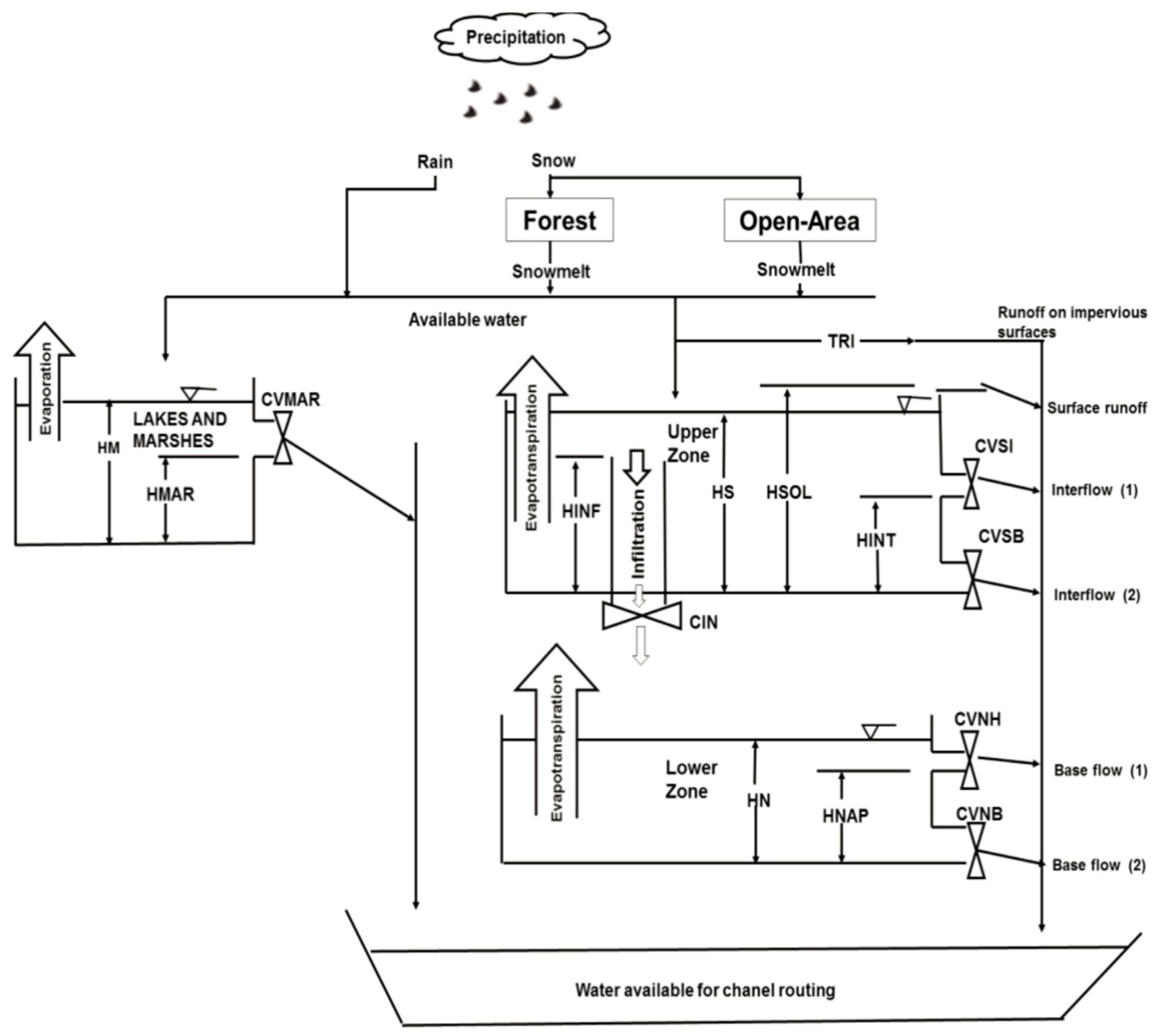
2.2. CEQUEAU Model
- Short wave radiation (measured);
- Long wave incoming and backscattered radiation (calculated using the Stefan–Boltzmann equation; [23]);
- Evapotranspiration (latent heat; calculated as a function of the difference between saturated vapor pressure and water vapor pressure in the air; [23]);
- Convection (sensible heat; estimated from an empirical equation based on the Bowen Ratio; [23]);
- Upstream and downstream advection;
- Local heat advection (from runoff, interflow and groundwater inputs).
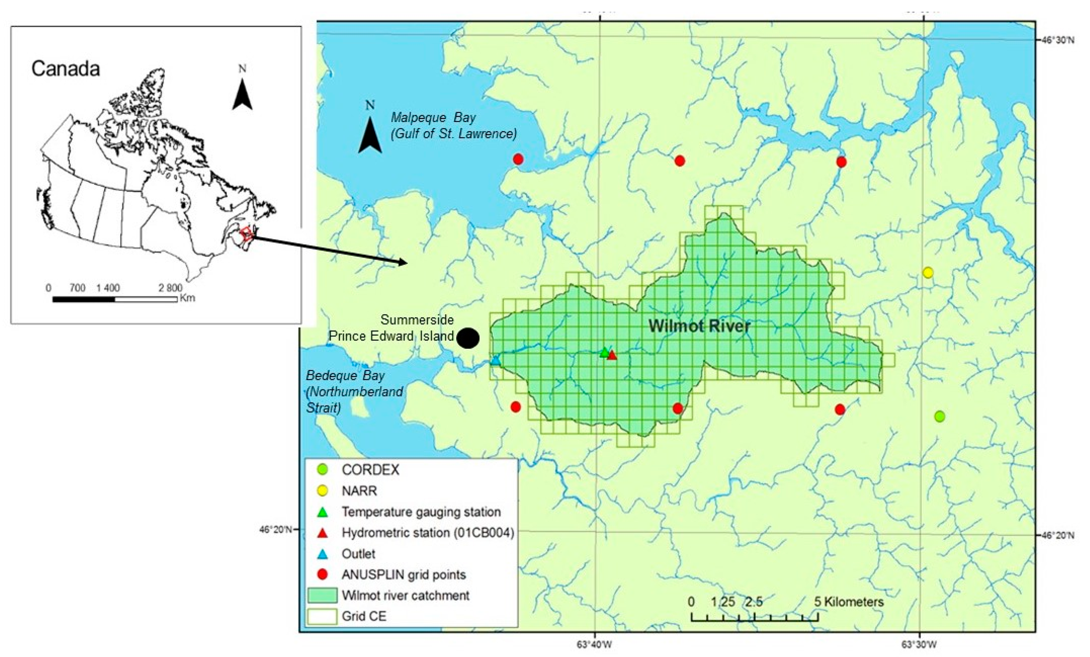
2.3. Study Site, Model Implementation and Calibration
2.4. Climate Change Scenarios
3. Results
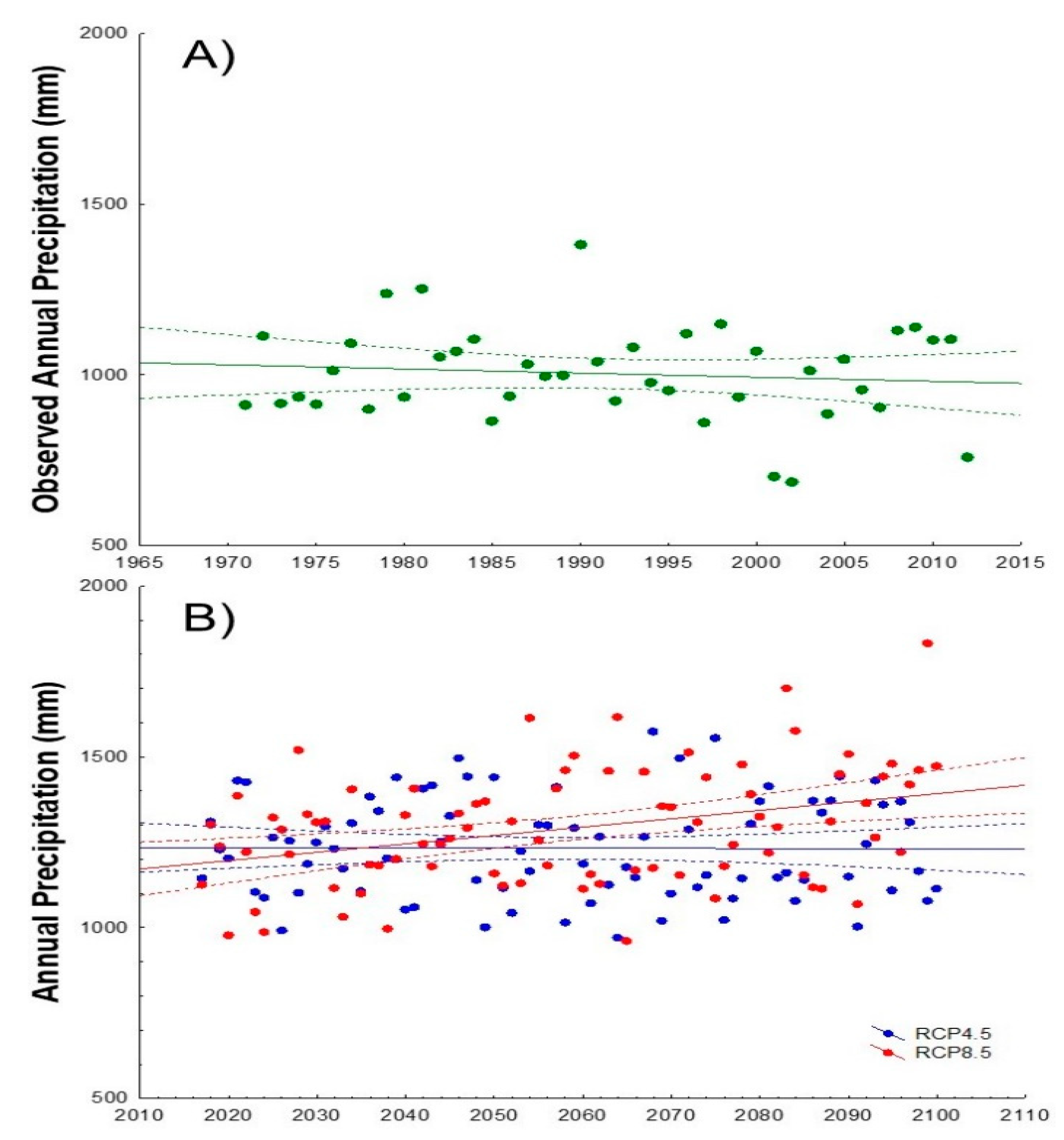
3.1. Climate Change Precipitation Scenarios
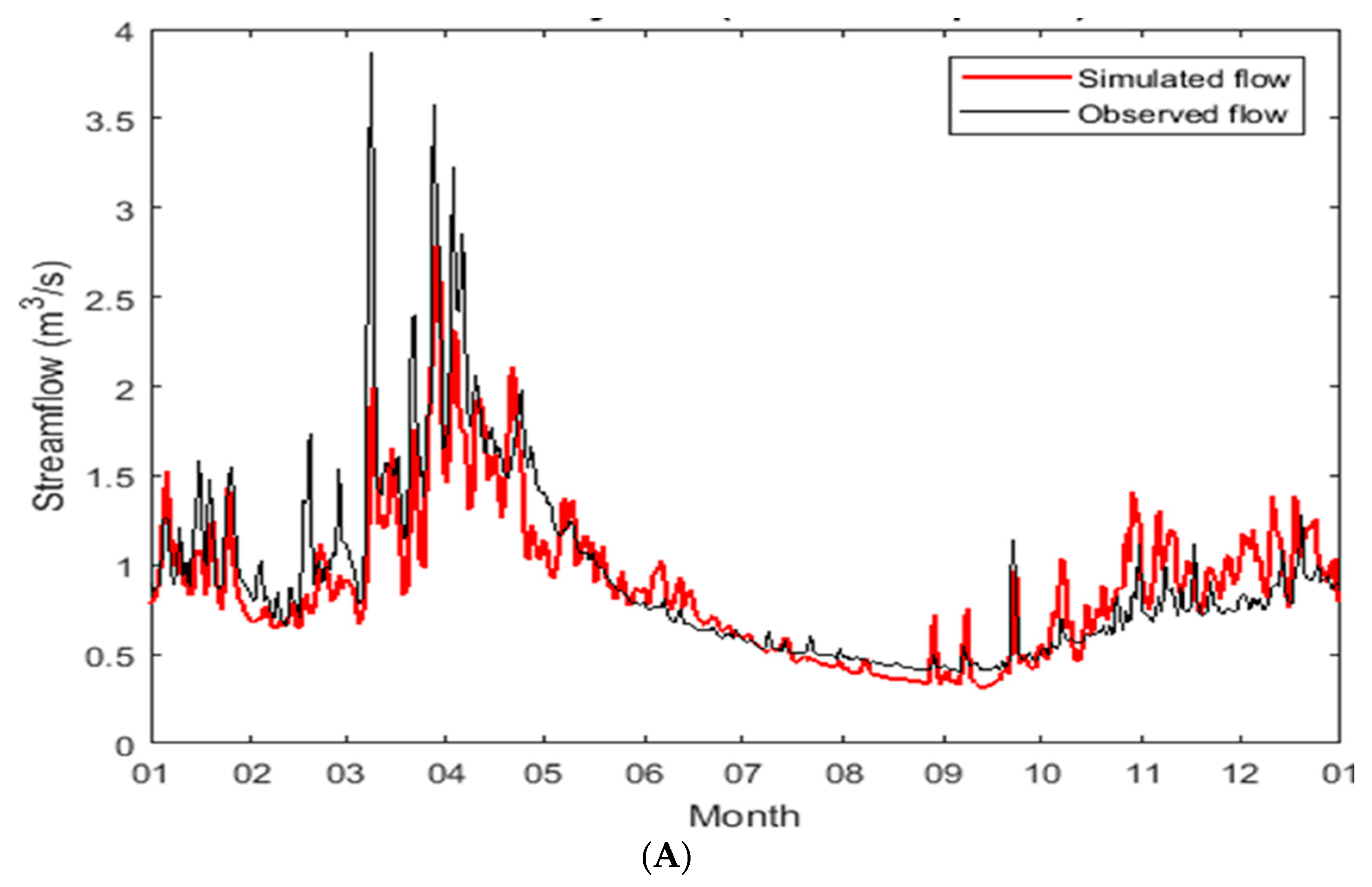
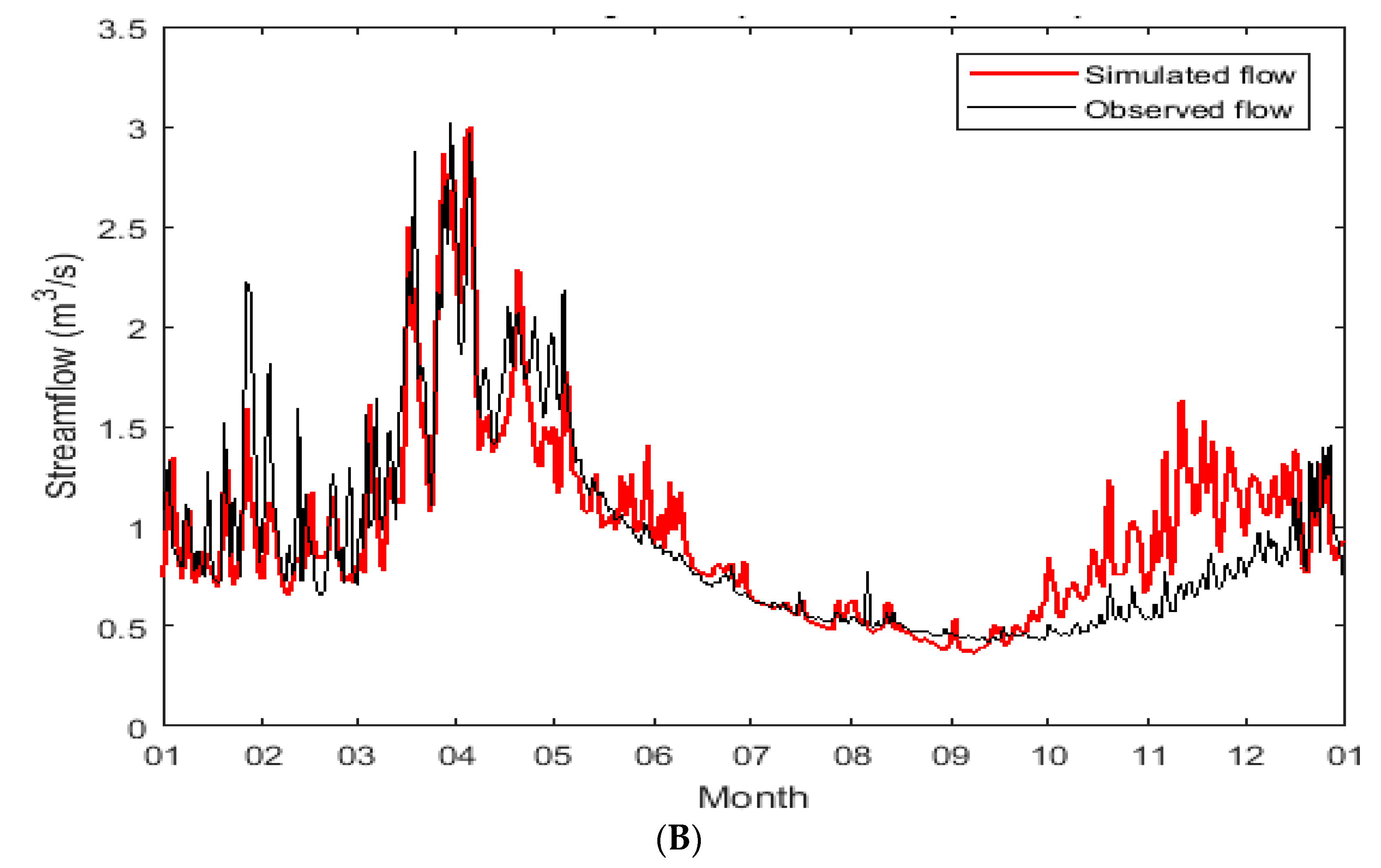
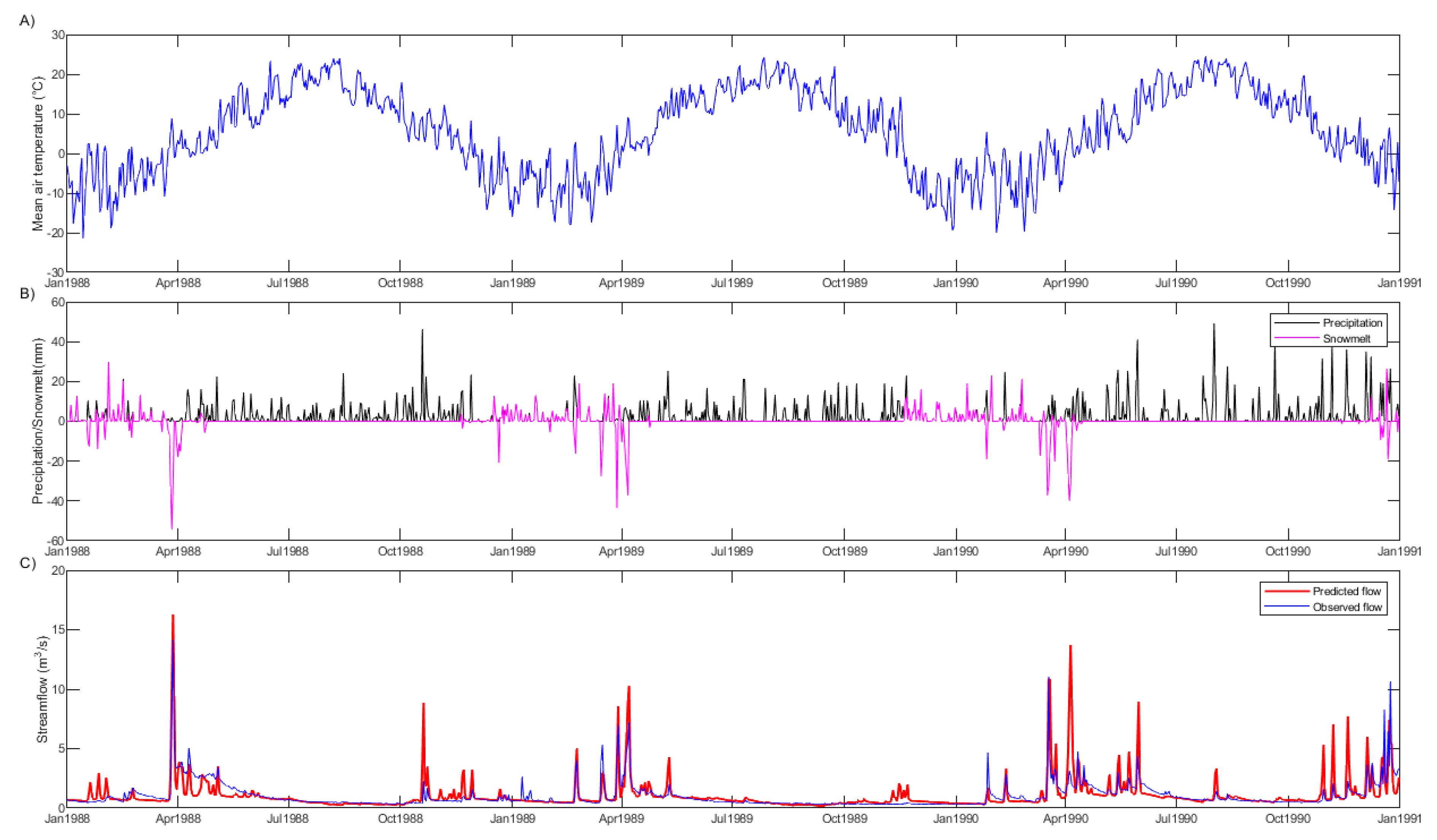
3.2. Flow Model Calibration and Validation
3.3. Temperature Model Calibration and Validation
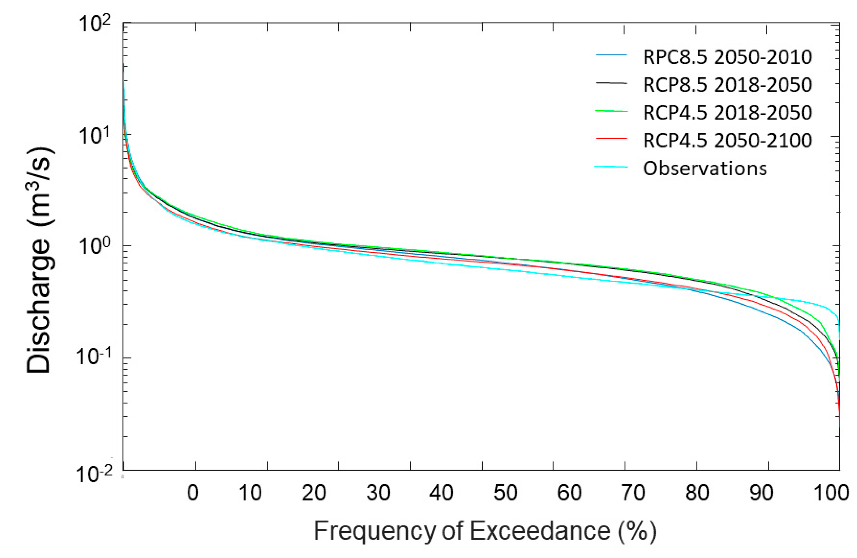
3.4. Climate Change Flow Scenarios
4. Discussions and Conclusions
Author Contributions
Funding
Institutional Review Board Statement
Informed Consent Statement
Data Availability Statement
Acknowledgments
Conflicts of Interest
Nomenclature
| Q | mm | Total runoff for a whole square |
| P | mm | Rain or snowmelt for a whole square |
| ETP | mm | Evapotranspiration for a whole square |
| HU | mm | Water accumulated in the upper reservoir for a whole square |
| HL | mm | Water accumulated in the lower reservoir for a whole square |
| CIN | - | Percolation coefficient from the upper-zone to the lower-zone |
| CVMAR | Lakes and marshes drainage coefficient | |
| CVNB | Lower-zone lower drainage coefficient | |
| CVNH | Lower-zone upper drainage coefficient | |
| CVSB | Upper-zone lower drainage coefficient | |
| CVSI | - | Upper-zone intermediate drainage coefficient |
| HINF | mm | Percolation threshold from the upper to the lower-zone |
| HINT | mm | Upper-zone intermediate drainage threshold |
| HM | mm | Lakes and Marshes reservoir water level |
| HMAR | mm | Lakes and Marshes drainage threshold |
| HN | mm | Lower-zone reservoir water level |
| HNAP | mm | Lower-zone upper threshold |
| HS | mm | Upper-zone runoff reservoir water level |
| HSOL | mm | Upper-zone runoff threshold |
| TRI | % | Percentage of impervious area in the basin |
| XKT | - | Routing coefficient |
| EXXKT | Routing coefficient fitting parameter | |
| RMA3 | km2 | Area of the basin upstream of the partial square |
| Sl | km2 | Area of the total surface water upstream of the partial square |
| Slac | km2 | Area of surface water on the partial square |
| CEKM2 | Area of the whole square | |
| Tw | °C | Water temperature |
| H | MJ | Total enthalpy of the thermodynamic system |
| V | m3 | Volume of water |
| C | MJ/m3/°C | Heat capacity of water (4.187) |
References
- Arthington, A.H.; Bhaduri, A.; Bunn, S.E.; Jackson, S.E.; Tharme, R.E.; Tickner, D.; Young, B.; Acreman, M.; Baker, N.; Capon, S.; et al. The Brisbane Declaration and global action agenda on environmental flows (2018). Front. Environ. Sci. 2018, 6, 45. [Google Scholar] [CrossRef] [Green Version]
- Tennant, D.L. Instream Flow Regimens for Fish, Wildlife, Recreation and Related Environmental Resources. Fisheries 1976, 1, 6–10. [Google Scholar] [CrossRef]
- Theodoropoulos, C.; Vourka, A.; Skoulikidis, N.; Rutschmann, P.; Stamou, A. Evaluating the performance of habitat models for predicting the environmental flow requirements of benthic macroinvertebrates. J. Ecohydraulics 2018, 3, 30–44. [Google Scholar] [CrossRef]
- King, J. Instream Flow Assessments for Regulated Rivers in South Africa Using the Building Block Methodology. Aquat. Ecosyst. Health Manag. 1998, 1, 109–124. [Google Scholar] [CrossRef]
- Poff, N.; Leroy, B.D.; Arthington, A.H.; Bunn, S.E.; Naiman, R.J.; Kendy, E.; Acreman, M.; Apse, C.; Bledsoe, B.P.; Freeman, M.C.; et al. The Ecological Limits of Hydrologic Alteration (ELOHA): A New Framework for Developing Regional Environmental Flow Standards: Ecological Limits of Hydrologic Alteration. Freshw. Biol. 2010, 55, 147–170. [Google Scholar] [CrossRef] [Green Version]
- Pahl-Wostl, C.; Arthington, A.; Bogardi, J.; Bunn, S.E.; Hoff, H.; Lebel, L.; Nikitina, E.; Palmer, M.; Poff, L.N.; Richards, K.; et al. Environmental flows and water governance: Managing sustainable water uses. Curr. Opin. Environ. Sustain. 2013, 5, 341–351. [Google Scholar] [CrossRef]
- Jowett, I.G. Instream flow methods: A comparison of approaches. Regul. Rivers Res. Manag. 1997, 13, 115–127. [Google Scholar] [CrossRef]
- Dunbar, M.J.; Acreman, M.; Kirk, S. Environmental Flow Setting in England and Wales: Strategies for Manag-ing Abstraction in Catchments. Water Environ. J. 2004, 18, 4–10. [Google Scholar] [CrossRef]
- Caissie, D.; Eljabi, N. Hydrologically Based Environmental Flow Methods Applied to Rivers in the Maritime Provinces (Canada). River Res. Appl. 2015, 31, 651–662. [Google Scholar] [CrossRef]
- El-Jabi, N.; Caissie, D. Characterization of natural and environmental flows in New Brunswick, Canada. River Res. Appl. 2018, 35, 14–24. [Google Scholar] [CrossRef] [Green Version]
- Olden, J.D.; Naiman, R.J. Incorporating Thermal Regimes into Environmental Flows Assessments: Modifying Dam Operations to Restore Freshwater Ecosystem Integrity: Incorporating Thermal Regimes in Environmental Flows Assessments. Freshw. Biol. 2010, 55, 86–107. [Google Scholar] [CrossRef]
- Essaid, H.I.; Caldwell, R.R. Evaluating the impact of irrigation on surface water—Groundwater interaction and stream temperature in an agricultural watershed. Sci. Total Environ. 2017, 599–600, 581–596. [Google Scholar] [CrossRef]
- Michie, L.E.; Thiem, J.D.; Boys, C.A.; Mitrovic, S.M. Erratum to: The effects of cold shock on freshwater fish larvae and early-stage juveniles: Implications for river management. Conserv. Physiol. 2020, 8, coaa106. [Google Scholar] [CrossRef]
- Daigle, A.; Jeong, D.I.; Lapointe, M.F. Climate change and resilience of tributary thermal refugia for salmonids in eastern Canadian rivers. Hydrol. Sci. J. 2015, 60, 1044–1063. [Google Scholar] [CrossRef]
- Jeong, D.I.; Daigle, A.; St-Hilaire, A. Development of a stochastic water temperature model and projection of future water temperature and extreme events in the ouelle river basin in québec, canada. River Res. Appl. 2012, 29, 805–821. [Google Scholar] [CrossRef]
- Van Vliet, M.T.; Franssen, W.H.; Yearsley, J.R.; Ludwig, F.; Haddeland, I.; Lettenmaier, D.P.; Kabat, P. Global river discharge and water temperature under climate change. Glob. Environ. Chang. 2013, 23, 450–464. [Google Scholar] [CrossRef]
- Morin, G.; Sochanski, W.; Paquet, P. Le Modèle de Simulation de Quantité Cequeau-Onu, Manuel de Référence; INRS-Eau: Québec City, QC, Canada, 1998. [Google Scholar]
- St-Hilaire, A.; Boucher, M.-A.; Chebana, F.; Ouellet-Proulx, S.; Zhou, Q.X.; Larabi, S.; Dugdale, S.; Latraverse, M. Breathing new life into an old model: The CEQUEAU tool for flow and temperature simulations and forecasting. In Proceedings of the 22nd Canadian Hydrotechnical Conference, Montreal, QC, Canada, 29 April–2 May 2015; p. 7. [Google Scholar]
- Kwak, J.; St-Hilaire, A.; Chebana, F.; Kim, G. Summer Season Water Temperature Modeling under the Climate Change: Case Study for Fourchue River, Quebec, Canada. Water 2017, 9, 346. [Google Scholar] [CrossRef] [Green Version]
- Dugdale, S.J.; Curry, R.A.; St-Hilaire, A.; Andrews, S.N. Impact of Future Climate Change on Water Temperature and Thermal Habitat for Keystone Fishes in the Lower Saint John River, Canada. Water Resour. Manag. 2018, 32, 4853–4878. [Google Scholar] [CrossRef]
- Mann, H.B. Nonparametric tests against trend. Econometrica 1945, 13, 245–259. [Google Scholar] [CrossRef]
- Clarke, K.R.; Gorley, R.N. Primer V6: User Manual/Tutorial; PRIMER-E: Plymouth, UK, 2006. [Google Scholar]
- Morin, G.; Couillard, D. Predicting River Temperatures with a Hydrological Model; Encyclopedia of Fluid Mechanics, 10; Gulf Publishing Compagny: Hudson, TX, USA, 1990; pp. 171–209. [Google Scholar]
- St-Hilaire, A.; Morin, G.; ElL-Jabi, N.; Caissie, D.D. Water temperature modelling in a small forested stream: Implication of forest canopy and ground temperature. Can. J. Civ. Eng. 2000, 27, 1095–1108. [Google Scholar] [CrossRef]
- Larabi, S.; St-Hilaire, A.; Chebana, F.; Latraverse, M. Using Functional Data Analysis to Calibrate and Evaluate Hydrological Model Performance. J. Hydrol. Eng. 2018, 23, 04018026. [Google Scholar] [CrossRef]
- Hutchinson, M.F.; Mckenney, D.W.; Lawrence, K.; Pedlar, J.H.; Hopkinson, R.F.; Milewska, E.; Papadopol, P. Development and Testing of Canada-Wide Interpolated Spatial Models of Daily Minimum-Maximum Temperature and Precipitation for 1961–2003. J. Appl. Meteorol. Climatol. 2009, 48, 725–741. [Google Scholar] [CrossRef]
- Frei, C.; Schöll, R.; Fukutome, S.; Schmidli, J.; Vidale, P.L. Future change of precipitation extremes in Europe: Intercom-parison of scenarios from regional climate models. J. Geophys. Res. 2006, 111, D6. [Google Scholar] [CrossRef] [Green Version]
- Lafon, T.; Dadson, S.; Buys, G.; Prudhomme, C. Bias correction of daily precipitation simulated by a regional climate model: A comparison of methods. Int. J. Clim. 2013, 33, 1367–1381. [Google Scholar] [CrossRef] [Green Version]
- Gutowski, W.J., Jr.; Giorgi, F.; Timbal, B.; Frigon, A.; Jacob, D.; Kang, H.-S.; Raghavan, K.; Lee, B.; Lennard, C.; Nikulin, G.; et al. WCRP COordinated Regional Downscaling EXperiment (CORDEX): A diagnostic MIP for CMIP6. Geosci. Model. Dev. 2016, 9, 4087–4095. [Google Scholar] [CrossRef] [Green Version]
- Böhnisch, A.; Ludwig, R.; LeDuc, M. Using a nested single-model large ensemble to assess the internal variability of the North Atlantic Oscillation and its climatic implications for central Europe. Earth Syst. Dyn. 2020, 11, 617–640. [Google Scholar] [CrossRef]
- Birkel, S.D.; Mayewski, P.A.; Maasch, K.A.; Kurbatov, A.V.; Lyon, B. Evidence for a volcanic underpinning of the Atlantic multidecadal oscillation. NPJ Clim. Atmos. Sci. 2018, 1, 24. [Google Scholar] [CrossRef] [Green Version]
- Kynsh, K.; DGiberson, J.; van den Heuvel, M.R. The influence of agricultural land-use on plant and macroin-vertebrate communities in springs in Eastern Prince Edward Island, Canada. Limnol. Oceanogr. 2016, 61, 518–530. [Google Scholar]
- Brungs, W.A.; Jones, B.R. Temperature Criteria for Freshwater Fish: Protocol and Procedures; US Environmental Protection Agency Report EPA-600/3-77-061; USEP: Duluth, MN, USA, 1977; p. 130. [Google Scholar]
- Von Trentini, F.; Leduc, M.; Ludwig, R. Assessing natural variability in RCM signals: Comparison of a multimodel EURO-CORDEX ensemble with a 50-member single model large ensemble. Clim. Dyn. 2019, 53, 1963–1979. [Google Scholar] [CrossRef] [Green Version]


| Calibration Sample (1992–2012) | Validation Sample (1972–1991) | |
|---|---|---|
| KGE (%) | 57.63 | 64.98 |
| Bias (m3/s) | −0.041 | 0.031 |
| RMSE (m3/s) | 1.038 | 0.973 |
| Validation Sample (5-Fold Cross-Validation) | Validation Sample (Average Parameters) | |||||
|---|---|---|---|---|---|---|
| 2013 | 2014 | 2015 | 2016 | 2017 | 2013–2017 | |
| KGE (%) | 79.66 | 86.56 | 93.00 | 89.33 | 95.16 | 93.54 |
| Bias (°C) | 0.00 | 0.71 | 0.40 | 0.11 | −0.34 | 0.20 |
| RMSE (°C) | 1.37 | 1.35 | 1.16 | 0.96 | 1.03 | 1.08 |
| Observations | RCP 4.5 2018–2050 | RCP 4.5 2051–2100 | RCP 8.5 2018–2050 | RCP 8.5 2051–2100 | |
|---|---|---|---|---|---|
| Q50 (m3/s) | 0.45 | 0.49 | 0.59 | 0.57 | 0.48 |
| Q95 (m3/s) | 0.33 | 0.17 | 0.16 | 0.18 | 0.12 |
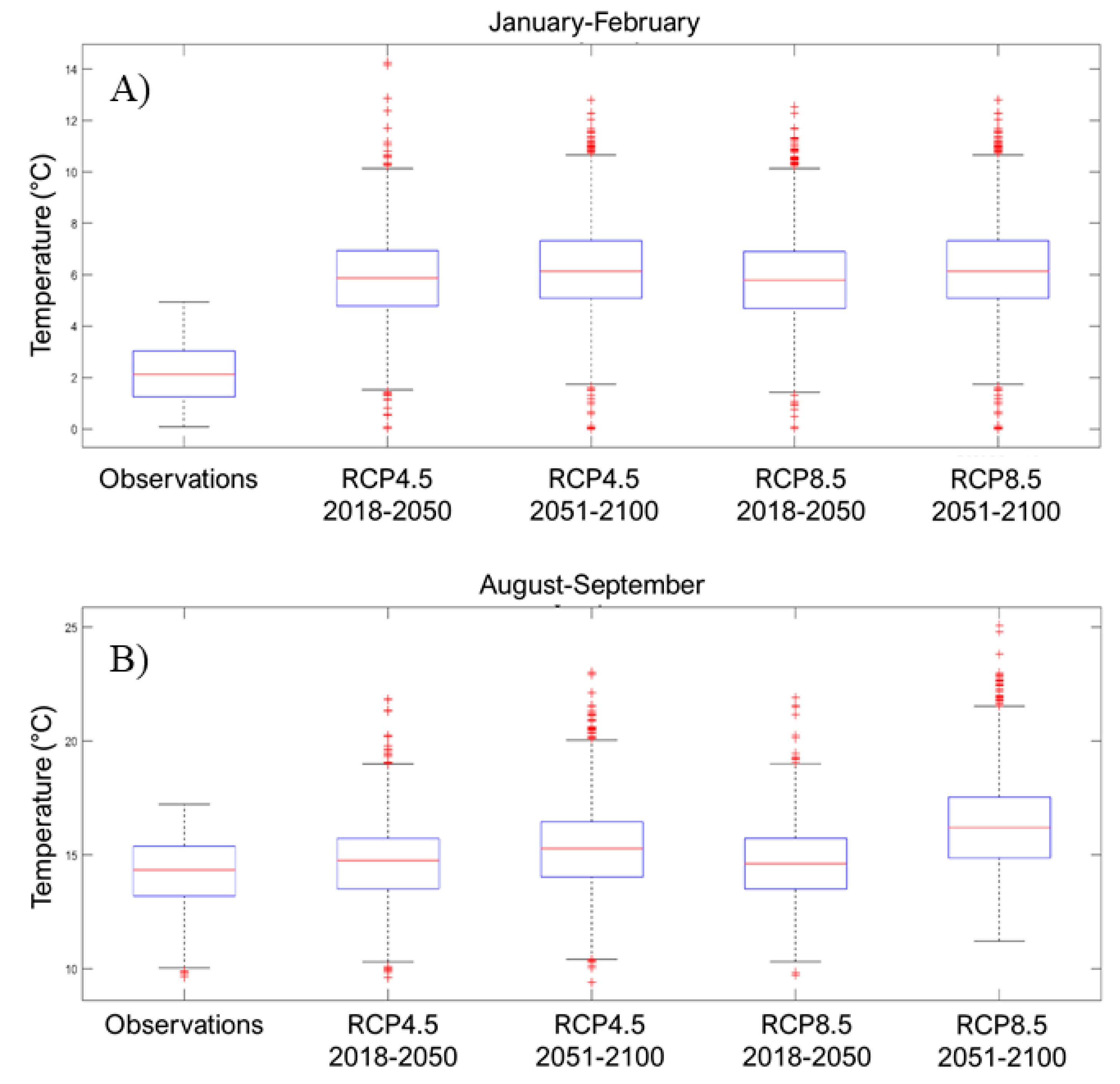
| Slope Parameter (°C/Decade) | January | February | August | September |
|---|---|---|---|---|
| RCP 4.5 | ||||
| Minimum | 0.009 (0.169) | 0.007 (0.085) | 0.008 (0.078) | -0.002 (0.904) |
| Mean | 0.005 (0.163) | 0.007 (0.068) | 0.011 (0.001) | 0.0002 (0.055) |
| Maximum | 0.009 (0.074) | 0.007 (0.067) | 0.013 (0.020) | 0.002 (0.984) |
| RCP 8.5 | ||||
| Minimum | 0.25 (<0.001) | 0.32 (<0.001) | 0.29 (<0.001) | 0.28 (<0.001) |
| Mean | 0.24 (<0.001) | 0.29 (<0.001) | 0.35 (<0.001) | 0.31 (<0.001) |
| Maximum | 0.31 (<0.001) | 0.29 (<0.001) | 0.40 (<0.001) | 0.32 (<0.001) |
Publisher’s Note: MDPI stays neutral with regard to jurisdictional claims in published maps and institutional affiliations. |
© 2021 by the authors. Licensee MDPI, Basel, Switzerland. This article is an open access article distributed under the terms and conditions of the Creative Commons Attribution (CC BY) license (https://creativecommons.org/licenses/by/4.0/).
Share and Cite
Charron, C.; St-Hilaire, A.; Ouarda, T.B.M.J.; van den Heuvel, M.R. Water Temperature and Hydrological Modelling in the Context of Environmental Flows and Future Climate Change: Case Study of the Wilmot River (Canada). Water 2021, 13, 2101. https://doi.org/10.3390/w13152101
Charron C, St-Hilaire A, Ouarda TBMJ, van den Heuvel MR. Water Temperature and Hydrological Modelling in the Context of Environmental Flows and Future Climate Change: Case Study of the Wilmot River (Canada). Water. 2021; 13(15):2101. https://doi.org/10.3390/w13152101
Chicago/Turabian StyleCharron, Christian, André St-Hilaire, Taha B.M.J. Ouarda, and Michael R. van den Heuvel. 2021. "Water Temperature and Hydrological Modelling in the Context of Environmental Flows and Future Climate Change: Case Study of the Wilmot River (Canada)" Water 13, no. 15: 2101. https://doi.org/10.3390/w13152101