
Parametric Analysis for Underwater Flapping Foil Propulsor


1
School of Naval Architecture and Ocean Engineering, Harbin Institute of Technology, Weihai 264209, China
2
Department of Naval Architecture, Ocean and Marine Engineering, Strathclyde University, Glasgow G4 0LZ, UK
*
Author to whom correspondence should be addressed.
Water 2021, 13(15), 2103; https://doi.org/10.3390/w13152103
Submission received: 28 June 2021
/
Revised: 27 July 2021
/
Accepted: 29 July 2021
/
Published: 31 July 2021
(This article belongs to the Section Hydraulics and Hydrodynamics)
Abstract
:This paper researched into the harmonic and anharmonic underwater flapping foil propulsion systems to improve the efficiency of these bioinspired propulsors. The angle of attack, the pitching angle, the heaving amplitude, and the phase difference are parametrically investigated in this paper. A rigid two-dimensional NACA (National Advisory Committee for Aeronautics) 0012 airfoil is modeled with the aid of a commercial computational fluid dynamics software, FINE™/Marine. Unsteady Reynolds Average Navier-Stokes (URANS) equation is solved together with dynamic mesh to simulate the foil motion. The investigation first verifies the reliability of the developed modeling method against the benchmark data. Then, the systematic investigation is conducted and identifies that the heaving amplitude is most influential factor for the propulsion efficiency. Secondly, phase difference also has a significant influence on efficiency, but this effect is related to the reference working condition, which needs further study. Then, the pitching amplitude has little effect on the maximum efficiency value of flapping foil, while it will affect its optimal speed range. When the heaving amplitude ratio reaches 3 and the corresponding maximum angle of attack is about 9°, the maximum efficiency can reach 87%. The effect of anharmonic motion on the efficiency is very small and varies with the St number, but in summary, it can maintain the peak efficiency over a wider range of operations. In addition, the force and flow field characteristics of different efficiency points are compared and analyzed to distinguish their corresponding relationship with the propulsion efficiency.
1. Introduction
Natural swimmers such as fish and aquatic mammals have beautifully evolved to be able to utilize the physical principles of unsteady hydrodynamics to achieve both high maneuverability and high propulsive efficiency [1]. The basic source of locomotion and maneuvering is from the flapping foil, which can generally perform simultaneous translational and rotational motions in two or more degrees of freedom. And during flapping, the vortices can be rolled up into the wake region forming inverse von-Karman vortex streets to assist the propulsion [2]. It is noteworthy that the efficiency of flapping foil can reach 80% as evidenced in the experimental tests [3,4,5,6]. In contrast, most of the conventional propellers which existing waterborne vehicles are relying on, presents lower propulsive efficiency, lower maneuverability, and higher radiated noise level. The application of flapping foil propulsion could remedy the above disadvantages [7,8,9,10]. In addition, the flapping foil propulsion is naturally equivalent to a variable-pitch propulsion system [5], which provides a wide range of operating profiles for both surface and underwater vehicles. Therefore, growing attention has been devoted to the research of flapping foil application for waterborne vehicles, including natural observation, theoretical analysis, experimental studies, and computational investigations.
High propulsion efficiency is one of the core characteristics of a flapping foil propeller. In order to explore the mechanism of high efficiency of flapping foil propeller, and achieve the optimal efficiency, a lot of research has been carried out.
The initial research mainly focused on the efficiency measurement of conventional simple harmonic flapping foil and the analysis of the influence of foil parameters on efficiency. Anderson [3] measured the thrust coefficients and the efficiency of a flapping foil at different Strouhal numbers (St). The efficiency was measured to be peaked at 87%. Read [11] and Schoveiler [4] carried out similar work afterward. The highest efficiency in their experiments was 70% and 73%, respectively. However, Schoveiler’s theoretical analysis showed that the highest efficiency could reach 81%. By using a potential based 3D boundary element method (BEM), Politis and Tsarsitalidis [12] presented an atlas of wake vortex development for various foil and loading conditions elucidating the mechanism of thrust producing vortex. The same method is used by Floc’h et al. [5] for further research. They studied the effect of different St numbers, different heave amplitudes and different flap angle amplitudes on the efficiency, and the highest efficiency was achieved 84.5%. By solving the vortex equations, Guglielmini et al. [13] determined the dynamics of the vortex structures generated by a foil. The effect on efficiency caused by the pitch amplitude, the heave amplitude and the phase angle were also analyzed to identify the optimal parameter settings to maximize the propulsive efficiency, and they achieved is about 47.5% maximum efficiency. In 2017, Floryan et al. [14] tried to correlate the efficiency to the St number and the reduced frequency in water tunnel experiments but its maximum efficiency only reached about 27%. In conclusion, although the research on simple harmonic two-dimensional oscillation foil has a long history, its physical mechanism is not clear in some aspects, and some scholars continue to study this. At the same time, many of the above studies on foil mechanism parameters are not carried out near the optimal efficiency point, that is, the research data on the influence of foil parameters near the theory’s highest efficiency point (80%) need to be further supplemented and improved.
Many scholars have also been concerned with research on the propulsion performance of flapping foil, the effects of pure pitch motion, pure heave motion and anharmonic motion trajectory on efficiency have also been concerned by many scholars. In 2009, Schnipper [15] presented a detailed observation on the vortex structure of a symmetric foil performing pitching oscillations. Similiarly, Andersen et al. [16] researched into a heaving foil that demonstrated to be easier to produce thrust than a pitching foil. And he pinpointed the essential features of this vortex structure and the phase diagram of wake corresponding to different parameters. The effects of Reynolds number, phase angle, and pivot location on the self-propulsion performance in three different operating conditions were numerically studied by Lin in 2019 [17]. They achieved 70% maximum efficiency. On the other hand, read et al. [11] noted that for high St numbers, the thrust coefficient deteriorates rapidly because the induced angle of attack (AoA) ceases to be harmonic. Building upon the method employed by Read et al., Hover et al. [18] directly compared the performance obtained with four specific AoA profiles in the experiment, including: (i) simple harmonic motion in both heave and pitch motion, (ii) a square wave, (iii) a symmetric sawtooth wave, and (iv) a cosine function. They found that explicit control of the AoA in flapping foil propulsion can broadly increase thrust and efficiency, compared to a baseline case in which the heave and pitch motions are sinusoidal. And their work was numerically extended by Xiao and Liao [19], by controlling the anharmonic motion trajectory, the efficiency is increased to 80%. Subsequently, Berman and Wang [20], Xiao [21], Xie [22] and Lu et al. [23,24] numerically investigated the propulsive performance and energy extraction performance of the flapping foil with nonsinusoidal oscillation. They found that better performance could be obtained with the imposed modification on pitching motion. However, Amiralaei et al. [25] states the symmetric kinematics has a better aerodynamic performance. Chao et al. [26] numerically investigate the force generation and wake structures of a nonsinusoidal periodic pitching foil. These studies showed that nonsinusoidal motion has a noticeable effect on the foil’s propulsive performance, including the instantaneous force coefficients, the maximum time-mean thrust coefficients, and wake structures. However, most of the research focused on anharmonic pitching only foil or anharmonic heave only motion, and most of the parameter research is not carried out near the theory’s optimal efficiency point (80%) of the flapping foil. Therefore, a more comprehensive analysis on the anharmonic motion of a flapping foil with combined motion needs to be done.
As reviewed above, the most significant advantage of the flapping foil is its high efficiency, and it is generally acknowledged that the factors affecting the propulsion efficiency include St number, heaving amplitude, pitching amplitude, and phase angle. However, as discussed, although the research on two-dimensional oscillating foil has a long history, its physical mechanism is not clear in some aspects [10]. On the one hand, many of the above studies on foil mechanism parameters are completed under some specific working conditions, and the coverage of working condition parameters is not comprehensive, so it is difficult to obtain quantitative and universal laws. On the other hand, to the authors’ knowledge, most of the parameter research is not carried out near the theory optimal efficiency point (80%) of the foil, harmonic flapping foil propulsion still needs a more comprehensive parametric analysis especially near the maximum efficiency point, to conclude the theoretical maximum efficiency. Meanwhile, further research should be devoted to investigating anharmonic flapping foil propulsion and discuss whether the anharmonic motion is still helpful to improve the efficiency near the maximum propulsion efficiency. Therefore, in this paper, the two-dimensional viscous flow over the harmonically/anharmonically heaving and pitching foils is simulated by CFD method. The systematic and parametric analysis will be conducted to correlate the influencing factors to the propulsive efficiency. In addition, the access to the velocity, vorticity fields as functions of space and time, input power characteristics, and force characteristics, could allow us to identify the underlying thrust production mechanisms more easily.
2. Description and Definition of Flapping Foil Propulsion
2.1. Definition of Flapping Foil Motion
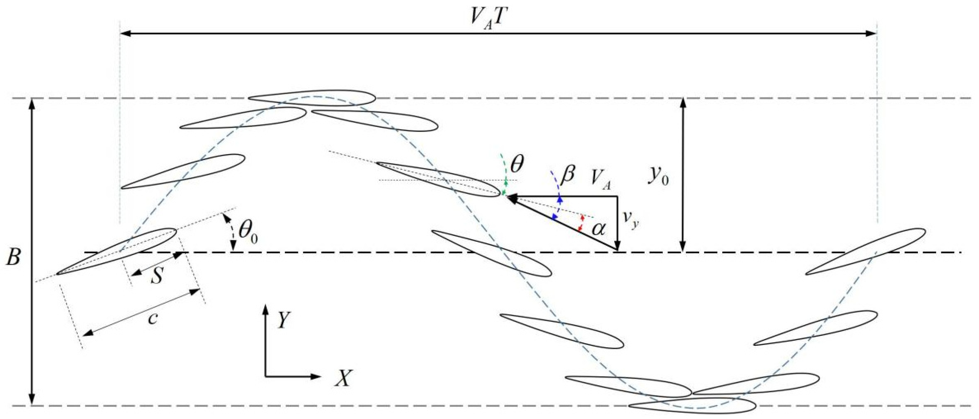
In this paper, a rigid two-dimensional NACA 0012 airfoil (developed by the National Aeronautical Advisory Committee (NACA), Moffett Field, CA, USA) is used, as shown in Figure 1. The flapping foil propulsor with a chord length, c, performs a combined pitch and heave motion with an advancing velocity VA (m/s), a period T (s) and a heave height B (m). The harmonic pitching and heaving motions can be described with the following classic definition [22,25], as shown in the Equations (1) and (2). The positive thrust and the forward direction are defined along the X direction and the heave direction is defined along the Y axis. The pitch motion is with regards to the Z axis. The pitching center is in a distance, S, from the leading-edge of the foil. The relationship between AoA α and the pitching angle θ is shown in Equation (3).
Heave motion:
Pitch motion:
where y0 is the heave amplitude, m; θ0 is the pitching amplitude, radian; f is the flapping frequency, Hz; φ is the phase angle difference between the heaving and pitching motions, radian; and t is the time, s; vy is the velocity component of the pivot center in the Y direction, m/s.
2.2. Nondimensional Propulsive Indicators
To study the flapping foil propulsion, some nondimensional numbers have been used in this paper. To nondimensionalize the flapping frequency, St Number is used, which is expressed as the following Equation (4).
For the convenience of comparing with marine propellers, Floc’h [5] introduced the advance coefficient, J as shown in the Equation (5), which is inherited in this paper.
The Reynolds number of the flapping foil can be expressed as follows in Equation (6).
where ν is the kinematic viscosity, m2/s.
According to Anderson et al. [3], the efficiency of the flapping motion is defined as the ratio of the average output and the average input power over a sufficient period of time. The input forces of the flapping foil consist of two parts: the heave force Fy, N, and the pitch torque Mz, Nm. The resulting hydrodynamic force is the thrust Fx in the forward direction. Neither the speed nor the force remains constant. Thus, the average input power is defined as Equation (7) with the average thrust in Equation (8).
where vy is the velocity component of the pivot center in the Y direction, and ωz is the angular velocity of the pivot center
The output power of the foil propeller is the product of the advancing velocity VA and the average thrust. Therefore, the efficiency of the flapping foil is defined as Equation (9).
Moreover, the thrust coefficient cT can be defined according to Anderson et al., 1998, as Equation (10).
where H is the length of wingspan, m, and ρ is the fluid density, kg/m3.
However, there are ongoing discussions about the reference area. With the introduction of heave motion, later in 2012 Floc’h [5] chose the swept area B × H instead of c × H the foil extension area as the reference area and followed the practice in the maritime industry of using KT as the thrust coefficient, as defined in Equation (11). This paper reckons the use of the swept area B × H as the reference area for flapping foils. However for the convenience of performing direct relevant comparison with the previous research, this paper will use both definitions. Hereby in this paper, KT is named as the propulsive thrust coefficient to be distinguished from the thrust coefficient cT.
2.3. Introducing the Anharmonic Motion
As mentioned in the previous introduction, some scholars have studied the oscillating foil with some anharmonic motion trajectory, and obtained the conclusion that the anharmonic trajectory could increase the efficiency and thrust of the flapping foil under some working conditions [16,17,26]. Based on this conclusion, the purpose of introducing the anharmonic motion trajectory in this paper is to further explore whether the anharmonic motion still helps to improve the propulsion efficiency under the condition close to the maximum propulsion efficiency.
To introduce the anharmonic motion, three possible types of anharmonic motions, e.g., anharmonic pitch only, anharmonic heave only, and combined, can be implemented. In this paper, the anharmonic motion is introduced by defining the motion function but maintaining the same heave amplitude throughout to perform a relative comparison with the harmonic flapping propulsion. According to the results of previous studies, the AoA is one of the determining parameters for efficiency, therefore of which the working duration at the optimum point needs to be maximized. This paper first introduces two types of anharmonic motions, the anharmonic pitch motion with the harmonic heave motion and the anharmonic heave motion with the anharmonic pitch motion. And it is found that it is not possible to use an anharmonic heave with anharmonic pitch motion, since this combination does not control the AoA to be optimum for the maximum duration. Therefore, it is not included in the investigation. The following two motions are described in detail in the following session.
2.3.1. Introducing the Anharmonic Pitch Motion
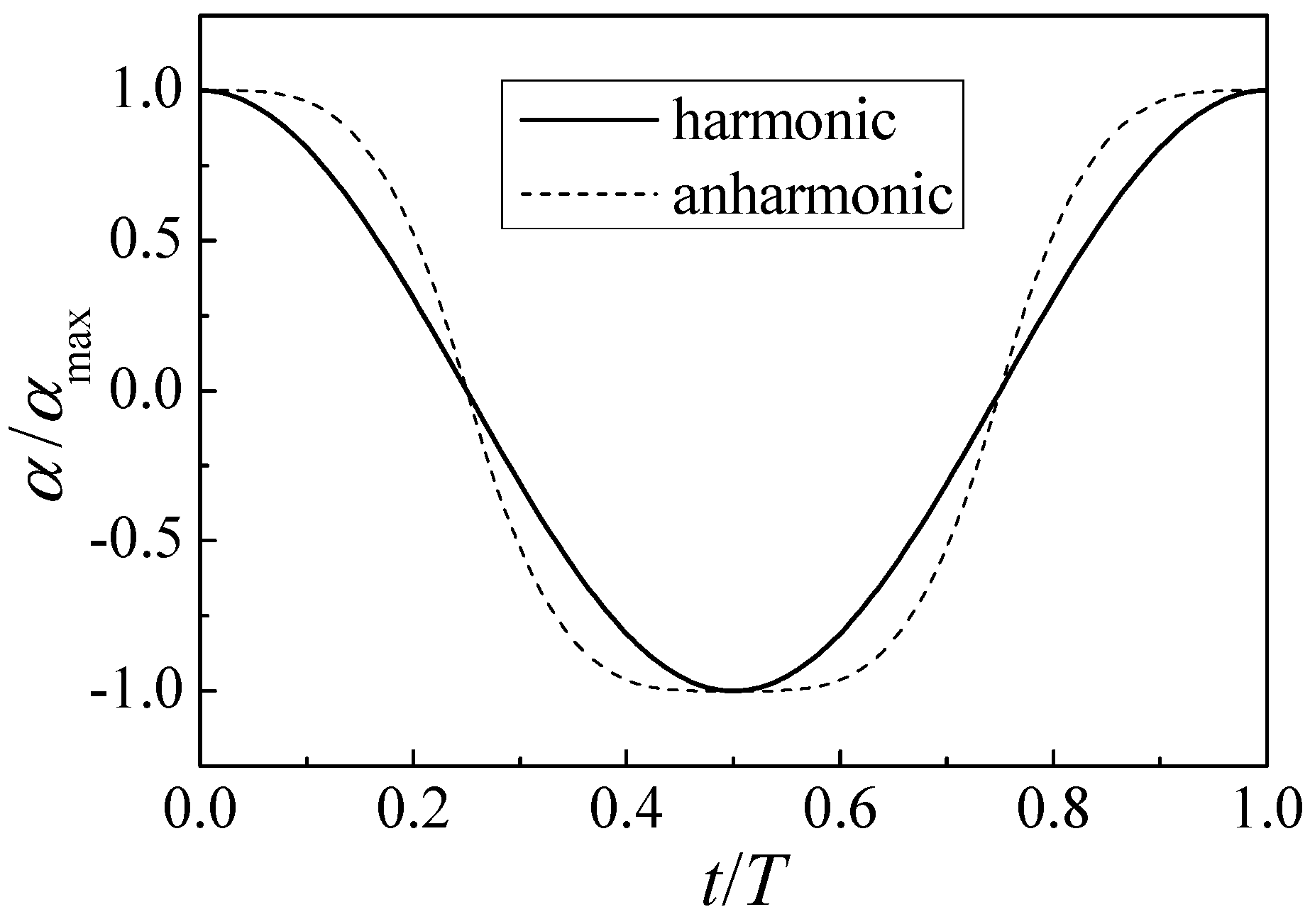
The aim of introducing an anharmonic motion for the foils is to maximize its working duration at the optimal AoA so that the forces and hence the power output can be maximized. To do this, a new periodic function gn(t) is introduced for AoA in the following Equation (12). It is developed to introduce a plumper periodic curve than the sine curve. Figure 2 shows the AoA curve comparisons between the g0(t) and g1(t).
where N is a set of positive integers, function F(x) is expressed as
When n is not an integer, its value can be obtained by linear interpolation, such as
Then, according to the relationship between AoA α and pitching angle θ, the pitching angle curve can be obtained from Equation (3).
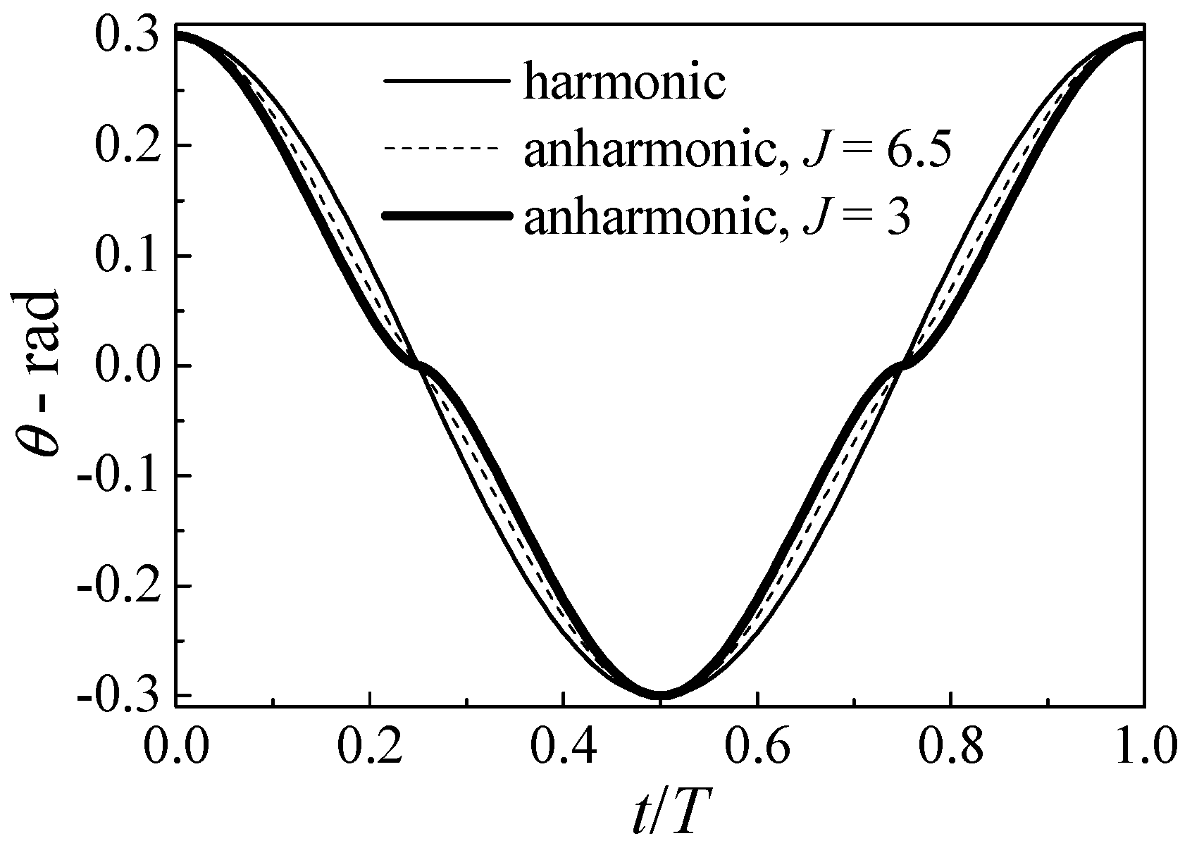
It can be seen from the Equation (3), when the foil heave motion is defined, the pitching angle θ is related to the AoA α and the St number. To maintain the same pitching amplitude θ0 for comparison, the AoA will vary with the St Number. Two St Numbers, 1/3 and 1/6.5, respectively, were chosen for the study, which correspond to the two cases of J = 3 and J = 6.5, presented in the Figure 3. The maximum pitching angle is kept constant and the AoA of the two conditions were defined using g1(t) function with maximum AoA equal to 0.50845 and 0.15022, respectively.
2.3.2. Anharmonic Heave and Pitch Motion Combined
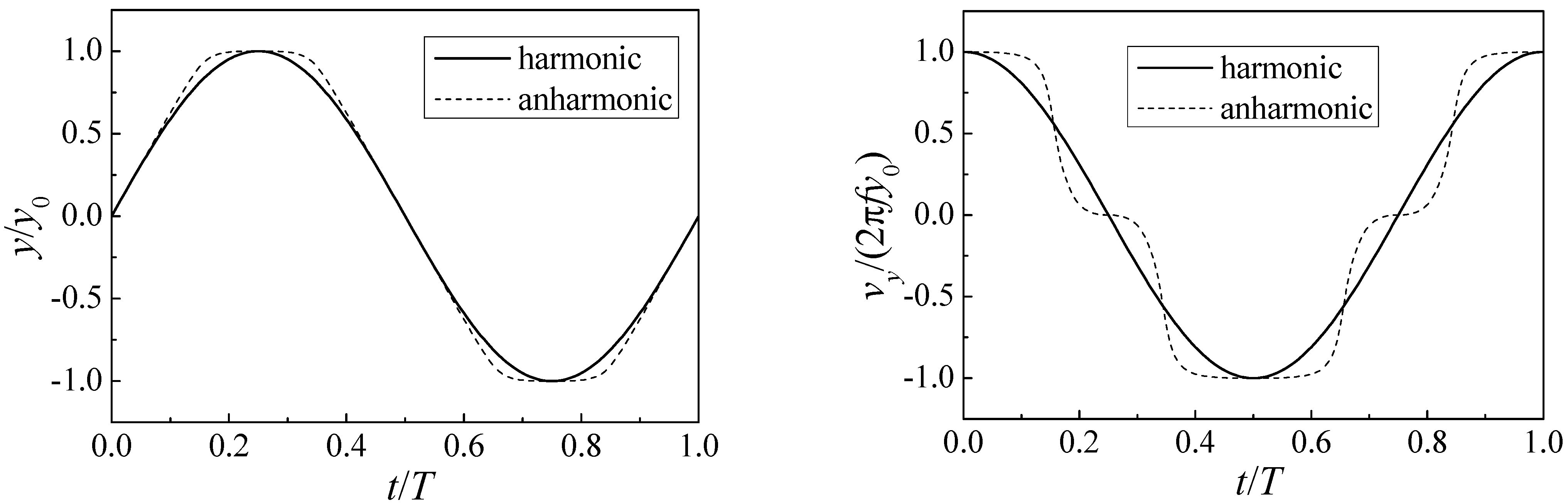
Similarly, when introducing the anharmonic heaving motion, a plumper velocity curve is expected. In the left figure of Figure 4, the heave displacement curve is close to the trapezoid curve and the velocity can be maximized at this condition as shown in the right figure of Figure 4.
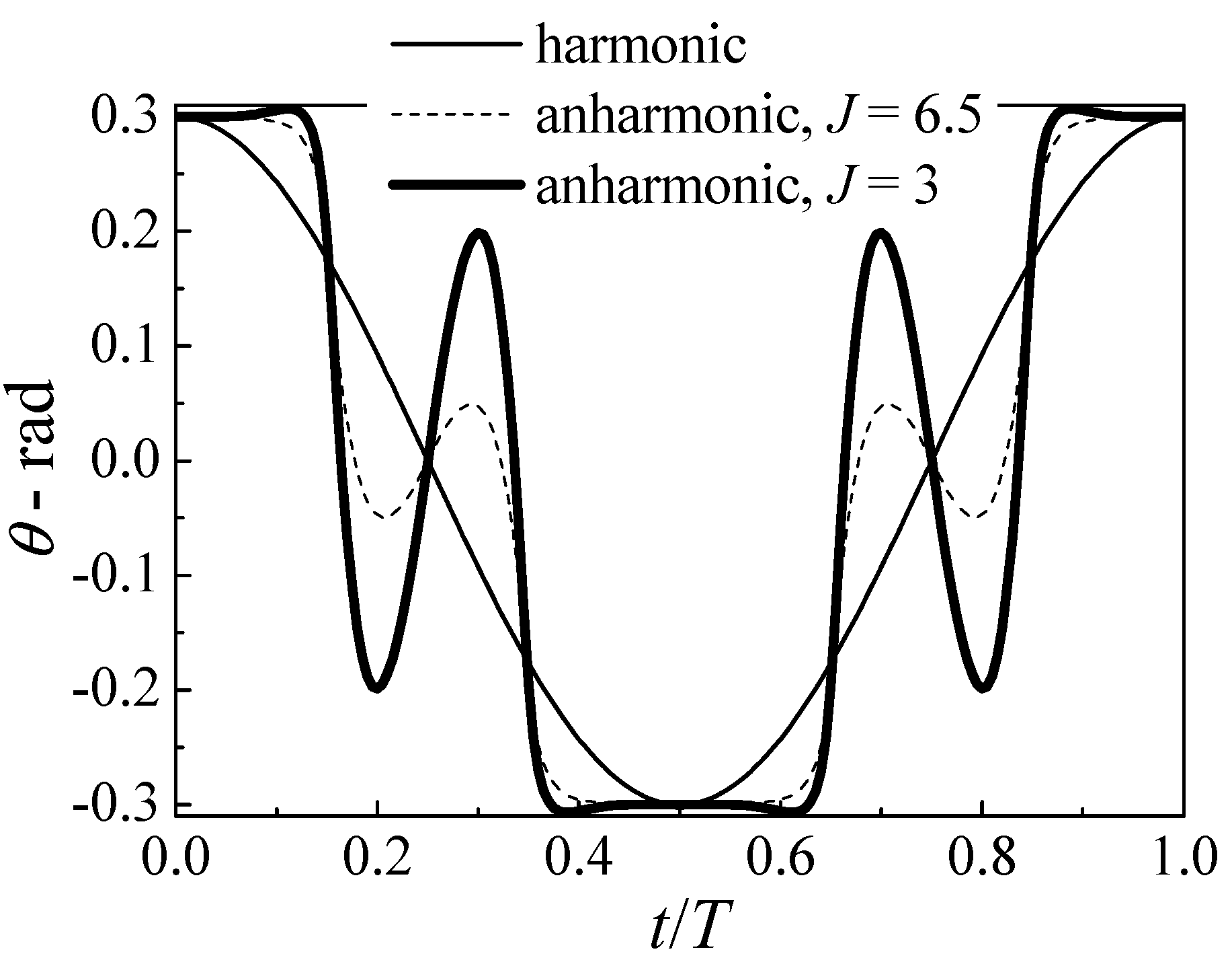
Subsequently, the curve of the attack angle is still constructed by g1(t) function. According to the relationship between the pitching angle, the attack angle, and the relative velocity angle, the curve of the pitching angle can be obtained. Because the design of the attack angle curve must take a certain St number as a reference. Here, the same two St numbers as before, 1/3 and 1/6.5, were chosen in this part, with the maximum pitching angle 0.3rad, to obtain two sets of pitching angle curves, as shown in Figure 5, denoted as anharmonic (J = 6.5) and anharmonic (J = 3), respectively. It can be seen from Figure 5 that there are some points of abrupt acceleration in the pitching angle curve, which means that the power in the rotation direction will increase. This is not conducive to improving efficiency. Therefore, the situation that both heaving motion and pitching motion are anharmonic is not analyzed further in this paper.
3. Computational Method and Validation
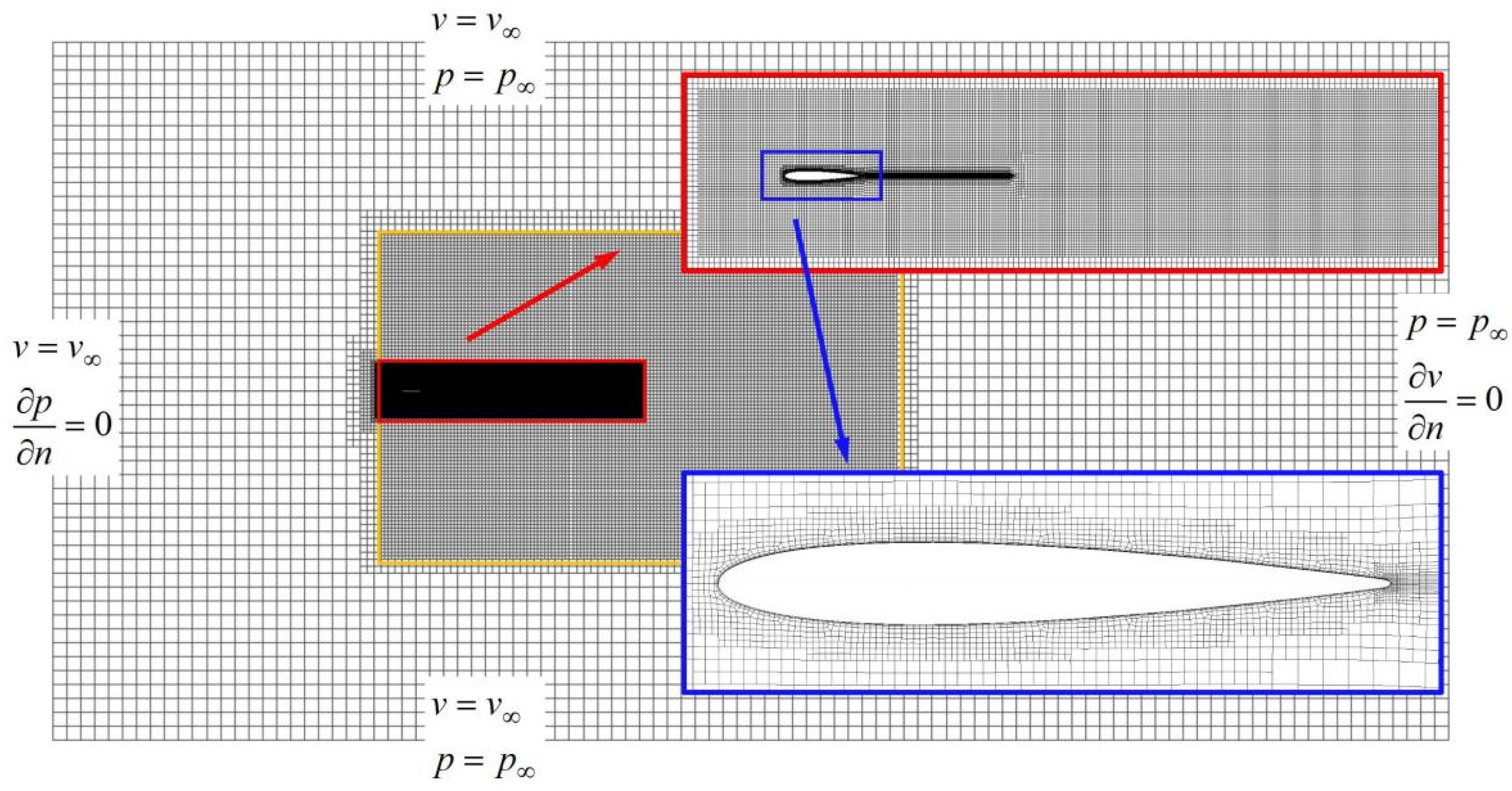
In this paper, the CFD software, FINE/Marine (a software package of NUMECA company, Brussels, Belgium; EURANUS solver is developed by European Space Agency, Paris, France), is used to investigate the hydrodynamic performance of flapping foil propulsor. The simulation uses dynamic mesh to simulate the moving object. The setting methods of boundary conditions are shown in Figure 6. The boundary condition of foil surface is set as the non-slip wall boundary to simulate the boundary layer flow. Four outside boundaries of the computational domain are set as far-field boundaries, in which the upper, lower, and right boundaries are given velocity and pressure, and the left boundary is given velocity and extrapolated pressure.
The octree mesh is adopted with local mesh refinement. As shown in Figure 6, the simulation is carried out in a computational domain of 25c × 50c, with a uniform domain of 10c × 20c (yellow rectangle in Figure 6), around the foil in which the maximum mesh size is less than 1/23c. Moreover, in order to accurately simulate the pressure and velocity gradient on the foil surface, as well as the separated vortex in the trail, further mesh refinement is carried out on the foil surface and wake region. The size of the refinement region which is shown as red rectangles is about 2c × 10c, in which the maximum mesh size is less than 1/25 of the chord length. The optimization of the near-wall mesh of the foil is shown in the blue rectangles in Figure 6, in which the maximum mesh size is less than 1/27 of the chord length. The total grid number is about 85,000. The near wall mesh is refined to ensure that the y+ value is about 1.0 and no wall function is used.
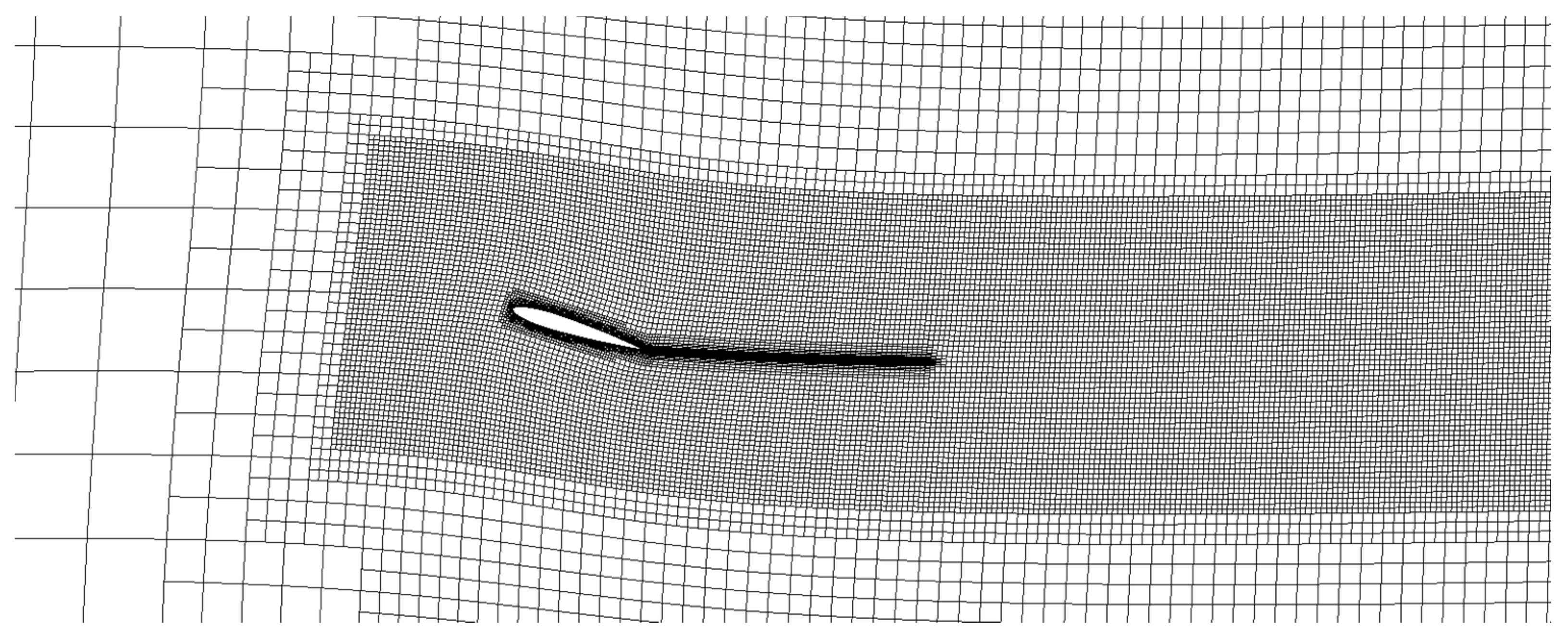
In order to adapt to the large-scale motion of the foil, rigid translation combined with elastic twist grids is adopted in the calculation, as shown in Figure 7. The simulation results of different grid sizes show that when the densified region is unchanged the fine-tuning of the grid size has little effect on the performance of the foil. The final mesh size selected in this paper is proven to be applicable, which can clearly resolve the vortex in the flow field.
The two-dimensional viscous flow is simulated which used Menter’s k-ω shear-stress transport turbulent model [27], and the governing equations can be written as follows:
where Ω is the element volume; is the flow velocity; is velocity component; is the displacement velocity of element surface; is the sum of viscous stress and Reynolds stress and P is the pressure; is the density of water; Sj is the components of area vector; and is the area vector of element surface.
4. Validation and Verification
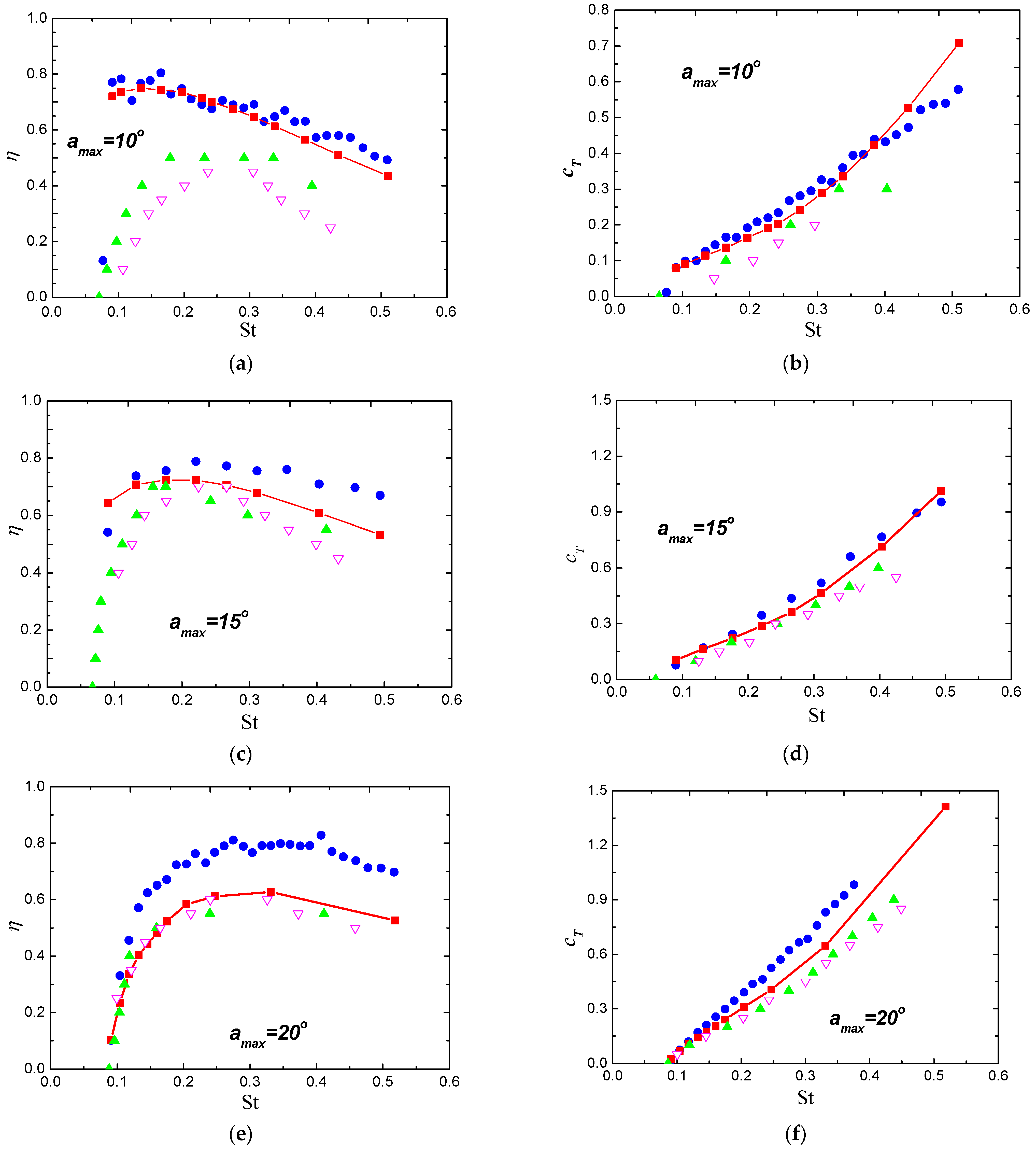
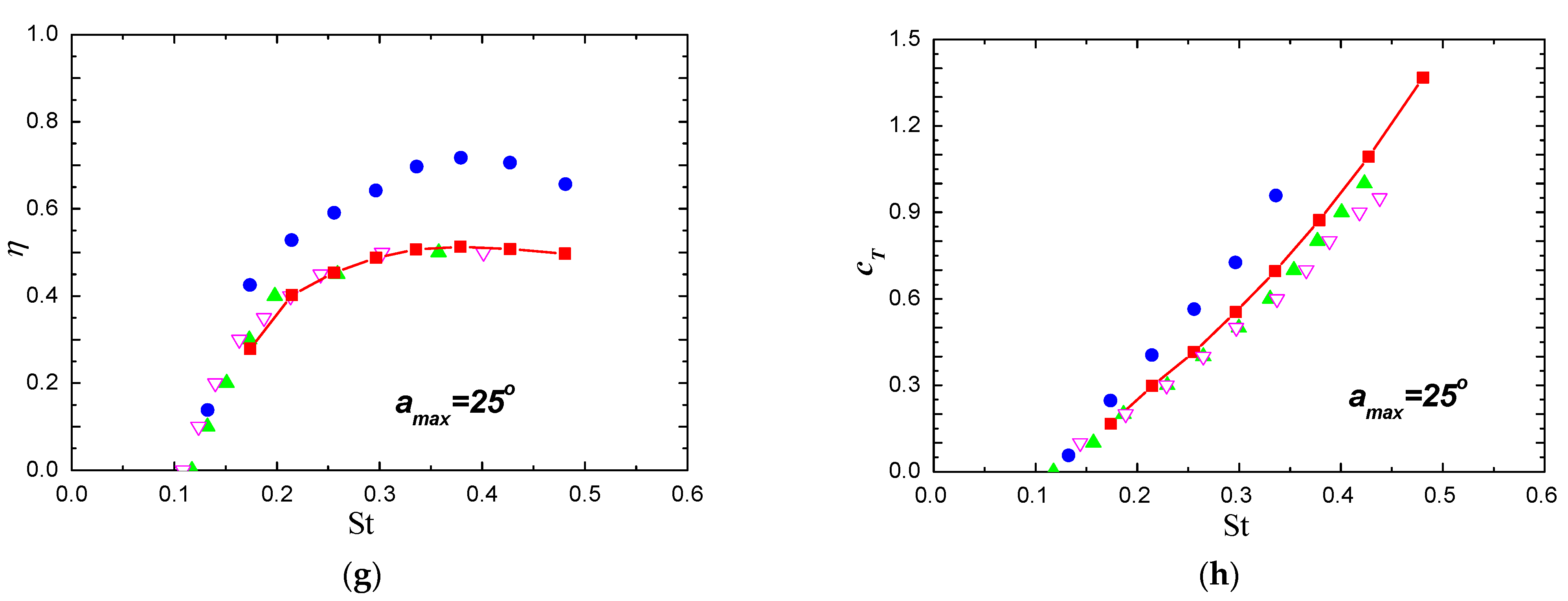
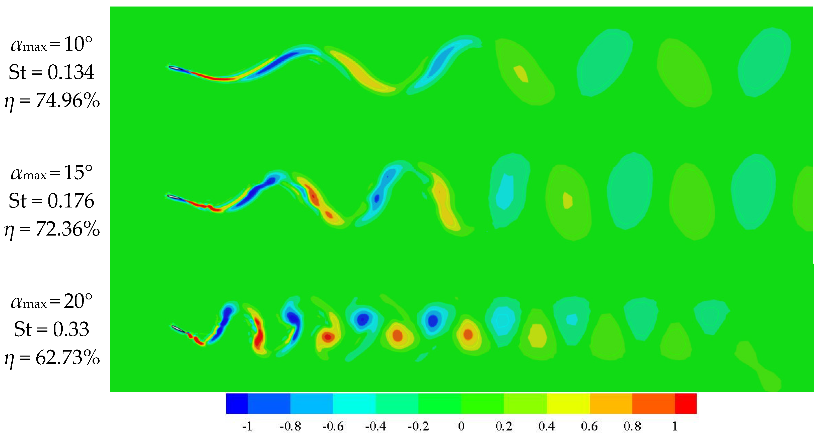
In order to validate the numerical method used in the current work, selected benchmark conditions in Anderson’s [3], Read’s [11], and Schoveiler’s [4] experiments are simulated, in which a rigid two-dimensional NACA 0012 airfoil is used. The heave amplitude-to-chord ratio y0/c is 0.75, and the pitching axis is 1/3 chord from the leading edge of the airfoil. The comparisons are shown in Figure 8. These three papers are from the same laboratory with the same foil working in similar conditions, but the results of the three papers are not consistent, which shows that the research in this area has room to develop. It can be seen from Figure 8 that when the maximum AOA αmax is 10°, the present numerical results agree well with the previous Anderson’s experiment results; when αmax is 25°, the results in this paper are in good agreement with Read and Schoveiler’s work; when αmax is 15° and 20°, the results in this paper are roughly in the middle of the previous three experimental results. Moreover, vorticity fields of some higher efficiency points are shown in Figure 9. The vortex street in the wake flow can be clearly observed from the calculation results.
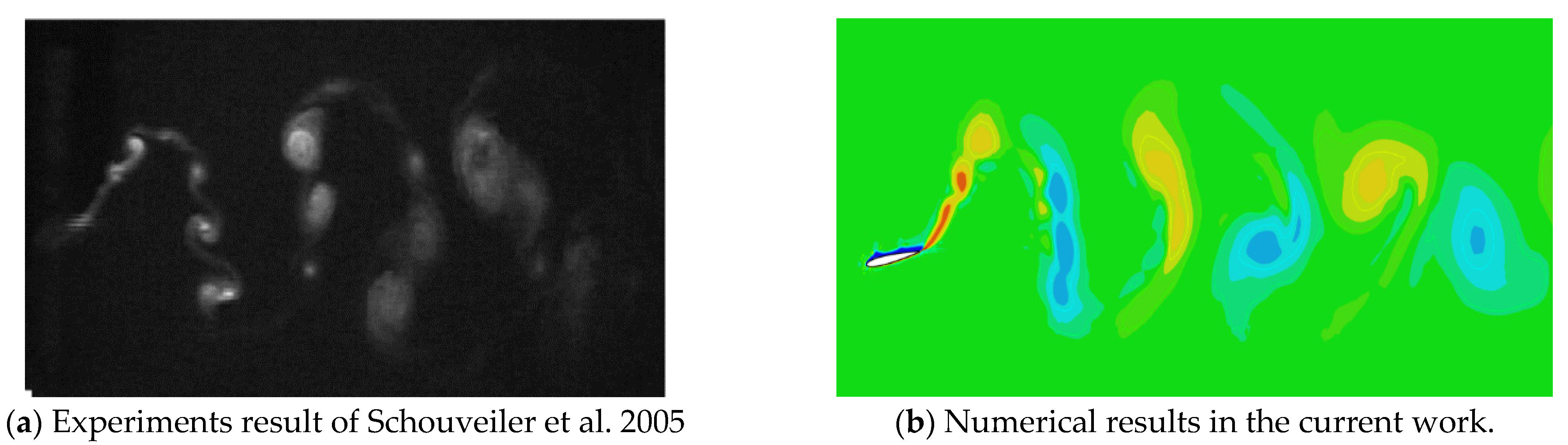
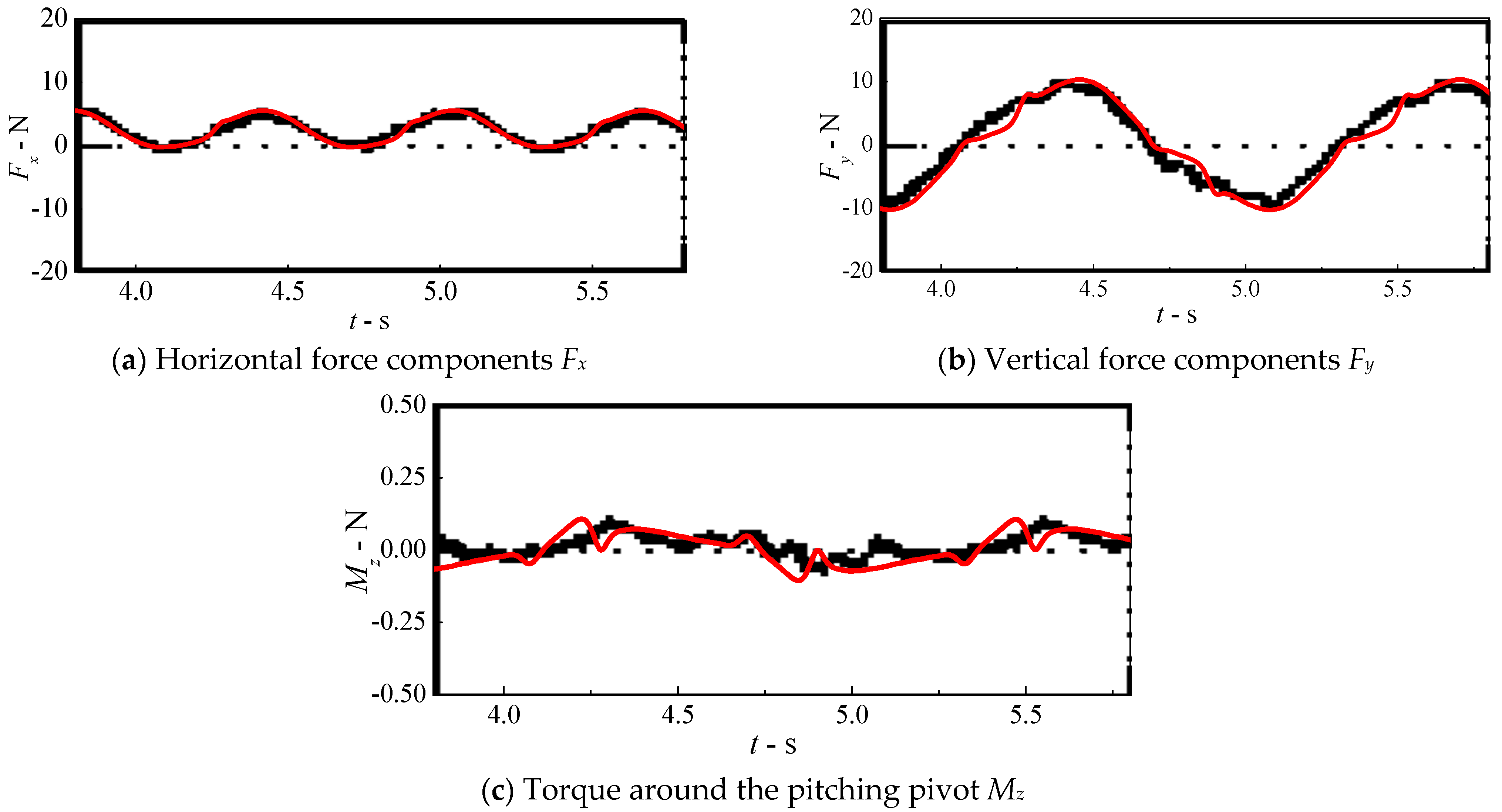
In order to validate the numerical method used in the current work, the calculation results under the same condition have also been compared with data from those experiments results, as described by Schoveiler [4]. Figure 10 is vorticity pattern visualized in the foil wake for St = 0.45, f = 1.2 Hz, amax = 20°. The experimental and the calculated results are compared and shown in Figure 10a,b separately, which agree with each other. In addition to qualitative comparison, we also compared the force measurements in Figure 11, Fx, Fy and Mz for St = 0.3, f = 0.8 Hz, amax = 20°, which demonstrates the accuracy of the simulation.
5. Results and Analysis
5.1. Effects of Harmonic Heaving and Pitching Amplitude
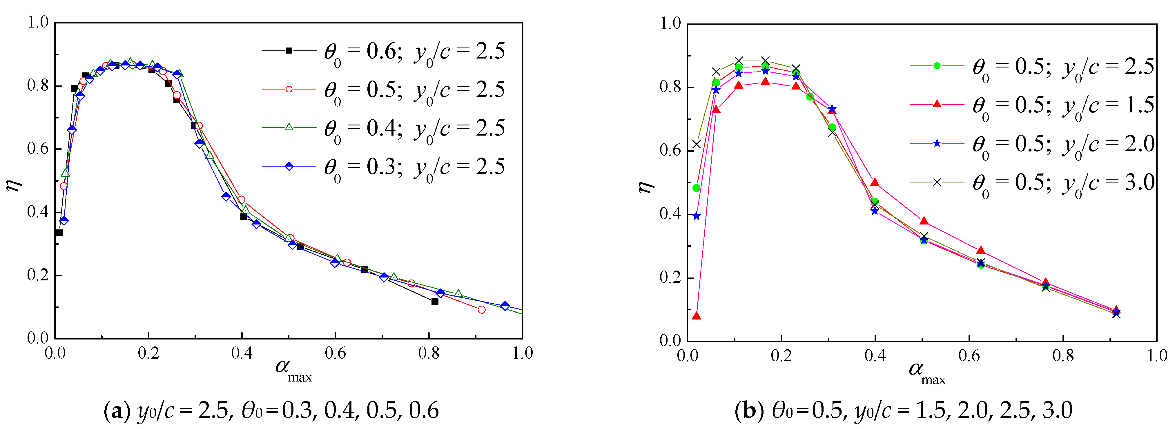
As mentioned before, the AoA is one of the main parameters that affect the flapping foil efficiency [3,19,28]. With different heaving amplitudes and different pitch amplitudes, the efficiency varies with the resulted AoAs for flapping foils with harmonic motion. Figure 12 presents a parametric study for the effect of maximum AoAs on the efficiency with varying heave and pitch motions. The heave and pitch motions in this session are all simple harmonic with a 90° phase difference and the distance from the pitching center from the leading-edge of the foil, S, is 0.
Through the analysis of many working conditions, a more universal relationship between the maximum AoA and efficiency is obtained in this paper. Firstly, from Figure 12a, it appears that when the heave amplitude-to-chord ratio y0/c is fixed at 2.5, the efficiency curves under different pitching amplitude θ0 almost coincide with each other. That is, pitching amplitude θ0 has little impact on the highest efficiency point. Then, when pitching amplitude θ0 is not changed, Figure 12b shows that the maximum efficiencies increase obviously with the increase of the heave amplitude-to-chord ratio y0/c, although the four efficiency curves are basically the same. The maximum efficiency value gains an increase from 81.7% to 88.4%. Finally, through the analysis of many working conditions, a more universal relationship between the maximum angle of attack and efficiency is obtained. In Figure 12, the curves trend of efficiency with the AoA are basically the same under various conditions. When the maximum AoA αmax is between 6° and 12°, the efficiency value reaches the maximum. The results show that αmax plays a more important role in foil efficiency than pitch and heave amplitude, which is in good agreement with previous research results [3,10,18,19,28], and the regularity is clearer in this paper.
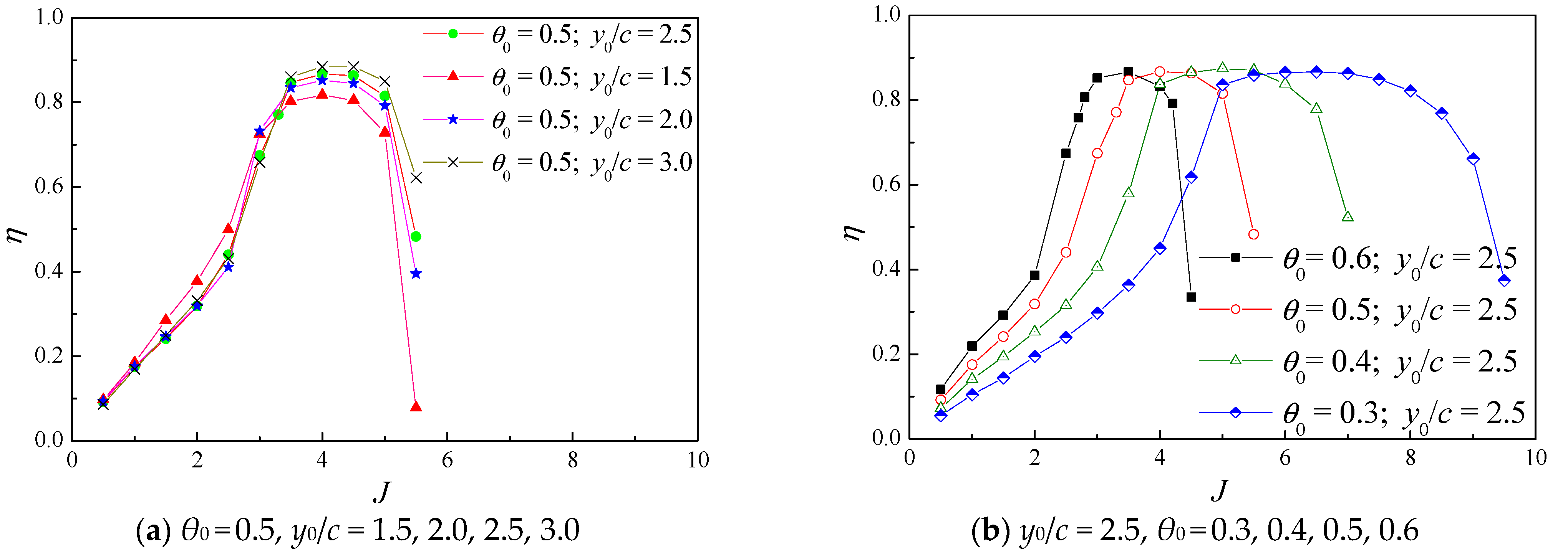
For the convenience of engineering application and comparison with the propeller, this part refers to the expression of Floc’h [5] on the advance coefficient J of the flapping foil propeller. The propulsion efficiency η and advance coefficient J under different heaving amplitudes and pitching angles are calculated according to Formula (5), as shown in Figure 13. It can be seen from Figure 13a that when the pitching amplitude θ0 is constant as 0.5, the efficiency curves under different heave amplitude-to-chord ratio y0/c almost coincide with each other. That is, the influence of the heaving amplitude on the advance coefficient J is small. However, in Figure 13b, when the heave amplitude-to-chord ratio y0/c is fixed, the change of pitching amplitude θ0 has a much larger influence on the advance coefficient J. On one hand, when the pitching amplitude becomes smaller, the maximum efficiency point of the flapping foil propeller deviates to a higher advance coefficient J. On the other hand, compared with the case of the larger pitching amplitude θ0, the range of maximum efficiency with a smaller pitching amplitude θ0 is much larger. Since the ship and vehicle usually work at a speed close to the propeller’s highest efficiency, a smaller pitching amplitude θ0 means a larger working range.
To sum up, the existing research results of simple harmonic motion parameters in this part show that the maximum AoA αmax has the greatest impact on flapping foil efficiency, and the efficiency curves at different maximum AoA have obvious regularity.; Changing the heaving amplitude y0 can also contribute to the improvement of efficiency, while the pitching amplitude θ0 has little impact on the highest efficiency point, but it has practical significance for the speed and working range of the ship and vehicle in the actual working condition.
5.2. Effect of Phase Difference
Apart from the AoA and amplitude of heaving and pitching, the phase difference between the heaving and pitching motions and the pivot location are two other important parameters affecting the performance of flapping foils [3,11,29,30,31,32,33,34]. However, most of the previous work only focused on these two parameters separately and ignored the relationship between them. Here, the phase difference is considered not only related to the heaving amplitude, but also to the pivot location of the foil. According to the motion of the flapping foil, the equivalent relations between phase difference and pivot location will be given in this section. In addition, a further set of numerical simulations were made to investigate the propulsive efficiency when the phase angle between the heave and pitch oscillations is varied.
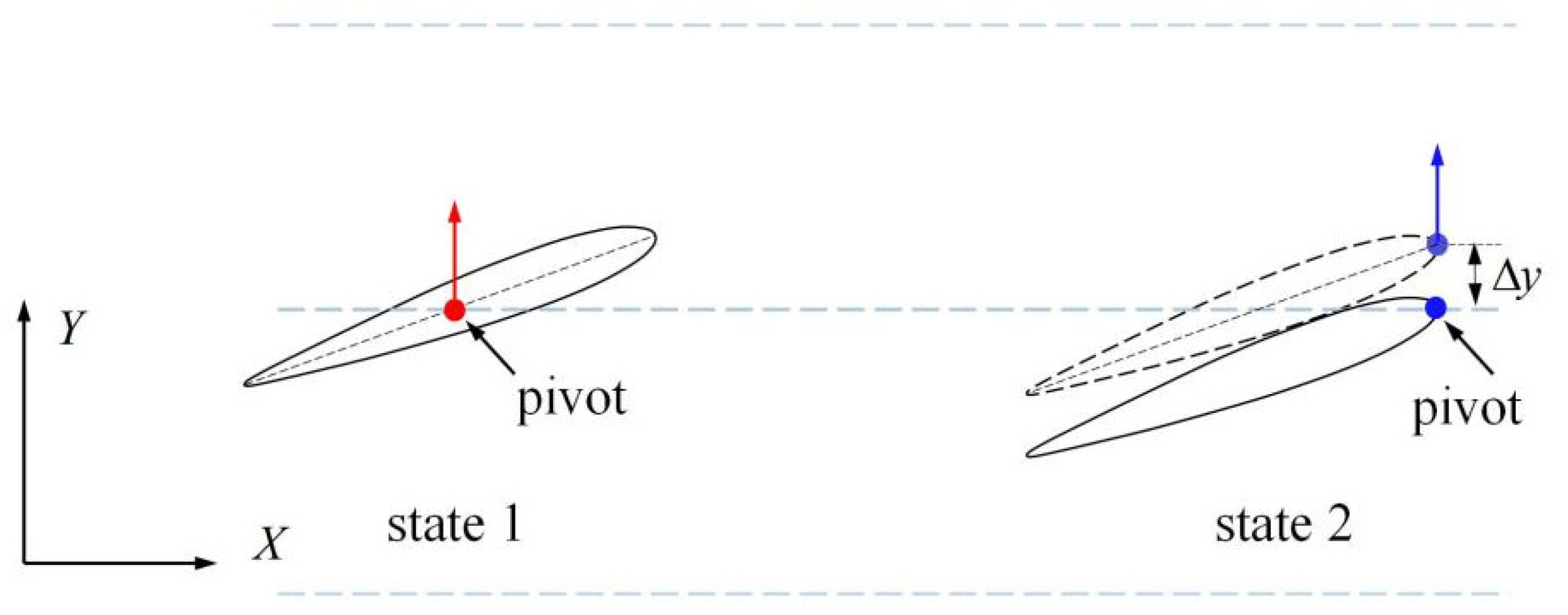
The phase difference is related to the pivot location of the flapping foil, and the relationship between them can be obtained from the geometric relationship. As shown in Figure 14, there are two sample states. The first one is a flapping foil with a phase difference φ = 90°, which is called “state 1”, and its pivot is located at the 1/2 chord length (as shown in the red dot). At this time, t = nT (whole period), the heaving amplitude y = 0, and the pitching angle θ is the maximum value (θ = θ 0). Under the assumption that the motion curves of each point on the foil are approximately harmonic, state 1 of the flapping foil can be also equated to another case. its pivot is at the leading edge (as shown in the blue dot in Figure 14), but at this time, the heaving motion is at the time of t = nT + Δt, while the pitching motion is at the time of t = (n + 1/4)T. That is, at this time, the phase difference φ = 90° − 2πfΔt, which is called “state 2” here. The foils in these two states have different phase differences and pivot locations, but they are in the same state. According to the above analysis, reducing the phase difference could be equivalent to moving the pivot position towards the leading edge.
Δs is defined as the displacement of the pivot in the chordwise direction, and it is positive in the tailing edge direction. Δφ is defined as the change of the phase difference between the two states of the foil. Compared with state 1, state 2 is completely equivalent, but the change of phase difference Δφ = −2πf Δt, and the pivot displacement Δs = −c/2. The relationship between Δs and Δφ is derived from the geometric relationship as follows. As shown in Figure 14, the distance between the leading edge and the center line Δy can be written as follows:
According to the heaving motion (Equation (1)), it can be obtained that Δt is
When Δy/y0 is small, there is an approximate relationship
That is, according to the motion law of the flapping foil, approximate relations of the four parameters including the phase difference, heave amplitude, pitching angle and rotation axis position are given as follows:
In order to verify the correctness of Equation (20), and based on this formula, we could further stimulate the propulsion efficiency, and eight groups of comparison conditions are set according to Equation (20), as shown in Table 1.
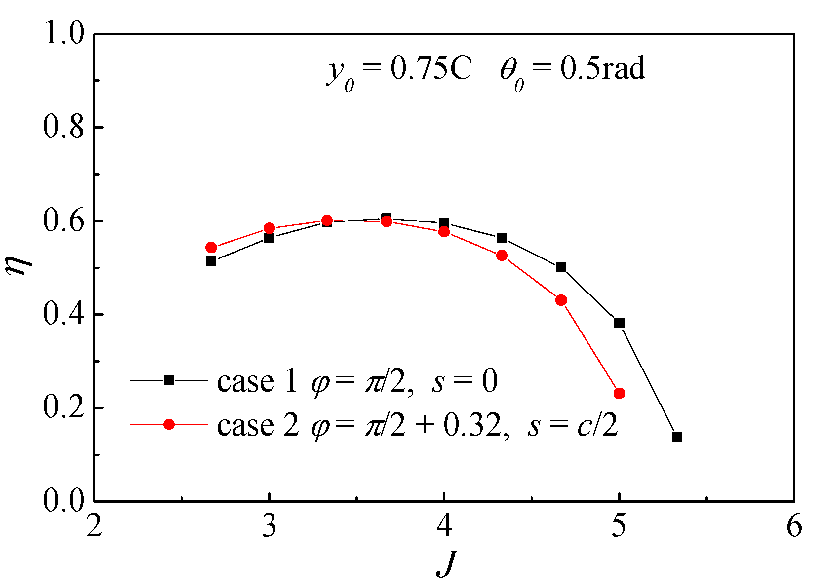
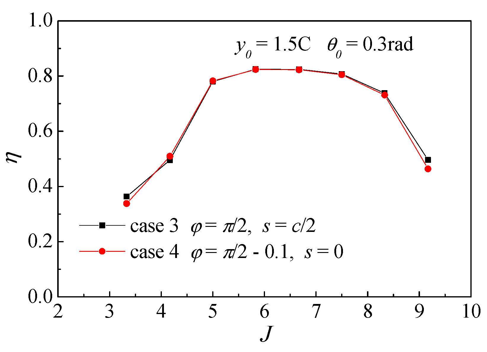
Firstly, the reliability of this formula is verified by comparing the first four working conditions. Case 1 and case 2 are compared to verify the accuracy of the equivalent formula under the condition of larger pitching angle and smaller heaving amplitude, which is shown in Figure 15. Case 3 and case 4 in Figure 16 are chosen to verify the accuracy of the equivalent formula under the condition of smaller pitching angle and larger heaving amplitude. The propulsive efficiency curves of the first two cases are shown in Figure 15. It is found that the efficiency curves of the two cases are slightly different, but the maximum efficiency value of them is the same. While, in the next two cases, the rotating axial moves toward the leading- edge direction, and the phase angle is reduced proportionally. It can be seen from Figure 16 that the efficiency curves of the two are almost overlapped with each other, that is, the working conditions of Case 3 and Case 4 are practically identical.
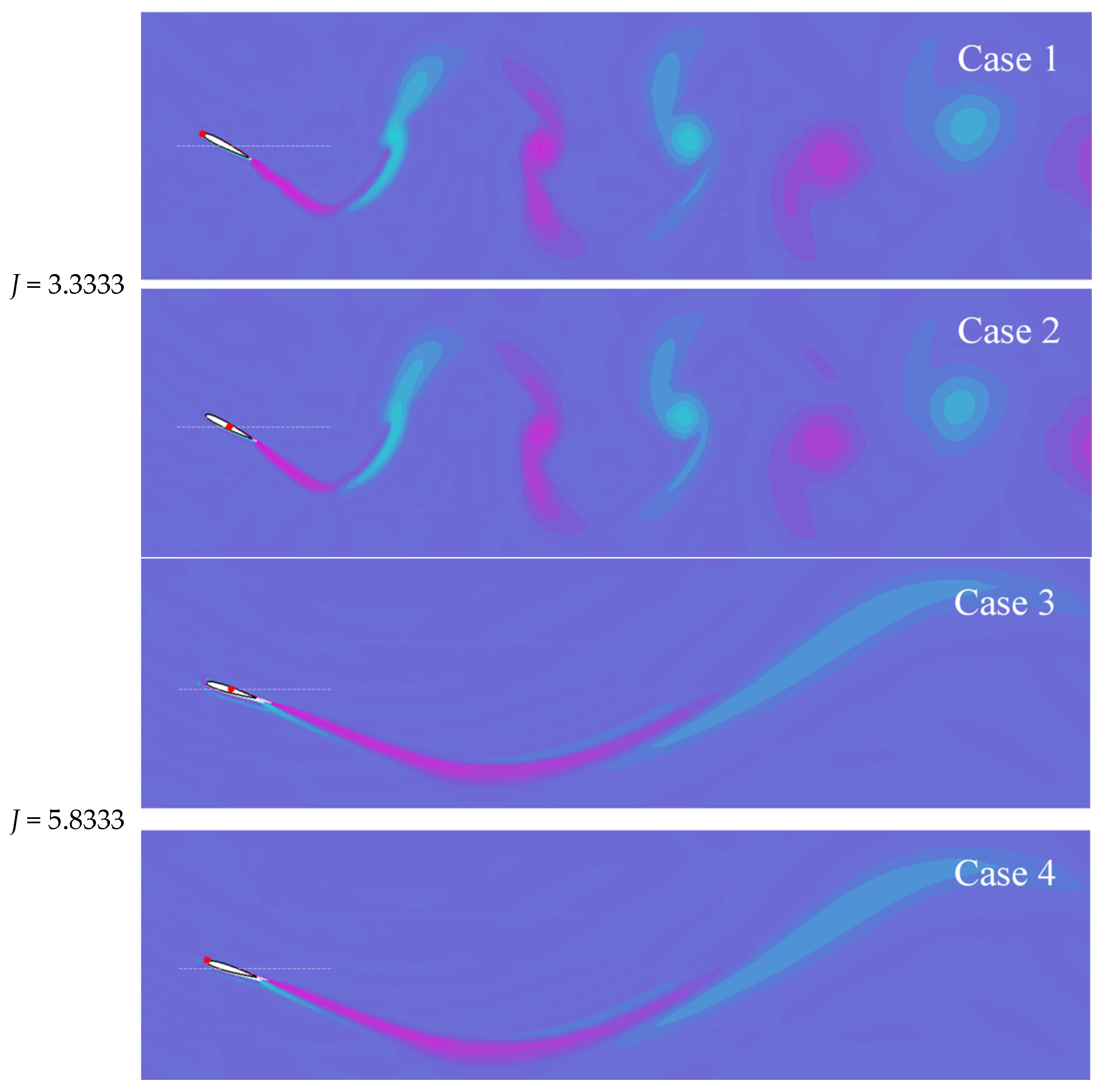
Figure 17 shows the wake flow field under these four verification conditions when the midpoint of the foil is at the equilibrium position. The red dot in the figure shows the pivot center position of the foil. As can be seen from Figure 17, the wake flow fields of Case 1 and Case 2 with different pivot positions and phase difference obtained by formula 20 are almost the same. A comparison of the results of Case 3 and Case 4 also shows the consistency between the two foils. However, the foils of Case 3 and Case 4 are leaving a narrower wake comparing to the previous two cases, which is consistent with the conclusion that the propulsion efficiency of these two Cases is higher than that of the first two cases. From the comparison results above, it can be seen that Equation (20) which is constructed in this chapter is applicable for the four parameters, and it is more applicable and accurate when the pitching angle is smaller, and the heaving amplitude is larger.
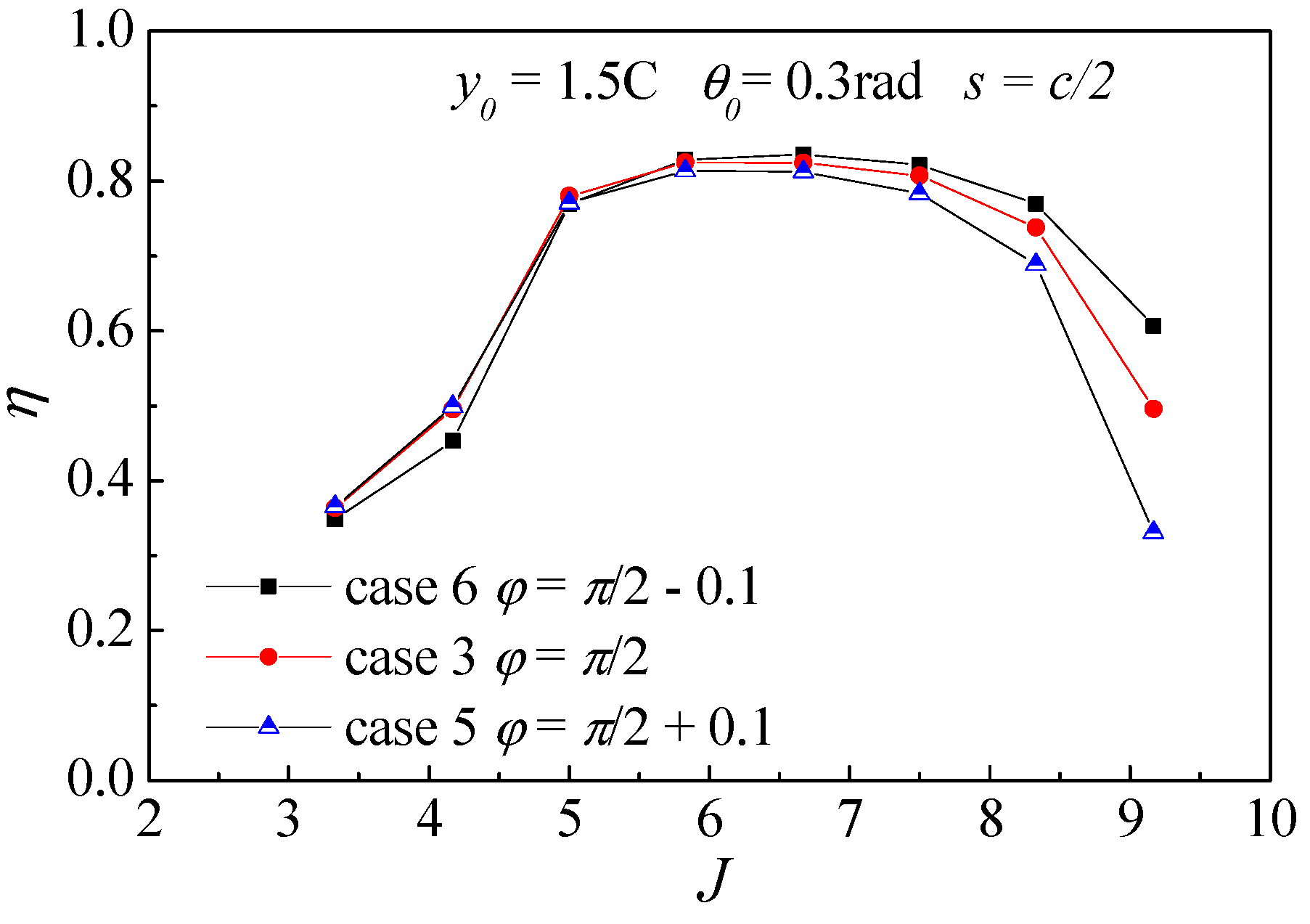
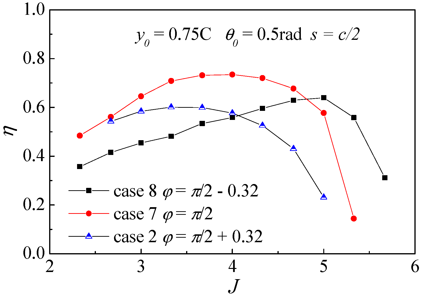
Then, the influence of phase difference on efficiency is further analyzed through the comparative study of the latter six cases. As shown in Figure 18, the comparison of Case 3, Case 5 and Case 6 shows the effect of phase difference on efficiency under smaller pitching angle and larger heaving amplitude; And Case 2, Case 7 and Case 8 are chosen for the comparative study of that under the condition of larger pitching angle and smaller heaving amplitude in Figure 19. From Figure 18, under the smaller pitching angle and larger heaving amplitude condition, the maximum efficiency of the three are almost the same, but the efficiency curve slightly deviates upward with the decrease of phase difference. That is, after exceeding the maximum efficiency point, under the same advance coefficient J, a smaller phase difference is conducive to maintaining higher efficiency. From the comparison results shown in Figure 19, It is found that the efficiency curve does not shift regularly with the increase of phase difference under large pitching angle and small heave amplitude condition. However, viewing the situation from a whole, the maximum efficiency point is gradually shifted to the left with the increase of phase difference, and when the phase difference is 90°, the peak efficiency is the highest. From the comparison of the above two groups, we can see that the effect of phase difference on efficiency is also related to the heaving amplitude and pitching angle, and there is no exact rule. Further analysis should be made according to the specific situation in the future.
5.3. Effect of Anharmonic Motion
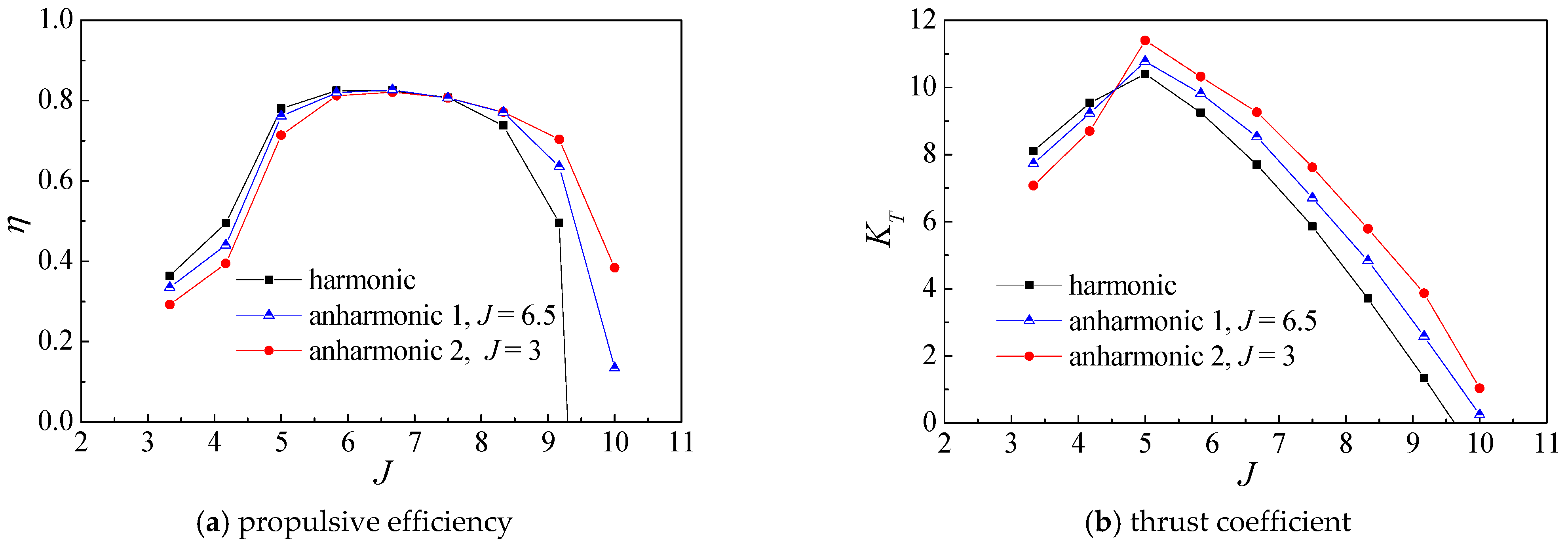
According to the previous analysis in Section 2, two anharmonic pitch motion trajectories under the given heave motion curve and a plumper AoA curve are constructed in Figure 3. The two anharmonic pitching angle trajectories are designed at the working points of J = 6.5 and J = 3, respectively. The parameters are set as follows: y0/c = 1.5, s = c/2, φ= π/2, θ0 = 0.3rad. The foil propulsive efficiency and thrust coefficient of these three different pitching angle trajectories are compared, and the results are shown in Figure 19.
Firstly, it is found that from Figure 20a, no matter what the designed trajectory is, the maximum efficiency values are almost the same. This means that even if some scholars have concluded that the anharmonic motion trajectory could improve the propulsion efficiency and thrust coefficient of the foil under a certain working condition [19], the results of this paper show that this designed anharmonic motion is not helpful to further improve the foil propulsion efficiency under a series of working conditions close to the maximum propulsion efficiency 80%. Although the construction methods of anharmonic motion trajectories are different, similar conclusions have also been obtained in Hover’s research [18]. He pointed out that in terms of maximum efficiency the cases of square and sawtooth AoA profiles are largely indistinguishable from the case of harmonic heave motion. However, Figure 20b shows that the thrust coefficient of the anharmonic trajectory is higher than that of the simple harmonic trajectory under the condition of a large advance coefficient. It shows that the anharmonic trajectory design may be applied to the engineering which needs a large thrust.
It is worth mentioning that with an anharmonic trajectory the efficiency curve of the foil has a slow downward trend under the condition of a larger advance coefficient. And under the high advance coefficient J, the anharmonic motion trajectory (equivalent to plumper AoA curve) corresponds to higher efficiency; while at low advance coefficient J, the efficiency corresponding to the anharmonic motion trajectory is lower. The same conclusion can be drawn from the research results of Lu [24]. In other words, compared with the foil with a simple harmonic trajectory, the foil with the anharmonic trajectory can maintain high efficiency with a relatively wider working range, and help to improve the efficiency and thrust coefficients under the condition of high advance coefficient J.
From the above analysis of the influence of several parameters on efficiency, it is found that the effect of heaving amplitude on the highest efficiency is the most obvious. Increasing heave amplitude can significantly improve the foil propulsive efficiency. Considering that it is difficult to achieve too large heaving amplitude in engineering, this paper only analyzes the case of heaving amplitude of 3.0. Secondly, phase difference also has a significant influence on efficiency, but this effect is related to the reference working condition, which needs further study. Then, the pitching angle amplitude has little effect on the maximum efficiency value of flapping foil, while it will affect its optimal speed range. At last, the influence of the anharmonic pitching angle trajectory on the maximum efficiency is very small. Considering that there are many parameters in the construction of anharmonic motion trajectory, and the construction methods of various researchers are also different, which may lead to the difficulty of unified parameter design in engineering application. At the same time, it is relatively difficult to realize the anharmonic motion of flapping wing by using crank connecting rod mechanism. Therefore, this paper holds that it is not of great practical significance to study the use of anharmonic motion to further improve the propulsion efficiency, especially under the working conditions near the highest efficiency point.
5.4. Wake Field and Force Analysis
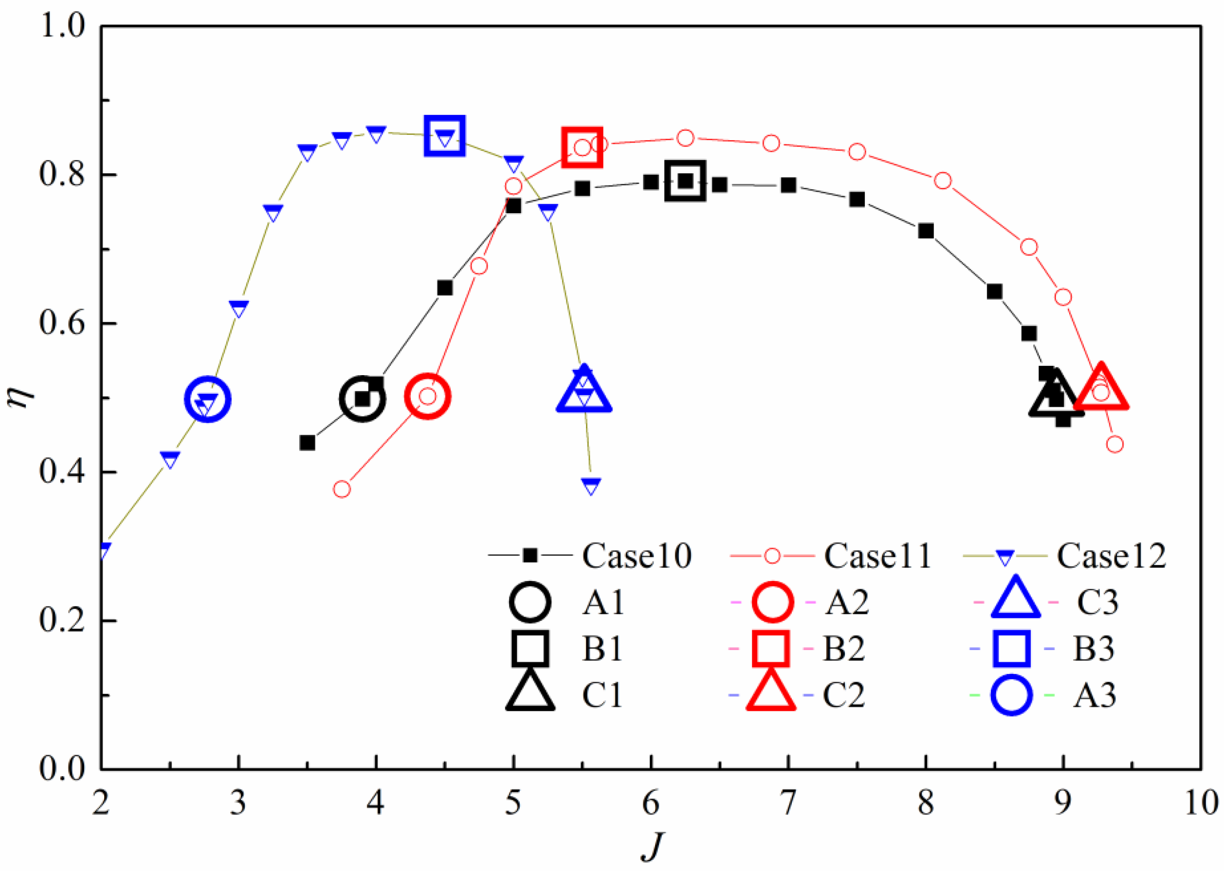
In order to further analyze the high-efficiency reason of flapping foil, this part discusses the wake field and the force on the foil. Three groups of high-efficiency cases are selected in this section for further study according to the previous research results. At the same time, the highest efficiency point, 50% efficiency point on the left side of the highest efficiency point and 50% efficiency point on the right side of the highest efficiency point are selected for flow field and force analysis, respectively. The selected three groups of parameters are shown in Table 2. Three efficiency curves and nine analysis points are shown in Figure 21.
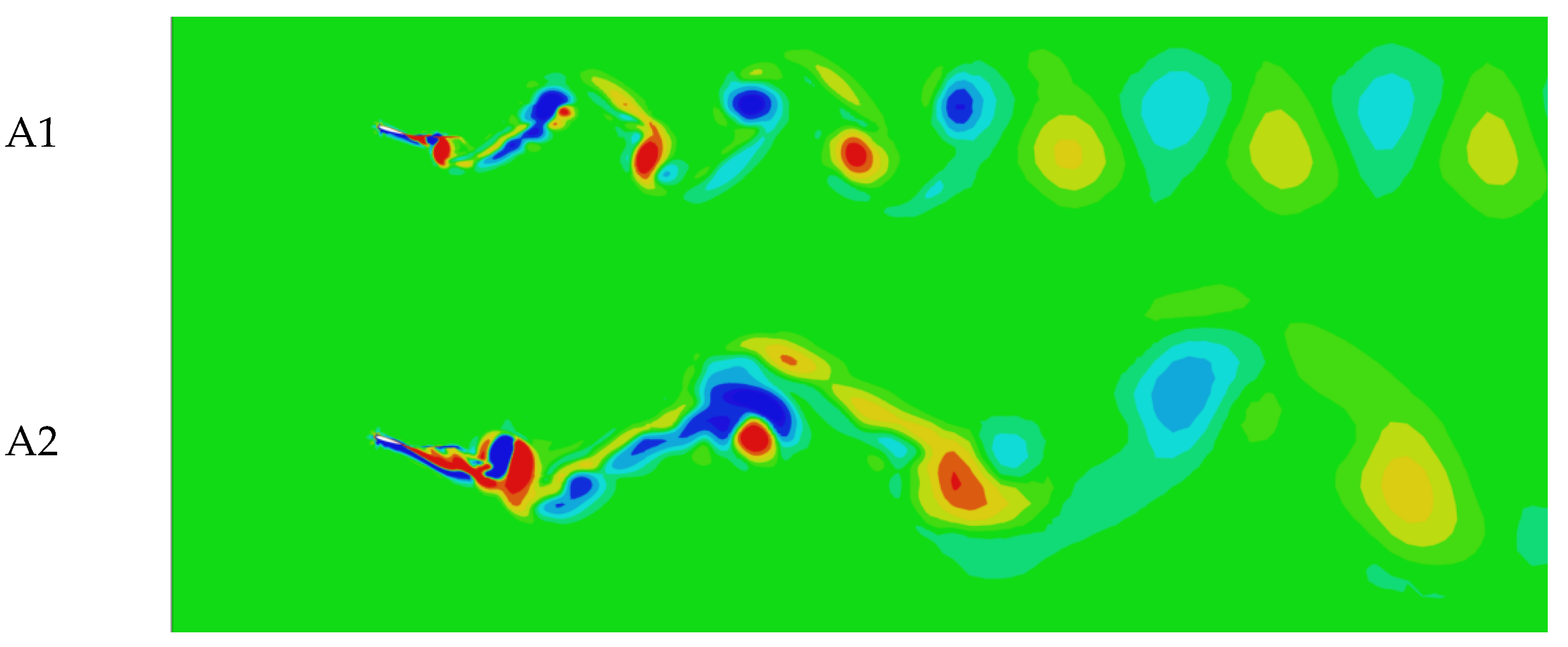
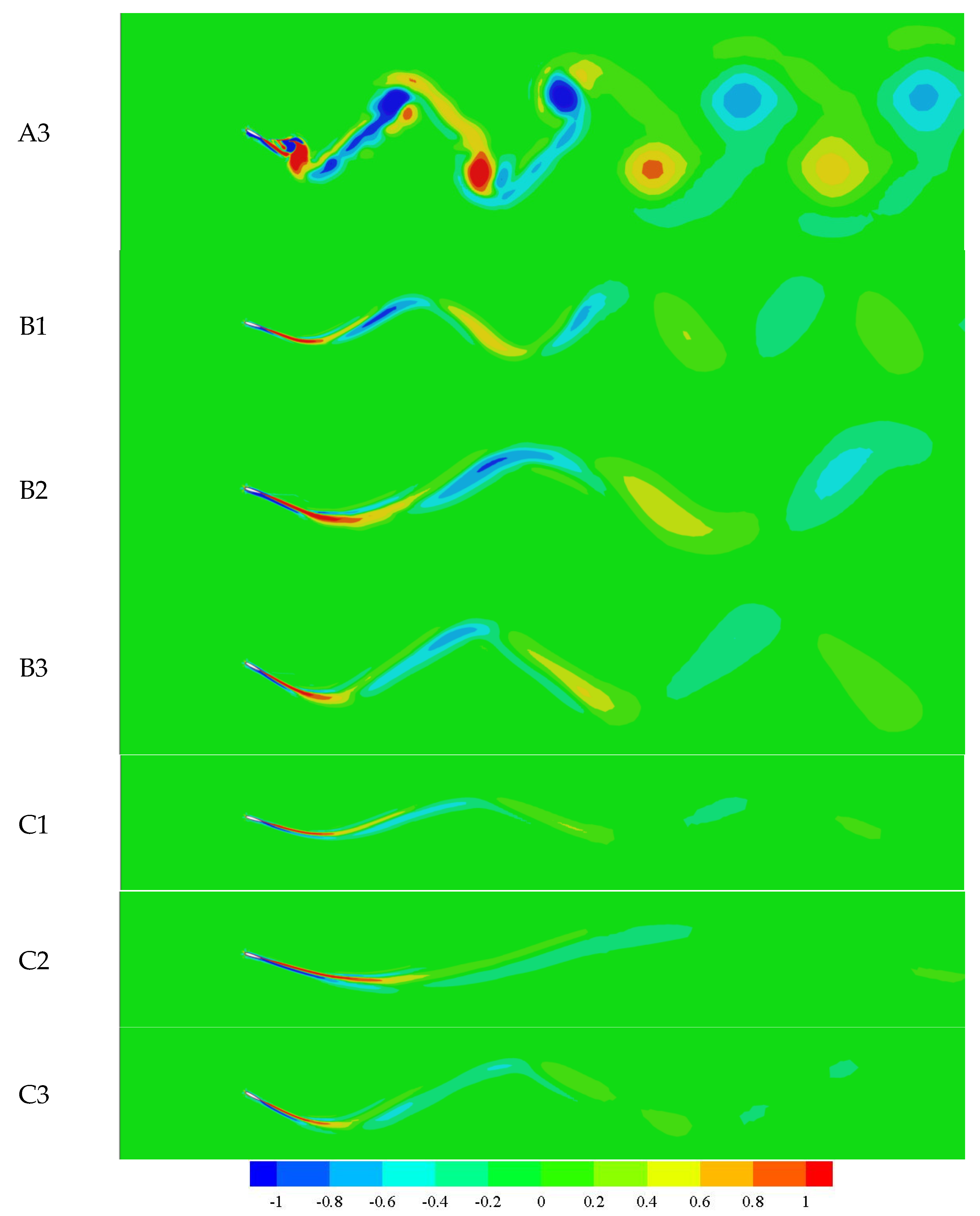
Firstly, the vorticity fields of nine analysis points from A1 to C3, which are shown in Figure 21, are compared in this section. From vorticity distribution contours of nine analysis points shown in Figure 22, it is easy to recognize that the wake vortex of A1, A2, and A3 points are stronger than that of the other six points, which may be the main reason for their low efficiency. In contrast, the wake loss of the other six points, B1 to B3 and C1 to C3, are smaller because of their narrow-banded tailing vortex structure. It should be noted that, although the tailing vortex structures of these six points are almost the same narrow-banded, the efficiencies of C1 to C3 are still not as high as that of B1 to B3, and their wake attenuation is much faster than points B1 to B3. The details remain to be discussed in the follow-up work.
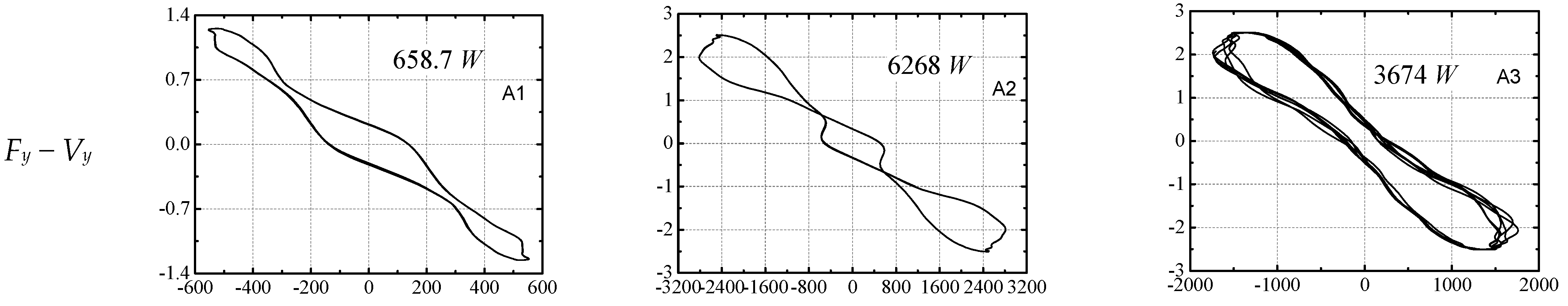
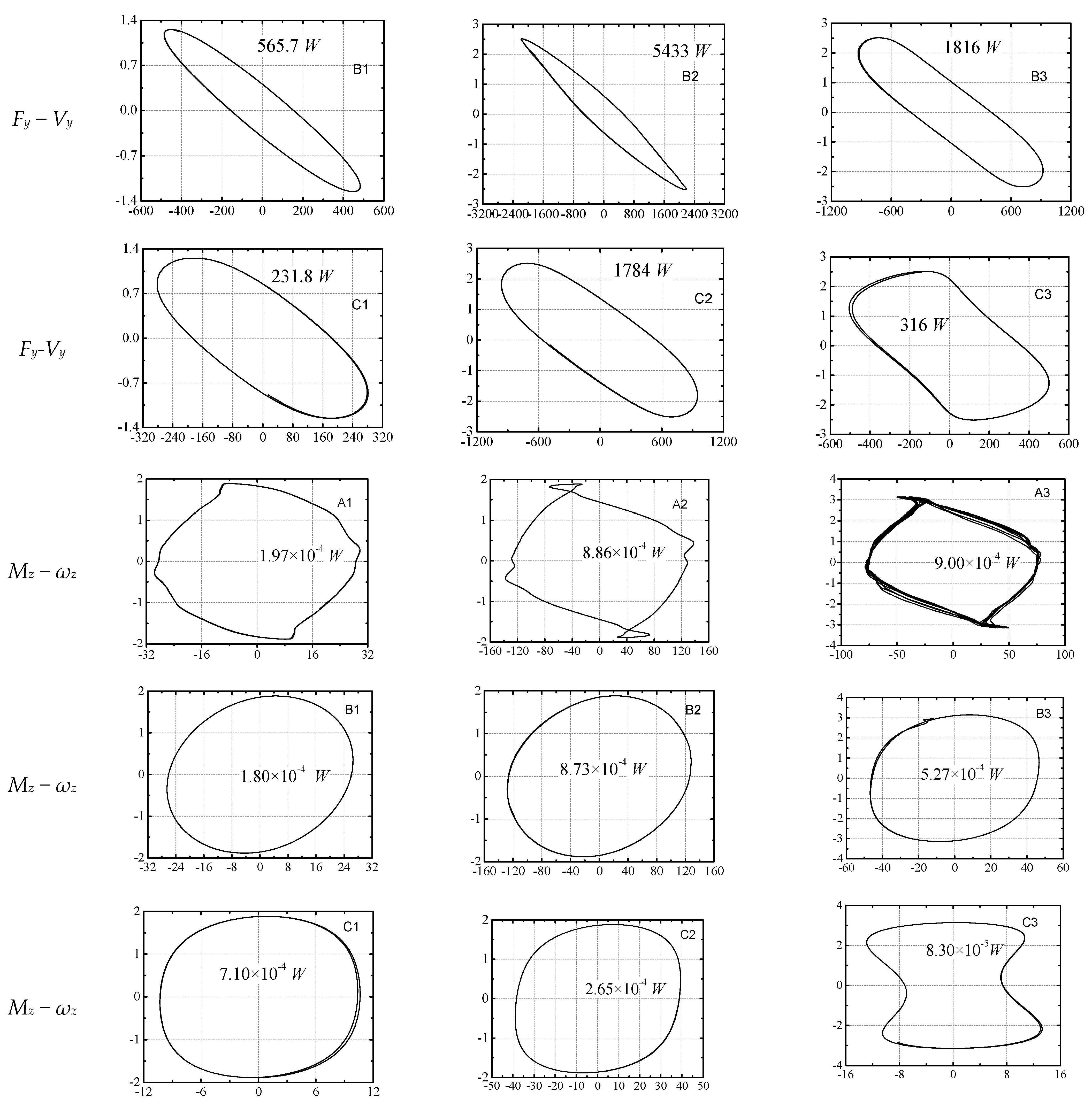
Next, the phase difference between the mechanical parameters and the velocity parameters are discussed. When the flapping wing moves at a constant speed, the calculation parameters that affect the efficiency value include not only the mechanical parameters Fx, Fy and Mz, but also the velocity parameters vy and ωz. These parameters fluctuate with time, so when calculating the product, the phase difference between the parameters has a great influence on the result. Figure 23 shows the Fy − vy and Mz − ωz phase diagrams of nine operating points, respectively. Viewing the situation from a whole, there is a certain phase difference between both Fy − vy and Mz − ωz. The phase difference between Fy and vy is small, while the phase difference between Mz and ωz is large, which is close to 90°. At the same time, the magnitude of Fyvy is much larger than that of Mzωz. The above two points show that the y-direction force generates more power in the input power, while the torque around the z-axis is almost no work. In order to compare the work performance more clearly, the average input powers in a period of nine operating points are also given in the Figure 23. It can be seen more clearly from the data that compared with the Y-direction force, the input power of the torque around the z-axis can be almost be ignored. Then, the Fy − vy and Mz − ωz phase diagrams of different working conditions are compared in detail. From the horizontal comparison of A1 to A3, not only their Fy − vy phase diagrams, but Mz − ωz phase diagrams are similar to each other. And the same phenomenon is also found in the phase diagrams of B1 to B3 and C1 to C3. It can be found that at the similar efficiency points the force characteristics of the flapping foil are similar. From the longitudinal comparison of A, B, and C, the phase diagram curve becomes smoother from A to C, that is, under the same motion parameter, with the increase of the speed coefficient, the time history curve of force is closer to the simple harmonic. At the same time, the phase difference between Fy and vy increases with the increase of the advance coefficient. However, efficiency is related to Fx and Fy, at the same time, we cannot draw specific conclusions from the analysis of Fy here.
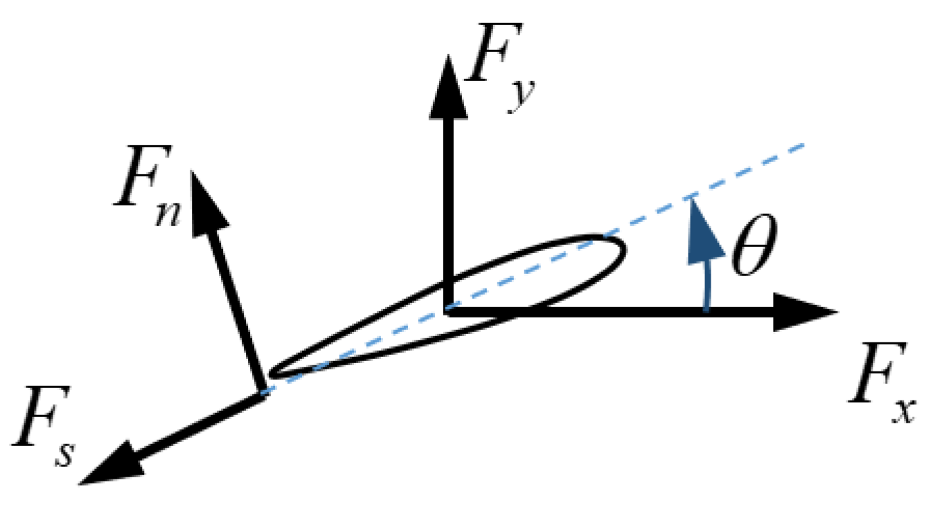
Then, according to the above analysis, when the parameters of the flapping foil are determined, the forces that affect the propulsion efficiency are only Fx and Fy. In previous studies, the forces on airfoil are usually divided into drag R along the relative inflow and lift L perpendicular to the relative inflow. However, since the inflow angle and attack angle of the flapping foil change at any time during the working process, its lift coefficient is also unstable, which is not only related to the AoA, but also related to the angular velocity of motion, so it is difficult to analyze according to the lift and resistance. In this paper, the forces on the airfoil are divided into Fs along the chordwise direction and Fn perpendicular to the chordwise direction for analysis. As shown in Figure 24, the relationship between the forces is shown as follows:
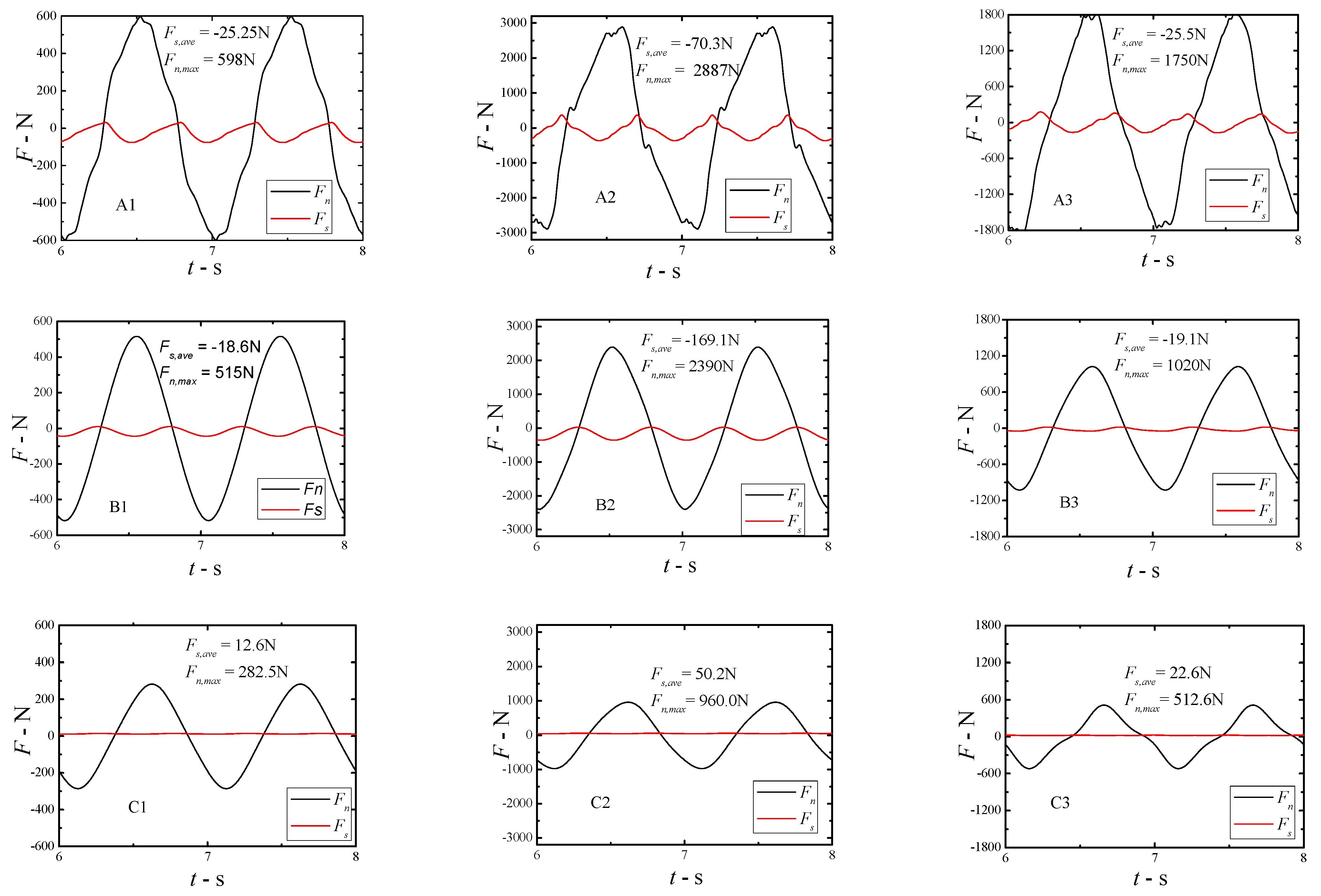
The Fs and Fn curves of nine working points calculated from the above formula are shown in Figure 25. First of all, it can be seen intuitively from the results that under any working condition, compared with the normal force Fn, the chord force Fs is very small and can be ignored. At the same time, we also found that under the same motion parameters, when the working point moves from A to C, the normal force Fn decreases gradually, while the efficiency does not decrease with the decrease of the normal force Fn, but reaches the peak at point B. At the same time, compared with A and C, the phase difference of the two forces at point B is much closer to 90. Therefore, comparing the different operating points of the same flapping foil, this paper cannot clear the relationship between Fn and the highest efficiency point yet. However, it can be determined that since Fs is smaller than Fn, the resultant force of Fx and Fy is mainly determined by Fn. Therefore, if the corresponding relationship between Fn and motion parameters can be determined, the efficiency under the motion parameters can be directly obtained. However, because there are many motion parameters that affect Fn, and the relationship between them is complex, this paper has not made an in-depth study; this part of the work will be gradually improved in future work. Finally, from the average value of Fs and the maximum value of Fn also given in Figure 25, it can be seen that at point C, the average value of chord force Fs is positive, which indicates the viscous resistance; while, at point A and point B, the average value of chord force Fs is negative, that is, the chord force points to the leading edge, which is a special phenomenon. According to the conventional imagination, the chord force of the airfoil should be along the flow direction, which is the result of the viscous effect, but in the flapping foil, we found that the force may be against the flow direction.
6. Conclusions and Future Direction
The propulsion performances of a rigid active flapping foil are investigated systematically in this work. The two-dimensional viscous flow over the flapping foil is simulated by the CFD method. The parameter analysis of the combined oscillating foil which includes both heaving and pitching motions with different motion parameters are discussed, including AoA, pitching angle, heaving amplitude, phase difference and trajectory.
- Based on the numerical results obtained, it is found that the maximum AoA αmax has the greatest impact on flapping foil efficiency, in the range of αmax from 6° to 12°, the flapping foil propeller can ensure high propulsion efficiency. The highest propulsion efficiency could be reached when the maximum AoA is around 9°.
- The effect of heave amplitude yo on the maximum efficiency value of flapping foil is obvious, and the maximum efficiency could reach as high as 87% when the heave amplitude-to-chord ratio y0/c is 3.0.
- The pitching amplitude θ0 has little impact on the highest efficiency point, but when introducing the anharmonic pitching motion it shows that it can maintain high efficiency with a relatively wider working range, and help to improve the efficiency and thrust coefficients under the condition of high advance coefficient J.
- An approximate relation of the four parameters including the phase difference, heave amplitude, pitching angle and rotation axis position is given. The phase difference effects the maximum efficiency of the flapping foil, but this effect is also related to the heaving amplitude, pitching angle and pivot location.
- The flow field and force characteristics of the flapping foil with different motion parameters are analyzed. It can be seen from the results that compared with the Y-direction force, the input power of the torque around the z-axis can almost be ignored. when the foil is swinging around the higher efficiency points, the foil is leaving a narrower wake compared to the other designs.
In summary, high-efficiency results are obtained for many combinations of the parameters and the investigation could help us to identify the range of the parameters providing high propulsive efficiency. The numerical results agree well with previous experimental measurements and, in addition, allow access to the velocity, vorticity fields as functions of space and time, and input power characteristics and the force characteristics, which in turn allows us to identify the underlying thrust production mechanisms more easily. Meanwhile, the discussion of pitching motion torsional energy dissipation in this paper could provide some basic theories for the design of semi-active foil propulsion, which is now a hot topic.
These findings are based on results obtained varying one parameter while keeping the other parameters fixed. Hence for definitive conclusions, a more exhaustive investigation of the parameters should be performed in the future. On the one hand, this paper gives the approximate relationship of four parameters: phase difference, heaving amplitude, pitch angle and rotation axis position, but because the influence of phase difference on efficiency is also related to heave amplitude and pitch angle, no exact law is obtained. Therefore, further analysis of various parameters can be made in this regard.; On the other hand, all the conclusions of this paper are based on the analysis results of numerical calculations, which can be verified by a series of experiments in the future work, enrich the test data of flapping foil, and further demonstrate the correctness of this paper. Furthermore, the mechanism of why the foil maximum efficiency is limited to about 85% has not been explored clearly. This task can be imagined to be very arduous. However, it is of great significance for foil- based flow structure, aerodynamic/hydrodynamic performance and energy collection efficiency.
Author Contributions
Conceptualization, J.Z. and L.M.; Methodology, D.Y. and J.Z.; Simulation, X.P. and M.L.; Validation, J.Z., W.S. and L.M.; Writing—original draft preparation, J.Z.; writing—review and editing, J.Z., W.S. and L.M. All authors have read and agreed to the published version of the manuscript.
Funding
The authors would like to thank the supports from National Natural Science Foundation of China (Grant No. 51309070, 51503051), Shandong Province Science and technology development plan item (Grant No. 2013GGA10065).
Institutional Review Board Statement
Not applicable.
Informed Consent Statement
Not applicable.
Data Availability Statement
Not applicable.
Conflicts of Interest
The authors declare no conflict of interest.
References
- Triantafyllou, M.S.; Triantafyllou, G.S. An efficient swimming machine. Scientific 1995, 272, 64–70. [Google Scholar] [CrossRef]
- Anderson, J.M. Vorticity Control for Efficient Propulsion; Massachusetts Institute of Technology: Cambridge, MA, USA, 1996. [Google Scholar] [CrossRef] [Green Version]
- Anderson, J.M.; Streitlien, K.; Barrett, D.S.; Triantafyllou, M.S. Oscillating foils of high propulsive efficiency. J. Fluid Mech. 1998, 360, 41–72. [Google Scholar] [CrossRef] [Green Version]
- Schouveiler, L.; Hover, F.S.; Triantafyllou, M.S. Performance of flapping foil propulsion. J. Fluid Mech. 2005, 20, 949–959. [Google Scholar] [CrossRef]
- Floc’h, F.; Phoemsapthawee, S.; Laurens, J.M.; Leroux, J.B. Porpoising foil as a propulsion system. Ocean Eng. 2012, 39, 53–61. [Google Scholar] [CrossRef]
- Zhang, X.; Su, Y.M.; Wang, Z.L. Numerical simulation of the hydrodynamic performance of an unsymmetrical flapping caudal fin. J. Hydrodyn. Ser. B 2012, 24, 354–362. [Google Scholar] [CrossRef]
- Ramamurti, R.; Geder, J.; Palmisano, J.; Ratna, B.; Sandberg, W.C. Computations of flapping flow propulsion for unmanned underwater vehicle design. AIAA J. 2012, 48, 188–201. [Google Scholar] [CrossRef]
- Politis, G.K.; Tsarsitalidis, V.T. Flapping wing propulsor design: An approach based on systematic 3D-BEM simulations. Ocean Eng. 2014, 84, 98–123. [Google Scholar] [CrossRef]
- Thaweewat, N.; Phoemsapthawee, S.; Juntasaro, V. Semi-active flapping foil for marine propulsion. Ocean Eng. 2018, 147, 556–564. [Google Scholar] [CrossRef]
- Wu, X.; Zhang, X.; Tian, X.L.; Li, X.; Lu, W. A review on fluid dynamics of flapping foils. Ocean Eng. 2020, 195, 106712. [Google Scholar] [CrossRef]
- Read, D.A.; Hover, F.S.; Riantafyllou, M.S. Forces on oscillating foils for propulsion and maneuvering. J. Fluids Struct. 2003, 17, 163–183. [Google Scholar] [CrossRef]
- Politis, G.K.; Tsarsitalidis, V.T. Simulating Biomimetic (Flapping Foil) Flows for Comprehension, Reverse Engineering and Design. Available online: https://www.researchgate.net/publication/268296496_Simulating_Biomimetic_flapping_foil_Flows_for_Comprehension_Reverse_Engineering_and_Design (accessed on 28 July 2021).
- Guglielmini, L.; Blondeaux, P. Propulsive efficiency of oscillating foils. Eur. J. Mech. B-Fluid 2004, 23, 255–278. [Google Scholar] [CrossRef]
- Floryan, D.; Buren, T.V.; Rowley, C.W.; Smits, A.J. Scaling the propulsive performance of heaving and pitching foils. J. Fluid Mech. 2017, 822, 386–397. [Google Scholar] [CrossRef] [Green Version]
- Schnipper, T.; Andersen, A.; Bohr, T. Vortex wakes of a flapping foil. J. Fluid Mech. 2009, 633, 411. [Google Scholar] [CrossRef] [Green Version]
- Andersen, A.; Bohr, T.; Schnipper, T.; Walther, J.H. Wake structure and thrust generation of a flapping foil in two-dimensional flow. J. Fluid Mech. 2017, 812, R4. [Google Scholar] [CrossRef] [Green Version]
- Lin, X.; Wu, J.; Zhang, T. Performance investigation of a self-propelled foil with combined oscillating motion in stationary fluid. Ocean Eng. 2019, 175, 33–49. [Google Scholar] [CrossRef]
- Hover, F.S.; Haugsdal, Ø.; Triantafyllou, M.S. Effect of angle of attack profiles in flapping foil propulsion. J. Fluids Struct. 2004, 19, 37–47. [Google Scholar] [CrossRef] [Green Version]
- Xiao, Q.; Liao, W. Numerical investigation of angle of attack profile on propulsion performance of an oscillating foil. Comput. Fluids. 2010, 39, 1366–1380. [Google Scholar] [CrossRef]
- Berman, G.J.; Wang, Z.J. Energy-minimizing kinematics in hovering insect flight. J. Fluid Mech. 2007, 582, 153–168. [Google Scholar] [CrossRef] [Green Version]
- Xiao, Q.; Liao, W.; Yang, S.C.; Peng, Y. How motion trajectory affects energy extraction performance of a biomimic energy generator with an oscillating foil. Renew. Energy 2012, 37, 61–75. [Google Scholar] [CrossRef] [Green Version]
- Xie, Y.H.; Lu, K.; Zhang, D. Investigation on energy extraction performance of an oscillating foil with modified flapping motion. Renew. Energy 2014, 63, 550–557. [Google Scholar] [CrossRef]
- Lu, K.; Xie, Y.H.; Zhang, D.; Lan, J.B. Numerical investigations into the asymmetric effects on the aerodynamic response of a pitching airfoil. J. Fluids Struct. 2013, 39, 76–86. [Google Scholar] [CrossRef]
- Lu, K.; Xie, Y.; Di, Z. Nonsinusoidal motion effects on energy extraction performance of a flapping foil. Renew. Energy 2014, 64, 283–293. [Google Scholar] [CrossRef]
- Amiralaei, M.R.; Alighanbari, H.; Hashemi, S.M. Flow field characteristics study of a flapping airfoil using computational fluid dynamics. J. Fluids Struct. 2011, 27, 1068–1085. [Google Scholar] [CrossRef]
- Chao, L.M.; Pan, G.; Zhang, D.; Yan, G.X. Numerical investigations on the force generation and wake structures of a nonsinusoidal pitching foil. J. Fluids Struct. 2019, 85, 27–39. [Google Scholar] [CrossRef]
- Menter, F.R.; Rumsey, C.L. Assessment of two-equation turbulence models for transonoc flows. AIAA Fluid Dyn. Conf. 1994, 94, 2343–2361. [Google Scholar] [CrossRef]
- Mandujano, F.; Málaga, C. On the forced flow around a flapping foil. Phys. Fluids. 2018, 30, 061901. [Google Scholar] [CrossRef]
- BØ kmann, E.; Steen, S. Experiments with actively pitch-controlled and springloaded oscillating foils. Appl. Ocean Res. 2014, 48, 227–235. [Google Scholar] [CrossRef]
- Moriche, M.; Flores, O.; García-Villalba, M. On the aerodynamic forces on heaving and pitching airfoils at low Reynolds number. J. Fluid Mech. 2017, 828, 395–423. [Google Scholar] [CrossRef] [Green Version]
- Wu, J.; Zhan, J.P.; Wang, X.; Zhao, N. Power extraction efficiency improvement of a fully-activated flapping foil: With the help of an auxiliary rotating foil. J. Fluid Struct. 2015, 57, 219–228. [Google Scholar] [CrossRef]
- Peng, Z.; Zhu, Q. Energy harvesting through flow-induced oscillations of a foil. Phys. Fluids 2009, 21, 123602. [Google Scholar] [CrossRef] [Green Version]
- Wang, Z.; Du, L.; Zhao, J.; Sun, X. Structural response and energy extraction of a fully passive flapping foil. J. Fluid Struct. 2017, 72, 96–113. [Google Scholar] [CrossRef]
- Mackowski, A.W.; Williamson, C.H.K. Effect of pivot location and passive heave on propulsion from a pitching airfoil. Phys. Rev. Fluid 2017, 2, 1. [Google Scholar] [CrossRef]
Figure 1.
Sketch of the flapping foil propulsor, NACA0012, with combined motions.

Figure 2.
AoA comparison between the anharmonic and the simple harmonic motion when n = 1.

Figure 3.
Pitching angle curve comparison when the heave motion is simple harmonic while the attack angle curve is anharmonic.
Figure 3.
Pitching angle curve comparison when the heave motion is simple harmonic while the attack angle curve is anharmonic.

Figure 4.
Harmonic and anharmonic (n = 1) Y-direction displacement (left) and heave velocity curves (right).
Figure 4.
Harmonic and anharmonic (n = 1) Y-direction displacement (left) and heave velocity curves (right).

Figure 5.
Comparison of pitching amplitude when the heave motion and the pitch motion are both anharmonic.
Figure 5.
Comparison of pitching amplitude when the heave motion and the pitch motion are both anharmonic.

Figure 6.
Schematic diagram of computational domain and gradual mesh refinement.

Figure 7.
An example of grid local deformation in case of patching motion of foil.

Figure 8.
Comparisons of the propulsive efficiency η and the thrust coefficient cT with previous computational and experimental results. at different amax. (a) Propulsive efficiency comparison with amax = 10°; (b) Thrust coefficient comparison with amax = 10°; (c) Propulsive efficiency comparison with amax = 15°; (d) Thrust coefficient comparison with amax = 15°; (e) Propulsive efficiency comparison with amax = 20°; (f) Thrust coefficient comparison with amax = 20°; (g) Propulsive efficiency comparison with amax = 25°; (h) Thrust coefficient comparison with amax = 25°. (The red curve ![Water 13 02103 i001]() is the CFD results of this paper,
is the CFD results of this paper, ![Water 13 02103 i002]() is the result of Anderson’sAnderson experiment,
is the result of Anderson’sAnderson experiment, ![Water 13 02103 i003]() is the result of Read’sRead experiment,
is the result of Read’sRead experiment, ![Water 13 02103 i004]() is the result of Schoveiler’sSchoveiler experiment).
is the result of Schoveiler’sSchoveiler experiment).
 is the CFD results of this paper,
  is the result of Anderson’sAnderson experiment,
  is the result of Read’sRead experiment,
  is the result of Schoveiler’sSchoveiler experiment).
Figure 8.
Comparisons of the propulsive efficiency η and the thrust coefficient cT with previous computational and experimental results. at different amax. (a) Propulsive efficiency comparison with amax = 10°; (b) Thrust coefficient comparison with amax = 10°; (c) Propulsive efficiency comparison with amax = 15°; (d) Thrust coefficient comparison with amax = 15°; (e) Propulsive efficiency comparison with amax = 20°; (f) Thrust coefficient comparison with amax = 20°; (g) Propulsive efficiency comparison with amax = 25°; (h) Thrust coefficient comparison with amax = 25°. (The red curve ![Water 13 02103 i001]() is the CFD results of this paper,
is the CFD results of this paper, ![Water 13 02103 i002]() is the result of Anderson’sAnderson experiment,
is the result of Anderson’sAnderson experiment, ![Water 13 02103 i003]() is the result of Read’sRead experiment,
is the result of Read’sRead experiment, ![Water 13 02103 i004]() is the result of Schoveiler’sSchoveiler experiment).
is the result of Schoveiler’sSchoveiler experiment).
is the CFD results of this paper, is the result of Anderson’sAnderson experiment, is the result of Read’sRead experiment, is the result of Schoveiler’sSchoveiler experiment).

Figure 9.
Vorticity filed at some higher efficiency conditions.

Figure 10.
Vorticity pattern visualized in the foil wake, for St = 0.45, amax = 20°.

Figure 11.
Time histories of the force components Fx, Fy and Mz, for St = 0.30 and amax = 20°.

Figure 12.
Effect of maximum AOA on the efficiency for two series flapping foil.

Figure 13.
Propulsive efficiency η as function of advance coefficient J, for different heaving amplitude and pitching amplitude.
Figure 13.
Propulsive efficiency η as function of advance coefficient J, for different heaving amplitude and pitching amplitude.

Figure 14.
Geometry sketch of two same-state foils with different phase difference and pivot location.
Figure 14.
Geometry sketch of two same-state foils with different phase difference and pivot location.

Figure 15.
Comparison of propulsive efficiency between the Case 1 and Case 2.

Figure 16.
Comparison of propulsive efficiency between the Case 3 and Case 4.

Figure 17.
Comparison of wake vortices under four verification conditions (when the midpoint of the airfoil is at the equilibrium position).
Figure 17.
Comparison of wake vortices under four verification conditions (when the midpoint of the airfoil is at the equilibrium position).

Figure 18.
Propulsive efficiency comparison of the Case 3, Case 5 and Case 6.

Figure 19.
Propulsive efficiency comparison of the Case 2, Case 7 and Case 8.

Figure 20.
Comparison of efficiency and thrust coefficient in the case of simple harmonic and two kinds of anharmonic pitching angle trajectory when the heaving motion is simple harmonic.
Figure 20.
Comparison of efficiency and thrust coefficient in the case of simple harmonic and two kinds of anharmonic pitching angle trajectory when the heaving motion is simple harmonic.

Figure 21.
Efficiency curve and nine analysis points selected in three cases.

Figure 22.
Vorticity distribution at nine analysis points. Colors represent positive (red) and negative (blue) vorticity. (A1)–(C3) represent nine analysis points which are shown in Figure 21.
Figure 22.
Vorticity distribution at nine analysis points. Colors represent positive (red) and negative (blue) vorticity. (A1)–(C3) represent nine analysis points which are shown in Figure 21.


Figure 23.
Phase diagrams of Fy − Vy and Mz − ωz at nine working points.


Figure 24.
Sketch of forces on flapping foil.

Figure 25.
Comparison of Fs and Fn at nine working points.


Table 1.
Definition of eight working conditions with different phase difference and pivot position.
| y0 | θ0/rad | φ/rad | s | |
|---|---|---|---|---|
| Case 1 | 0.75c | 0.5 | π/2 | 0 |
| Case 2 | 0.75c | 0.5 | π/2 + 0.32 | c/2 |
| Case 3 | 1.5c | 0.3 | π/2 | c/2 |
| Case 4 | 1.5c | 0.3 | π/2 − 0.10 | 0 |
| Case 5 | 1.5c | 0.3 | π/2 + 0.10 | c/2 |
| Case 6 | 1.5c | 0.3 | π/2 − 0.10 | c/2 |
| Case 7 | 0.75c | 0.5 | π/2 | c/2 |
| Case 8 | 0.75c | 0.5 | π/2 − 0.32 | c/2 |
Table 2.
Parameters of three working conditions.
| y0/c | θ0/rad | s | φ | Heaving Curve | Pitching Curve | |
|---|---|---|---|---|---|---|
| Case10 | 1.0 | 0.3 | c/2 | 90° | harmonic | harmonic |
| Case11 | 2.0 | 0.3 | c/2 | 90° | harmonic | harmonic |
| Case12 | 2.0 | 0.5 | c/2 | 90° | harmonic | harmonic |
Publisher’s Note: MDPI stays neutral with regard to jurisdictional claims in published maps and institutional affiliations. |
© 2021 by the authors. Licensee MDPI, Basel, Switzerland. This article is an open access article distributed under the terms and conditions of the Creative Commons Attribution (CC BY) license (https://creativecommons.org/licenses/by/4.0/).
Share and Cite
MDPI and ACS Style
Mei, L.; Zhou, J.; Yu, D.; Shi, W.; Pan, X.; Li, M. Parametric Analysis for Underwater Flapping Foil Propulsor. Water 2021, 13, 2103. https://doi.org/10.3390/w13152103
AMA Style
Mei L, Zhou J, Yu D, Shi W, Pan X, Li M. Parametric Analysis for Underwater Flapping Foil Propulsor. Water. 2021; 13(15):2103. https://doi.org/10.3390/w13152103
Chicago/Turabian StyleMei, Lei, Junwei Zhou, Dong Yu, Weichao Shi, Xiaoyun Pan, and Mingyang Li. 2021. "Parametric Analysis for Underwater Flapping Foil Propulsor" Water 13, no. 15: 2103. https://doi.org/10.3390/w13152103
Note that from the first issue of 2016, this journal uses article numbers instead of page numbers. See further details here.