Assessing the Impact of DMAs and the Use of Boosters on Chlorination in a Water Distribution Network in Greece

Abstract

Disinfection is one of the most important water treatment processes as it inactivates pathogens providing safe drinking water to the consumers. A fresh-water distribution network is a complex system where constant monitoring of several parameters and related managerial decisions take place in order for the network to operate in the most efficient way. However, there are cases where some of the decisions made to improve the network’s performance level, such as reduction of water losses, may have negative impacts on other significant operational processes such as the disinfection. In particular, the division of a water distribution network into district metered areas (DMAs) and the application of various pressure management measures may impact the effectiveness of the water chlorination process. Two operational measures are assessed in this paper: (a) the use of inline chlorination boosters to achieve more efficient chlorination; and (b) how the DMAs formation impacts the chlorination process. To achieve this, the water distribution network of a Greek town is chosen as a case study where several scenarios are being thoroughly analyzed. The assessment process utilizes the network’s hydraulic simulation model, which is set up in Watergems V8i software, forming the baseline to develop the network’s water quality model. The results proved that inline chlorination boosters ensure a more efficient disinfection, especially at the most remote parts/nodes of the network, compared to conventional chlorination processes (e.g., at the water tanks), achieving 100% safe water volume and consuming almost 50% less chlorine mass. DMAs’ formation results in increased water age values up to 8.27%, especially at the remote parts/nodes of the network and require more time to achieve the necessary minimum effective chlorine concentration of 0.2 mg/L. However, DMAs formation and pressure management measures do not threaten the chlorination’s efficiency. It is important to include water age and residual chlorine as criteria when optimizing water pressure and the division of DMAs.

1. Introduction

Disinfection is one of the most important water treatment methods applied along the drinking water supply chain as it provides safe, free of pathogens, water to the end-users [1]. Water distribution networks (WDNs) are complex systems comprised of several tanks, valves, several kilometers of pipes, and other assets. To manage such complex systems is actually a very hard and challenging task, as there are conflicting decisions to be made, in order to effectively achieve the ultimate goal of a WDN, which is to provide water of good quality at adequate quantity and pressure to the consumers. Usually, a WDN experiences high water losses levels due to leaks and breaks in pipes, fittings, and connecting points. The most common way to reduce water losses and better manage a WDN is to divide it into district metered areas (DMAs) and apply pressure management techniques [2,3]. Small areas within a WDN that are hydraulically isolated with one inlet point and one outlet point form a DMA. The division of a WDN into several DMAs has several benefits such as the reduction of accidental or intentional contamination impacts, limiting the contaminated area and the optimal placement of quality sensors to monitor water quality parameters [3]. Usually, pressure reduction valves (PRVs) are installed at the entering node (inlet point) of a DMA to manage pressure. It is known that lowering the pressures in a WDN results in increased water age levels (being the time the water remains in the network), meaning that the quality of the water is deteriorating [1]. It is commonly accepted that efficient chlorination in WDNs means that residual chlorine low concentrations should be present in all pipes and nodes in the network. The drinking water quality guidelines launched by the World Health Organization (WHO) (and also the national legislation in Greece) sets a down limit of 0.2 mg/L for residual chlorine concentration in the most remote parts/nodes of the WDN. The WHO provides guidelines for residual chlorine, setting the target of 0.2 to 1.0 mg/L in a WDN [4]. Usually, chlorination takes place in water reservoirs or tanks, resulting in higher concentrations of residual chlorine near the chlorination points where the consumers report odor problems. At the same time, this chlorination practice (i.e., at the entering points of the network) results in decreased chlorine levels at remote parts/nodes of the network and pipe ends (dead-ends). It is also well known that excessive chlorination causes the formation of disinfection by-products (DBPs) in WDNs, especially at the remote parts. In Greece, the national legislation sets the maximum acceptable level of total trihalomethanes (THMs) to 0.1 mg/L [5], complying with the former EU Drinking Water Directive 98/83/EC and the revised one 2020/2184 [6]. Water utilities comply with this level without further investigation of chlorination level and its impact on DBPs’ formation. Thus, it is important to find the balance between efficient chlorination and DBPs’ formation.

The present paper presents a case study network of a small town in Greece, where the impact of DMAs’ formation is assessed on several scenarios where conventional disinfection processes and inline chlorination boosters are used. Initially, the water quality model of the WDN is developed on the basis of the hydraulic simulation model set. The paper aims to (1) investigate the impact of inline boosters on the chlorination’s efficiency, especially at remote parts/nodes of the WDN; and (2) investigate the impact of DMAs’ formation on chlorination scenarios.

2. Chlorination Boosters, Chlorine Residual Modeling, and THMs’ Formation

In 1999, Tryby et al. [7] proposed the use of chlorination boosters to manage disinfectant residuals in WDNs. They arrived at the conclusion that applying inline booster chlorination results in reduced total chlorine mass used for disinfection and at the same time ensures effective chlorination at the remote parts/nodes of the network. Since then, several studies dealt with the optimization of boosters’ locations in WDNs [7,8,9,10,11,12]. Research teams have also addressed the issue of adequate residual chlorine concentrations and hydraulic performance of the WDN [13,14]. However, these studies, except for optimizing residual chlorine concentrations, took into consideration the maximization of water supply mass [13] and operational functioning of pumps [14]. Many studies used hydraulic and water quality analyses to obtain residual chlorine concentration results using re-chlorination. Several studies showed how pressure-driven analysis affects water quality analysis [15,16,17]. Studies related to the optimization of DMAs’ formation took into consideration water age and water pressure using advance modeling techniques [18,19,20]. These studies resulted in forming smaller DMAs, achieving a balance between pressure and water age.

A water quality analysis is based on hydraulic analysis of a WDN, as concentration changes of a chemical compound, water age, etc. are based on the results of the hydraulic analysis. Chlorine reacts with natural organic matter and inorganic substances in water, with the pipe material and the biofilm on pipes’ walls. Many kinetic models are used to describe chlorine decay in WDNs. These models are first-order or second or higher-order kinetic models. The most commonly used ones are the first-order kinetic models for chlorine decay [12,21] and for wall reaction. Researchers use these models for their simplicity and availability and because they represent chlorine decay in the WDN in a reasonable way [21].

Equation (1) represents the first-order model describing chlorine decay for the bulk fluid [22,23]:

dC/dt = −k_b·C

(1)

where C is the free chlorine concentration (mg Cl/L); t is the time (days or hours); and k_b is the bulk decay coefficient (days⁻¹ or hour⁻¹). There are several studies in the literature reporting first-order chlorine decay values ranging from 0.12 to 17.7 L∙mg^–1∙day^–1 at temperatures from 14 to 28 °C [24]. The first-order chlorine decay model for pipe wall reactions is given by Equation (2) [21]:

dC/dt = −k_w·C_w/r_h

(2)

where k_w is the wall decay coefficient (m/day); r_h is the hydraulic radius (m); and C_w is the chlorine concentration at the pipe wall (mg/L). The concentration of chlorine at a pipe’s wall is a function of the bulk chlorine concentration, as Rossman et al. [25] indicated. They also reported that the model describing chlorine decay at a pipe’s wall incorporates variations in pipe diameters and non-steady flow under turbulent and laminar flow conditions [22]. The reaction coefficient k_w is the difference of the overall decay coefficient k_T and the bulk decay coefficient k_b [21]:

k_w = k_T − k_b.

(3)

Many researchers showed that THMs’ formation can be modeled using chlorine decay [21] and developed a linear relationship:

$$\mathrm{THM}=\mathrm{Y}\times \left({\mathrm{Cl}}_2\mathrm{consumption}\right)+\mathrm{M}$$

(4)

where THM is the total THMs concentration (μg/L); Y is a yield parameter (μg of THMs formed per mg of chlorine consumed); and M is the intercept from linear regression analysis of experimental data [18]. In their study, Carrico and Singer [21] assumed that Y is equal to 40 μg of THMs formed per mg of chlorine consumed. This parameter depends on the chemical composition of water including the organic matter, temperature, and pH. There is a range of values in the literature; however, it can be estimated only per case using laboratory experiments.

3. Methods and Study Area

The hydraulic simulation software used in this study is Watergems V8i (Bentley Systems, Incorporated, Exton, PA, USA), which was used for hydraulic simulation and for water quality modeling. Specifically, the software provides water age analysis, trace analysis (calculating the water percentage coming from a specific node) and constituent analysis, which can be used for many different water quality parameters such as chlorine residual, total dissolved solids, etc. In order to model chlorine residual concentrations within a WDN, the value of diffusivity and the reaction order and rate for bulk reaction and wall reaction are necessary. The diffusivity value for chlorine suggested by Watergems is 1.208 × 10⁻⁹ m²/s. First-order kinetic models are assumed for bulk and wall reactions. The bulk reaction rate is −0.3 (mg/L)/day and the wall reaction rate is −0.305 m/day.

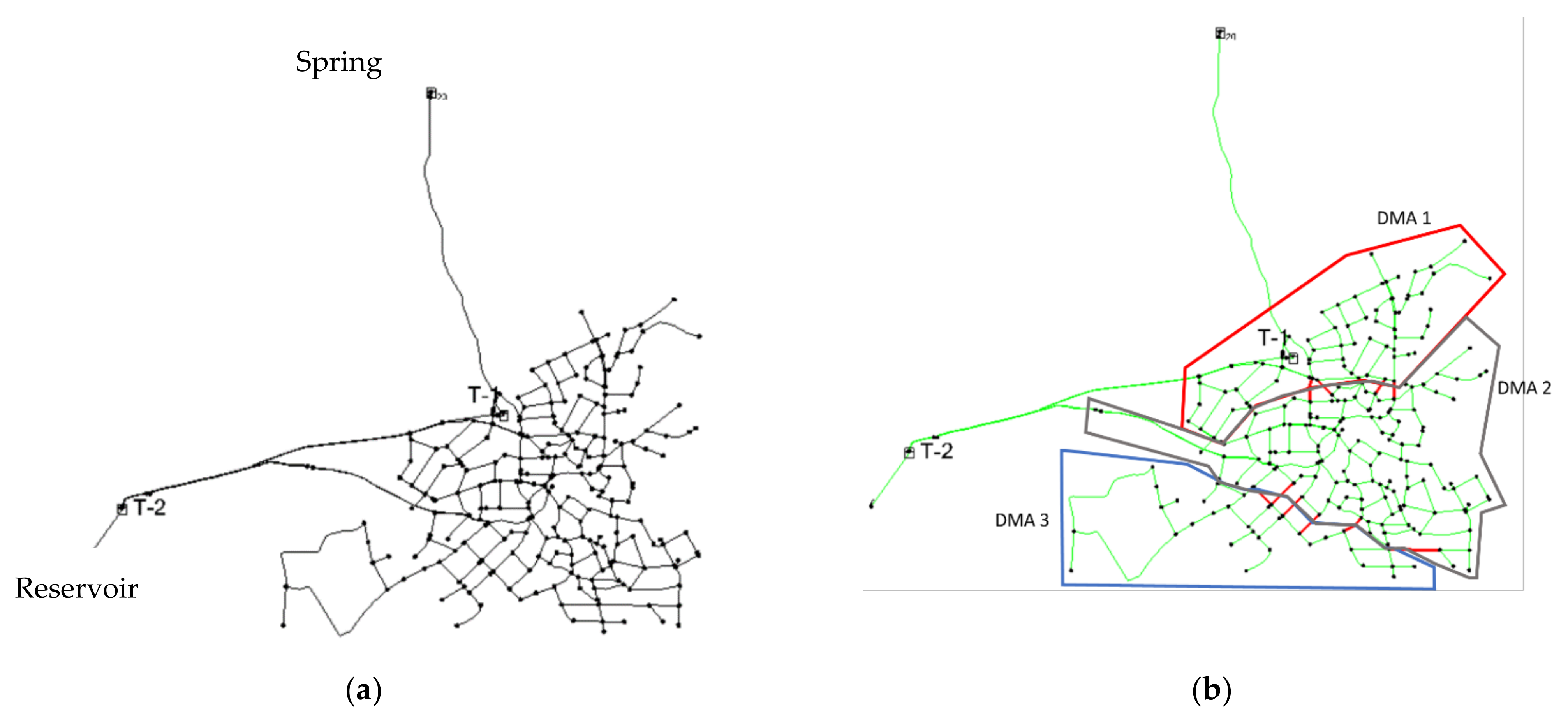
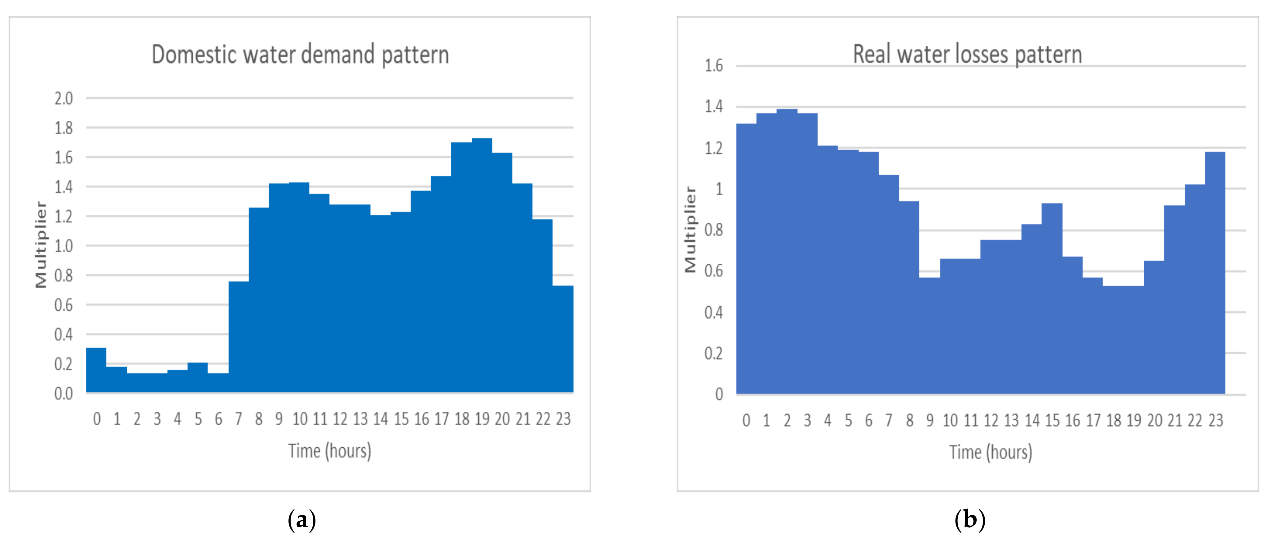
The study area is Eani district in the Kozani municipality in Greece, serving 2006 people. The average water volume entering the network is 1566.96 m³ per day. The system consists of one reservoir, three tanks, 333 pipes of total length of 29,211 m, and 259 pipe junctions (Figure 1). Most of the pipes in the system are polyvinyl chloride (PVC) pipes, and only two pipes of 102 m are made of high-density polyethylene (HDPE). The pipes’ diameters range from 57 to 203.4 mm. The study is based on the digital twin of the water distribution network already developed using Watergems. Domestic water demand follows a 24-h demand pattern, based on the literature (Figure 2a). Non-revenue water components are simulated in the hydraulic model. Specifically, the apparent losses are added to the junctions’ demand proportionally, since their time distribution is similar to the domestic one. However, as real losses’ time distribution is similar to pressure distribution, real losses are allocated in the junctions as a separate demand with its own time pattern, which is inversely proportional to pressure (Figure 2b). To allocate the demand to the network’s junctions, the spatial allocation of water demand at the street level method (SAWDSL) [26] has been adopted. The digital twin has been calibrated and validated.

Water supplied to the network comes from 2 different water sources: (a) water from boreholes (modeled as a reservoir) is stored in tank T-2 and then enters the network with gravity, supplying the high zone and through the tank T-1 the lower zone and (b) water pumped from springs supplies the network through the tank T-1. There is no water treatment, except for chlorination at the entry nodes.

Table 1. Water volume abstracted per water source.

Water Source	Water Volume (m3/Day)	Water Volume (m3/h)
Reservoir	1494.72	62.28
Springs	72.24	3.01
Total	1566.96	65.29

shows the water volume abstracted.

The paper analyzes chlorine residual concentrations in the water distribution system when it is operating as one district metered area (DMA) (scenario A) and when it is divided in three DMAs (scenario B) (Figure 1b). There is a pressure reduction valve (PRV) installed at the inlet point of DMA2, setting pressure to 300 KPa, in scenario B. For each scenario (A and B), conventional and booster chlorination processes are thoroughly analyzed. Conventional chlorination processes refer to the supply of chlorine in the water supply nodes (reservoir and springs), and booster chlorination processes refer to the installation of boosters inline the WDN, as supplementary chlorination devices. Initially, only the water sources are chosen as chlorine inlet/entering points, forming the first five scenarios for different chlorine concentrations. Then, using trial and error, the locations of boosters are chosen, and simulations are made for different chlorine concentrations. The inline chlorination boosters provide chlorination in WDN’s branches and in remote parts/nodes of the network. Watergems is used for the calculation of the chlorine concentration at each pipe and node.

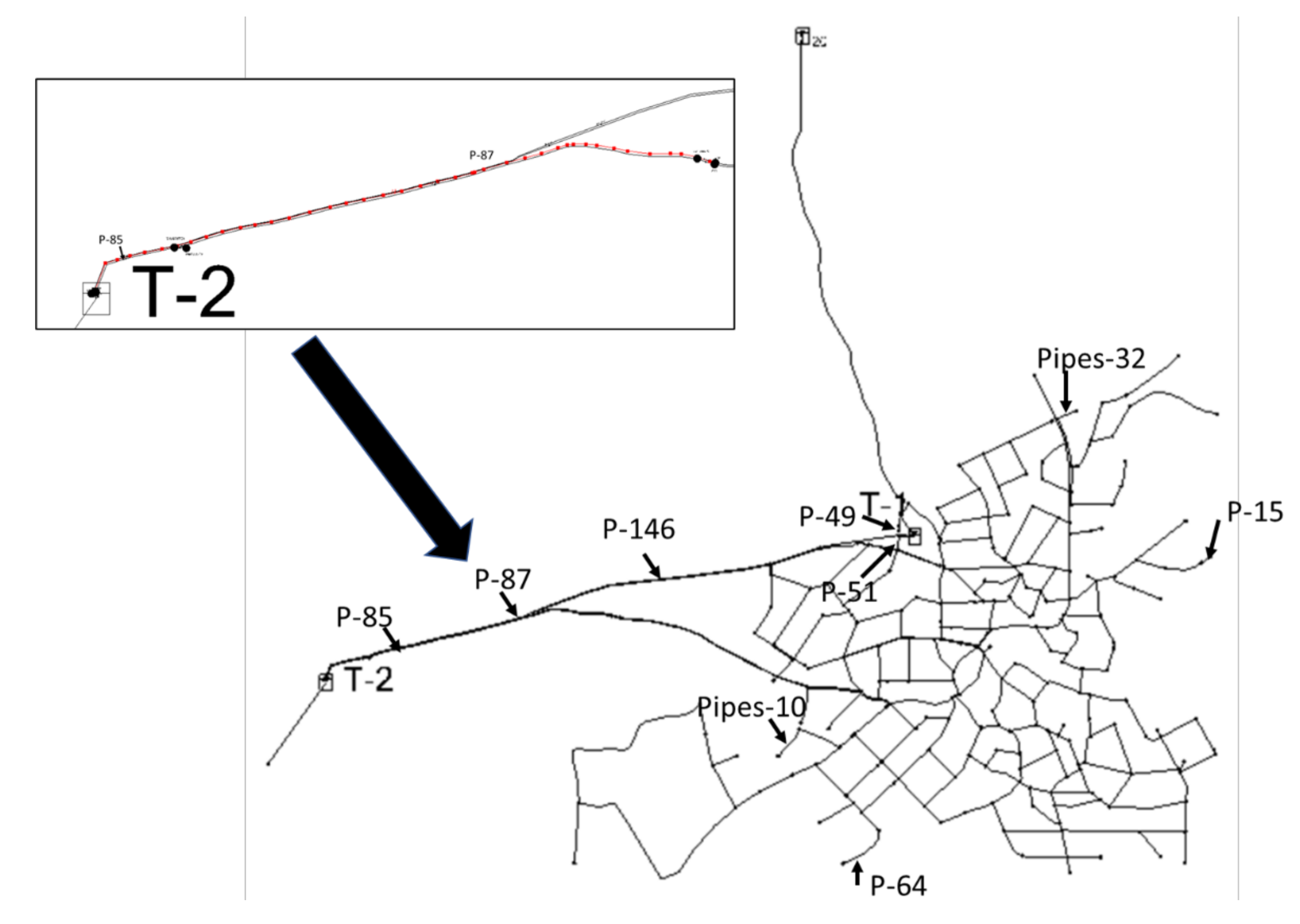
Several nodes and pipes are chosen in the water distribution network to illustrate the chlorine behavior. Nodes and pipes near the water supply sources and nodes and pipes with high water age values are chosen. Pipes P-85, P-87, and P-146 are close to tank T-2, P-49 and P-51 are near tank T-1, and, pipes-10, pipes-32, P-64, and P-15 have increased water age ranging from 20.36 to 63.17 h (scenario A) and from 20.89 to 63.39 h (scenario B) (

Table 2. Pipes and nodes selected for the illustration of chlorine behavior and their water ages (after simulated time of 288 h).

Pipe	Water Age (Hours)		Junctions ID	Water Age (Hours)		Junctions ID	Water Age (Hours)
	Scenario A	Scenario B		Scenario A	Scenario B		Scenario A	Scenario B
P-85	0.95	0.95	J-54	0.95	0.96	Nodes-56	3.98	3.66
P-87	1.34	1.42	J-55	0.95	0.96	Manholes-15	5.37	5.99
P-146	1.71	2.18	J-77	0.95	0.96	J-1	2.86	5.30
P-49	7.90	9.05	J-35	8.18	9.32	J-34	18.41	20.97
P-51	12.34	15.25	J-36	20.36	23.50	J-16	18.59	19.18
Pipes-10	63.17	63.39	Nodes-20	31.15	31.39	Nodes-47	5.17	6.08
P-64	35.07	34.72	J-42	16.86	16.53	Manholes-55	2.35	1.62
Pipes-32	26.73	29.23	Nodes-110	18.25	20.76	495	7.37	7.54
P-15	20.36	20.89	Manholes-87	2.58	1.84	J-7	11.53	13.95
						473	10.61	13.00

and Figure 3). Nodes J-54, J-55, and J-77 are close to tank T-2, nodes J-35 and J-36 are near tank T-1, and nodes J-42, nodes-20, nodes-110, manholes-87, nodes-56, manholes-15, J-1, J-34, J-16, nodes-47, manholes-55, 495, J-7, and 473 are located close to remote parts/nodes of the network experiencing high water ages. Table 2 shows the water ages for the pipes and nodes selected in both scenarios, A and B. The nodes and pipes close to the water sources are chosen as the whole network is fed from these points. It is evident from Table 2 that when the network is divided in DMAs (scenario B), the water age gets higher values.

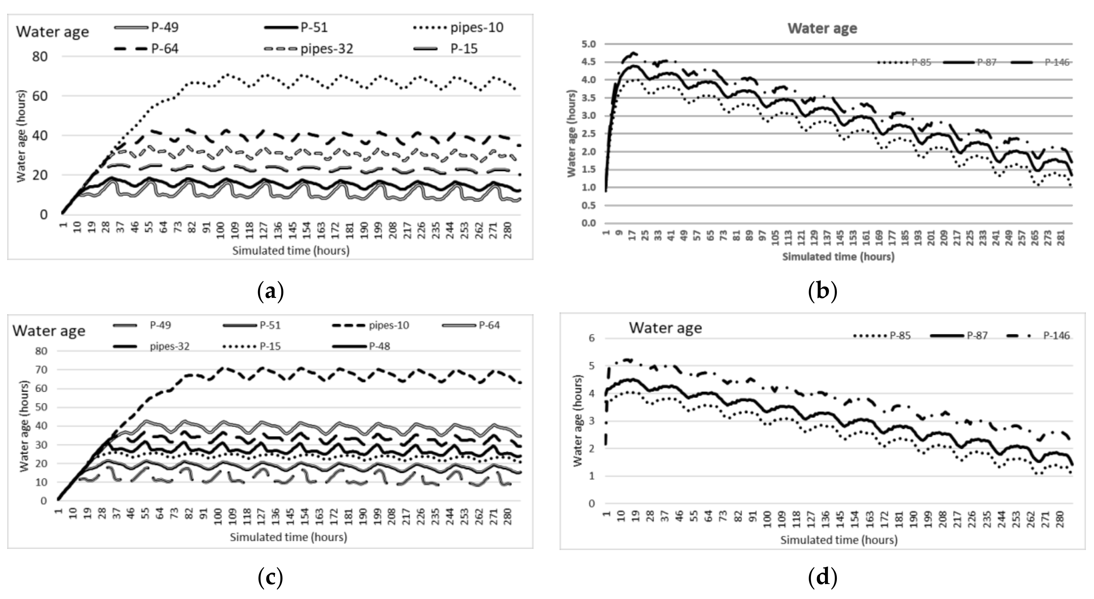
Figure 4a,b show the calculated water age of the pipes over a 288-h period (12 days). Water age values do not vary a lot for pipes P-49, P-51, pipes-10, P-64, pipes-32, and P-15. For pipes P-85, P-87, and P-146, water age values show a downwards trend after having reached their maximum values at about 15–20 h. This is because the initial water age in the tank T-2 is considered to be zero. Then, the tank supplies the network with water, and the water age values are lower. The same trend is evident from Figure 4c,d, except for the initial water age in the tank T-2 considered to be 3.5 h.

4. Results and Discussion

Five conventional chlorination scenarios are analyzed based on different chlorine doses set at the water sources. Chlorination takes place at the nodes where water enters the network. Chlorine concentrations at the reservoir vary from 0.5 to 2.0 mg/L, at a step of 0.5 mg/L, forming the first four scenarios. In the 5th scenario, chlorination takes place both at the reservoir (1 mg/L) and at the springs (0.5 mg/L). The first four scenarios did not take into consideration any chlorination scenario for the springs, as they supply the network only partially. As legislation sets the minimum residual chlorine concentration at the most remote nodes to 0.2 mg/L [4,5], the minimum chlorine dose is set to 0.2 mg/L. The maximum chlorine dose is set to 0.5 mg/L to avoid excess chlorination and disinfection by-products (DBPs) formation and also limit any odor problems. Scenarios 6, 7, and 8 include booster chlorination stations in selected nodes within the water distribution network. For all simulations, the chlorine booster station was modeled as being flow paced to provide constant chlorine concentration for 288 h. As the system needs some time to adjust to a standard behavior, chlorine concentration values are taken at 48 h of simulation.

4.1. Scenario A

As mentioned before, the simulation process includes eight different scenarios. The first five scenarios simulate conventional chlorination taking place in water sources at different concentrations (

Table 3. Chlorine doses (mg/L) applied at booster stations for scenario A.

Selected Junctions (ID)	Chlorine Dose (mg/L)
	Scen.1	Scen.2	Scen.3	Scen.4	Scen.5	Scen.6	Scen.7	Scen.8
Reservoir	0.5	1.0	1.5	2.0	1.0	1.0	0.5	0.5
Springs	0	0	0	0	0.5	1.0	0.5	0.5
manholes-94	0	0	0	0	0	0.6	0.6	0.5
nodes-21	0	0	0	0	0	0.6	0.6	0.5
manholes-4	0	0	0	0	0	0.5	0.5	0.5
manholes-55	0	0	0	0	0	0.5	0.5	0.5
nodes-104	0	0	0	0	0	0.5	0.5	0.5
manholes-11	0	0	0	0	0	0.4	0.4	0.5
460,2	0	0	0	0	0	0.4	0.4	0
482	0	0	0	0	0	0.4	0.4	0.4
manholes-2	0	0	0	0	0	0.3	0.3	0
455,6	0	0	0	0	0	0.3	0.3	0.2
nodes-173	0	0	0	0	0	0.2	0.2	0.2
manholes-35	0	0	0	0	0	0	0	0.5
manholes-25	0	0	0	0	0	0	0	0.3
499,2	0	0	0	0	0	0	0	0.2
nodes-52	0	0	0	0	0	0	0	0.2

). Chlorine is injected at the reservoir at 0.5 mg/L (first scenario). After 288 h of simulation, there are in total 102 pipes with chlorine concentration lower than 0.2 mg/L, not achieving the goal of efficient chlorination. In scenario 2, where a chlorine dose of 1 mg/L is added at the reservoir, 51 pipes have chlorine concentration values higher than 0.5 mg/L, and 11 pipes have chlorine concentration values lower than 0.2 mg/L. When the chlorine concentration added at the reservoir is 1.5 mg/L (scenario 3), only two pipes (P-64 and pipes-10) have chlorine concentration lower than 0.2 mg/L, while 224 pipes have chlorine concentration values higher than 0.5 mg/L. There is no pipe with residual chlorine lower than 0.2 mg/L (effective chlorination is achieved) when the chlorine dose added at the reservoir is 2 mg/L (scenario 4). However, in this scenario, 245 pipes have chlorine concentration values higher than 0.5 mg/L. In the fifth scenario, the chlorine dose added at the reservoir is 1 mg/L, and the dose added at the springs is 0.5 mg/L. Chlorine concentration is higher than 0.5 mg/L in 107 pipes, and 12 pipes have chlorine concentration lower than 0.2 mg/L, showing that scenario 5 gives worse results from scenario 2 (1 mg/L added at the reservoir).

In order to achieve efficient chlorination within the limits set by the legislation and the desired maximum limit of 0.5 mg/L, eleven chlorination boosters are added in the network. The boosters’ locations are preferably upstream of the network’s branches. Trial and error took place to finally select the boosters’ installation nodes (Table 3). The nodes selected supply branches of the network with water to allow for the adequate contact time (for example nodes-173, manholes-4, 455,6, manholes-11, etc.). When chlorination is not efficient (values lower of 0.2 mg/L) at all the network’s nodes and pipes, then additional boosters are located at the remote parts/nodes of the network (for example, manholes-55). Initially, the applied chlorination doses in the boosters are set to 0.5 mg/L. After several trial-and-error simulations, the chlorine concentration for each booster chlorination is determined in order to achieve effective chlorination (residual chlorine concentration >0.2 mg/L) at all pipes in the WDN (scenario 6). In this scenario, the chlorine dose added at the reservoir is 1 mg/L and at the spring the dose is 1 mg/L. Eleven boosters are set at specific nodes in the water distribution network with applied chlorination doses varying from 0.2 to 0.5 mg/L (Table 3). The goal is to achieve a detectable chlorine residual of 0.2 mg/L at remote parts/nodes in the WDN. The results showed that although all pipes have detectable chlorine concentrations of a minimum of 0.2 mg/L, there are 54 pipes with chlorine concentration values higher than 0.5 mg/L. In order to avoid chlorine concentrations higher than 0.5 mg/L, scenario 7 was set up. In this scenario, the chlorine doses added at the reservoir and at the springs are 0.5 mg/L. The chlorine doses at the 11 selected boosters range from 0.2 to 0.6 mg/L. In order to arrive at the lowest possible chlorine concentrations at the boosters, trial-and-error took place. The concentration of 0.6 mg/L could not be avoided. Although efficient chlorination is achieved at all pipes in scenario 7, there are still some remote nodes where residual chlorine is less than 0.2 mg/L. Therefore, it was necessary to add two additional chlorine boosters and move another two boosters to other nodes, while the proper chlorine concentration injected is achieved after several trial-and-error attempts (Table 3).

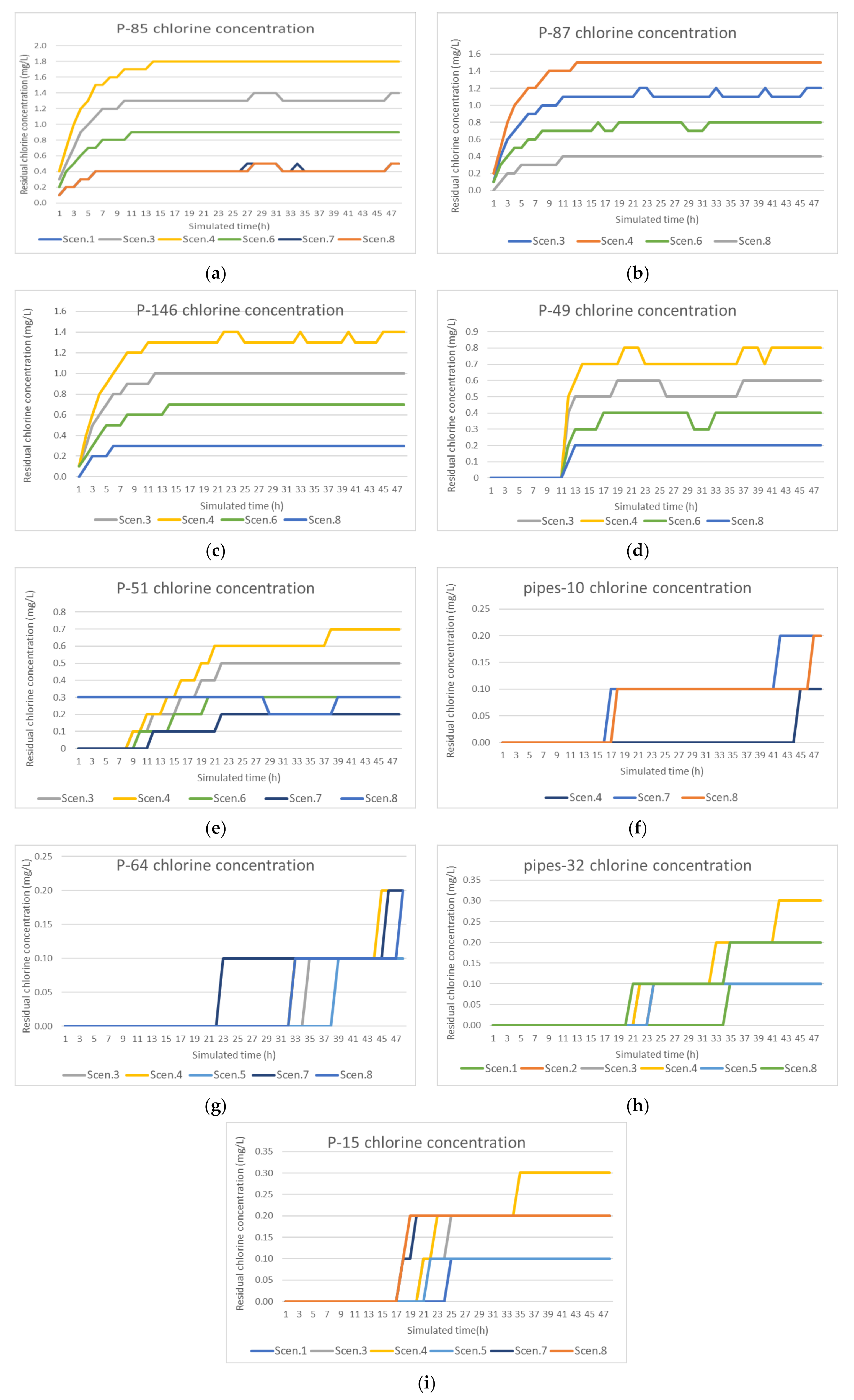
Scenarios 4–8 ensure detectable limits of residual chlorine concentration (>0.2 mg/L) at the selected points after 48 h. However, in scenarios 4 and 6, there are pipes with chlorine concentration exceeding 0.5 mg/L. Figure 5a–i show the chlorine residual concentration variations at the eight selected pipes within the first 48 h. For pipe P-85, which is near the reservoir supplying the whole network with water, the chlorine residual values range from 0.5 (scenarios 1, 7, and 8) to 1.8 mg/L (scenario 4). After two hours, the chlorine concentration already achieved the threshold of 0.2 mg/L in scenarios 7 and 8. For pipe P-87, which is also near the reservoir, chlorine residual values range from 0.4 (scenarios 1, 7, and 8) to 1.5 mg/L (scenario 4). Chlorine residual values range from 0.3 (scenarios 1, 7, and 8) to 1.4 mg/L (scenario 4) for pipe P-146 (a long pipe near the reservoir supplying a big part of the network with water). Chlorine concentration achieved the value of 0.2 mg/L within the first two hours for both pipes P-87 and P-146. For P-49, a pipe near tank T-1, the chlorine residual values range from 0.2 (scenarios 1, 7, and 8) to 0.8 mg/L (scenario 4). Almost in all scenarios, the time to achieve detectable chlorine concentration values is 12–13 h. Almost the same stands for pipe P-51 (located close to tank T-1), where residual chlorine values range from 0.2 (scenarios 1 and 7) to 0.7 mg/L (scenario 4). In scenario 8, the residual chlorine concentration value is 0.3 mg/L after one hour of simulation. It is evident that remote pipes receive effective chlorination after a long time period ranging from 17 h (pipes-10) to 46 h (P-64). Pipes-10 (remote pipe in the network) does not get detectable chlorine concentrations in scenarios 1–5 within 48 h. Chlorine concentration values of 0.2 mg/L are achieved in scenario 6 and 7 after 42 h and in scenario 8 after 46 h. Chlorine residual values range from 0 (scenario 1) to 0.2 mg/L (scenarios 4, 6, 7, and 8) for P-64, achieving effective chlorination after 46 h in scenarios 4, 6, and 7. In pipes-32, another remote pipe, chlorine concentrations range from 0.1 (scenarios 1, 2, 5) to 0.3 mg/L (scenario 4). The desired value of 0.2 mg/L chlorine residual is achieved after 35 h in scenarios 7 and 8. Finally, in pipe P-15 (also remote pipe), residual chlorine concentration ranges from 0.1 (scenarios 1, 2, 5) to 0.3 mg/L (scenario 4). The time to achieve the detectable concentration of 0.2 mg/L in scenario 8 is 17 h. It can be concluded that the remote pipes in the network need boosters to achieve the efficient chlorination concentration of 0.2 mg/L (Figure 5).

Table 4. Chlorine residual concentrations (mg/L) at selected pipes and nodes for scenario A.

Pipe ID	Chlorine Residual Concentration (mg/L)
	Scen.1	Scen.2	Scen.3	Scen.4	Scen.5	Scen.6	Scen.7	Scen.8
P-85	0.5	0.9	1.4	1.8	0.9	0.9	0.5	0.5
P-87	0.4	0.8	1.2	1.5	0.8	0.8	0.4	0.4
P-146	0.3	0.7	1.0	1.4	0.7	0.7	0.3	0.3
P-49	0.2	0.4	0.6	0.8	0.4	0.4	0.2	0.2
P-51	0.2	0.3	0.5	0.7	0.3	0.3	0.2	0.3
pipes-10	0.0	0.0	0.0	0.1	0.0	0.2	0.2	0.2
P-64	0.0	0.1	0.1	0.2	0.1	0.2	0.2	0.2
pipes-32	0.1	0.1	0.2	0.3	0.1	0.2	0.2	0.2
P-15	0.1	0.1	0.2	0.3	0.1	0.2	0.2	0.2
Junctions ID
J-54	0.5	0.9	1.4	1.8	0.9	0.9	0.5	0.5
J-55	0.4	0.9	1.3	1.8	0.9	0.9	0.4	0.4
J-77	0.4	0.9	1.3	1.8	0.9	0.9	0.4	0.4
J-35	0.2	0.4	0.6	0.7	0.4	0.4	0.2	0.2
J-36	0.1	0.3	0.4	0.6	0.3	0.3	0.2	0.2
Nodes-20	0.1	0.1	0.2	0.3	0.1	0.4	0.4	0.4
J-42	0.1	0.2	0.3	0.3	0.3	0.3	0.3	0.3
Nodes-110	0.1	0.2	0.3	0.4	0.2	0.2	0.2	0.2
Manholes-87	0.3	0.6	0.9	1.2	0.6	0.6	0.5	0.5
Nodes-56	0.2	0.3	0.5	0.7	0.3	0.6	0.6	0.5
Manholes-15	0.2	0.3	0.5	0.6	0.3	0.3	0.3	0.4
J-1	0.3	0.6	0.9	1.1	0.6	0.6	0.3	0.3
J-34	0.1	0.3	0.4	0.5	0.3	0.3	0.2	0.2
J-16	0.1	0.2	0.2	0.3	0.2	0.2	0.2	0.2
Nodes-47	0.1	0.2	0.3	0.4	0.2	0.2	0.2	0.3
Manholes-55	0.3	0.6	0.9	1.2	0.6	0.6	0.5	0.5
495	0.1	0.2	0.3	0.4	0.2	0.3	0.3	0.3
J-7	0.1	0.2	0.3	0.4	0.2	0.3	0.3	0.3
473	0.1	0.2	0.3	0.5	0.2	0.3	0.3	0.3
Total chlorine dose (g/day)	747.4	1494.7	2242.1	2989.4	1495.1	1522.7	779.7	777.0
Safe water volume (%)	73.06	93.78	46.16	22.06	93.82	93.22	97.98	100.00
Min chlorine concentration at 48 h (mg/L)	0.0	0.0	0.0	0.0	0.0	0.1	0.1	0.2
Max chlorine concentration at 48 h (mg/L)	0.5	0.9	1.4	1.8	0.9	0.9	0.6	0.5
Mean chlorine concentration at 48 h (mg/L)	0.18	0.36	0.54	0.72	0.36	0.39	0.27	0.27

presents the values of chlorine residual after 48 h in the selected pipes and nodes.

In order to assess the effectiveness of the chlorination scenarios, the total chlorine dose (g/day), the percentage of safe water (with chlorine concentration within the limits), and minimum, maximum, and average chlorine concentrations to all nodes at 48 h are estimated (Table 4). Chlorine mass takes its lowest value in scenario 8, compared to scenarios achieving effective chlorination. The maximum water volume with residual chlorine concentrations within the limits (100%) is achieved in scenario 8.

4.2. Scenario B

Eight chlorination scenarios comprise scenario B. The conditions are the same as in scenario A for the first five scenarios. For scenarios 6–8, the same methodology as before is followed. Boosters are located in different nodes in scenario B, as there are three DMAs in the WDN (

Table 5. Chlorine doses (mg/L) applied at booster stations for scenario B.

Selected Junctions ID	Chlorine Dose (mg/L)
	Scen.1	Scen.2	Scen.3	Scen.4	Scen.5	Scen.6	Scen.7	Scen.8
Reservoir	0.5	1.0	1.5	2.0	1.0	1.0	0.5	0.5
Springs	0	0	0	0	0.5	1.0	0.6	0.5
Manholes-3	0	0	0	0	0	0.5	0.5	0.5
Manholes-55	0	0	0	0	0	0.5	0.5	0.5
Manholes-94	0	0	0	0	0	0.5	0.5	0.5
Nodes-21	0	0	0	0	0	0.5	0.5	0.5
Manholes-4	0	0	0	0	0	0.5	0.4	0.4
Manholes-11	0	0	0	0	0	0.5	0.4	0.5
Manholes-7	0	0	0	0	0	0.5	0.4	0.5
481,5	0	0	0	0	0	0.5	0.4	0.4
Manholes-57	0	0	0	0	0	0.5	0.3	0.4
482,2	0	0	0	0	0	0.5	0.2	0.3
Manholes-38	0	0	0	0	0	0	0	0.4
473,5	0	0	0	0	0	0	0	0.3

). When the chlorine dose is 0.5 mg/L (scenario 1), there are 127 pipes where chlorine concentration after 288 h is lower than 0.2 mg/L. When chlorine concentration added at the reservoir is 1 mg/L (scenario 2), 41 pipes have chlorine concentration values higher than 0.5 mg/L, and 21 pipes have chlorine concentration values lower than 0.2 mg/L. In scenario 3 (1.5 mg/L chlorine dose added at the reservoir), chlorine residual lower than 0.2 mg/L is achieved in six pipes, while 134 pipes have chlorine concentration values higher than 0.5 mg/L. When the chlorine dose added at the reservoir is 2 mg/L (scenario 4), only two pipes (pipes-10 and pipes-115) do not achieve effective chlorination, while 208 pipes have chlorine concentrations higher than 0.5 mg/L. When the chlorine dose added at the reservoir is 1 mg/L and the chlorine dose added at the springs is 0.5 mg/L (scenario 5), chlorine residual higher than 0.5 mg/L is found in 41 pipes, and 22 pipes do not achieve effective chlorination. The results of scenario 5 are almost the same ones as those of scenario 2 (1 mg/L added in the reservoir).

Ten boosters are installed in the WDN forming scenarios 6 and 7. The boosters’ locations selected are based on the results of the first five scenarios and several trial-and-error simulations. The nodes selected for the boosters’ installation are upstream of the network’s branches (e.g., manholes-3, 481,5, etc.) and close to remote nodes with high water age (e.g., manholes-11). The goal is to achieve effective chlorination at all pipes in the WDN. The chlorine dose added in scenario 6 is set to 1 mg/L at the reservoir and the springs and 0.5 mg/L at the boosters (Table 5). Although all pipes have detectable chlorine concentrations of a minimum of 0.2 mg/L, there are 41 pipes with chlorine concentration values higher than 0.5 mg/L. This resulted in scenario 7, where the chlorine dose added in the reservoir is 0.5 mg/L, and in the springs, it is 0.6 mg/L. The chlorine doses at the ten boosters range from 0.2 to 0.5 mg/L. However, eight remote nodes have chlorine concentration lower than 0.2 mg/L. Thus, two more chlorination boosters are added, and chlorine doses injected are set within the limits of 0.2 to 0.5 mg/L.

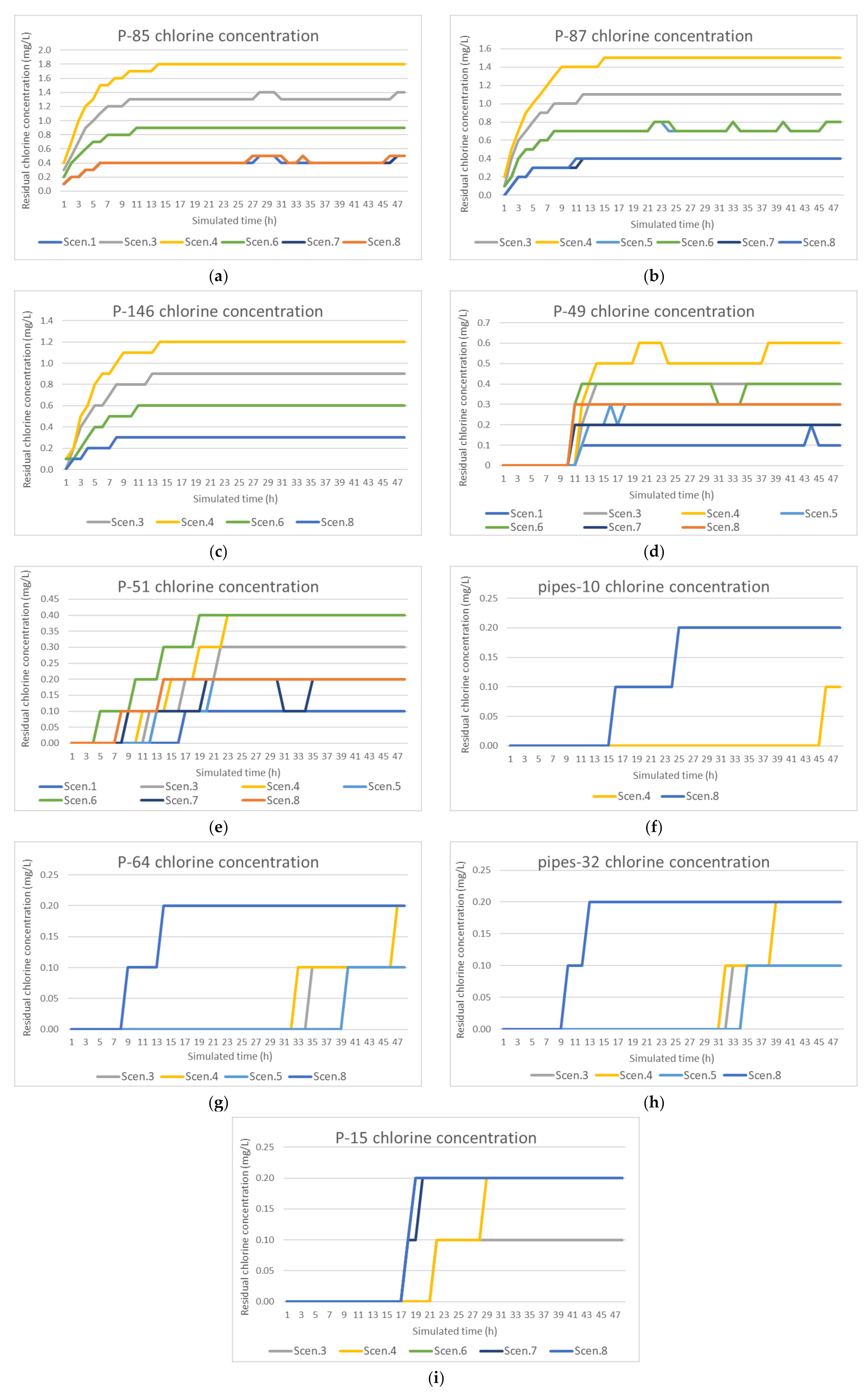
Scenarios 6–8 ensure detectable limits of residual chlorine concentration (>0.2 mg/L) at the selected points after 48 h. However, in scenario 6, there are pipes where chlorine concentration exceeds 0.5 mg/L. Figure 6a–i show the chlorine residual concentration variations at the nine selected pipes within the first 48 h. The pipes near tank T-2 achieve effective chlorination in the 2nd hour of operation (P-85), after 3 h (P-87), and after 4 h (P-146). Chlorine residual values range from 0.5 (scenarios 1, 7, and 8) to 1.8 mg/L (scenario 4) for P-85 and from 0.4 (scenarios 1, 7, and 8) to 1.5 mg/L (scenario 4) for P-87. The residual chlorine concentration for the P-146 ranges from 0.3 (scenarios 1, 7, and 8) to 1.2 mg/L (scenario 4). The time to achieve effective chlorination for the pipes close to tank T-1 is 10 h for P-49 and 13 h for P-51 (scenario 8). In all other scenarios, this concentration is achieved after higher time values for P-49 but earlier for scenario 6 for P-51. For P-49 and P-51, residual chlorine concentrations range from 0.1 (scenario 1) to 0.6 mg/L (scenario 4) and from 0.1 (scenario 1) to 0.4 mg/L (scenarios 4 and 6), respectively. For pipes located at remote parts of the network, the effective chlorine concentration is achieved after 24 h (pipes-10), after 13 h (P-64), after 12 h (pipes-32), and after 18 h (P-15). For pipes-10, effective chlorine concentration is only achieved in scenarios 6, 7, and 8. In all other scenarios, chlorine concentration is zero or below 0.2 mg/L. P-64 achieves effective chlorination only in scenarios 4, 6, 7, and 8. At pipes-32, the residual chlorine concentration ranges from 0.1 (scenarios 2, 3, and 5) to 0.2 mg/L (scenarios 4, 6, 7, and 8), while in scenario 1, the residual chlorine concentration is zero. The same stands for P-15. Scenario B verifies that the remote pipes in the network need boosters to achieve the efficient chlorination concentration of 0.2 mg/L.

Table 6. Chlorine residual concentrations at selected pipes and nodes for scenario B.

Pipe ID	Residual Chlorine Concentration (mg/L)
	Scen.1	Scen.2	Scen.3	Scen.4	Scen.5	Scen.6	Scen.7	Scen.8
P-85	0.5	0.9	1.4	1.8	0.9	0.9	0.5	0.5
P-87	0.4	0.8	1.1	1.5	0.8	0.8	0.4	0.5
P-146	0.3	0.6	0.9	1.2	0.6	0.6	0.3	0.3
P-49	0.1	0.3	0.4	0.6	0.3	0.4	0.2	0.3
P-51	0.1	0.2	0.3	0.4	0.2	0.4	0.2	0.2
Pipes-10	0.0	0.0	0.0	0.1	0.0	0.2	0.2	0.2
P-64	0.0	0.1	0.1	0.2	0.1	0.2	0.2	0.2
Pipes-32	0.0	0.1	0.1	0.2	0.1	0.2	0.2	0.2
P-15	0.0	0.1	0.1	0.2	0.1	0.2	0.2	0.2
Junctions ID
J-54	0.5	0.9	1.4	1.8	0.9	0.9	0.5	0.5
J-55	0.4	0.9	1.3	1.8	0.9	0.9	0.4	0.4
J-77	0.4	0.9	1.3	1.8	0.9	0.9	0.4	0.4
J-35	0.1	0.3	0.4	0.6	0.3	0.4	0.2	0.3
J-36	0.1	0.2	0.3	0.4	0.2	0.3	0.2	0.2
Nodes-20	0.1	0.	0.2	0.2	0.1	0.3	0.3	0.3
J-42	0.1	0.2	0.2	0.3	0.2	0.3	0.3	0.3
Nodes-110	0.1	0.1	0.2	0.3	0.1	0.2	0.2	0.2
Manholes-87	0.3	0.7	1.0	1.4	0.7	0.7	0.5	0.5
Nodes-56	0.2	0.3	0.5	0.6	0.3	0.5	0.5	0.5
Manholes-15	0.1	0.2	0.3	0.4	0.2	0.4	0.3	0.4
J-1	0.2	0.4	0.6	0.8	0.4	0.4	0.2	0.2
J-34	0.1	0.2	0.3	0.3	0.2	0.3	0.2	0.2
J-16	0.1	0.1	0.1	0.2	0.1	0.2	0.2	0.2
Nodes-47	0.1	0.1	0.2	0.3	0.1	0.2	0.2	0.2
Manholes-55	0.4	0.7	1.1	1.5	0.7	0.7	0.5	0.5
495	0.1	0.2	0.3	0.4	0.2	0.3	0.3	0.3
J-7	0.1	0.1	0.2	0.3	0.1	0.2	0.2	0.3
473	0.1	0.2	0.2	0.3	0.2	0.2	0.2	0.3
Total chlorine dose (g/day)	747.4	1494.7	2242.1	2989.4	1495.1	1516.5	770.4	775.5
Safe water volume (%)	69.23	85.58	52.70	24.59	85.61	90.43	98.89	100.00
Min chlorine concentration at 48 h (mg/L)	0.0	0.0	0.0	0.0	0.0	0.1	0.1	0.2
Max chlorine concentration at 48 h (mg/L)	0.5	0.9	1.4	1.8	0.9	0.9	0.5	0.5
Mean chlorine concentration at 48 h (mg/L)	0.16	0.33	0.49	0.66	0.33	0.38	0.27	0.29

shows the values of chlorine residual after 48 h at selected pipes and nodes and the total chlorine dose (g/day). The total chlorine dose is significantly reduced in scenario 8, confirming the findings from other studies that when using chlorination boosters, total chlorine mass is reduced. Table 6 presents the total chlorine mass, the percentage of safe water (with chlorine concentrations between the limits set), minimum, maximum, and average chlorine concentrations in all nodes at 48 h. The percentage of safe water is 100% in scenario 8.

4.3. Results from the Comparison of Scenarios A and B

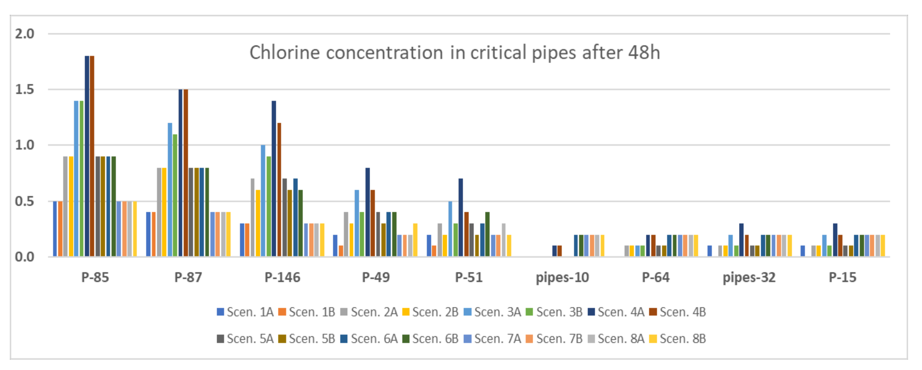
The comparison of the results from scenario A and scenario B shows that water age values are higher for the critical pipes in scenario B. This is an expected result, as the DMAs formation and PRV installation lead to higher water age values. The average water pressure in the whole WDN in scenario A is 779 KPa, while in scenario B, it is reduced to 526 KPa (reduction 32.5%). Comparing the residual chlorine concentration at the critical pipes for all scenarios after 48 h of operation shows that chlorine concentration is higher in scenario A for many pipes (Figure 7). Specifically, for P-146, the chlorine concentration is higher in all scenarios when there are no DMAs, except for scenarios 1, 7, and 8, where the concentrations are equal. For pipe P-49, chlorine concentration is higher in all scenarios without DMAs, except for scenarios 6 and 7 where the concentrations are equal, and scenario 8, where chlorine concentration is higher in scenario B. For P-51, the chlorine concentrations are equal in scenario 7, regardless of the DMAs’ existence. For pipes P-15 and pipes-32, the chlorine concentration is higher in scenarios 3 and 4 without DMAs. For these pipes in all other scenarios, the concentration is equal except for scenario 1 where the concentration is zero when there are DMAs. Finally, for pipe P-87, the chlorine concentration is equal in all scenarios except for scenario 3, where the concentration is higher without DMAs. Thus, when there are DMAs formed in a WDN, the time for effective chlorination is higher in critical pipes.

4.4. Discussion

The analysis revealed that there are remote network pipes and nodes that experience high water age. To achieve effective chlorination at these pipes and nodes with safe water volume more than 90%, the chlorine dose at the water supply nodes must be high (e.g., scenario 5A), resulting in excess chlorine concentrations near the chlorine injection nodes and insufficient chlorination in some remote nodes. Several research studies have shown the importance of using additional inline chlorination boosters [7,8,9,10,11,12,13,14,15,16,17] to ensure more uniform residual chlorine concentrations throughout the network. This conclusion agrees with the findings of this study. At the same time, booster chlorination prevents the formation of DBPs in water as chlorine concentrations are low. As it is accepted that there is a linear relationship between THMs’ formation and chlorine consumption (40 μg THMs are formed for 1 mg chlorine consumed); it is important to inject low chlorine concentrations, safeguarding efficient chlorination [21]. In this study, the maximum chlorine dose injected is 0.5 mg/L, and using trial-and-error, the chlorine dose in each node (with booster) is set between 0.2 and 0.5 mg/L. Based on the theoretic approach, the THMs concentration is not high. As the water in this WDN comes from groundwater and springs, organic matter concentrations are low. Water origin and its initial quality condition is important to plan disinfection strategies [27]. THMs’ formation due to reactions with the pipe wall and at the bulk phase is complex, requiring onsite samplings and chemical analyses. In the literature, there are studies using various multivariate statistical techniques such as multiple regression analysis to develop THMs’ formation models based on time series of other water quality parameters [1]. Such techniques are also used for water quality assessment and pollution source identification [28].

DMAs’ formation is accepted as a good way to manage water distribution networks more efficiently and at the same time apply pressure management measures to reduce water losses. However, the formation of DMAs and the reduction of pressure result in higher water age values and possible contamination phenomena. Due to high water age values, it is expected that chlorination needs more time and higher chlorine doses to achieve efficient disinfection. The results of this study showed that the formation of three DMAs and the installation of a PRV reduced the average operating pressure by 32.5%. The average water age is increased by 8.27% (the average water age in scenario A is 8.16 h and in scenario B is 8.83 h). Although to achieve efficient chlorination takes more time when DMAs exist, the delay to achieve the minimum residual chlorine concentration is not proportional. For example, the residual chlorine concentration in pipe P-146 (located near the reservoir) obtains the value of 0.2 mg/L in three hours in scenario A and in four hours in scenario B. Of course, it depends on the location of the chlorination point in relation to the location of the pipe. However, the benefits of DMAs formation and application of pressure management are significant [2,3], and they do not affect chlorination drastically. Thus, it is important to include water age and residual chlorine as criteria in pressure optimization attempts and DMAs’ formation. The results from this study are based on simulations. To validate the results, onsite measurements are needed. Continuous measurement and validations are necessary especially for chlorine decay and THMs formation, as they are also affected by other factors.

It is well known that there are water quality parameters affecting disinfection efficiency. These parameters are turbidity, pH, temperature, and organic compounds. Chlorine reacts with compounds found in water. However, the present study does not analyze how chlorine will impact other physicochemical parameters. To study the effects of chlorine, water samplings and analyses should take place in future research.

5. Conclusions

The primary aim of the present study is to address (a) the impact of boosters’ chlorination on critical pipes in a WDN and (b) the impact of DMAs’ formation on critical pipes’ chlorination. A thorough analysis took place, including several chlorination scenarios, where chlorine is injected only at water sources or both at water sources and inline using chlorination boosters. The impact of chlorination boosters and DMAs is studied in critical pipes selected in the WDN. These pipes are located near the water sources and at remote parts in the network with high water age values. The model simulations revealed that the use of additional chlorination boosters provide a more uniform chlorination throughout the WDN, achieving effective chlorination of 0.2 mg/L without exceeding the maximum value of 0.5 mg/L, avoiding the formation of DBPs. The use of additional inline chlorination boosters allows for more effective chlorination compared to conventional chlorination taking place at the water sources of the network. Using chlorination boosters, there is a significant reduction of total chlorine dose compared to conventional chlorination. The formation of DMAs (and installation of PRVs) showed that although the operating pressure is lower and the WDN does not suffer from high water losses, water age values are increased, especially in remote pipes of the network. This fact results in delayed chlorination exposing the system to pathogens. However, the excess time needed for effective chlorination is not proportional to reduced pressure. Therefore, when water operators make decisions to improve the network’s performance level (such as DMAs’ formation and pressure reduction), it is important to achieve the proper balance between water pressure and effective chlorination. When water utilities want to optimize their water pressure, they should use residual chlorine as an additional criterion in optimization. Water utility managers should not underestimate both water age and residual chlorine during the decision-making process to reduce water losses, as water quality is important for consumers’ health.

References

- Tsitsifli, S.; Kanakoudis, V. Developing THMs’ Predictive Models in Two Water Supply Systems in Greece. Water 2020, 12, 1422. [Google Scholar] [CrossRef]
- Kanakoudis, V.; Muhammetoglu, H. Urban Water Pipe Networks Management Towards Non-Revenue Water Reduction: Two Case Studies from Greece and Turkey. Clean-Soil Air Water 2013, 42, 880–892. [Google Scholar] [CrossRef]
- Ciaponi, C.; Creaco, E.; Di Nardo, A.; Di Natale, M.; Giudicianni, C.; Musmarra, D.; Santonastaso, G.F. Reducing impacts of contamination in water distribution networks: A combined strategy based on network partitioning and installation of water quality sensors. Water 2019, 11, 1315. [Google Scholar] [CrossRef] [Green Version]
- World Health Organization. Guidelines for Drinking-Water Quality, 4th ed.; WHO: Geneva, Switzerland, 2017. [Google Scholar]
- Joint Ministerial Decision, No.67322/6.9.2017 on “Quality of Water Intended for Human Consumption in Compliance with the Directive 98/83/EC of the European Council of 3rd November 1998 as Amended by the Directive 2015/1787 (L260, 7.10.2015)”. (in Greek). Available online: https://elinyae.gr/sites/default/files/2019-07/3282b_2017.1528374178932.pdf (accessed on 11 January 2021).
- Directive (EU) 2020/2184 of the European Parliament and of the Council of 16 December 2020 on the Quality of Water Intended for Human Consumption. Available online: https://eur-lex.europa.eu/eli/dir/2020/2184/oj (accessed on 11 January 2021).
- Tryby, M.E.; Boccelli, D.L.; Koechling, M.T.; Uber, J.G.; Summers, R.S.; Rossman, L.A. Booster chlorination for managing disinfectant residuals. J. Am. Water Works Assoc. 1999, 91, 95–108. [Google Scholar] [CrossRef]
- Boccelli, D.L.; Tryby, M.E.; Uber, J.G.; Rossman, L.A.; Zierolf, M.L.; Polycarpou, M.M. Optimal scheduling of booster disinfection in water distribution systems. J. Water Resour. Plan. Manag. 1998, 124, 99–111. [Google Scholar] [CrossRef]
- Munavalli, G.R.; Kumar, M.M. Optimal scheduling of multiple chlorine sources in water distribution systems. J. Water Resour. Plan. Manag. 2003, 129, 493–504. [Google Scholar] [CrossRef]
- Tryby, M.E.; Boccelli, D.L.; Uber, J.G.; Rossman, L.A. Facility location model for booster disinfection of water supply networks. J. Water Resour. Plan. Manag. 2002, 128, 322–333. [Google Scholar] [CrossRef]
- Propato, M.; Uber, J.G. Linear least-squares formulation for operation of booster disinfection systems. J. Water Resour. Plan. Manag. 2003, 130, 53–62. [Google Scholar] [CrossRef]
- Yoo, D.G.; Lee, S.M.; Lee, H.M.; Choi, Y.H.; Kim, J.H. Optimizing Re-Chlorination Injection Points for Water Supply Networks Using Harmony Search Algorithm. Water 2018, 10, 547. [Google Scholar] [CrossRef] [Green Version]
- Prasad, T.D.; Walters, G.A.; Savic, D.A. Booster disinfection of water supply networks: Multiobjective approach. J. Water Resour. Plan. Manag. 2004, 130, 367–376. [Google Scholar] [CrossRef]
- Ostfeld, A.; Salomons, E. Conjunctive optimal scheduling of pumping and booster chlorine injections in water distribution systems. Eng. Optim. 2006, 38, 337–352. [Google Scholar] [CrossRef]
- Seyoum, A.G.; Tanyimboh, T.T. Integration of hydraulic and water quality modelling in distribution networks: EPANET-PMX. Water Resour. Manag. 2017, 31, 4485–4503. [Google Scholar] [CrossRef] [Green Version]
- Seyoum, A.G.; Tanyimboh, T.T.; Siew, C. Assessment of water quality modelling capabilities of EPANET multiple species and pressure-dependent extension models. Water Sci. Technol. Water Supply 2013, 13, 1161–1166. [Google Scholar] [CrossRef] [Green Version]
- Lee, S.M.; Lee, H.M.; Yoo, D.G.; Kim, J.H. A comparative study on a hydraulic and water-quality analysis method for determining rechlorination injection points for a water-supply network. Water 2019, 11, 697. [Google Scholar] [CrossRef] [Green Version]
- Chatzivasili, S.; Papadimitriou, K.; Kanakoudis, V. Optimizing the Formation of DMAs in a Water Distribution Network through Advanced Modelling. Water 2019, 11, 278. [Google Scholar] [CrossRef] [Green Version]
- Chatzivasili, S.; Papadimitriou, K.; Kanakoudis, V.; Patelis, M. Optimizing the Formation of DMAs in a Water Distribution Network Applying Geometric Partitioning (GP) and Gaussian Mixture Models (GMMs). Proceedings 2018, 2, 601. [Google Scholar] [CrossRef] [Green Version]
- Kourbasis, N.; Patelis, M.; Tsitsifli, S.; Kanakoudis, V. Optimizing water age and pressure in drinking water distribution networks. Environ. Sci. Proc. 2020, 2, 51. [Google Scholar] [CrossRef]
- Carrico, B.; Singer, P.C. Impact of booster chlorination on chlorine decay and THM production: Simulated analysis. J. Environ. Eng. 2009, 135, 928–935. [Google Scholar] [CrossRef]
- Vasconcelos, J.J.; Rossman, L.A.; Grayman, W.M.; Boulos, P.F.; Clark, R.M. Kinetics of chlorine decay. J. AWWA 1997, 89, 54–65. [Google Scholar] [CrossRef]
- Rossman, L.A.; Brown, R.A.; Singer, P.C.; Nuckols, J.R. DBP formation kinetics in a simulated distribution system. Water Res. 2001, 35, 3483–3489. [Google Scholar] [CrossRef]
- Blokker, M.; Vreeburg, J.; Speight, V. Residual chlorine in the extremities of the drinking water distribution system: The influence of stochastic water demands. Procedia Eng. 2014, 70, 172–180. [Google Scholar] [CrossRef] [Green Version]
- Rossman, L.A.; Clark, R.M.; Grayman, W.M. Modeling chlorine residuals in drinking-water distribution-systems. J. Environ. Eng. 1994, 120, 803–820. [Google Scholar] [CrossRef]
- Kanakoudis, V.; Gonelas, K. Properly allocating the urban waters meters’ readings to the nodes of a water pipe network simulation model in a developing water utility. Desalin. Water Treat. 2015, 54, 2190–2203. [Google Scholar] [CrossRef]
- Duan, W.; He, B.; Takara, K.; Luo, P.; Nover, D.; Sahu, N.; Yamashiki, Y. Spatiotemporal evaluation of water quality incidents in Japan between 1996 and 2007. Chemosphere 2013, 93, 946–953. [Google Scholar] [CrossRef] [PubMed]
- Duan, W.; He, B.; Nover, D.; Yang, G.; Chen, W.; Meng, H.; Zou, S.; Liu, C. Water quality assessment and pollution source identification of the eastern Poyang Lake Basin using multivariate statistical methods. Sustainability 2016, 8, 133. [Google Scholar] [CrossRef] [Green Version]
Figure 1.
Water distribution network (a) no DMAs and (b) with three DMAs.
Figure 2.
Water demand pattern for 24 h for (a) domestic water demand; (b) real water losses.
Figure 3.
Critical pipes studied in the chlorination scenarios.
Figure 4.
Water age of selected pipes: (a,b) for scenario A and (c,d) for scenario B.
Figure 5.
Residual chlorine concentration (mg/L) at the selected pipes during 48 h of operation (Scenario A). Specifically: (a) P-85; (b) P-87; (c) P-146; (d) P-49; (e) P-51; (f) pipes-10; (g) P-64; (h) pipes-32; and (i) P-15.
Figure 6.
Residual chlorine concentration (mg/L) at the selected pipes during 48 h of operation (Scenario B). Specifically: (a) P-85; (b) P-87; (c) P-146; (d) P-49; (e) P-51; (f) pipes-10; (g) P-64; (h) pipes-32; and (i) P-15.
Figure 7.
Residual chlorine concentration (mg/L) in critical pipes after 48 h for all scenarios.