
Stochastic Modeling of Hydroclimatic Processes Using Vine Copulas


Hydraulic Structures and Flood Risk, Faculty of Civil Engineering and Geosciences, Delft University of Technology, Stevinweg 1, 2628 CN Delft, The Netherlands
*
Author to whom correspondence should be addressed.
Water 2021, 13(16), 2156; https://doi.org/10.3390/w13162156
Submission received: 13 July 2021
/
Accepted: 30 July 2021
/
Published: 5 August 2021
(This article belongs to the Special Issue Stochastic Modelling of Hydrometeorological Processes for Engineering Applications)
Abstract
:The generation of synthetic time series is important in contemporary water sciences for their wide applicability and ability to model environmental uncertainty. Hydroclimatic variables often exhibit highly skewed distributions, intermittency (that is, alternating dry and wet intervals), and spatial and temporal dependencies that pose a particular challenge to their study. Vine copula models offer an appealing approach to generate synthetic time series because of their ability to preserve any marginal distribution while modeling a variety of probabilistic dependence structures. In this work, we focus on the stochastic modeling of hydroclimatic processes using vine copula models. We provide an approach to model intermittency by coupling Markov chains with vine copula models. Our approach preserves first-order auto- and cross-dependencies (correlation). Moreover, we present a novel framework that is able to model multiple processes simultaneously. This method is based on the coupling of temporal and spatial dependence models through repetitive sampling. The result is a parsimonious and flexible method that can adequately account for temporal and spatial dependencies. Our method is illustrated within the context of a recent reliability assessment of a historical hydraulic structure in central Mexico. Our results show that by ignoring important characteristics of probabilistic dependence that are well captured by our approach, the reliability of the structure could be severely underestimated.
1. Introduction
In the field of hydrology, the study of time series and their synthetic generation is of great importance. They are used to drive models in a wide range of applications, from reservoir design [1,2,3] and planning [4,5,6,7], ecological flow estimation [8], to flood risk [9]. There are a fair amount of models available in the literature and despite potential differences between them, they share two common goals: i) adequate modeling of the marginal distribution and ii) adequate characterization of the auto-correlation structure.
Regarding the modeling of time series of hydroclimatic variables, several challenges can be identified. Firstly, these variables typically present highly skewed behavior, especially in fine time scales [10,11]. In common practice, skewed distributions are simulated using the Thomas–Fiering models [12]. These are linear models that approximate skewness by introducing non-Gaussian white noise in the generation scheme; however, the estimation of white noise distribution parameters requires moments with an order higher than two. The estimates of higher-order moments are very uncertain [13] and have a significant impact on the reproduction of the distribution [14]. Additionally, the linear combination of the i.i.d. non-Gaussian white noise terms does not necessarily result in the target distribution [15], but rather a distribution that has equal moments up the preserved order [16]. Furthermore, hydroclimatic processes exhibit a wide range of dependence structures. Typically, these are categorized as short-range dependence (SRD) and long-range dependence (LRD) [17]. The main characteristic of SRD is the fast decay of the auto-correlation after a few lags, while LRD implies the persistence of high auto-correlation after many lags. It has been shown that LRD is present in many geophysical processes [17,18,19,20,21]. Most applications employ models that are able to reproduce only SRD with some notable exceptions [22,23].
Modeling auto-correlation with linear models (such as those typically used to account for SRD) can have some serious implications. Tsoukalas et al. [16] show that linear models result in unnatural bounded auto-correlation structures when processes other than Gaussian are simulated. This effect was termed envelope behavior. Envelope behavior is caused by the linear combination of white noise described by bounded distributions in the time series generation scheme. For example, when a Pearson-III distribution (which is bounded from below) is used to model the white noise terms in a first-order auto-regressive model (AR(1)), the resulting auto-correlation structure is bounded from below as well [16].
Tsoukalas et al. ([16]) show the importance of shifting the focus from the traditional narrow view of correlation, as expressed by the Pearson correlation coefficient, to the dependence structure in a joint distribution. This is a very important step not only in an effort to recognize the limitations of linear stochastic models, but also to understand better the dependence relationships between hydroclimatic variables. Contemporary research indicates that in many cases this relationship deviates from the Gaussian and the effects on the resulting uncertainty estimates are significant [24,25].
A promising alternative can be found in copulas. Copulas are joint distributions with uniform margins. They allow the modeling of the joint distribution through the decoupling of the dependence structure between variables and their marginal distributions. In many cases, this enables the entire description of the dependence structure between variables (or between lagged versions of the same variable) to one measure, such as Spearman’s coefficient. Moreover, copula models are able to reproduce explicitly the marginal distributions.
In comparison to fitting a linear model, copula models can be relatively more complex and time-consuming. In order to fit a variable to a copula function, knowledge about the (physical) behavior of such a variable is required. Additionally, the complexity of these models grows significantly when dimensionality increases. Consequently, this hinders mathematical and computational handling as well as conceptual understanding. Nevertheless, copulas have been widely used and it is a rapidly growing field.
Copulas have gained popularity among the hydrological community [25,26,27,28,29]. Bivariate copulas have been used to generate synthetic time series at the River Nile [30] and the Colorado River [31]. Further, they have been applied to generate multi-site precipitation time series [32]. In the field of hydraulic engineering, for example, [33] applies copulas to produce wind speed and wave height time series for the scheduling of off-shore operations.
Bivariate copulas are limited on the order of auto-correlation they can preserve and the number of variables (for example in terms of geographical location) they can simultaneously simulate (some recent developments allow for approximating non-parametrically complex joint densities. See for example [34,35]). For this reason, extended copula models, i.e., vine copulas, can be used to represent a more complex joint distribution. This method, which was introduced by [36], uses bivariate copulas to decompose multivariate joint distributions. For example, ref. [37] generated cyclostationary stream flow time series considering higher-order auto-dependence. Jäger and Nápoles [38] demonstrated how to produce correlated significant wave heights and mean zero-crossing periods. Sarmiento et al. [39] successfully employed a regular vine (R-vine) model developed by [40] for the simulation of wind speed and direction time series. Vine copulas require the fitting of a large number of copula functions. For example, for the simulation of four variables (taking into consideration only the first-order auto-dependence and their cross-dependence), it would require the calculation of 22 copula parameters.
In this paper, we present a methodology that can be used to generate synthetic time series of hydroclimatic variables. Specifically, we present a case study that concerns an ancient dike that was located within an extinct lake in present-time Mexico City. In order to recreate the hydrological conditions of the lake at the time where the dike was used, time series of precipitation and evaporation are needed. A first attempt to characterize the dependence between the two variables is the model developed in [41]. In this paper, the model presented in [41] is extended to reproduce the first-order auto-dependence structure in the evaporation process. Additionally, specific considerations to better reproduce cross-correlations between the evaporation and precipitation processes are introduced. Furthermore, a novel framework to simulate from an arbitrary number of geographical locations is presented. This approach introduces the coupling of the spatial and temporal models using repetitive sampling. In this way, the spatial model and the temporal model can be freely chosen according to each data set and the required parameters for the quantification of the joint distribution are reduced.
This paper starts by describing the general methodology to generate the time series. Next, the case study is presented including the description of the data. Then, the precipitation–evaporation model is applied to simulate daily realizations for one and four stations. Finally, a discussion of the results, conclusions, and recommendations for future work are presented.
2. Methods
2.1. First-Order Univariate Processes
At the core of the modeling methodology proposed here lies the notion of copulas. Copulas are multivariate distributions with uniform marginals in . They provide an elegant way to describe the dependence between variables by removing the effects of the marginal distributions. Sklar [42] showed that any multivariate joint distribution can be expressed as a function of its marginals. In a two-dimensional context his theorem states:
where and are random variables with marginal distributions and and C the copula function. Equation (1) indicates that two components are required to define the joint distribution: the copula function and the marginal distributions.
Bivariate copulas have been used before to model time series [43]. The simplest case of temporal dependence regards only two time steps. Let for denote the time series of interest. In terms of a copula, the relationship between consecutive time steps can be written as where, is the marginal distribution of . Moreover, , where is the conditional copula with arguments . Notice that the parameter vector would model auto-correlation of order 1 for the time series of interest. Since is assumed to be a stationary process corresponds to a first-order Markov model, which is characterized with a single marginal distribution and an appropriate copula. Often, the conditional distribution is expressed as [44]:
For simplicity, a different notation is introduced based on Aas et al. [45], according to which . Moreover, let be the inverse conditional distribution, where the is the conditioning variable, v is an independent uniform [0,1] random variable and the parameter vector of the bivariate copula . Solving for yields the definition of the first-order univariate process.
where is the inverse marginal distribution. The process, briefly described in this section, has been used previously, for example, to model traffic loads for bridge reliability in [46,47].
2.2. First-Order Bivariate Processes
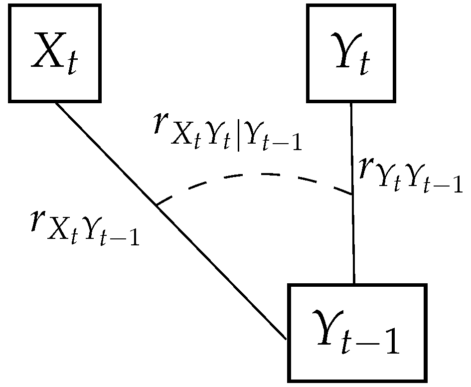
In this section, the univariate model briefly described in Section 2.1 is extended to account for dependence between two variables. Let us consider two dependent processes and that present additionally serial correlation. Similarly, as in the univariate case, . A good alternative to model these kinds of processes are vine copulas or simply vines. Vines were originally introduced in Joe [44], Cooke [36], and Bedford and Cooke [48] (see [49]). Vines are a graphical way of representing multivariate joint distributions. They are a generalization of dependence trees. Roughly, a vine on n elements is a nested set of trees where the edges of tree j are nodes on the tree for . In particular, regular vines are of interest. These are vines whose edges in tree j are connected as nodes in tree only if they share a common node in tree j. Vine copulas as dependence models assign a bivariate copula to each edge in the first tree of the vine and conditional bivariate copulas to the edges of every tree . For a formal definition and their statistical treatment see for example [45]. A graphical representation of a regular vine on 3 nodes is presented in Figure 1. The edges in Figure 1 are assigned copulas that are parametrized by rank correlation coefficients and a conditional rank correlation of . Rank correlations are denoted by r followed by a subscript indicating the respective variables and time step. For example, denotes the rank correlation between process Y at times t and .
Notice that the essential correlations that the model needs to capture are the temporal dependencies and and the cross-correlation . If the process is generated independently with the univariate conditional copula model discussed in Section 2.1, then all that is left is to induce the correct dependence and . This can be achieved by modeling conditional on both and with a vine as the one presented in Figure 1. can be sampled according to Equation (4) where and are the marginal distributions underlying and ( and their inverses). Notice that the time index t is omitted since both processes are stationary. Moreover, h is the conditional copula (and its inverse) operator, as it was established earlier, and v is as before, an independent uniform random variable on [0,1].
The modeling procedure for the generation of a continuous bivariate stochastic process may be summarized as:
- i
- Fit the appropriate marginal distributions characterising the random variables (or use the empirical distribution).
- ii
- Select suitable copulas , , and .
- iii
- Generate the first variable () using the univariate copula model from the previous subsection.
- iv
- Generate the second variable () using Equation (4).
2.3. First-Order Intermittent-Continuous Bivariate Processes
In this section, the algorithm introduced in Section 2.2 is expanded to take into account intermittency. Results are based on the methodology presented in Torres-Alves et al. [41]. The basic idea is the coupling of the copula models with Markov chains. Specifically, the intermittent process is split into two sub-processes, (i) a discrete state-time Markov Chain accounting for the occurrence of a certain environmental condition, and (ii) copula models accounting for “amounts”. For example, in the case of daily precipitation, the Markov chain model would simulate days with or without rain while the copula models would account for the amount of rain (mm) per day. In an intermittent process, a Markov Chain model accounts for two states: one for zero amount (i.e., a dry day) and one for larger than zero amount (i.e., a wet day). The first-order discrete state-time Markov process is described by:
Similar to previous subsections, while for a countable set S. The probabilities that express the chance of transition between states are called transition probabilities. Continuing with our example, the two states of precipitation could be and , thus . The probabilities of interest are defined as follows:
For the above probabilities it holds that and . These probabilities comprise the so-called transition-probability matrix:
This matrix characterizes the Markov chain, providing all the information necessary to reproduce the process. In this way, the probability of each state is explicitly simulated. Another way to approach intermittency could be by adopting mixed type distributions that consider the dry state as an atom of probability. These have been adopted in literature [50,51] but they will not be discussed in this text; however, they are theoretically compatible with the proposed copula models.
The way that intermittency has been approached, by splitting the main process into two sub-processes of occurrence and amount dictates that the generation algorithm cannot be continuous. Specifically, the generation of the ”occurrence” process must precede the “amount” process. In other words, the Markov chain must precede the copula time series.
Consequently, to generate a synthetic time series, the first step is to generate realizations of the Markov chain. This will define the different state blocks (i.e., sequences of wet and dry periods of time) of the time series. For the dry (zero amount state) block of the intermittent process, no further action is needed. What follows is the generation of the amount process for the wet blocks. This can be performed for each block by employing the univariate model of Equation (3). Then the continuous process can be generated conditionally on the intermittent one of the same time step using the vine copula model of Equation (4); however, dry blocks require special treatment. Naturally, zero amount does not allow the expression of dependence via a copula. To overcome this, the cross-correlation is treated implicitly by conditionalizing the continuous process distribution according to the two states, wet and dry.
On a final note, to preserve correctly the first-order auto-dependence structure of the continuous process the generation of blocks must be sequential. This means that the first realization of each block should be conditional on the final realization of the previous block. The generation procedure is schematized in Figure 2. Superscripts W and D denote the conditional wet and dry continuous process marginal distributions, respectively.
The generation algorithm is summarized below:
- i
- Fit the appropriate marginal distributions characterizing the RV’s.
- ii
- Select and fit the suitable copulas , , and .
- iii
- Calculate the transition-probability matrix of the Markov chain for the intermittent process . Simulate a desired length of the Markov sequence.
- iv
- Split the time series into dry and wet blocks.
- v
- Generate “blocks” representing using the univariate copula model (Equation (3)).
- vi
- Generate the wet block using the vine model of Equation (4) and the appropriate marginal distribution. Use as seed for the first value of the wet block the last value of the previous dry block.
- vii
- Generate the dry block using the vine model (Equation (3)) and the appropriate marginal distribution. Use as seed for the first value of the dry block the last value of the previous wet block.
2.4. Multivariate Processes
Equations (3) and (4) define univariate and bivariate models, respectively; however, using the vine decomposition, higher-order models can be can be defined. As it was discussed during the introduction, while such models that account for temporal and spatial dependence exist, they require the calculation of a great number of parameters and are limited in the dependence structures they can represent. The methodology described herein aims to approximate dependent processes in time and space (for example precipitation and evaporation from an arbitrary number of stations) while remaining parsimonious and flexible. The key of this methodology is to approximate the conditional distribution of the spatial and temporal dependence through repetitive sampling instead of inferring it theoretically. It should be noted that the use of repetitive sampling in the context of hydrology has been used in [52,53] for the coupling of different temporal scales.
For simplicity, let us first assume a two-dimensional case. Let us define a two-dimensional process where the superscripts denote, for example, a corresponding station and the subscripts the time step. Moreover, let us assume that the temporal and spatial dependence can be described by the first-order model of Equation (3). The methodology can be described in four steps:
- i
- Generate one realization of from based on the temporal model.
- ii
- Generate n realizations of based on according to the spatial model. These are denoted with a tilde and the superscript as .
- iii
- Generate n realizations of based on according to the temporal model. These are denoted with a tilde and the superscript as . The spatial and temporal realizations are all plausible realizations of , which implies that a section between the two sets exists.
- iv
- Identify the common space. This is performed by identifying the realizations that minimize the root mean squared error (RMSE).
Notice that RMSE in step iv above is not used as a goodness of fit measure but rather as a selection criterion between the spatial and temporal components of the model. Another way to approach this could be a Monte Carlo procedure where a convergence criterion is targeted; however, in the context of time series generation this would result in non-practical computational demand. Other measures for selection may be very well possible; however, investigating them is out of the scope of this paper since we focus mainly on the general methodology for simulating spatially diverse data sources.
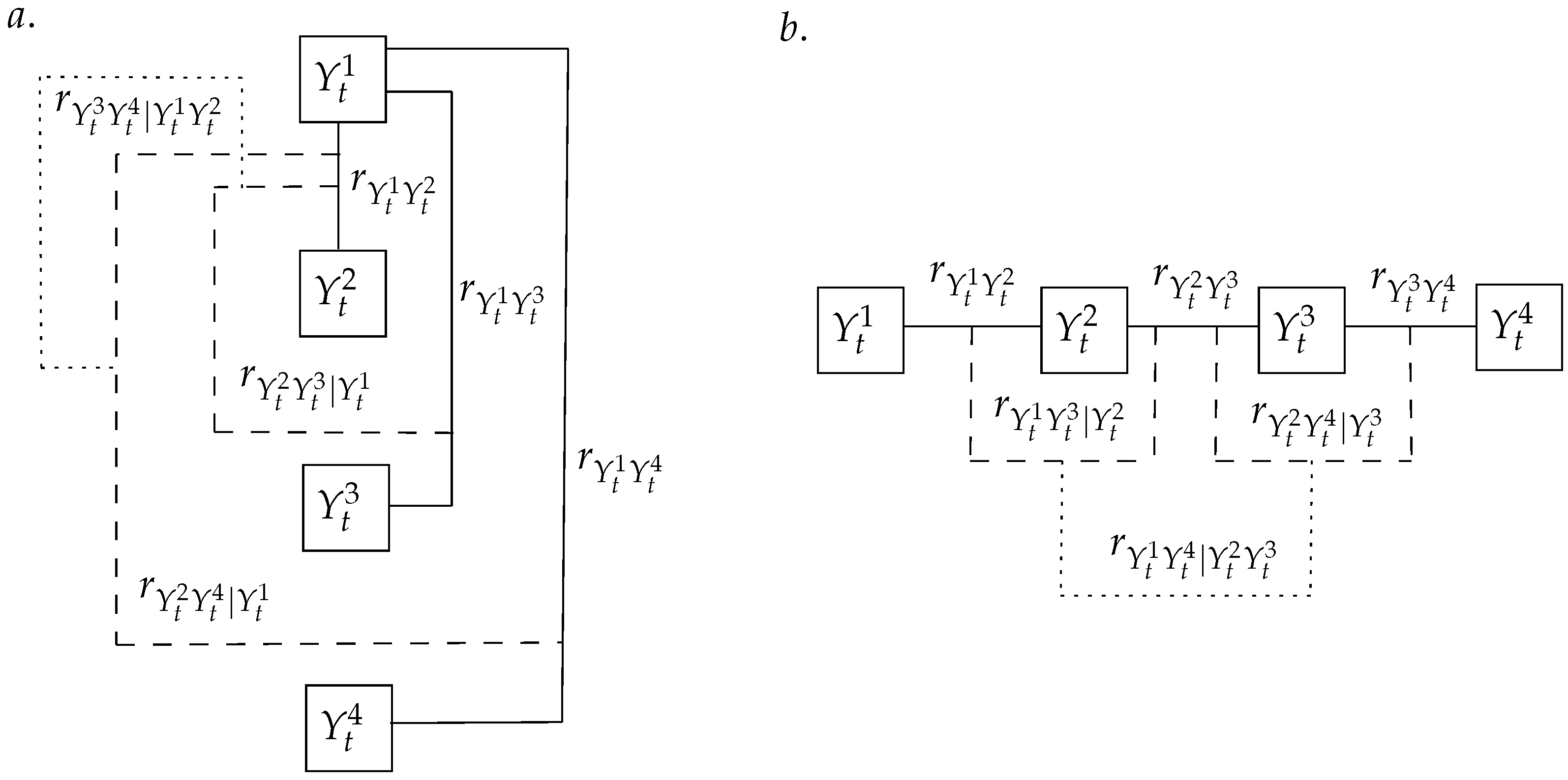
The above procedure can easily be extended to more dimensions. Let us consider another case where a set of four correlated variables is generated. It is reminded that the vine representation in four variables is not unique [54]. Two very common vines are the canonical or a C-Vine and the D-Vine. Their graphical representations are found in Figure 3.
It can be seen that the C-Vine representation has a unique variable, in our case , from which the other variables depend. On the contrary in the D-Vine representation, the variables depend serially. Both could be probable representations of spatial dependence; however, the algorithm depends on the vine’s sampling order. Let us assume that a C-Vine is selected. Further, let denote independent random draws from the uniform distribution. The sampling algorithm is given by the following equations:
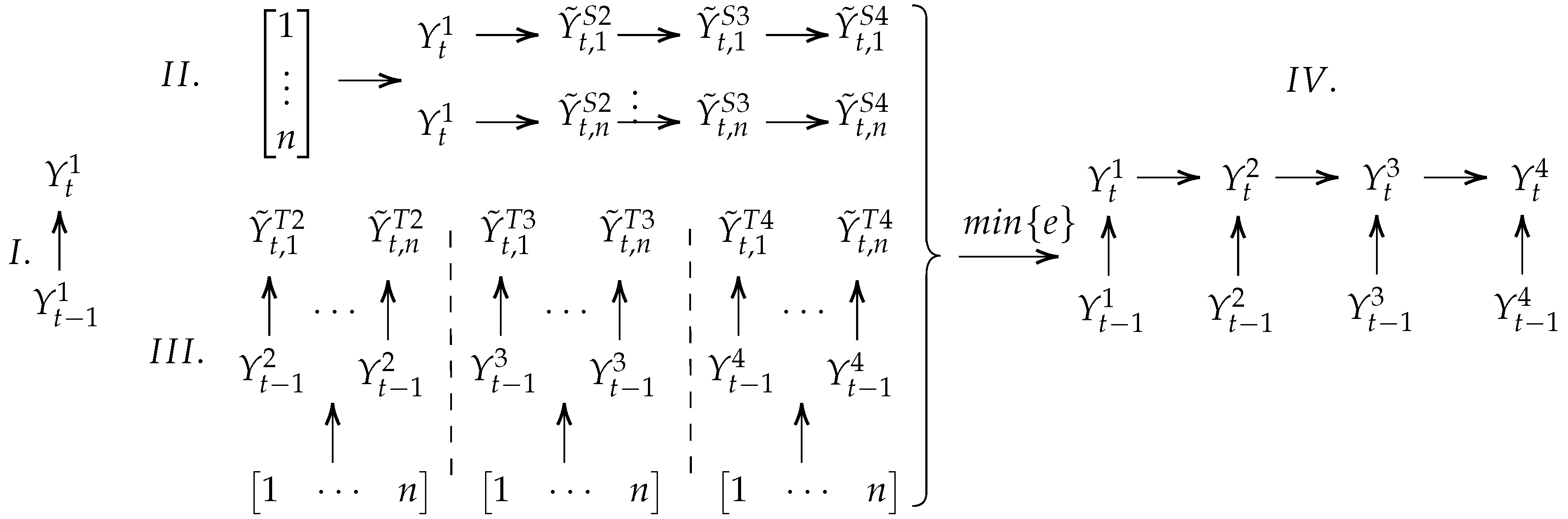
Furthermore, let us assume that the temporal dependence can be described by the first-order model of Equation (3). The first step is to generate a basis realization on which the repetitive sampling will be based. This decision depends on the selected spatial dependence model. It is noted that according to Equation (9), the C-Vine sampling order is 1-2-3-4. Thus, in this case, the algorithm should start by computing . If a D-Vine was selected instead, the algorithm should start by computing since the sampling order of a D-Vine is 3-2-4-1 [54]. The rest of the steps remain the same. n realizations are generated according to the spatial and temporal models of which the one that minimizes the RMSE (Equation (10)) is selected.
where in our case. This procedure is schematized in Figure 4.
The methodology above can be extended for m stations. The required number of parameters of such a model is:
The multivariate generation algorithm is summarized below:
- i
- Fit the appropriate marginal distributions characterizing the RV’s.
- ii
- Identify suitable models to describe spatial and temporal dependence.
- iii
- Select and fit suitable copulas to model dependencies.
- iv
- Select the number of trials n for the repetitive sampling.
- v
- Generate the first temporal realization according to the sampling order of the selected spatial model.
- vi
- Generate n realizations from the spatial and temporal models independently.
- vii
- Select the realization which minimizes the error (Equation (10)).
2.5. Admissible Marginal Distributions and Copula Fitting
One of the major benefits of modeling stochastic time series with copulas is the direct use of the marginal distribution, instead of moment approximations. This allows the utilization of classical fitting techniques such as maximum likelihood estimation [55] and L-Moments [56] and state-of-the-art methods such as K-Moments [14] and the metastatistical extreme value framework (MEV) [57]. Moreover, any finite variance distribution is admissible, which increases the flexibility of the models.
The same flexibility can be demonstrated in the admissible copula fitting techniques. In this study, the estimation of copula parameters is performed via the Spearman or Rank correlation coefficient accompanied by measures to test the goodness of fit, such as the Cramer–Von Mises statistic [58] and semi-correlations [43]; however, other methods such as maximum likelihood, Bayesian information criteria, or Kendall’s tau can be supported. A more comprehensive review can be found in [25,59].
3. Case Study
To demonstrate the effectiveness of the proposed vine copula model, two scenarios are presented: (i) simulation of daily evaporation and precipitation at one station and (ii) simulation of daily evaporation at four stations, all located at the Valley of Mexico. Additionally, the first scenario illustrates the influence of the dependence structure on the reliability of flood defenses.
The proposed methodology is validated on the accuracy of the reproduced historical characteristics, such as the approximation of the historical marginal distributions, the first-order auto-correlation dependence, and the cross-correlation dependence structure.
3.1. Area of Study
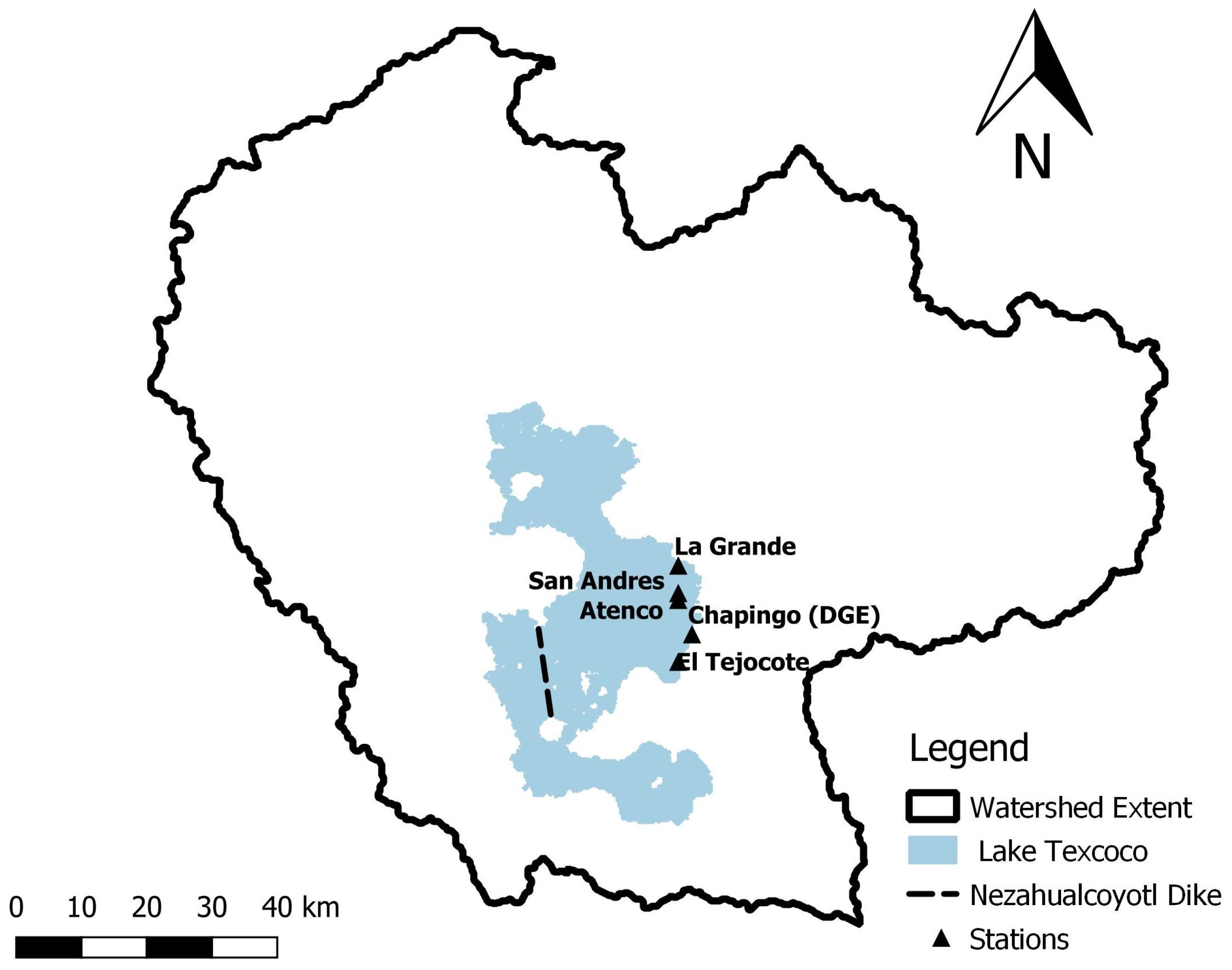
The case study described herein is presented in Torres-Alves & Morales-Nápoles (2020) [41]. It concerns the reliability analysis due to overflow of the ancient Nezahualcoyotl dike that was once located in the Valley of Mexico (Figure 5). The Aztecs built this structure around 1450 AD to protect their capital, the city of Tenochtitlan, from rising water levels in the lacustrine system.
Around 1519, the Valley of Mexico was covered by a lacustrine system comprising of six interconnected lakes. These lakes connected during high water and because of the salinity of the lakes, the rising water posed a threat to agriculture and freshwater supplies in Tenochtitlan. Nowadays, there are no remains of this dike and the lakes were almost completely drained by the end of the 19th century. Ref. [41] reconstructed the geometry and position of the ancient structure based on historical sources. The dike was 16 km long with a height of 8 m and a width of 3.5 m. It was made out of wood, stone, and mud. Moreover, ref. [41] estimated the extent of the lacustrine system and proposed a simple hydrological balance equation (Equation (12)) to compute the water level fluctuation at the lake. Finally, an assessment of the reliability of the dike due to overflow was presented.
where:
- is the precipitation at time t (m/day).
- is the evaporation at time t (m/day).
- is the tributary area of the basin (m).
- is the surface area of the lake (m).
- is the daily change in volume (m/day).
The hydrological balance was simulated only for the wet seasons. For this reason, an initial water level () needed to be assumed. The dike’s probability of failure due to overflow was computed for six initial water levels (1 to 6 m).
3.2. Data
To simulate the precipitation and evaporation time series, records from five stations situated within the Valley of Mexico are analyzed. This analysis was originally performed in [41]. Therefore, only a brief overview is provided in the present work. For a detailed presentation of the historical records the reader is referred to the original publication. The data are available from Mexico’s national database [60]. Information about the stations is given in Table 1.
In this region, two seasons are identified, (i) wet season (May–October), and (ii) dry season (November–April). The data from the stations were analyzed and appropriate distributions were fitted using Maximum likelihood (Table 2). The respective cumulative distribution functions are presented in Appendix A.
Furthermore, bivariate copulas were fitted for each data pair (precipitation–evaporation). The results are presented in Table 3. In [41] the authors use different goodness of fit (GOF) techniques to show that the pairs in Table 3 are adequate choices for the (conditional) copulas of interest. For further details about the GOF techniques used, the reader is referred to [41] and references therein. Their functional representations are given in Appendix B.
3.3. Simulation of Daily Evaporation and Precipitation
The simulation of precipitation and evaporation poses a particular challenge due to the intermittent behavior exhibited by precipitation. Moreover, these variables are the basic drivers for many hydrological models (i.e., [61]). Producing correlated time series enables the quantification of uncertainty in these drivers and a probabilistic description of the results. For this scenario, the data from Atenco station were analyzed (for further details on why this station is selected, refer to [41]). From these data, 5000 hypothetical wet seasons were generated, each with a length of 185 days.
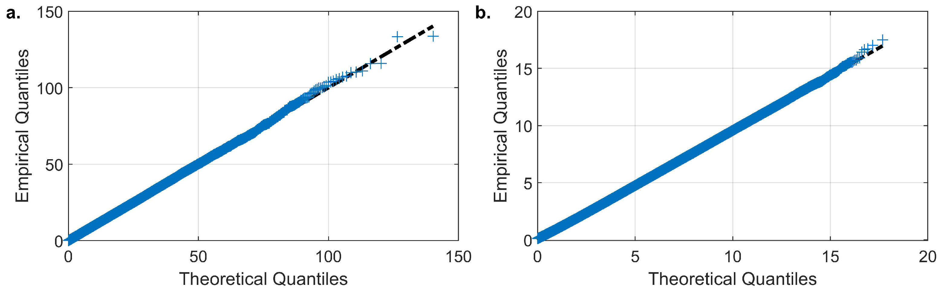
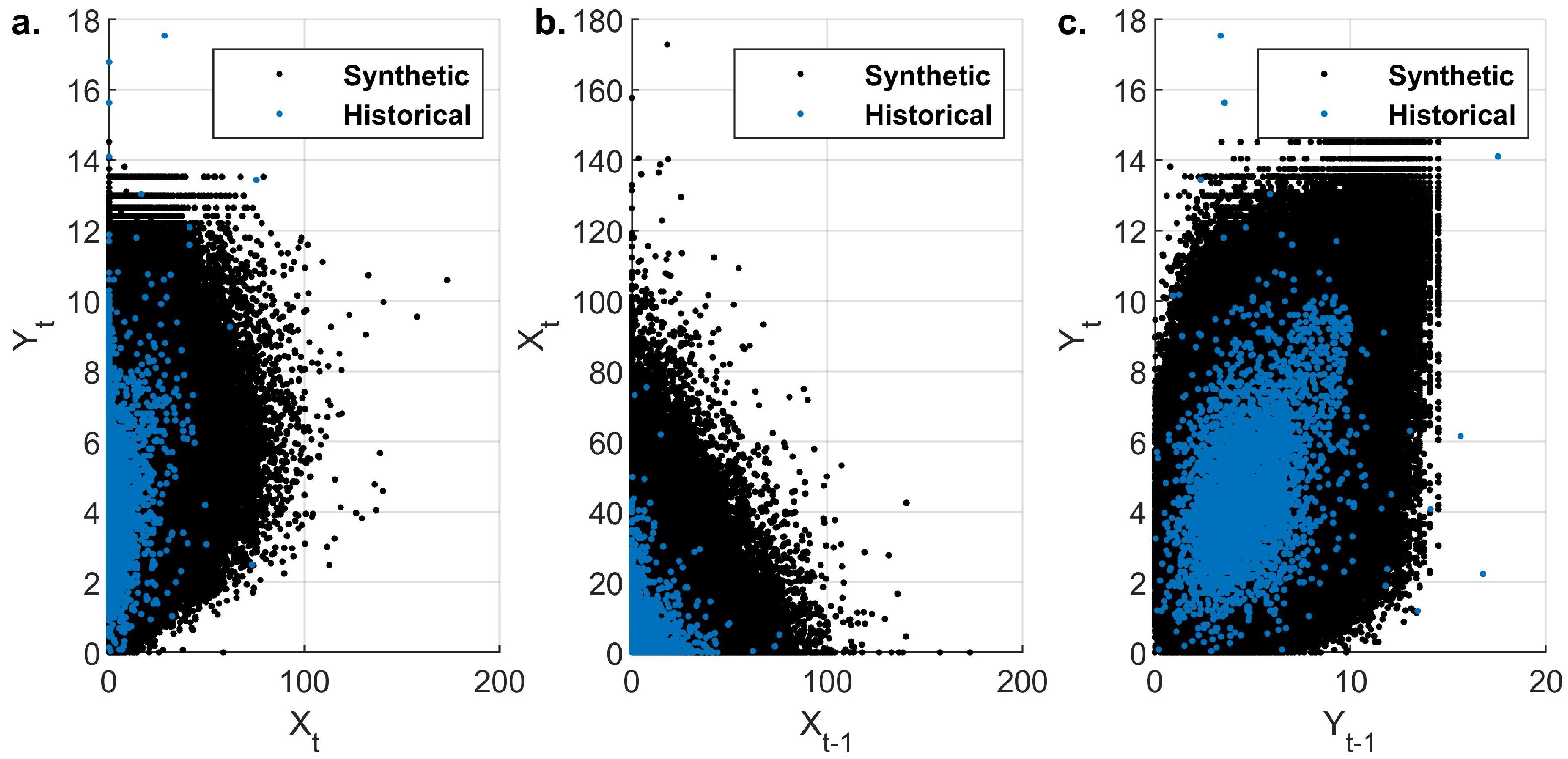
The ability of the model to reproduce the historical distributions is exhibited in Figure 6 with the use of QQ plots. These depict the relationship between the theoretical and empirical quantiles of the cumulative distribution function. In the presented case, the plotted quantiles form an almost straight line; thus, good agreement is found between historical and simulated CDFs for both variables. Figure 7 provides a comparison between historical and synthetic dependence structure in the real domain. Precipitation and evaporation exhibit a moderate correlation in the range of 0.3 to 0.4. Additionally, between the variables, a low negative correlation is observed. These dependencies are quantified in terms of rank correlations in Table 4. Overall, the model reproduces adequately the first-order auto-dependence as well as the dependence between variables.
The Effect of the Choice of Copula
For the description of the historical first-order auto-dependence, a Gumbel copula was employed; however, in non-copula models addressing directly the characteristics of the observed dependence structure is not straightforward. To demonstrate the importance of a correct dependence description, a reliability calculation will be performed using two sets of the synthetic time series. The first one will be the one generated during the previous section. The second one is a precipitation and evaporation pair with the auto-dependence of evaporation described by a Gaussian copula. The latter is selected for comparison purposes because it represents a simple dependence structure that is reproduced by commonly used linear Gaussian models and more recent models such as [50,51,53,62]. The results for both cases are summarized in Table 5.
Given an initial water level of = 1 m. the probability of failure computed for the Gaussian copula case is higher than the Gumbel case.
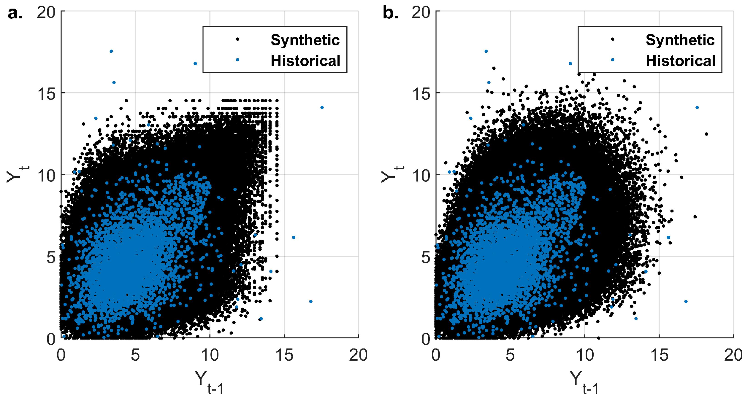
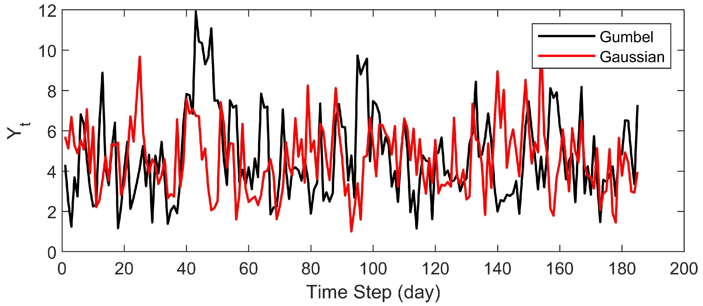
Note that the Gaussian copula reproduces the same first-order rank auto-correlation as the Gumbel. The difference can be entirely attributed to the change in the shape of the dependence structure (Figure 8). In the absence of tail dependence, there is no clustering of high evaporation events. This moderates the outgoing flux of the lake resulting in more frequent high-water levels and thus, a larger probability of failure. This can be illustrated by comparing the two evaporation time series (Figure 9).
In Figure 9, the time series generated by the Gumbel copula presents clusters of high evaporation values around time steps 40 to 70, 100 and 160. On the contrary, the time series generated by the Gaussian copula demonstrate a more symmetrical dependence pattern. This is in accordance with the scatter plots provided in Figure 8 where the difference of tail dependence between both copulas is demonstrated. Additionally, it is observed that the differences between the computed probabilities decrease as the initial water level increases (Table 5). This is because larger probabilities (smaller return periods) correspond to events further from the tail, where the differences between the copula functions are found. These results provide evidence on the importance of selecting an appropriate model that characterizes the dependence structure of extreme events.
3.4. Simulation of Evaporation across Multiple Stations
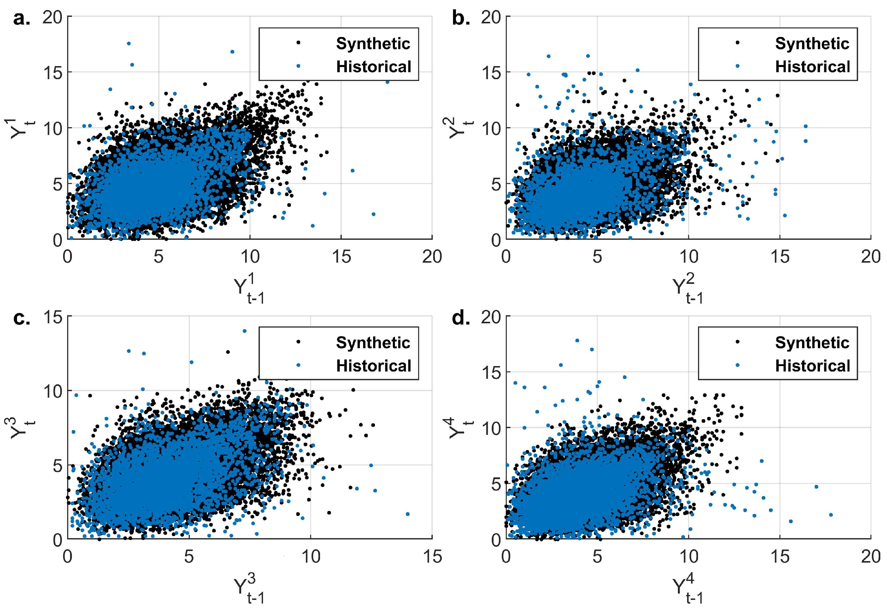
This section presents the application of the multivariate methodology. The developed multivariate algorithm is implemented for the simulation of daily evaporation in four of the five stations at the Valley of Mexico. Evaporation data from Atenco , La Grande , San Andres , and Chapingo (DGE) were used to generate 100 seasons (each of 185 days). The spatial dependence is described by a Gaussian copula while the temporal dependence is described by a Gumbel copula. For the latter, only the first-order auto-dependence is taken into account. The sampling number is set to . A comparison between historical and simulated first-order auto-dependence is provided in Figure 10.
On the temporal level, evaporation in all stations demonstrates a rank correlation in the range of 0.35 to 0.45. Moreover, the historical data exhibit upper tail dependence between consecutive time steps. In all cases, the simulated data reproduce the shape of the historical dependence structure. The results are quantified in Table 6 where a very good agreement is found between historical and simulated rank correlations.
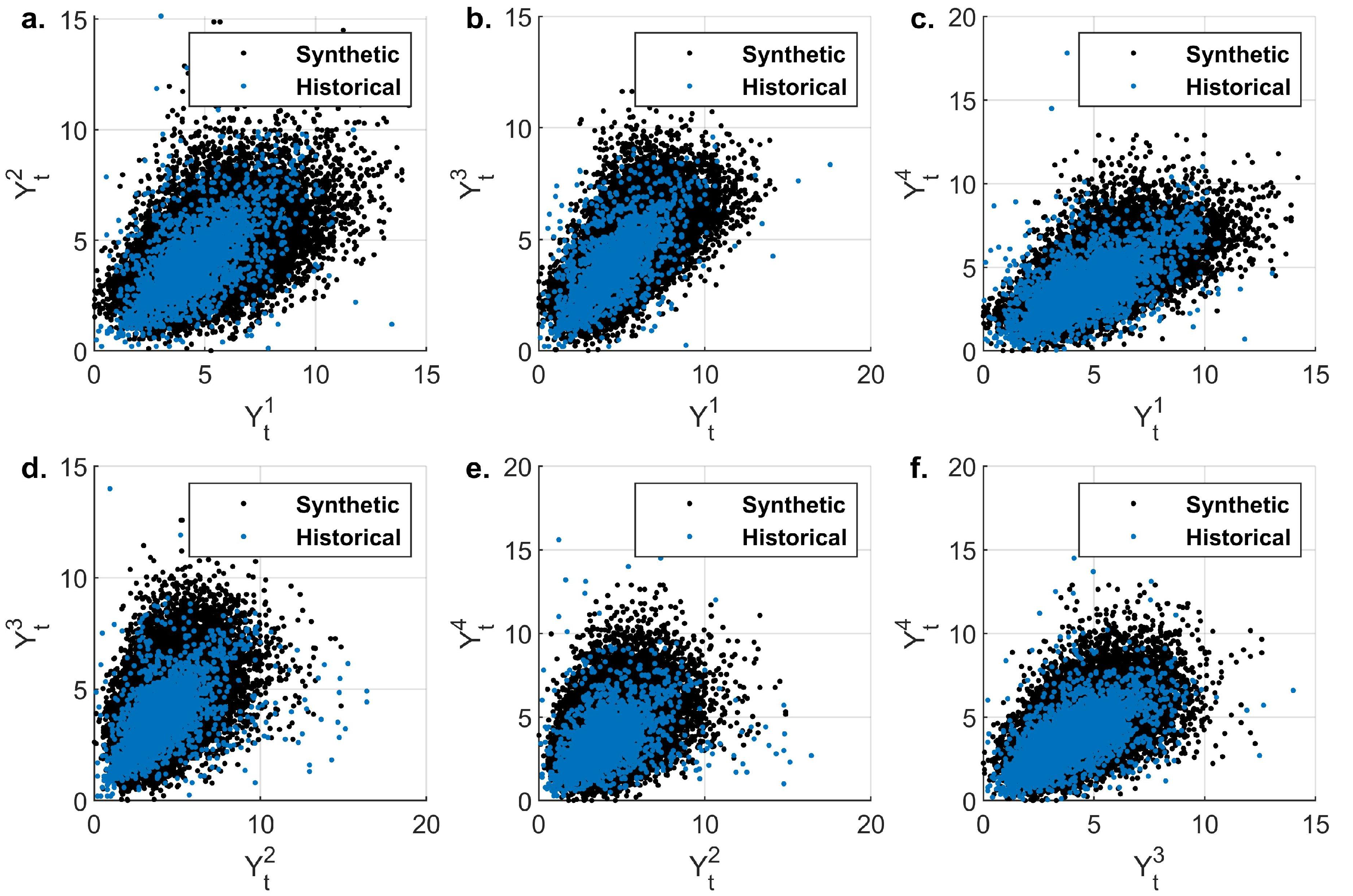
Furthermore, evaporation exhibits a high spatial correlation, in the order of among the stations. From a physical point of view, this can be explained by the proximity of the stations and their position within the same watershed. The proposed algorithm was able to reproduce these dependencies to a good extent (Figure 11); however, a small deviation is observed between pairs and (Table 7). This difference can be attributed to the copula choice.
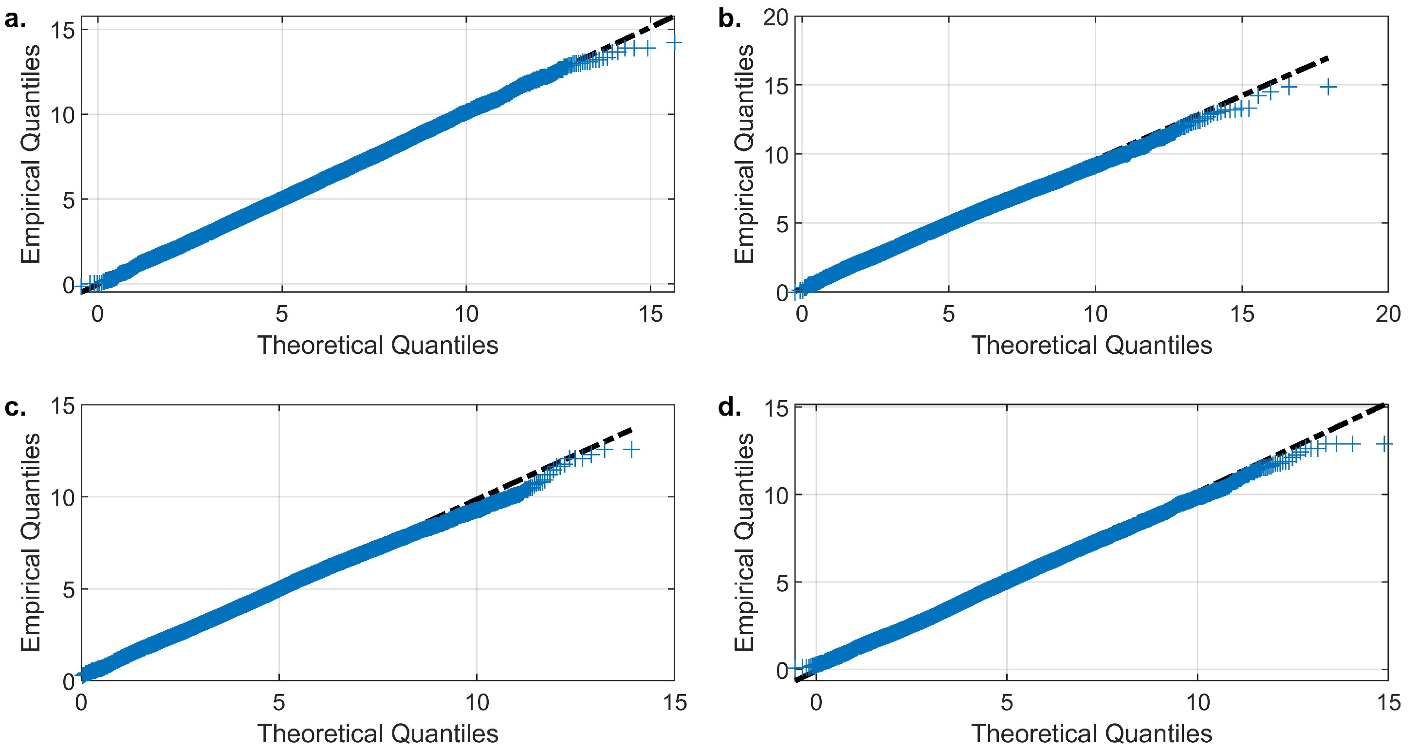
Finally, the model’s ability to reproduce the marginal distributions is presented in Figure 12 where the empirical and synthetic quantiles of the cumulative distribution function are compared. Overall, a good agreement is observed for all variables; however, small differences are found near the tails. The size of this disagreement is not atypical in hydrological research or other fields where uncertainty in modeling or observations is, in general, significant.
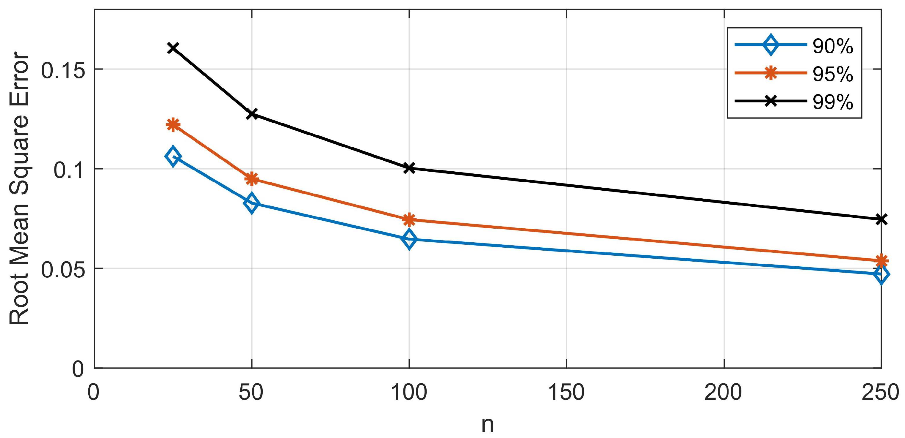
Exploration of the Repetitive Sampling Length
As with any repetitive sampling approach, the accuracy of the method depends upon the sampling length. To determine the relationship between accuracy and sampling length, four simulations were performed with and the empirical cumulative distributions of their RMSE (Appendix B) were computed. In Figure 13, the relationship between RMSE and sampling length for 90%, 95%, and 99% percentiles is plotted. As the sampling length increases, the RMSE decreases. The largest decrease can be found between and . For , the RMSE of the 99% percentile is equal to 0.1. The previous simulation suggests that this level of error yields adequate results. Furthermore, increasing the sampling length does not offer significant improvements in accuracy while at the same time it drastically increases the computational cost. From this perspective, a sampling length between 50 to 100 is a reasonable choice.
4. Conclusions
This paper presents a methodology to simulate hydroclimatic variables through copula-based models. The proposed methodologies focus on the use of vine copulas to characterize complex temporal and spatial probabilistic dependence. Two cases are presented: (i) the generation of correlated precipitation and evaporation on a daily scale and (ii) the generation of correlated daily evaporation time series from four stations. The first case consists of a trivariate vine copula to handle temporal dependence of evaporation and cross-dependence with precipitation. To capture intermittency, Markov chains were coupled with a copula-based model. In the second case, the methodology relied on repetitive sampling to couple the temporal and spatial vine copula models. The result is a parsimonious and flexible model capable of simulating accurately observations from an arbitrary number of stations.
In both case studies discussed herein, the models proved their capability to capture the underlying dependence structures, reproduce the marginal distributions, and intermittency. In fact, for the dependence structure, important asymmetries (such as tail dependence) may be incorporated. These asymmetries are often found but overlooked in the modeling of hydroclimatic variables. One of our case studies shows that by ignoring these asymmetries, the reliability of hydraulic structures, for example, could be underestimated by a factor of 2 in some cases (Table 5).
We have shown the ability of our approach combining Markov chains and vine copula models to reproduce short-range dependence (SRD) structures [63]. Many hydroclimatic processes however exhibit long-range dependence (LRD) [64,65,66]. The performance of our approach for these kind of dependence may be a subject for future research.
Author Contributions
Conceptualization, G.P., G.A.T.-A. and O.M.-N.; Formal analysis, G.P.; Methodology, G.P.; Supervision, G.A.T.-A. and O.M.-N.; writing—original draft preparation, G.P., writing—review and editing, G.P., G.A.T.-A. and O.M.-N. All authors have read and agreed to the published version of the manuscript.
Funding
This research was partially funded by the Eugenides Foundation.
Institutional Review Board Statement
Not applicable.
Informed Consent Statement
Not applicable.
Data Availability Statement
The precipitation and evaporation timeseries analysed herein are available from the Center for Scientific Research and Higher Education at Ensenada (Centro de Investigacion Cientifica y de Educacion Superior de Ensenada—CISECE) at http://clicom-mex.cicese.mx/ accessed on 10 September 2019.
Acknowledgments
The first author was partially funded by the Eugenides Foundation for this research, as part of his MSc studies scholarship.
Conflicts of Interest
The authors declare no conflict of interest. The funders had no role in the design of the study; in the collection, analyses, or interpretation of data; in the writing of the manuscript, or in the decision to publish the results.
Appendix A. Distribution Functions
Weibull
where is the shape parameter and is the scale parameter.
Generalized Extreme Value
where is the shape parameter, is the scale parameter and is the location parameter.
Appendix B. Inverse Conditional Copulas
Gaussian Copula
Gumbel Copula
where C is the copula function .
In the case of the Gumbel copula, the inverse of the h-function cannot be given analytically. The use of a numerical method is necessary, such as Secant, Newton–Raphson, or even brute force. It should be noted that convergence of the solution close to the tails can be difficult and can affect the reproduction of the marginal distribution and the desired dependence structure. Moreover, accuracy in the order of at least is required for reliable simulation results. This task can be computationally very expensive.
References
- Fiering, M.B. Streamflow Synthesis; Harvard University Press: Cambridge, MA, USA, 1967. [Google Scholar] [CrossRef]
- Klemeš, V.; Srikanthan, R.; McMahon, T.A. Long-memory flow models in reservoir analysis: What is their practical value? Water Resour. Res. 1981, 17, 737–751. [Google Scholar] [CrossRef]
- Vogel, R.M.; Stedinger, J.R. The value of stochastic streamflow models in overyear reservoir design applications. Water Resour. Res. 1988, 24, 1483–1490. [Google Scholar] [CrossRef]
- Tsoukalas, I.; Makropoulos, C. A Surrogate Based Optimization Approach for the Development of Uncertainty-Aware Reservoir Operational Rules: The Case of Nestos Hydrosystem. Water Resour. Manag. 2015, 29, 4719–4734. [Google Scholar] [CrossRef]
- Tsoukalas, I.; Makropoulos, C. Multiobjective optimisation on a budget: Exploring surrogate modelling for robust multi-reservoir rules generation under hydrological uncertainty. Environ. Model. Softw. 2015. [Google Scholar] [CrossRef]
- Papoulakos, K.; Pollakis, G.; Moustakis, Y.; Markopoulos, A.; Iliopoulou, T.; Dimitriadis, P.; Koutsoyiannis, D.; Efstratiadis, A. Simulation of water-energy fluxes through small-scale reservoir systems under limited data availability. Energy Procedia 2017, 125, 405–414. [Google Scholar] [CrossRef]
- Koutsoyiannis, D.; Economou, A. Evaluation of the parameterization-simulation-optimization approach for the control of reservoir systems. Water Resour. Res. 2003, 39. [Google Scholar] [CrossRef] [Green Version]
- Koskinas, A.; Tegos, A. StEMORS: A Stochastic Eco-Hydrological Model for Optimal Reservoir Sizing. Open Water J. 2020, 6, 1. [Google Scholar]
- Haberlandt, U.; Hundecha, Y.; Pahlow, M.; Schumann, A.H. Rainfall Generators for Application in Flood Studies. In Flood Risk Assessment and Management: How to Specify Hydrological Loads, Their Consequences and Uncertainties; Schumann, A.H., Ed.; Springer: Dordrecht, The Netherlands, 2011; pp. 117–147. [Google Scholar]
- Papalexiou, S.M.; Koutsoyiannis, D. A global survey on the seasonal variation of the marginal distribution of daily precipitation. Adv. Water Resour. 2016, 94, 131–145. [Google Scholar] [CrossRef]
- Kossieris, P. Exploring the Statistical and Distributional Properties of Residential Water Demand at Fine Time Scales. Water 2018, 10, 1481. [Google Scholar] [CrossRef] [Green Version]
- Thomas, H.A.; Fiering, M. Mathematical synthesis of streamflow sequences for the analysis of river basins by simulation. In Design of Water Resources-Systems; Harvard University Press: Cambridge, UK, 1962; pp. 459–493. [Google Scholar]
- Lombardo, F.; Volpi, E.; Koutsoyiannis, D.; Papalexiou, S.M. Just two moments! A cautionary note against use of high-order moments in multifractal models in hydrology. Hydrol. Earth Syst. Sci. 2014, 18, 243–255. [Google Scholar] [CrossRef] [Green Version]
- Koutsoyiannis, D. Knowable moments for high-order stochastic characterization and modelling of hydrological processes. Hydrol. Sci. J. 2019. [Google Scholar] [CrossRef] [Green Version]
- Koutsoyiannis, D.; Manetas, A. Simple Disaggregation by Accurate Adjusting Procedures. Water Resour. Res. 1996, 32, 2105–2117. [Google Scholar] [CrossRef]
- Tsoukalas, I.; Papalexiou, S.M.; Efstratiadis, A.; Makropoulos, C. A Cautionary Note on the Reproduction of Dependencies through Linear Stochastic Models with Non-Gaussian White Noise. Water 2018, 10, 771. [Google Scholar] [CrossRef] [Green Version]
- Beran, J. Statistics for Long-Memory Processes; Routledge: London, UK, 1994. [Google Scholar] [CrossRef]
- Lloyd, E.H.; Hurst, H.E.; Black, R.P.; Simaika, Y.M. Long-Term Storage: An Experimental Study. J. R. Stat. Society. Ser. A Gen. 1966, 129, 591. [Google Scholar] [CrossRef]
- Mandelbrot, B.B. Une classe de processus stochastiques homothétiques a soi: Application à la loi elimatoloeique de H. E. Hurst. C. R. Aead. Sci. 1965, 260, 3274–3277. [Google Scholar]
- Koutsoyiannis, D. The Hurst phenomenon and fractional Gaussian noise made easy. Hydrol. Sci. J. 2002, 47, 573–595. [Google Scholar] [CrossRef]
- Dimitriadis, P.; Koutsoyiannis, D.; Iliopoulou, T.; Papanicolaou, P. A Global-Scale Investigation of Stochastic Similarities in Marginal Distribution and Dependence Structure of Key Hydrological-Cycle Processes. Hydrology 2021, 8, 59. [Google Scholar] [CrossRef]
- Koutsoyiannis, D. A generalized mathematical framework for stochastic simulation and forecast of hydrologic time series. Water Resour. Res. 2000, 36, 1519–1533. [Google Scholar] [CrossRef] [Green Version]
- Efstratiadis, A.; Dialynas, Y.G.; Kozanis, S.; Koutsoyiannis, D. A multivariate stochastic model for the generation of synthetic time series at multiple time scales reproducing long-term persistence. Environ. Model. Softw. 2014, 62, 139–152. [Google Scholar] [CrossRef]
- Dupuis, D.J. Using Copulas in Hydrology: Benefits, Cautions, and Issues. J. Hydrol. Eng. 2007, 12, 381–393. [Google Scholar] [CrossRef]
- Genest, C.; Favre, A.C. Everything You Always Wanted to Know about Copula Modeling but Were Afraid to Ask. J. Hydrol. Eng. 2007, 12, 347–368. [Google Scholar] [CrossRef]
- Salvadori, G.; Michele, C.D. On the Use of Copulas in Hydrology: Theory and Practice. J. Hydrol. Eng. 2007, 12, 369–380. [Google Scholar] [CrossRef]
- Daneshkhah, A.; Remesan, R.; Chatrabgoun, O.; Holman, I.P. Probabilistic modeling of flood characterizations with parametric and minimum information pair-copula model. J. Hydrol. 2016, 540, 469–487. [Google Scholar] [CrossRef] [Green Version]
- Lu Chen, S.G. Copulas and Its Application in Hydrology and Water Resources, 1st ed.; Springer: Singapore, 2019; p. 290. [Google Scholar] [CrossRef]
- Zhang, L.; Singh, V.P. Copulas and Their Applications in Water Resources Engineering; Cambridge University Press: Cambridge, UK, 2019. [Google Scholar] [CrossRef] [Green Version]
- Lee, T.; Salas, J.D. Copula-based stochastic simulation of hydrological data applied to Nile River flows. Hydrol. Res. 2011, 42, 318–330. [Google Scholar] [CrossRef]
- Jeong, C.; Lee, T. Copula-based modeling and stochastic simulation of seasonal intermittent streamflows for arid regions. J. Hydro-Environ. Res. 2015, 9, 604–613. [Google Scholar] [CrossRef]
- Serinaldi, F. A multisite daily rainfall generator driven by bivariate copula-based mixed distributions. J. Geophys. Res. Atmos. 2009. [Google Scholar] [CrossRef] [Green Version]
- Leontaris, G.; Morales-Nápoles, O.; Wolfert, A. Probabilistic scheduling of offshore operations using copula based environmental time series—An application for cable installation management for offshore wind farms. Ocean Eng. 2016, 125, 328–341. [Google Scholar] [CrossRef] [Green Version]
- Bedford, T.; Daneshkhah, A.; Wilson, K.J. Approximate Uncertainty Modeling in Risk Analysis with Vine Copulas. Risk Anal. 2016, 36, 792–815. [Google Scholar] [CrossRef] [Green Version]
- Chatrabgoun, O.; Hosseinian-Far, A.; Chang, V.; Stocks, N.G.; Daneshkhah, A. Approximating non-Gaussian Bayesian networks using minimum information vine model with applications in financial modelling. J. Comput. Sci. 2018, 24, 266–276. [Google Scholar] [CrossRef] [Green Version]
- Cooke, R.M. Markov and entropy properties of tree and vines-dependent variables. In Proceedings of the ASA Section of Bayesian Statistical Science, Istanbul, Turkey, 16–18 August 1997. [Google Scholar]
- Pereira, G.; Veiga, A. PAR(p)-vine copula based model for stochastic streamflow scenario generation. Stoch. Environ. Res. Risk Assess. 2018, 32, 833–842. [Google Scholar] [CrossRef]
- Jäger, W.S.; Nápoles, O.M. A Vine-Copula Model for Time Series of Significant Wave Heights and Mean Zero-Crossing Periods in the North Sea. ASCE-ASME J. Risk Uncertain. Eng. Syst. Part Civ. Eng. 2017. [Google Scholar] [CrossRef] [Green Version]
- Sarmiento, C.; Valencia, C.; Akhavan-Tabatabaei, R. Copula autoregressive methodology for the simulation of wind speed and direction time series. J. Wind. Eng. Ind. Aerodyn. 2018. [Google Scholar] [CrossRef]
- Brechmann, E.C.; Czado, C. COPAR—multivariate time series modeling using the copula autoregressive model. Appl. Stoch. Model. Bus. Ind. 2015, 31, 495–514. [Google Scholar] [CrossRef] [Green Version]
- Torres-Alves, G.A.; Morales-Nápoles, O. Reliability Analysis of Flood Defenses: The Case of the Nezahualcoyotl Dike in the Aztec City of Tenochtitlan. Reliab. Eng. Syst. Saf. 2020, 107057. [Google Scholar] [CrossRef]
- Sklar, A. Fonctions de répartition à n dimensions et leurs marges. Publ. L’InstitutDe Stat. L’Université Paris 1959, 8, 229–231. [Google Scholar]
- Joe, H. Dependence Modeling with Copulas; Chapman & Hall/CRC Monographs on Statistics & Applied Probability; Taylor and Francis: Hoboken, NJ, USA, 2014. [Google Scholar]
- Joe, H. Families of m-variate distributions with given margins and m(m − 1)/2bivariate dependence parameters. In Distributions with Fixed Marginals and Related Topics; Rüschendorf, L., Schweizer, B., Taylor, M.D., Eds.; Lecture Notes–Monograph Series; Institute of Mathematical Statistics: Hayward, CA, USA, 1996; Volume 28, pp. 120–141. [Google Scholar] [CrossRef]
- Aas, K.; Czado, C.; Frigessi, A.; Bakken, H. Pair-copula constructions of multiple dependence. Insur. Math. Econ. 2009. [Google Scholar] [CrossRef] [Green Version]
- Morales-Nápoles, O.; Steenbergen, R.D.J.M. Large-Scale Hybrid Bayesian Network for Traffic Load Modeling from Weigh-in-Motion System Data. J. Bridge Eng. 2015, 20, 04014059. [Google Scholar] [CrossRef]
- Morales-Nápoles, O.; Steenbergen, R.D. Analysis of axle and vehicle load properties through Bayesian Networks based on Weigh-in-Motion data. Reliab. Eng. Syst. Saf. 2014, 125, 153–164. [Google Scholar] [CrossRef]
- Bedford, T.; Cooke, R.M. Vines—A new graphical model for dependent random variables. Ann. Statist. 2002, 30, 1031–1068. [Google Scholar] [CrossRef]
- Cooke, R.M.; Joe, H.; Aas, K. Vines arise. In Dependence Modeling: Vine Copula Handbook; World Scientific: Singapure, 2010. [Google Scholar] [CrossRef]
- Papalexiou, S.M. Unified theory for stochastic modelling of hydroclimatic processes: Preserving marginal distributions, correlation structures, and intermittency. Adv. Water Resour. 2018, 115, 234–252. [Google Scholar] [CrossRef]
- Tsoukalas, I.; Makropoulos, C.; Koutsoyiannis, D. Simulation of Stochastic Processes Exhibiting Any-Range Dependence and Arbitrary Marginal Distributions. Water Resour. Res. 2018, 54, 9484–9513. [Google Scholar] [CrossRef]
- Koutsoyiannis, D. Coupling stochastic models of different timescales. Water Resour. Res. 2001, 37, 379–391. [Google Scholar] [CrossRef] [Green Version]
- Tsoukalas, I.; Efstratiadis, A.; Makropoulos, C. Building a puzzle to solve a riddle: A multi-scale disaggregation approach for multivariate stochastic processes with any marginal distribution and correlation structure. J. Hydrol. 2019, 575, 354–380. [Google Scholar] [CrossRef]
- Kurowicka, D.; Cooke, R. Sampling algorithms for generating joint uniform distributions using the vine-copula method. Comput. Stat. Data Anal. 2007, 51, 2889–2906. [Google Scholar] [CrossRef]
- Coles, S. An Introduction to Statistical Modeling of Extreme Values; Springer: London, UK, 2001. [Google Scholar]
- Hosking, J.R.M. L-Moments: Analysis and Estimation of Distributions Using Linear Combinations of Order Statistics. (English). J. R. Stat. Soc. Ser. B Methodol. 1990, 52, 105–124. [Google Scholar] [CrossRef]
- Zorzetto, E.; Botter, G.; Marani, M. On the emergence of rainfall extremes from ordinary events. Geophys. Res. Lett. 2016, 43, 8076–8082. [Google Scholar] [CrossRef] [Green Version]
- Genest, C.; Rémillard, B.; Beaudoin, D. Goodness-of-fit tests for copulas: A review and a power study. Insur. Math. Econ. 2009, 44, 199–213. [Google Scholar] [CrossRef]
- Choroś, B.; Ibragimov, R.; Permiakova, E. Copula Estimation. In Copula Theory and Its Applications; Jaworski, P., Durante, F., Härdle, W.K., Rychlik, T., Eds.; Springer: Berlin/Heidelberg, Germany, 2010; pp. 77–91. [Google Scholar]
- CLICOM. CISECE-Centro de Investigacion Cientifica y deEducacion Superior de Ensenada. Available online: http://clicom-mex.cicese.mx/ (accessed on 10 September 2019).
- Savenije, H.H.G. HESS Opinions “Topography driven conceptual modelling (FLEX-Topo)”. Hydrol. Earth Syst. Sci. 2010, 14, 2681–2692. [Google Scholar] [CrossRef] [Green Version]
- Tsoukalas, I.; Efstratiadis, A.; Makropoulos, C. Stochastic Periodic Autoregressive to Anything (SPARTA): Modeling and Simulation of Cyclostationary Processes With Arbitrary Marginal Distributions. Water Resour. Res. 2018, 54, 161–185. [Google Scholar] [CrossRef]
- Ibragimov, R.; Lentzas, G. Copulas and long memory. Probab. Surv. 2017, 14, 289–327. [Google Scholar] [CrossRef]
- Koutsoyiannis, D. HESS Opinions “A random walk on water”. Hydrol. Earth Syst. Sci. 2010, 14, 585–601. [Google Scholar] [CrossRef] [Green Version]
- Koutsoyiannis, D. Climate change, the Hurst phenomenon, and hydrological statistics. Hydrol. Sci. J. 2003, 48, 3–24. [Google Scholar] [CrossRef]
- Markonis, Y.; Moustakis, Y.; Nasika, C.; Sychova, P.; Dimitriadis, P.; Hanel, M.; Máca, P.; Papalexiou, S. Global estimation of long-term persistence in annual river runoff. Adv. Water Resour. 2018, 113, 1–12. [Google Scholar] [CrossRef]
Figure 1.
Vine representation of a joint distribution in 3 nodes.

Figure 2.
Proposed bivariate (intermittent process , continuous process ) generation algorithm explanatory diagram. Superscripts W and D denote the conditional wet and dry continuous process marginal distributions, respectively.
Figure 2.
Proposed bivariate (intermittent process , continuous process ) generation algorithm explanatory diagram. Superscripts W and D denote the conditional wet and dry continuous process marginal distributions, respectively.

Figure 3.
Graphical representation of four-dimensional C-vine (a) and D-vine (b). Figures reconstructed from [54], with permission from Elsevier.
Figure 3.
Graphical representation of four-dimensional C-vine (a) and D-vine (b). Figures reconstructed from [54], with permission from Elsevier.

Figure 4.
Four-dimensional generation algorithm. The roman numerals denote the steps of the algorithm. Superscripts S and T denote a realization according to spatial and temporal models, respectively. The tilde denotes a possible realization.
Figure 4.
Four-dimensional generation algorithm. The roman numerals denote the steps of the algorithm. Superscripts S and T denote a realization according to spatial and temporal models, respectively. The tilde denotes a possible realization.

Figure 5.
Outline of the study area. Reconstructed from information taken from [41].
Figure 5.
Outline of the study area. Reconstructed from information taken from [41].

Figure 6.
Comparison between empirical and theoretical quantiles for Precipitation (a) and Evaporation (b).
Figure 6.
Comparison between empirical and theoretical quantiles for Precipitation (a) and Evaporation (b).

Figure 7.
Scatter plot presenting the dependence structure of historical and synthetic data. (a) Precipitation–Evaporation , (b) Precipitation–Precipitation , (c) Evaporation–Evaporation .
Figure 7.
Scatter plot presenting the dependence structure of historical and synthetic data. (a) Precipitation–Evaporation , (b) Precipitation–Precipitation , (c) Evaporation–Evaporation .

Figure 8.
Scatter plot comparison of generated Evaporation auto-dependence structures with (a) Gumbel copula and (b) Gaussian copula. Historical data plotted as reference.
Figure 8.
Scatter plot comparison of generated Evaporation auto-dependence structures with (a) Gumbel copula and (b) Gaussian copula. Historical data plotted as reference.

Figure 9.
Evaporation time series generated by Gumbel and Gaussian copulas.

Figure 10.
Scatter plot of historical and synthetic auto-dependence structures. (a) Atenco , (b) La Grande , (c) San Andres , and (d) Chapingo (DGE) stations.
Figure 10.
Scatter plot of historical and synthetic auto-dependence structures. (a) Atenco , (b) La Grande , (c) San Andres , and (d) Chapingo (DGE) stations.

Figure 11.
Scatter plot of historical and synthetic cross-dependence structure. (a) Atenco–La Grande , (b) Atenco–San Andres , (c) Atenco–Chapingo (DGE) (d) La Grande–San Andres , (e) La Grande–Chapingo (DGE) , and (f) San Andres–Chapingo (DGE) .
Figure 11.
Scatter plot of historical and synthetic cross-dependence structure. (a) Atenco–La Grande , (b) Atenco–San Andres , (c) Atenco–Chapingo (DGE) (d) La Grande–San Andres , (e) La Grande–Chapingo (DGE) , and (f) San Andres–Chapingo (DGE) .

Figure 12.
Empirical and theoretical quantiles comparison for (a) Atenco , (b) La Grande , (c) San Andres , and (d) Chapingo (DGE) stations.
Figure 12.
Empirical and theoretical quantiles comparison for (a) Atenco , (b) La Grande , (c) San Andres , and (d) Chapingo (DGE) stations.

Figure 13.
RMSE as a function of sampling length (n) for 90%, 95%, and 99% quantiles.


Table 1.
Summary of precipitation and evaporation information for each station.
| Code | Name | Coordinates | Time Period | |
|---|---|---|---|---|
| Longitude | Latitude | |||
| 15008 | Atenco | −98.92 | 19.54 | 1 January 1961–22 August 2013 |
| 15044 | La Grande | −98.92 | 19.58 | 1 January 1964–31 August 2014 |
| 15083 | San Andres | −98.92 | 19.53 | 1 May 1967–31 December 2014 |
| 15167 | El Tejocote | −98.92 | 19.44 | 1 December 1957–1 January 2007 |
| 15170 | Chapingo (DGE) | −98.9 | 19.48 | 13 March 1957–1 January 2000 |
Table 2.
Selected distributions for all variables and stations.
| Station | Probability Distribution Function | |
|---|---|---|
| Precipitation | Evaporation | |
| Atenco | Weibull | Generalized Extreme Value |
| La Grande | Weibull | Generalized Extreme Value |
| San Andres | Weibull | Generalized Extreme Value |
| El Tejocote | Weibull | Generalized Extreme Value |
| Chapingo (DGE) | Weibull | Generalized Extreme Value |
Table 3.
Selected copula pairs for all stations.
| Pairs | Atenco | La Grande | San Andres | El Tejocote | Chapingo (DGE) |
|---|---|---|---|---|---|
| Gauss | Gauss | Gauss | Gauss | Gauss | |
| Gumbel | Gumbel | Gumbel | Gumbel | Gumbel | |
| Gumbel | Gumbel | Gumbel | Gumbel | Gumbel |
Table 4.
Comparison of historical and simulated rank correlations.
| Historical | 0.27 | 0.4 | −0.22 |
| Synthetic | 0.27 | 0.37 | −0.18 |
Table 5.
Probability of failure for different initial water levels () as calculated with the Gaussian and Gumbel time series.
Table 5.
Probability of failure for different initial water levels () as calculated with the Gaussian and Gumbel time series.
| Water Level at the Foot of the Dike (m) () | m.a.s.l. | Gaussian Copula | Gumbel Copula | ||
|---|---|---|---|---|---|
| Return Period (Years) | Return Period (Years) | ||||
| 1 | 2231 | 0.00171 | 586 | 0.00099 | 1006 |
| 2 | 2232 | 0.02641 | 38 | 0.02068 | 48 |
| 3 | 2233 | 0.16189 | 6 | 0.14956 | 7 |
| 4 | 2234 | 0.45131 | 2 | 0.44657 | 2 |
| 5 | 2235 | 0.74568 | 1 | 0.75102 | 1 |
| 6 | 2236 | 0.91468 | 1 | 0.92038 | 1 |
Table 6.
Comparison of historical and simulated rank auto-correlations.
| Historical | 0.41 | 0.36 | 0.45 | 0.44 |
| Synthetic | 0.41 | 0.37 | 0.46 | 0.40 |
Table 7.
Comparison of historical and simulated rank cross-correlations.
| Historical | 0.57 | 0.70 | 0.70 | 0.50 | 0.48 | 0.63 |
| Synthetic | 0.60 | 0.70 | 0.62 | 0.56 | 0.50 | 0.63 |
Publisher’s Note: MDPI stays neutral with regard to jurisdictional claims in published maps and institutional affiliations. |
© 2021 by the authors. Licensee MDPI, Basel, Switzerland. This article is an open access article distributed under the terms and conditions of the Creative Commons Attribution (CC BY) license (https://creativecommons.org/licenses/by/4.0/).
Share and Cite
MDPI and ACS Style
Pouliasis, G.; Torres-Alves, G.A.; Morales-Napoles, O. Stochastic Modeling of Hydroclimatic Processes Using Vine Copulas. Water 2021, 13, 2156. https://doi.org/10.3390/w13162156
AMA Style
Pouliasis G, Torres-Alves GA, Morales-Napoles O. Stochastic Modeling of Hydroclimatic Processes Using Vine Copulas. Water. 2021; 13(16):2156. https://doi.org/10.3390/w13162156
Chicago/Turabian StylePouliasis, George, Gina Alexandra Torres-Alves, and Oswaldo Morales-Napoles. 2021. "Stochastic Modeling of Hydroclimatic Processes Using Vine Copulas" Water 13, no. 16: 2156. https://doi.org/10.3390/w13162156
Note that from the first issue of 2016, this journal uses article numbers instead of page numbers. See further details here.