Numerical Modeling of Saltwater Intrusion in the Rmel-Oulad Ogbane Coastal Aquifer (Larache, Morocco) in the Climate Change and Sea-Level Rise Context (2040)

Abstract

Many coastal aquifers have experienced seawater intrusion (SWI) into fresh groundwater aquifers. The principal causes of SWI include over-pumping and events such as climate change (CC) and rising sea levels. In northern Morocco, the Rmel-Oulad Ogbane coastal aquifer (ROOCA) supplies high-quality groundwater for drinking water and agriculture. This favorable situation has led to increased pumping, resulting in environmental challenges such as dropping water table and SWI. Furthermore, the climate has resulted in less recharge, with an estimated annual precipitation of 602 mm and an average temperature of 18.5 °C. The goal of this study is to determine how CC, over-pumping, and sea-level rise (SLR) affect SWI. Computational groundwater and solute transport models are used to simulate the spatial and temporal evolution of hydraulic heads and groundwater solute concentrations. The calibration is based on steady and transient groundwater levels from 1962 to 2040. SWI simulations show that the NW sector of the coastal area would be polluted, with the toe reaching 5.2 km inland with a significant salinity (15–25 g/L). To protect the fresh water in the reservoir from SWI, enhanced groundwater development and management approaches for this aquifer are required, such as artificial recharge from surface water.

1. Introduction

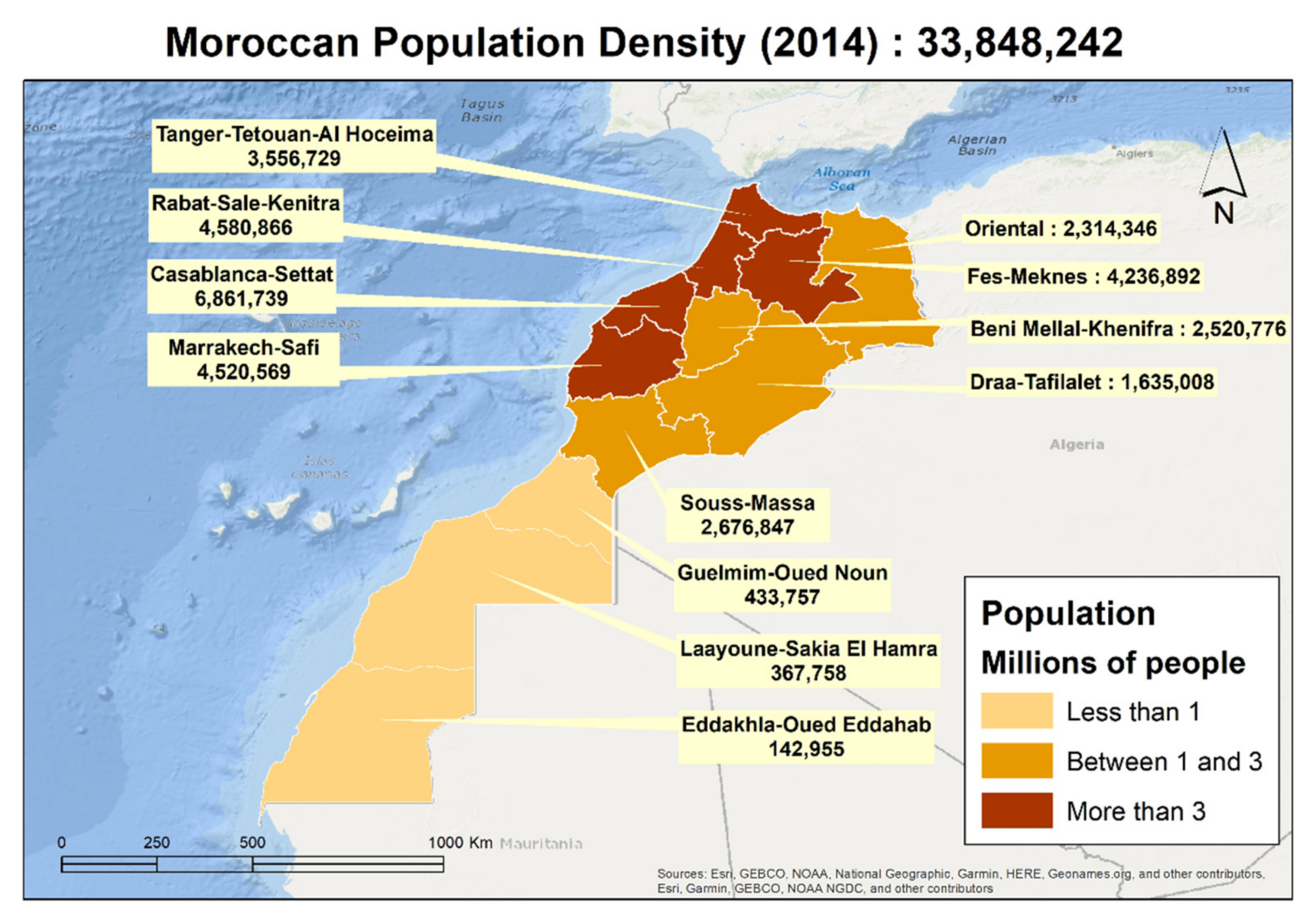
Seawater intrusion (SWI) is a worldwide problem that has been exacerbated by rising sea levels, climate change (CC), and excessive over-pumping (EOP) of coastal fresh groundwater (GW) resources. Many of the world’s coastal areas are characterized by dense settlements, with a large part of the world’s population residing within 60 km from the coast [1]. More than 3 million Moroccans live in Morocco’s coastal areas, and this figure is gradually increasing [2]. Indeed, in 2015, more than half of the population lived on the coast, which experienced drought and agricultural development with an increasing proportion of the rural population due to rural flight [2]. As a result, GW overexploitation soon became a widespread problem, with several coastal regions around the world (Morocco [3,4,5,6], Tunisia [7,8,9], Libya [10], Italy [11], and the Netherlands [1]) experiencing substantial SWI in aquifers, resulting in significant degradation of GW quality and, consequently, quantity [12,13,14,15,16].

To better understand the saltwater intrusion process, numerous studies have been undertaken, including laboratory-scale investigations and numerical and analytical modeling studies [17,18,19]. A probabilistic numerical model was built to predict the extent of saltwater intrusion into a coastal phreatic aquifer by Felisa et al. [17]. Fahs et al. [18] used the semianalytical solution of the dispersive Henry problem based on the Fourier technique to simulate heterogeneous and anisotropic coastal aquifers, taking into account the effects of the aquifer hydraulic parameters, boundary conditions, pumping and recharge rates, and aquifer depth. The effects of aquifer bed slope and seaside slope on saltwater intrusion were investigated by Abdelhamid et al. [19] to examine the movement of the dispersion zone under different settings of bed and seaside slopes, and a numerical model (SEAWAT) was applied to the well-known Henry problem.

Nowadays, numerical modeling technology is an important tool for GW analysis. CC impacts, computational GW flow, and transport modeling have been investigated in many regions around the world [20,21,22,23,24,25,26,27,28,29].

The impact of CC and sea-level rise (SLR) on SWI has been studied using a variety of models. Abd-Elhamid et al. [30] examined the individual and combined effects of predicted SLR and over-pumping on SWI using a coupled transient density-dependent finite element model to simulate SWI in the Gaza aquifer. Ranjbar [31] analyzed the effects of a 1 m gradual and immediate SLR associated with pumping activities on the location of seawater wedge toe in a shallow coastal aquifer on the Caspian Sea’s southern shores. Essink and Schaars [32] developed a model to simulate GW flow, heat and salinity distribution, and seepage and salt load flux into the surface water system. The model was used to analyze the impact of future events such as CC, SLR, and land submergence, as well as human activities, on the GW system’s qualitative and quantitative features. Tiruneh and Motz [33] used SEAWAT to explore the influence of SLR on the freshwater–saltwater interface, taking pumping and recharging into account. Canning [34] presented the climatic variability certainty and uncertainty for Washington’s maritime water. He also gave a history of SLR in Puget Sound as a result of CC. All of these studies have demonstrated the importance of numerical modeling methods in the monitoring and successful management of coastal aquifers. Furthermore, the use of numerical models in distinct case studies provides significant obstacles due to site-specific properties of individual aquifers. Moreover, these models are crucial for developing curative solutions to reduce SWI. In earlier research, various approaches have been recommended, including artificial recharge (Yang et al. [35]; Hussain et al. [36]); abstraction, desalination, and recharge (ADR) approach (Abd-Elhamid and Javadi [37]); reduced pumping rates (Sherif et al. [38]; Rejani et al. [39]); relocation of the pumping wells (Datta et al. [40]; Mantoglou and Papantoniou [41]); subsurface dams (Chang et al. [42]); and cutoff walls (Shen et al. [43]; Abdoulhalik and Ahmed [44]).

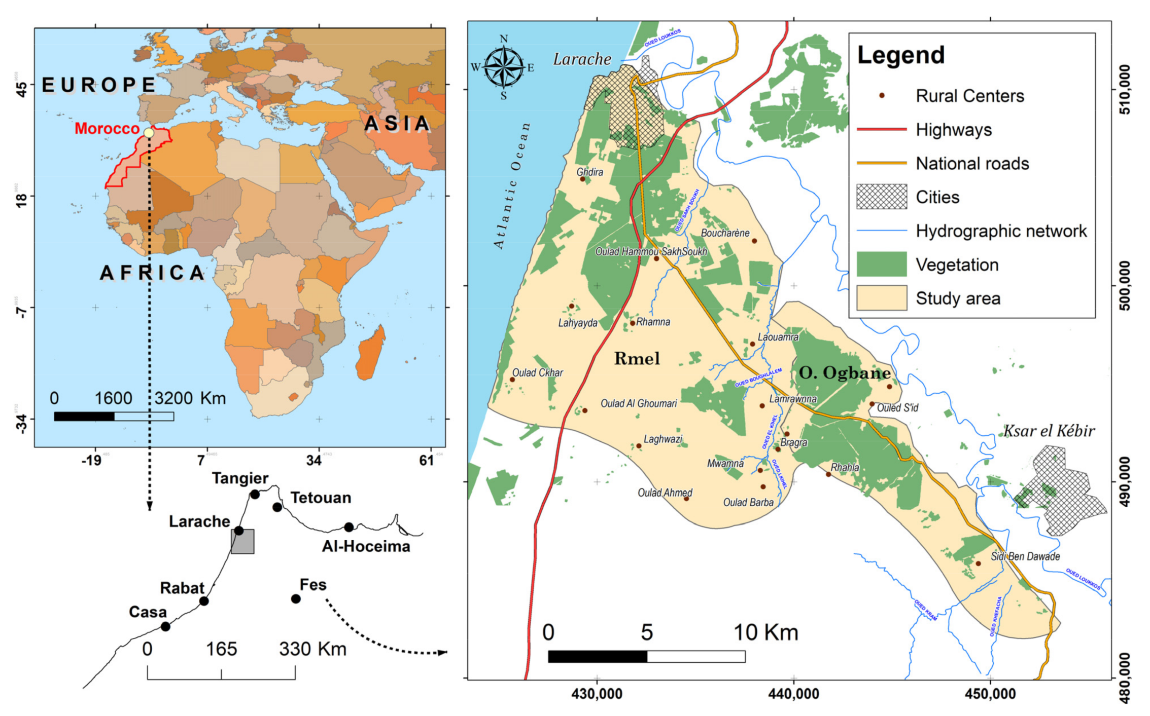
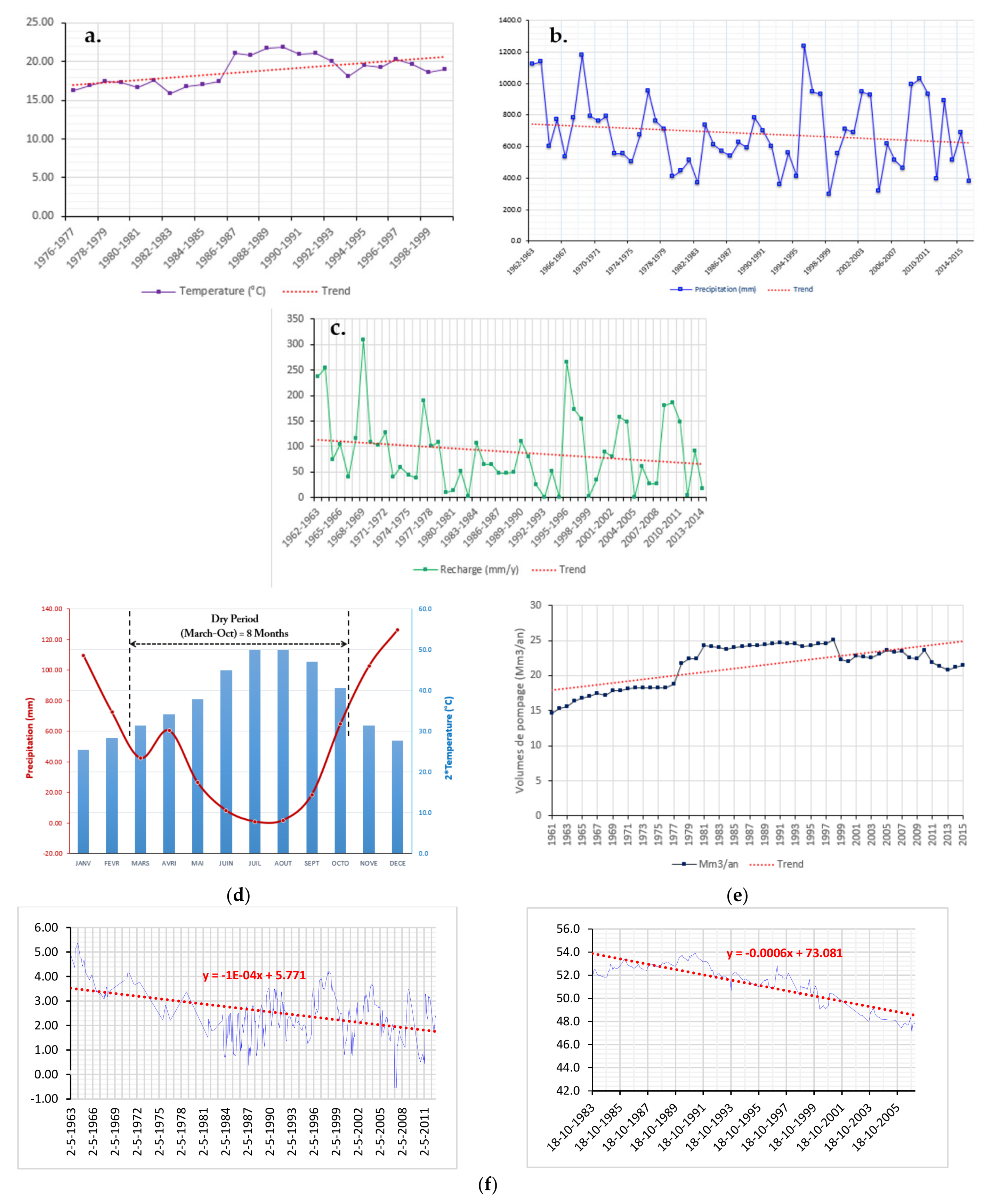
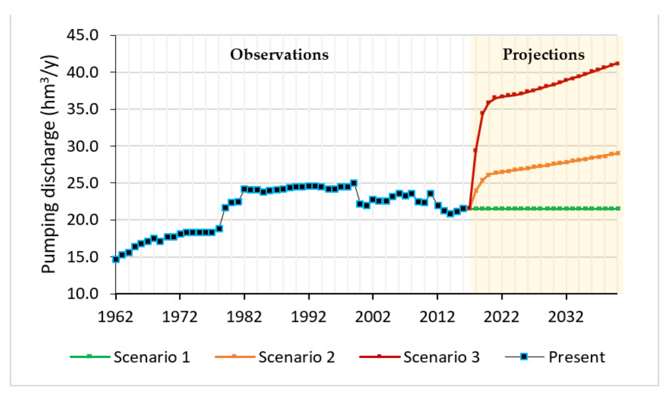
The Rmel-Oulad Ogbane coastal aquifer (ROOCA), situated in Morocco’s northwest, is well-known for its contribution to agricultural, economic, and social growth. Furthermore, GW is the sole source of domestic use for the urban and rural populations. The decrease in average rainfall from 1211 mm in 1963 to 378 mm in 2016 is attributable to the effects of CC, which triggers intermittent droughts and reductions in recharge, which directly influence the GW level; the effects of CC also include the influence of SLR on the GW level and salinity intrusion. This condition is aggravated by ROOCA EOP values ranging from 14.6 hm³ in 1961/62 to 21.52 hm³ in 2015/16, which are used in rural, urban, and agricultural areas for industrial and drinking water supply [45]. This has culminated in a significant decrease in GW levels, which could potentially result in an aquifer water balance deficit, in addition to a depletion in GW from the reservoir and a high standard SWI in the coastal plains, posing a severe challenge to potential water supplies. 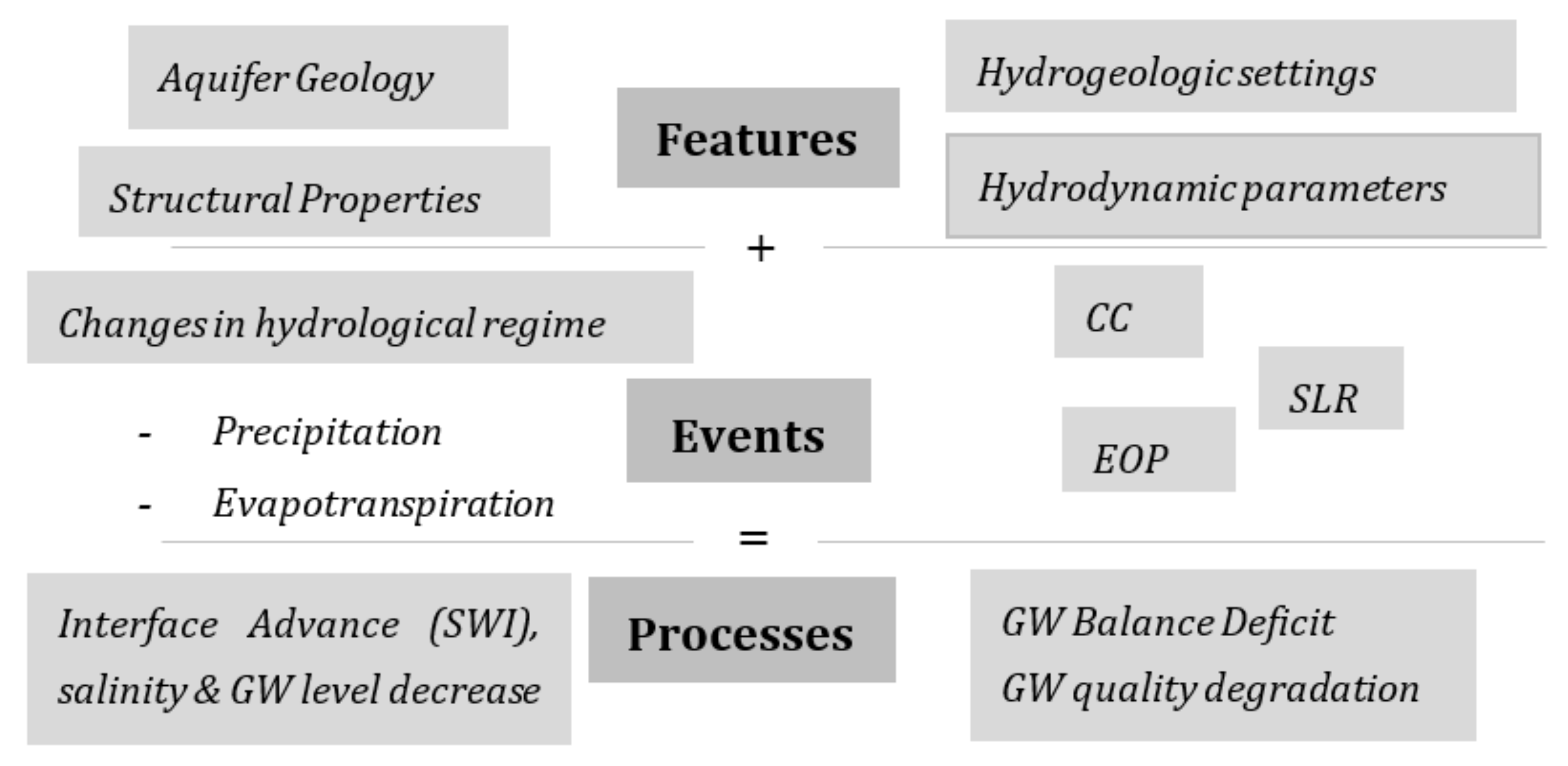Figure 1 summarizes mechanisms that affect coastal aquifers such as ROOCA. As a result, careful management of GW potential in these aquifer systems is needed, as is consideration of the CC. It is possible to create it using a methodological approach that combines geographic information system (GIS), climate parameters, and the numerical GW flow model, which is suggested and extended to the case of ROOCA in Morocco. This enables one to comprehend the factors that control the activity of the coastal aquifer’s freshwater/saltwater transition region under multiple input conditions and CC scenarios, such as Representative Concentration Pathway (RCP) 4.5 and RCP 8.5, which are two different types of pathways in CC. These instruments would help municipal water supply agencies in their economic and water resource growth planning.

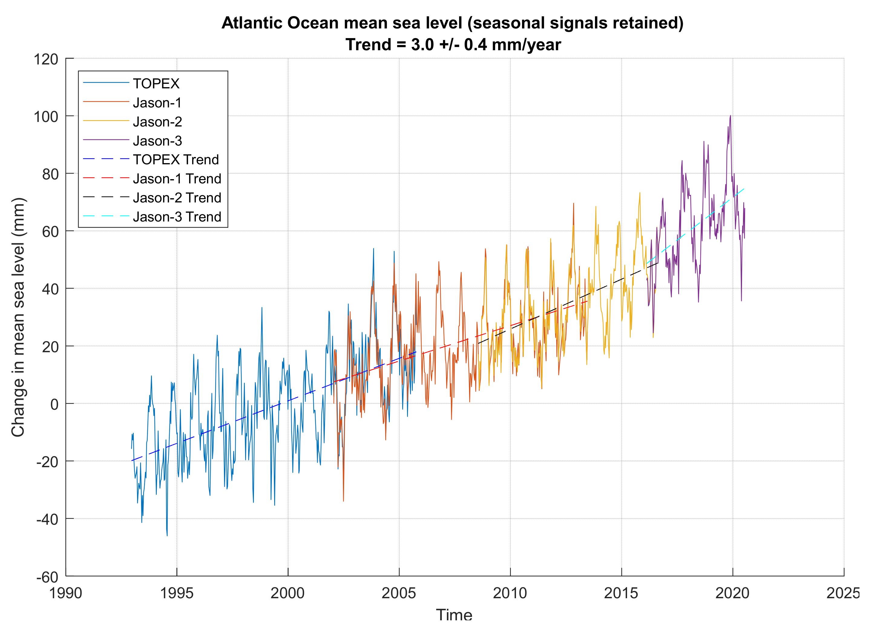
Ocean warming and ice melting, according to the Intergovernmental Panel on Climate Change (IPCC), could raise global sea levels by up to ~60 cm by 2100 [46].

The effects of climate-induced SLR will become more apparent as the intensity of the phenomenon increases, especially in low-elevation coastal areas (Figure 2). The majority of African countries tend to be in grave danger due to low levels of development along with projections of fast population increases in coastal areas. Under these conditions, the SLR at the aquifer’s seaside boundary, which is an additional pressure head, would be imposed. Water table gradient and/or the piezometric head would decrease, resulting in further interference. Many hydraulic, geometric, and transport parameters influence the SWI operation. Each aquifer has its set of circumstances, and the sharp interface approach cannot be applied to all of them, because of the transient conditions which often reign in the exploitation of aquifers.

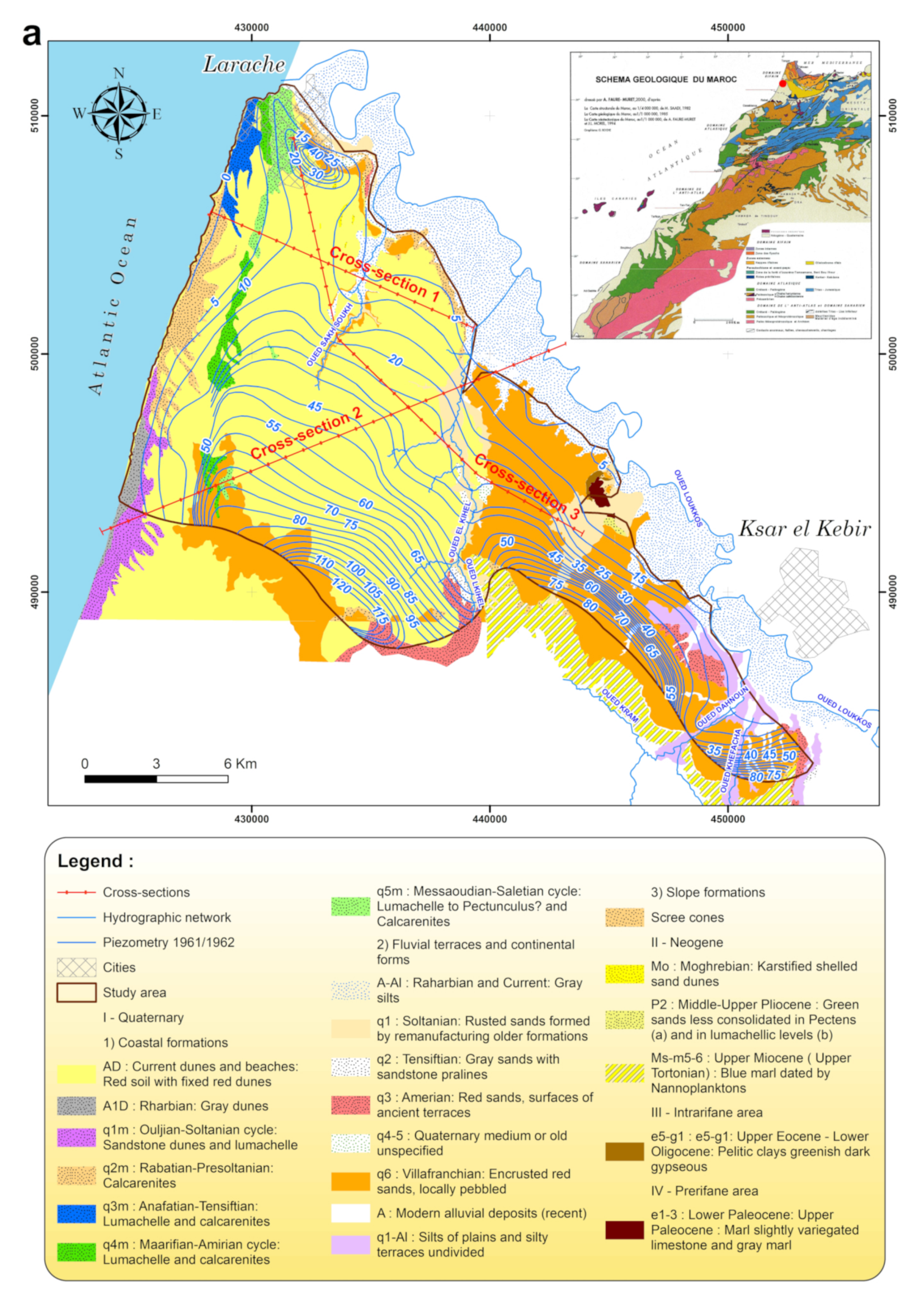
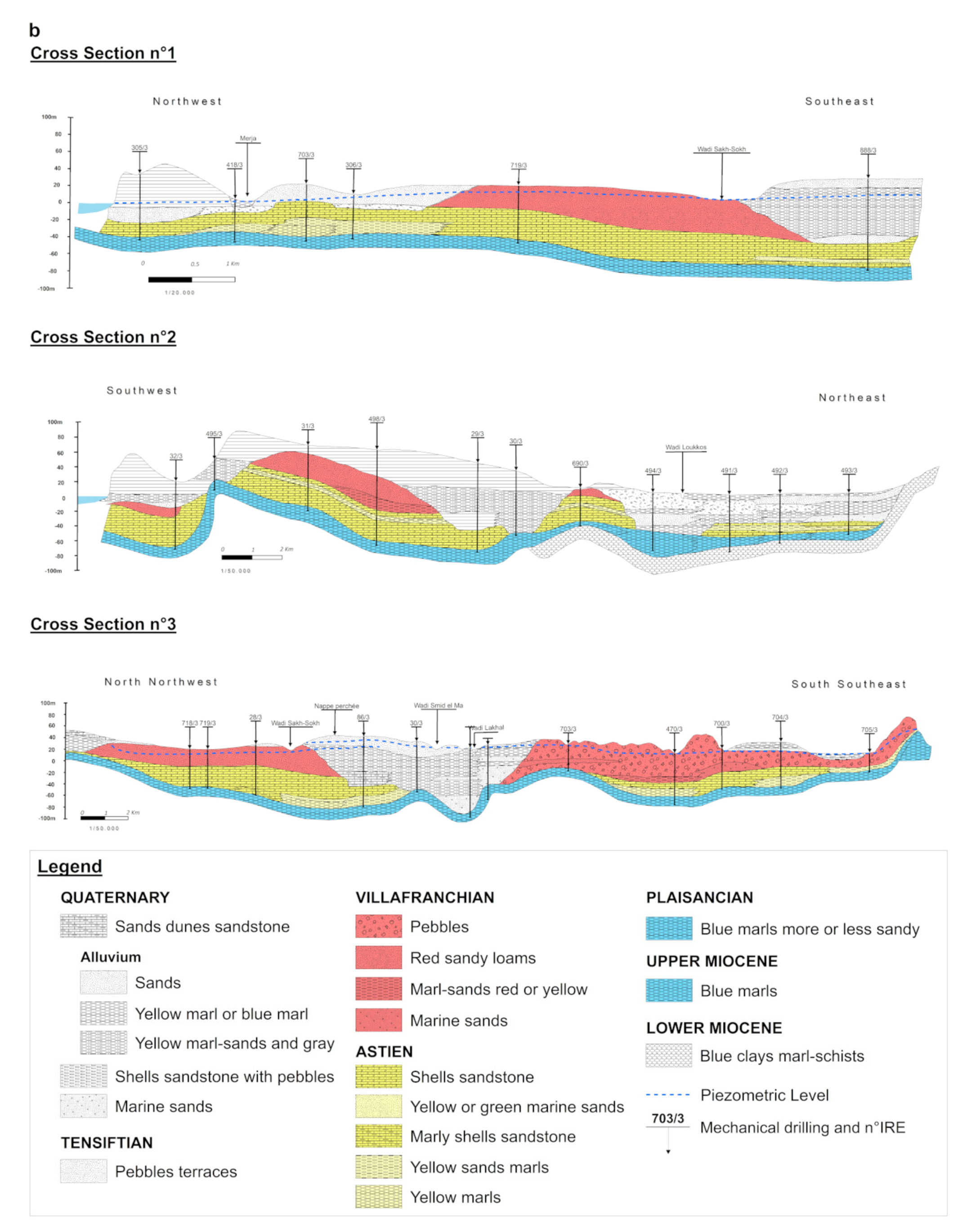
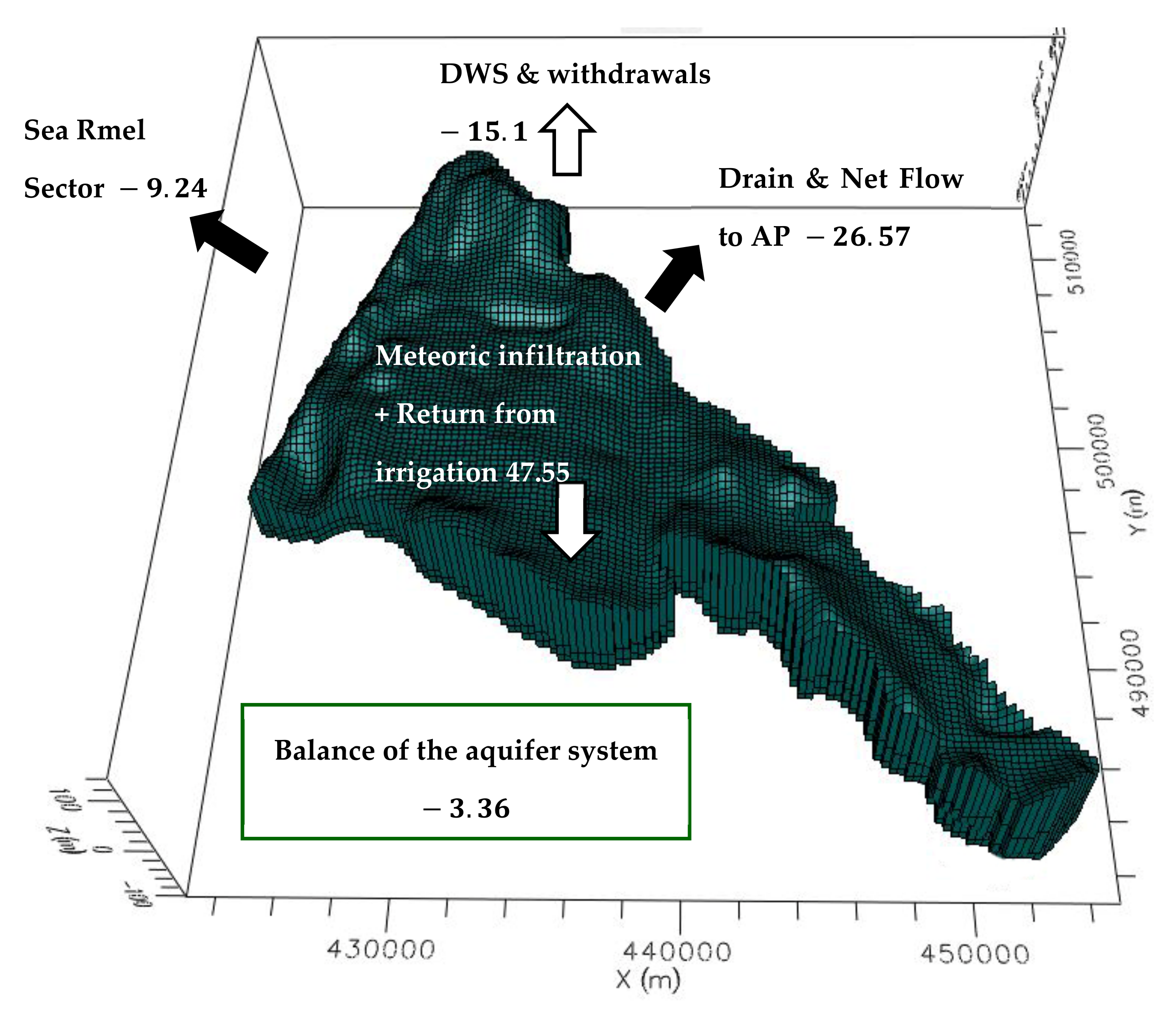
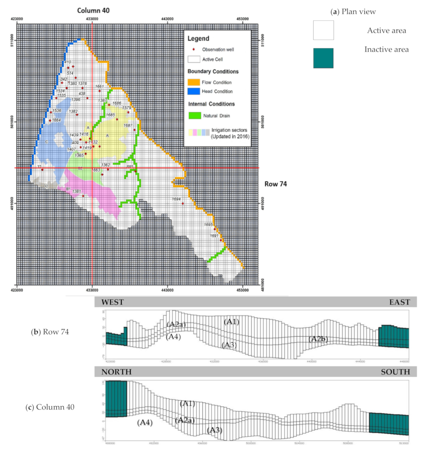
For this purpose, the study’s goals are to (i) describe and characterize the case study (e.g., geography and climate) (Section 2.1); (ii) define the geological and hydrogeological setting of the study area (Section 2.2 and Section 2.3); (iii) understand the hydrodynamic functioning of this hydrogeological system by quantifying the components of the GW mass balance (Section 2.4); (iv) design a conceptual model of the ROOCA (model set-up, initial and boundary conditions, model calibration and validation, time step of the simulations, the distribution of recharge from all sources and pumping, etc.); (v) design a computational model for simulating saltwater intrusion in the ROOCA using SEAWAT code; and (vi) determine the expected future forcing on the ROOCA aquifer due to population increase, water demand (over-pumping), CC (rainfall reduction), and SLR extrapolations to assess the water balance terms and SWI volumes under CC scenarios (Section 3).

2. Materials and Methods

2.1. Description of the Site

The study site (ROOCA) can be considered representative of the majority of northern Moroccan seashores. It is located in the northwestern part of Morocco in the low Loukkos basin immediately south of Larache city, with an area of about 305 km² (Figure 3). This region is bounded to the west by the Atlantic Ocean along a 20 km band, a succession of hills of Prerifan geological formations to the east, Mio-Pliocene marl outcrops to the southeast, and a risen bottom that acts as a water divide line between the ROOCA and the Dradere-Soueire aquifers to the south [48]. Figure 4 depicts that ROOCA areas are home to more than 4.5 million people. The observed increase in the urban population is attributable to natural demographic growth and the rural exodus from rural to urban space, as well as the formation of new urban centers and the expansion of city borders.

The Atlantic Ocean influences the region’s climate, which is subhumid. The monthly temperature values in the Loukkos basin show an increase over the last three decades, dating back to 1976 (Figure 5a). The annual average temperate in July to January ranges from 25.05 to 12.18 °C. State annual rainfall recorded from 1961 to 2016 is around 684 mm. Figure 5b shows a clear seasonal irregularity, where the ombrothermic diagram shows that the majority of the rainfall falls from October to March, with the rest of the year being almost completely dry (Figure 5d). In the study region, the yearly average evapotranspiration is calculated to be 384 mm/year. An influence of CC in the Loukkos basin triggers recurring droughts and reductions in recharge (Figure 5c). This is coupled with EOP (Figure 5e) to supply industrial and domestic irrigation and agricultural and metropolitan regions. The whole state has experienced a significant decrease in GW level (Figure 5f), which could potentially result in an aquifer water balance deficit and a loss of GW production due to SWI on the study area’s coast and coastal plain.

2.2. Geological Background

The existing geologic units in the research field have been intensively studied [50,51,52] (Figure 6a). The geological framework of ROOCA is characterized by the Pliocene–Quaternary superposition above a regional, Mio-Pliocene, predominantly marly, layer. It is formed from the bottom to the top by the following layers: (1) The Mio-Pliocene sediments are marked by blue marls, which form the impermeable bedrock of the aquifer. (2) The Plio-Villafranchian sediments are characterized by coastal and dune deposits that are usually 20 to 50 m thick and are composed of shelly sandstones, sands, and sandy marls. The continental deposits of the Villafranchian period are composed of red-clay cement pebbles surrounded by red sandy clays. (3) The Quaternary: Sandstones and coquina are marine Quaternary remains (ancient Quaternary). Rhamna sands and dune sandstones, as well as numerous fluviatile alluvial deposits, comprise the continental Quaternary and sandstones. The most recent Quaternary alluvial deposits (which contain some blue marls that are more or less sandy and contain marine shells, attributed to the Flandrian transgression) contain primarily red clays with sandy or stony passages, attributed to the Soltanian, and marl–silty layers that are black or greyish, attributed to the Rharbian.

This zone was very sensitive to Post-Villafranchian tectonic movements; they isolated the low Loukkos basin to the north and the Dradere-Souere basin to the south. The structure is characterized by NW–SE orientated ripples showing basins (Rhamna) separated by anticlines (Figure 6a).

2.3. Hydrogeology

For the hydrogeological background, Rmel coastal aquifers are made up of Plio-Quaternary sands and sandstone, but the bottom is composed of blue marls [52]. ROOCA is made up of Moghrebian [53] shelly sandstones that are topped in the Rmel field by Quaternary sands and marly red silts. In the Oulad-Ogbane region, they grow sideways in pebbles and coarse silt. Its thickness varies between 0.1 and 146 m. ROOCA’s thickest coat is found in a large bowl of Rhamna (140 m), which gradually reduces closer to the edges. The isopach map of the intermediate layer, which comprises clayey soil and sandy clay in the Rmel zone, forms a semipermeable screen that hydraulically isolates the two aquifers (upper and lower) [54]. The ROOCA aquifer is partly confined (limited) and partly unconfined for the rest of the area. These field observations have been taken into account when modeling the aquifer; they are based on pumping test measurements (DRPE, 1987) and show (1) existence of a limited “semiconfined” area with a constant delayed flow (leakage) and (2) existence of an unconfined area with a nonconstant delayed flow. Three geological cross-sections are given and illustrate more details of the existing hydrogeological units:

• Segment No. 1 of the hydrogeological cross-section (Figure 6b), located at the north of the Rhamna Basin, is in the axis of the opening of this basin on the sea. In the 305/3 borehole, the bottom is at −40 m altitude. The synclinal bowl elongated along the sea has an opening on the sea and the basin. Boreholes 428/3, 306/3, and 305/3 are sufficient to eliminate any ambiguity on this subject. Towards the west, the red silts disappear and give way to wind sands and dunes.
• The hydrogeological cross-section No. 2 (Figure 6b) directed SW–NE demonstrates that borehole 495/3 shows the divergence of the Rhamna basin on the left from the ocean on the west. The raising of the marly bottom has resulted in the separation of these two basins.
• Section No. 3 of the hydrogeological system (Figure 6b) is situated in the north–south direction. The Rhamna field is intersected by the profile between Larache and Laouamra (Figure 6a). There are two distinct parts: a Rhamna basin in the north and an expanded bowl of pebbles in the south. At Larache, the bedrock is at a depth of +20 m and drops to −77 m in the middle (borehole 86/3). Due to Post-Villafranchian erosion, the shell sandstones vanish at borehole 30/3. Boreholes 30/3 and 701/3 were packed with alluvial deposits and aeolian sands. Shell sandstones resurface in the boreholes 470/3, 700/3, and 704/3 but are missing in borehole 705/3, where the Villafranchian pebbles are found above the Pliocene marl sands [51].

In this analysis, we attempted to model the subsurface of this region in a geoscientific information system (GSIS) using the RockWorks program and borehole data. This program was designed for data collection, viewing, and analysis and displays the reservoir’s hydrogeological composition, extension, and geometry (Figure 7). This software platform is used for incorporating 3D geological models of sedimentary media into traditional hydrogeological modeling methods.

The 127 complete boreholes georeferenced in GIS were integrated into the RockWorks ‘Borehole Manager’ module that contains borehole processes such as data entry, management, and review (Figure 7a). The location of these boreholes is illustrated in Figure 7b. The geological units encountered are explicitly mentioned in the geometric model, as shown in Figure 7b–d below. The ‘Stratigraphy model’ module of RockWorks was used to convert all boreholes data and cross-sections into a 3D model representing the geometric model as a whole. The program creates a grid pattern of each surface and its stratigraphic base. The 3D solid allowed us to determine the geometry, volume, and location of lithostratigraphic deposits in the GW environment of the ROOCA (Figure 7c), and the fence diagram visualizes the configuration between overlapping surfaces (Figure 7d). Additionally, a geostatistical analysis was performed, and some prediction maps were incorporated into the three-dimensional geoscientific information system (3D GSIS). For each measure, the normality test and pattern analysis were used to pick the relevant semivariogram and cross-validate the results [55].

This 3D modeling allowed the design of a conceptual model of the aquifer reservoir, the performance of a set of simulations of GW flow in steady and transient states, and the design of a solute transport model for SWI in the ROOCA.

2.4. Water Balance

The regional GW flow is primarily SW–NE, with discharge to the Atlantic Ocean. However, as a result of GW during pumping, a cone of depression shifts the flow pattern to the north. Variations caused by surface water recharge from irrigation and pumping wells can be seen in piezometric data records from 1980 to 2016. The largest renewable groundwater recharge source comes from rainfall and drainage return discharge. Based on a field investigation conducted in 2013/14, the overall GW withdrawal from the pumping wells is evaluated to be 479 L/s; recharge to the aquifer is predicted to be 1508 L/s (

Table 1. Water balance of ROOCA for the hydrological year 2013/2014.

Inflows	Q (L/s)	Q (m3/year)	Outflows	Q (L/s)	Q (m3/year)
Input			Pumping
Rain infiltration (area = 305 km2)	1139.2	35,928,965	- Rural DWS	18.3	576,480
Return from irrigation	329.6	10,394,266	- Urban DWS ONEE	185.3	5,844,252
Return from pumping irrigation	39.1	1,233,463	- Urban DWS RADEEL	71.8	2,264,700
			- Irrigation pumping	195.6	6,167,314
			- Industrial pumping	7.8	245,518
			Natural flow
			- To ocean	293.2	9,246,355
			- Rivers, springs, and swamp	292.5	9,224,911
			- To alluvial plain (AP)	550.0	17,346,061
Total	1508	47,556,693	Total	1615	50,915,176
Input–Output			−107	−3,358,482 m3/y

DWS: drinking water supply; ONEE: National Office of Drinking Water; RADEEL: Autonomous Intercommunal Board of Water and Electricity Distribution.

). In 2013/14, the expected outflow to the Atlantic Ocean is 293 L/s. According to the results of a hydrogeochemical analysis conducted between 1985 and 1992, GW salinity in certain coastal observation wells, where measurements were made between the water table level and the aquifer bottom, ranges from 1 to 6 g/L.

The development of a GIS database [56,57] helped to improve and update the ROOCA’s hydrogeological water balance based on a mass-balance model with respect to 1963 and 2014 (Table 1 and Figure 8). This was based on a global and comprehensive inventory of all pumping points (wells, boreholes, and springs) and rain data that are reasonably reliable to estimate lateral flow in 2013/14. Natural GW recharge was calculated using the disparity between inflows (rainfall, irrigation) and outflows (plant evapotranspiration, surface run-off, and drinking water supply (DWS)) in a soil water balance equation, as follows:

• Calculation of GW recharge indirectly;
• Assessment of GW withdrawals for rural, DWS, and industrial purposes using indirect calculation or data collection;
• Calculation of aquifer inflow and outflow values for nearby water sources.

2.5. Conceptual Model

2.5.1. Model Discretization

Using the database developed by [56,57], the mathematical model developed simulates transient GW flow and solute transport for variable density from 1962 to 2040.

The model grid in the plan view is made up of 128 columns and 128 rows of 250 m (NS direction) and 250 m (S direction) with uniform spacing (WE direction), in that order (Figure 9a). The model grid, vertically oriented, is made up of three-layer construction that corresponds to the above-mentioned ROOCA hydro-stratigraphy layers (Figure 9b,c). The cross-section through the Rmel coastal plain, as well as the hydrogeologic units and a vertical view of spatial discretization for the quasi-three-dimensional numerical model, is shown by the red line. An inactive area is represented by the green color, while the active area is represented by the white color.

The Quaternary aquifers are represented by Layer A1. Layer A2a is an established aquitard between layers A1 and A3 of the Rmel aquifer, and it is thought to be semi-impermeable. When the thickness of Layer A2a exceeds 30 m, Layer A3 reflects the Moghrebian aquifer, which acts as a semiconfining to confining layer. In the Oulad-Ogbane sector, layer A2b represents pebbles and sandy silt. The bottom boundary (A4) in this model is set to Mio-Pliocene. The thickness of the model layer is calculated by (i) the presence of sand and shelly sandstone deposits documented in well driller’s documents archived at the Loukkos Hydraulic Basin Agency (ABHL) and the Direction of Water Research and Planning (DRPE) and (ii) a 3D GSIS (Figure 7), which depicts the reservoir’s hydrogeological composition, expansion, and geometry. The model simulation used a total of seven stress periods, ranging from 1961/1962 to 2039/2040, with a one-year time step.

2.5.2. Parameters in Hydrogeology

The hydraulic conductivity distribution was determined using data from pumping tests conducted at the time of good completion and recorded in well driller logs [54]. Each zone’s hydraulic conductivities are standardized. Pumping tests yielded hydraulic conductivities ranging from 9 × 10⁻⁵ to 2.2 × 10⁻⁴ m/s. For model calibration, the hydraulic conductivities of the model were modified during model tuning to account for the scale of the field. The ABHL administration provided monthly precipitation data. Using the Thornthwaite method, we determined an average evapotranspiration rate of 383.7 mm/year. As a starting point, effective porosity of between 0.15 and 0.25 was chosen. The dispersion coefficients were calculated using a widely used approach based on the sample area’s scale [58]. The longitudinal dispersivity was set to 10 m. The ratio of horizontal transverse dispersivity to longitudinal dispersivity $({\mathsf{\alpha }}_{\mathrm{T}}/{\mathsf{\alpha }}_{\mathrm{L}}$) was thought to be about 0.01. However, it was believed that the vertical transverse dispersivity to longitudinal dispersivity ratio (${\mathsf{\alpha }}_{\mathrm{V}}/{\mathsf{\alpha }}_{\mathrm{L}}$) was 0.001. The sample region’s aquifer property values were assigned to the model cells (

Table 2. Aquifer parameters used for the study area.

Hydrodispersive Parameters	Unit	Value
Porosity	-	0.25
Longitudinal dispersivity	m	10
${\mathsf{\alpha }}_{\mathrm{T}}/{\mathsf{\alpha }}_{\mathrm{L}}$	-	0.01
${\mathsf{\alpha }}_{\mathrm{V}}/{\mathsf{\alpha }}_{\mathrm{L}}$	-	0.001

). The calibration of the model was completed to achieve findings that were as close to the observed concentration data as possible.

2.5.3. Initial and Boundary Conditions

Since the model was designed to simulate SWI into aquifers, both GW flow and solute transport processes were coupled at the same time, with initial and boundary conditions taken into consideration. The initial head values are set to grid top elevation and turned on in the MODFLOW/SEAWAT program. Moreover, the SEAWAT program was used to simulate the model in steady state over a 100-year period in order to calculate the initial concentrations of SWI in 1961. This result will be assigned as the initial concentrations for the transient state. For the flow computation, the boundary conditions (Figure 9a) were set as a constant head boundary with a blue line. Around the Atlantic coast, the cells have a persistent head (mean sea level). A no-flow boundary was established through marl outcrops to the southeast of ROOCA and by the risen bottom to the south, which serves as a dividing flow line between ROOCA and the Dradere-Souiere aquifer. A flow boundary was established in the rest of the aquifer (orange color) based on the observed data. The drain boundary is defined as a green line. The aquifer has internal hydrological stresses which are applied for the subsequent layers. The aquifer bottom has a no-flux boundary, while the aquifer top has a recharge boundary (rain and irrigation return flow). The cells along the Atlantic coast are given a specific concentration of 35 kg/m³.

2.5.4. Climate and Sea Level Data

Datasets used for this assessment comprise a combination of regional climate modeling projection data generated from Regional Initiative for Assessing Climate Change Impacts on Water Resources and Socioeconomic Vulnerability in the Arab Region (RICCAR) [59] and a set of local observation datasets for precipitation and temperature relevant to our study area. This section is based on extracting time series of Pr (Precipitation) and Ta (Temperature) variables for the entire time period from 1951 to 2100. The available files in the NetCDF format (.nc) were used to extract these time series for our study area located at latitude = 35.2° North and longitude = 6.16° West.

Based on RICCAR data, we could present some plots of time series that summarize and show the updated knowledge on the climatology of the study area. We have extracted climate data and plotted some diagrams in Figure 10 and Figure 11, which show the evolution of projected P and T for various climate models and scenarios. The main trends of the parameter variation are also provided to analyze and measure the CC tendency of these parameters. Temperature and precipitation projections are derived from CNRM-CM5, EC-EARTH, and GFDL-ESM2M regional climate models (RCMs) under Representative Concentration Pathway (RCP) 4.5 and RCP 8.5 scenarios. In all cases, the forecasts for these three RCM models indicate a drop in precipitation (Figure 10) and a rise in temperature (Figure 11). The main trend for RCP 8.5 is relatively much stronger, as temperature increases more and precipitation decreases more. Hence, CC surely will harm the aquifer recharge and SLR, which may pollute fresh GW coastal areas and reduce their potential recharge.

Based on National Oceanic and Atmospheric Administration (NOAA) data, the following figure (Figure 12) is plotted and provides time series for estimates of SLR based on measurements from satellite radar altimeters such as TOPEX/Poseidon (T/P), Jason-1, Jason-2, and Jason-3, which have been in use since 1991. Glacial isostatic change impacts on the geoid, which are estimated to be +0.2 to +0.5 mm/year when globally combined, are not included in the SLR calculations.

For our study area, we then deduce that the sea level will rise from ~29.71 mm by 2010 to ~71.72 mm by 2020 (Figure 13). The impacts of climate-induced SLR will become more evident as the severity of the phenomenon grows, especially in low-elevation coastal zones. Besides, the impact of CC (projected temperature and precipitation obtained from RCMs under RCP 4.5 and RCP 8.5 from 2020 to 2100) will have a negative impact on SLR in the study as a result of the melting of glaciers and the warming of the oceans. For this purpose, linear regressions were used to project SLR (yearly values) from 2020 to 2040 from the observed data in answer to the melting of glaciers and the warming of the oceans. This modification of SLR is implemented in our modeling step of GW flow and SWI into the aquifer.

2.5.5. Numerical Model

The GW numerical flow design was created based on using the finite difference method in Visual MODFLOW Flex and includes MODFLOW code [60,61]. In two- and three-dimensional problems, modular finite difference is used in (3D) modeling to solve the differential equation that regulates flow in a porous medium using the GW structure in steady and transient states of the ROOCA.

A 3D numerical GW flow model, calibrated under steady and transient states resolving Equation (1) [61] for the years 1962 to 2040, was elaborated using Visual MODFLOW.

$$\frac{\partial }{\partial \mathrm{x}}\left({\mathrm{K}}_{\mathrm{xx}}\frac{\partial \mathrm{h}}{\partial \mathrm{x}}\right)+\frac{\partial }{\partial \mathrm{y}}\left({\mathrm{K}}_{\mathrm{yy}}\frac{\partial \mathrm{h}}{\partial \mathrm{y}}\right)+\frac{\partial }{\partial \mathrm{z}}\left({\mathrm{K}}_{\mathrm{zz}}\frac{\partial \mathrm{h}}{\partial \mathrm{z}}\right)\pm \mathrm{W}={\mathrm{S}}_{\mathrm{s}}\times \frac{\partial \mathrm{h}}{\partial \mathrm{t}}$$

(1)

where K_xx, K_yy, and K_zz are the K-values along of the x, y, and z align directions (L/T); h is the hydraulic head (L); W is the volumetric flux per unit volume and represents sources and (or) sinks (T⁻¹); S_s is the specific storage of the porous medium (L⁻¹); and t is the time.

After that, a 3D variable-density GW flow model, calibrated under steady and transient states resolving Equation (2) for the years 1962 to 2040, was generated using Visual MODFLOW and the SEAWAT code [62,63], which is a valuable method for simulating different variable-density fluids moving through dynamic-geometry hydrogeological environments, such as SWI in coastal aquifers. SEAWAT was created by integrating an updated version of MODFLOW with MT3DMS in a single programming application.

As flow and transport are inextricably linked, they were used to study SWI in the ROOCA under a distribution of salt concentration values in the coastal area.

$$\frac{\partial \mathrm{C}}{\partial \mathrm{t}}=\frac{\partial }{\partial {\mathrm{x}}_{\mathrm{i}}}\left({\mathrm{D}}_{\mathrm{ij}}\frac{\partial \mathrm{C}}{\partial {\mathrm{x}}_{\mathrm{j}}}\right)-\frac{\partial }{\partial {\mathrm{x}}_{\mathrm{i}}}\left({\mathrm{V}}_{\mathrm{i}}\mathrm{C}\right)-\frac{{\mathrm{q}}_{\mathrm{s}}{\mathrm{C}}_{\mathrm{s}}}{\mathsf{\theta }}+{\displaystyle \sum }_{\mathrm{k}=1}^{\mathrm{N}}{\mathrm{R}}_{\mathrm{k}}$$

(2)

Here, C is the contaminant concentration in GW (ML⁻³), x_i is the position in the cartesian coordinate axes (L), D_ij is the hydrodynamic dispersion coefficient (L² T⁻¹), V_i is the fluid velocity (LT⁻¹), q_s is the flow per unit of injected aquifer length (or pumped), Cs is the concentration of recharge or discharge flow (q_s) (ML⁻³), θ is the porosity of the porous medium, and Rk (k = 1,…,N) is the rate of solute production or decay in reaction k of N different reactions (M L⁻³ T⁻¹).

3. Results and Discussion

3.1. Calibration and Model Results

The main aim of the calibration stage is to produce results that are as close to the field data as possible by modifying the system’s parameters. Calibration of the model was accomplished by changing the distribution and values of two main parameters, namely the hydraulic conductivity and the specific storage coefficient of the aquifers. The hydraulic heads were determined by the model until they reach a suitable accuracy to match the observed values.

At first, the model was used in steady-state conditions for its calibration using observed piezometric data from 1961/62 [51]. The few known hydraulic property values were used as input parameters, and simulations were run by adjusting the hydraulic conductivity to obtain the best match between predicted and calculated piezometric values at the available control observation wells.

Following that, the PEST software was used to configure the model’s parameters and obtain optimal calibrations for various starting conditions. As seen in Figure 14a,b, the results indicate satisfactory agreement between computed and observed heads.

Figure 14b shows the good match between measurements and calculations in the 24 observation wells within the modeled region; the model calibration yielded two sets of values that are highly correlated, as illustrated by the map, which is very similar to the perfect correspondence axis in the scatter diagram, with an average correlation coefficient of 0.999, a mean error of 0.19 m, and a root mean square error of 0.849 m. The mean percentage difference is about 0.827 m, which is a reasonable value given that the computational model cannot account for local differences in the real world, and hydraulic head values were measured using altimetry data collected on a 1:50,000 scale (regional technical cartography). However, this means that the measured and computed heads are relatively similar. The overall model is then closer to reality, with respect to gradients and heads that are almost identical. The residuals between the observed and estimated heads are also indicated in

Table 3. Comparison of observed and calculated heads after calibration in 1961/1962.

Well ID (IRE/3)	X-Model	Y-Model	Heads Observed (m)	Heads Calculated (m)	Head (m)
336	432,350	506,350	11.46	11.29	0.17
342	429,950	505,850	3.63	3.75	−0.12
345	432,500	509,450	6.20	6.04	0.16
346	428,875	493,650	79.85	81.69	−1.84
348	437,525	494,150	38.00	36.52	1.48
355	431,925	507,475	13.84	14.15	−0.31
416	434,260	505,650	9.87	9.78	0.09
498	433,080	495,275	59.00	58.69	0.31
515	431,125	506,575	7.53	8.40	−0.87
601	433,225	501,800	14.10	13.06	1.04
605	428,950	503,850	2.50	4.22	−1.72
701	442,300	493,075	30.00	28.94	1.06
704	449,075	486,975	19.16	19.95	−0.79
730	430,225	508,175	1.28	2.65	−1.37
76	439,250	499,275	8.19	7.77	0.42
77	436,600	498,850	23.00	23.20	−0.20
84	436,900	500,075	16.41	17.99	−1.58
85	436,250	499,700	20.57	21.56	−0.99
86	435,750	498,600	25.63	26.95	−1.32

. The lateral hydraulic conductivity of layers A1, A2, and A3 as a result after model calibration varied from 4.10⁻⁴ to 8.10⁻⁷ m/s (Figure 15b).

The cross-sections and 3D representation of the stratigraphic model indicated the various aquifer levels (hydrogeological units) based on three geological ages ranging from the Plio-Quaternary to the Moghrebian aquifer. However, the lithostratigraphic formations are heterogeneous, varying in each unit where sands, marls, and silts (e.g., upper unit) can be found, which is why the Plio-Quaternary aquifer formation has 11 categories of permeabilities (

Table 4. Values of hydraulic conductivities before and after calibration in m/s and m/day.

K before Calibration		K after Calibration
m/s	m/day	m/s	m/day
0.00001	0.9	0.0000005	0.04
0.00003	2.6	0.0000008	0.1
0.00005	4.3	0.000004	0.3
0.00007	6.0	0.000005	0.4
0.00009	7.8	0.000008	0.7
0.00011	9.5	0.000025	2.2
0.00013	11.2	0.000025	2.2
0.00015	13.0	0.000035	3.0
0.00017	14.7	0.000101	8.7
0.00019	16.4	0.00025	21.6
0.00022	19.0	0.0004	34.6

). Hence, the hydraulic conductivity varies to account for the lithostratigraphy of the geological formations.

In the ROOCA aquifer, a geostatistical approach was used to study the spatial distribution of regionalized variables based on the pumping test data [55]. This K-value distribution was taken as initial values assigned to the model (initial permeability) and could not produce a simulated piezometry comparable to the measured one (1961/62). To overcome this situation, we used the K-value distribution based on earlier research conducted by Larabi on the same case study [64].

Table 5. Simulated and calculated water balance in steady state (the year 1963).

	Water Balance Component	Simulated	Calculated	Simulated	Calculated	Error		96% of inflows
		(in m3/day Volume)	(in m3/day Volume)	(Flow Rate in L/s)	(Flow Rate in L/s)
Inflows	Recharge by precipitation	163,080	163,080	1888	1888	0
	Return from irrigation	5910	5910	68	68	0
	Total	168,990	168,990	1956	1956	0
Outflows	Domestic water supply	24,659	24,659	285	285	0		56% of outflows
	Sea outflow	48,432	50,475	561	584	−0.040
	River drainage: Smid El Ma, El Kihel, Sakh-Sokh and alluvial plain	93,861	93,856	1086	1086	0
	Total	166,952	168,990	1932	1956
Error		0.0122	0

shows the observed and calculated water balance with its various elements, along with the release to shore, which is found to be 584 L/s. The key input variable is precipitation recharge, which represents 96% of inflows, and the main output component is drainage to rivers and towards the neighboring alluvial plain, which represents 56% of outflows.

However, in a transient state, the model was calibrated until the end of 2009 due to a lack of consistently controlled hydraulic head performance using observed hydraulic heads from 1961/62. In total, 22 observed hydraulic head simulations were performed during calibration. Figure 16 depicts the observation wells and the calculation done for the target period of 1963–2016 (53 years). When a fair fit between the observed and measured heads was satisfactorily reached, model calibration was terminated. Because of the small number and length of the observation results, the model calibration in this analysis can be considered based on these available data. When more evidence on data becomes usable in the future, further model calibration can be applied and the model results can be improved.

Hence, the model was calibrated to work under transient state conditions. The simulation in this case computes piezometric surface variations over time; hence, the parameters involved in the temporal equation can be calibrated (either a specific yield or a specific storage). Aquifer boundary inflows (flux at the boundary, meteoric recharge) and outflows (withdrawals) were also assessed and analyzed. The goal was to replicate the piezometric oscillations found at the control points as accurately as possible during the measurement period. The reference period for transient simulations corresponds to the one when GW level measurements were made. The computed piezometric heads found in steady-state regime acted as the initial conditions. The model was set up with the initial concentrations of SWI in 1961/1962. The simulation lasted a total of 20,075 days, beginning in 1962 and ending in 2016.

These simulations make use of wells that pump water mostly used for irrigation and DWS. Irrigation started in 1981 and lasted until 2016; withdrawals differ over time and are allocated based on both climate conditions and piezometric variations. The Thornthwaite technique was used to assess the monthly infiltration value that was distributed evenly throughout the month based on the meteoric recharge from the effective monthly precipitation. After calibration, the adopted basic storage was estimated to be between 0.1 and 4%. The calibration findings in a transient state regime are presented in the plots (Figure 17), which compare observed and computed heads. For the simulation time under consideration, this distinction demonstrates adequate consensus between measured and computed heads in various observation wells. GW pumping produces a significant drop in the GW level (piezometers 342/3, 438/3, and 1380/3), while irrigation in 1981 results in an increase in the water level (piezometers 32/3, 1432/3, and 1685/3).

3.2. Water Budget from 1961 to 2016

We assessed the amounts of the water budget at both the model borders and inside the aquifer itself. The simulation shows the start of the SWI and its progression over time, the pollution concentration, the intruded SWI length, and other mass balance elements. The aquifer system has a negative balance of over 12 hm³ (approximately 33,000 m³/day) between 1961/62 and 2015/16. It is worth noting that this time was marked by lower-than-average meteoric recharge (−60%). The quantity of recharge (varies between 54 hm³ and 20 hm³) and the quantity of water crossing the alluvial plain (approximately 20 hm³ inflow and over 25 hm³ outflows) are the most interesting key components. The disparity (approximately 5 hm³) reflects the net outflow of GW into the neighboring alluvial plain, which happens mostly on the left bank of the Loukkos wadi, as well as the amount of water outflowing towards the Atlantic Ocean (about 11 hm³). Furthermore, the amount of GW pumping is approximately 20 hm³.

Figure 18a depicts time differences in groudwater flow for each part of the water budget; note that substantial meteoric infiltration occurs primarily in 1962, 1968, 1976, 1996, and 2009 and that the piezometric level was highly affected by this recharge during these times.

The GW balance between 1962 and 2016 indicates that the aquifer had more freshwater storage between 1962 and 1976 and a decrease in aquifer recharge associated with EOP occurring between 1980 and 1990. As a result, seawater moved inland in 1982 and 1991 (Figure 18b,c). It also demonstrates that a decrease in recharge and EOP, especially in 1998, 2004, 2011, and 2015, increased SWI, though less pronounced than the intrusion of seawater in 1982 and 1991. The areas that have been intruded are as follows: (1) Between 1976 and 2016, the SWI entered the first region west of the ONEE pumping wells. Following that, the invaded region stretched along the coastal line for about 6 km in length and 0.5 km in width (see Figure 18, the small orange frame). (2) The aquifer is contaminated in the NW coastal plain, where the toe extends some 0.5 km inland. The contamination of the aquifer is limited beyond these areas.

Hence, when seawater directly joins the aquifer environment, it allows the chemical composition of GW to deteriorate by SWI. The situation is exacerbated by the presence of seawater at some times of the year when the piezometric levels are lower. The SWI edge extended 0.5 km into the aquifer bottom. We also observe that SWI increased in the northwestern sector in 1991/92, owing primarily to (1) decreased recharge induced by CC and intermittent droughts and (2) overexploitation of GW by extensive pumping out from the aquifer system for the water supply of the city of Larache, rural areas, and irrigation.

3.3. Climate Change, Over-Pumping, and SLR Impacts

The density-dependent numerical model that was designed was completed to simulate the flow and transport from 2017 to 2040, based on climate projections and GW management scenarios established by the National Office of Drinking Water (ONEE) in 2016 and ranging from 2017 to 2040 to meet the future water needs of both urban centers, Larache and Ksar El Kebir cities. Climate projections, under RCP 4.5, indicate a temperature rise of about 0.45 °C and a 16.7% decrease in precipitation from 2016 to 2050. Furthermore, the sea level will grow from 7 cm in 2020 to 15 cm by 2040.

For a period of 24 years, three planning scenario schemes were employed to simulate future changes in drawdown and salinity concentrations (Figure 19). The first scenario assumes that the same conditions are maintained and that the aquifer pumping rate of approximately 21.52 hm³/year is maintained until 2040. Surface water or a desalination plant will meet the future increased water demand. The change in the aquifer’s GW quality is also examined in order to determine the area affected by SWI. The second scenario involves increasing pumping rates until 2040 to supply the growing water demand of the Larache population. The third scenario assumes that additional GW abstractions will be required until 2040 to supply the water demands of both urban centers, Larache and Ksar El Kebir. Figure 19 depicts the three pumping scenarios and their progression to 2040. The projected drawdown and seawater volumes intruding into the aquifer are depicted in Figure 20, Figure 21 and

Table 6. Water budgets of 1961 and 2016 and the projection of the aquifer balance for the year 2040.

	Water Balance Terms (hm3/year)	1961	2016	2040
Inflow	Storage	0.00	12.54	2.97
	Recharge from alluvial plain	19.36	20.49	4.73
	Seawater intrusion	0.06	0.34	3.25
	Return from irrigation	2.08	9.95	10.75
	Recharge by precipitation	53.93	20.47	16.02
	Total	75.42	63.80	37.72
Outflow	Storage	0.00	0.00	0.01
	Wells	14.65	21.52	34.72
	Discharge to alluvial plain	32.31	25.64	2.51
	Discharge to Atlantic Ocean	15.86	9.55	0.18
	Drainage by rivers: Oueds Smid El Ma-El Kihel-Sakh Sokh	12.47	7.01	0.22
	Total	75.29	63.72	37.62
Error %		0.132	0.081	0.099

.

Scenario 1, which assumes that the current pumping is maintained and future water demand will be provided by surface water or by a desalination plant, has less influence on the renewable resources and the water quality of the ROOCA. Indeed, from 2020 to 2040, we will note a drop in SWI volume (Figure 20b), which is directly related to an increase in hydraulic head (Figure 20a) due to increased predicted recharge from 2017 to 2040 in the study area. Figure 20c also demonstrates that the salinity concentration will be almost zero at piezometer 1380/3.

Scenario 2 depicts a significant increase in salinity in the northwestern area, closer to the shoreline. The maximum extent of SWI will increase to 3.5 km deeper in the aquifer. The SWI volume intruding into the aquifer continues to rise (Figure 20b), while the GW level continues to decline, reaching maximum values around -10 m (Figure 20a). In 2040, however, the seawater would not reach the first series of wells. At piezometer 1380/3, the salinity concentration is also projected to rise to reach values around 20 g/L (Figure 20c).

Scenario 3 is the pessimist one and also shows the predicted drawdown and saltwater extent in the aquifer by 2040 depicted in Figure 21. Note that sea salt concentration (35 g/L) is in red and freshwater concentration, almost 0 g/L, is in blue. There will be a greater decrease in hydraulic heads because of intensive pumping discharge to address the two cities’ water needs. Indeed, hydraulic heads will hit negative values of around −20 m in the main ONEE well field sector (Figure 20a), where the drawdown will rise by 25 m, which is a substantial increase. The aquifer is also contaminated by SWI in the coastal part’s northwest region, where the toe would reach about 5.2 km inland with an invaded area of about 31 km² (Figure 21a) and would reach high salinity (15–25 g/L) in Layer 3 (Figure 21b). As a consequence, seawater would reach seven observation wells (1534/3, 1535/3, 1536/3, 1380/3, 342/3, 1396/3, and 438/3) and four pumping wells (417/3, 419/3, 718/3, and 1737/3) gradually in 2040. The expected salinity, greater than 2 g/L, will be already reached in 2032 and will continue to increase up to 6 g/L in 2040 (Figure 20a). A comparison between the second and third scenarios indicates that the salinity is expected to rise by 2040 from 20 to 30 g/L at piezometer 1380/3 located 1.5 km away from the coast (Figure 20c).

4. Conclusions

GW is the important source of freshwater in the Rmel-Oulad Ogbane coastal plain in the low Loukkos basin in Morocco, where 98% of the domestic water, as well as the entire industrial water supply, is dependent on GW. Therefore, it is imperative to protect GW from SWI in this area. Hence, there is a need for tools that can guide and assist the manager in decision-making regarding the use, management, and planning of water resources. Currently, these decision support elements are provided by efficient technical tools such as GIS, geostatistical analysis, and conceptual and mathematical models, as developed in this research.

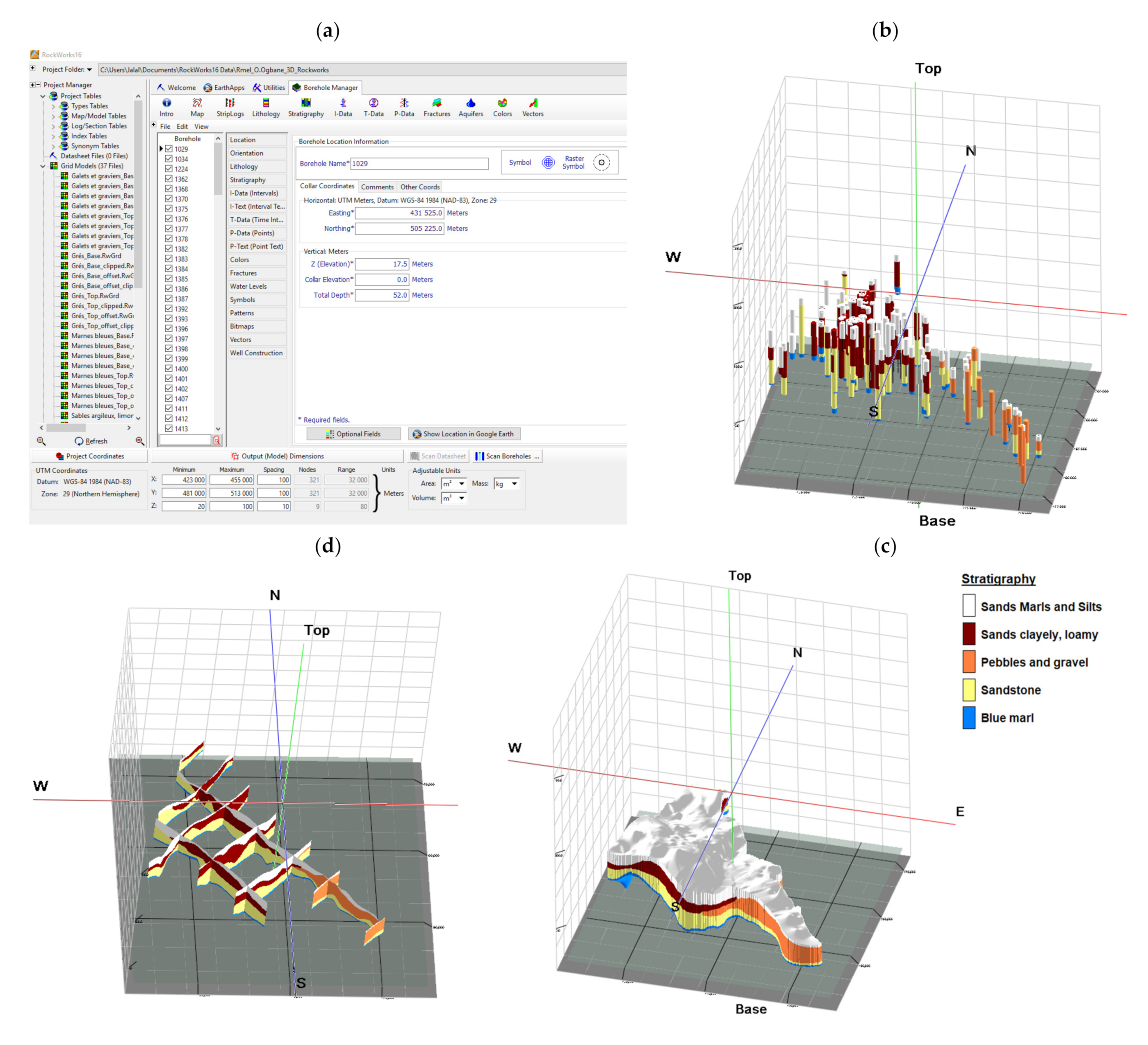
Using data from boreholes and hydrogeological investigations, we modeled the aquifer reservoir using a 3D GSIS. Then, a geostatistical model was produced from physicochemical, piezometric, and hydrodynamic parameters. These outputs were used to update the water balance in 2013/2014 and to develop a good conceptual model of the aquifer. Finally, to predict the current extent of SWI and provide useful information for the protection of GW resources, a three-dimensional numerical model of density-dependent GW flow and miscible salt transport of the subsurface aquifer was developed to assess the current extent of SWI in the study area with the aim of determining the impacts of CC due to increasing of temperatures, decreasing precipitation, and SLR during the 21st century. The developed model incorporated regional geologic, geographic, and hydrogeological features. The model input parameters were determined from analysis of well logs, well driller’s reports, and pumping tests. All these inputs were used to simulate three-dimensional variable-density GW flow under steady and transient states.

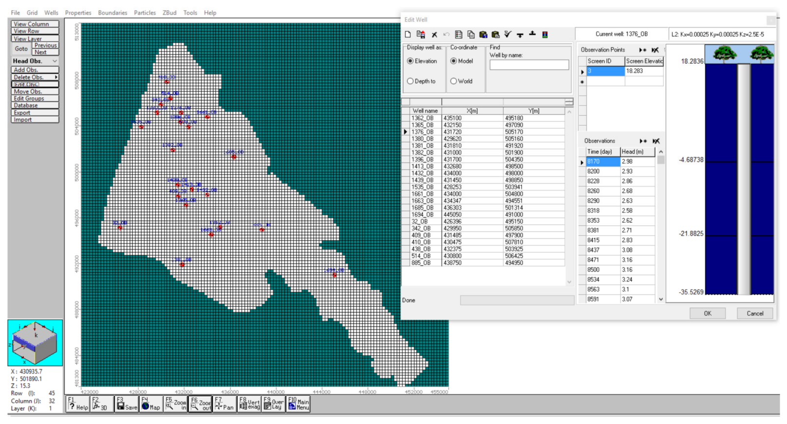
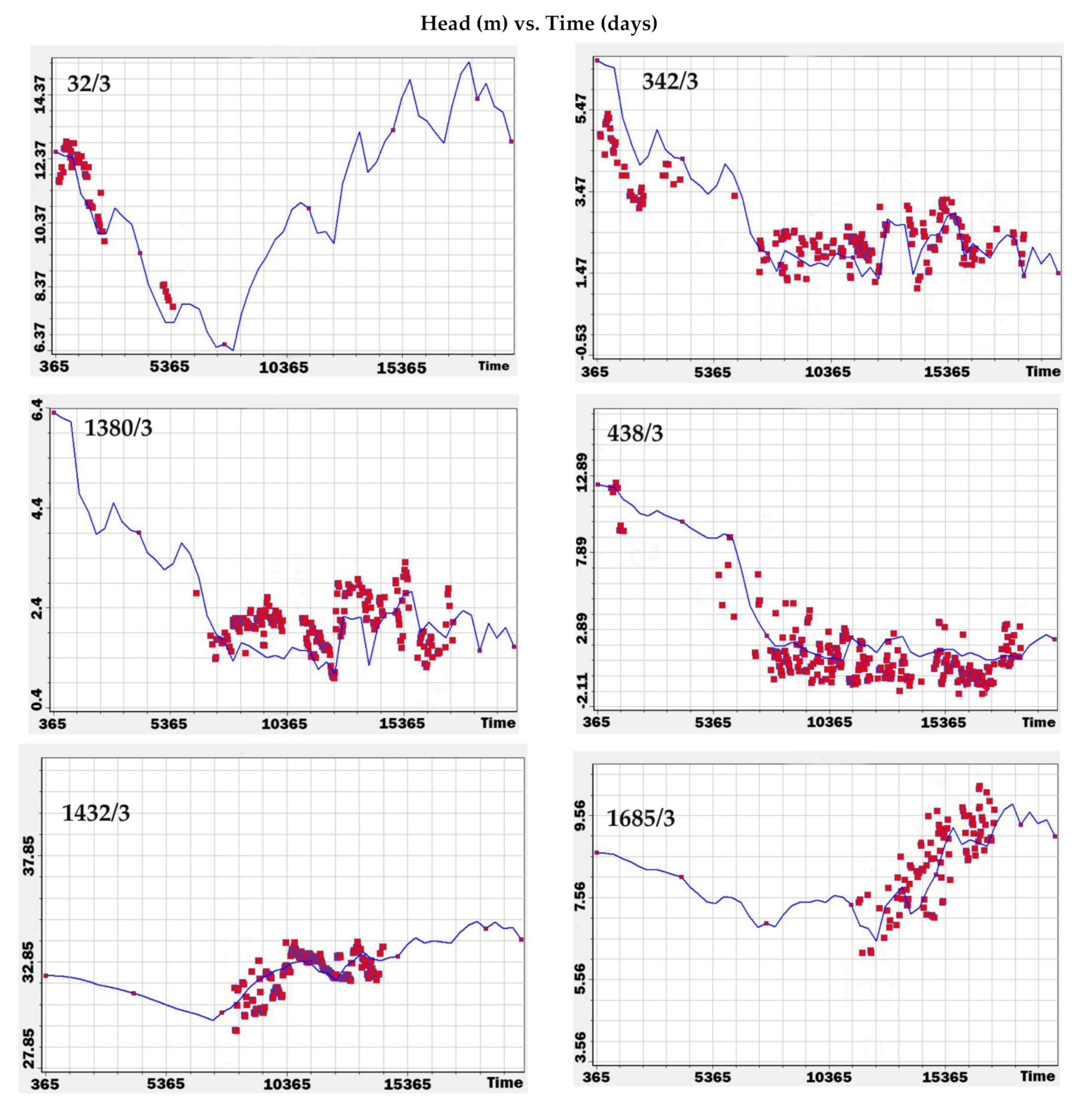
Due to the scarcity of some observed water quality data and continuously monitored head data, more field measurements, such as vertical salinity profile and trace element studies for dispersivity, need to be performed in order to improve the reliability of the model. For this performed calibration, a total of 22 observed hydraulic head values were used, resulting in good agreements between the observed and calculated hydraulic heads. When more data become available in the future, additional calibration would be needed. Moreover, an optimization model for rational management of the aquifer must be developed.

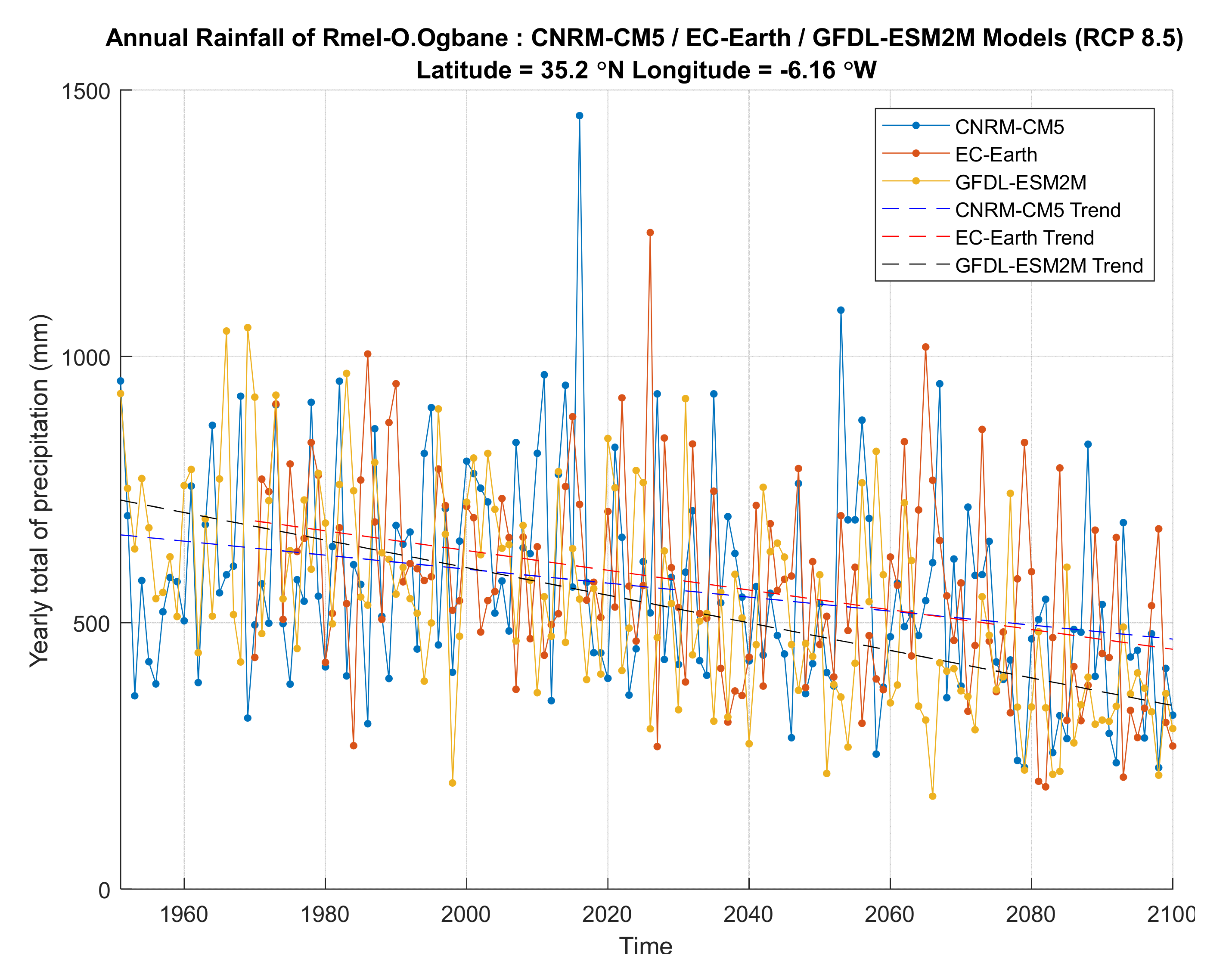
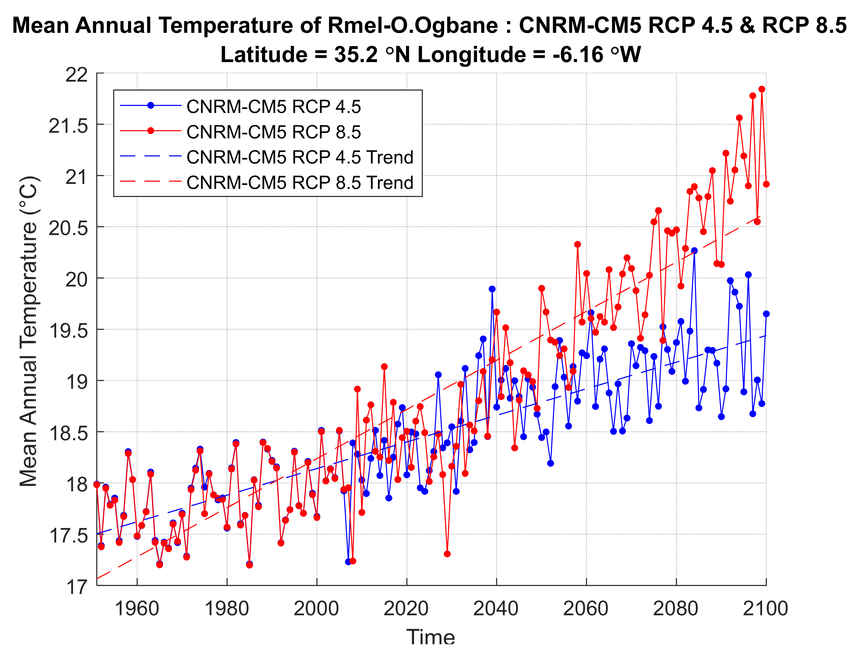
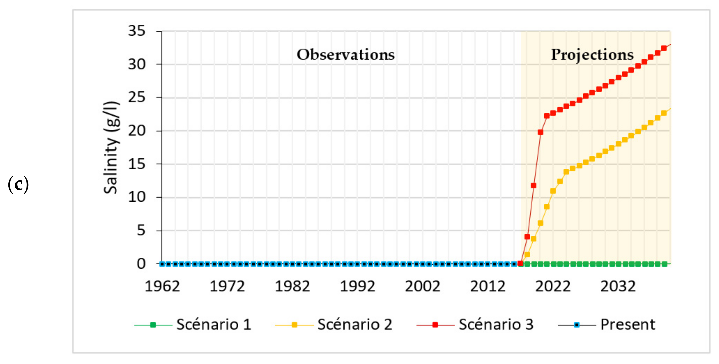
Climate projections used in this assessment comprise a combination of regional climate modeling projection data, generated from RICCAR, and a set of local observation datasets for precipitation and temperature for the study area. Projected temperature and precipitation were obtained from CNRM-CM5, EC-EARTH, and GFDL-ESM2M RCMs under RCP 4.5 and RCP 8.5 scenarios. These projections show a decrease in precipitation and an increase in temperature for both scenarios. As a result, CC would almost certainly have a detrimental effect on SLR, reducing the availability of new GW resources. The increase in sea level would affect coastal aquifers, shifting the saltwater interface farther inland. Indeed, the model took into account the predicted SLR and used it to adjust the boundary conditions.

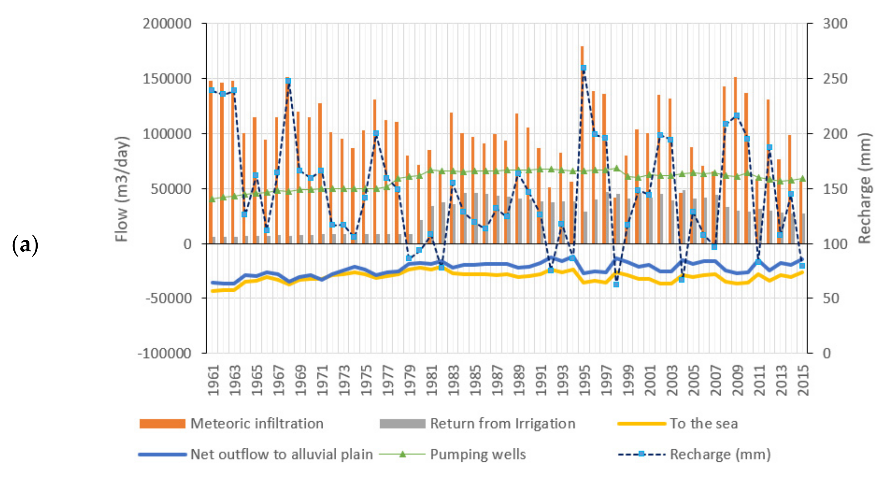
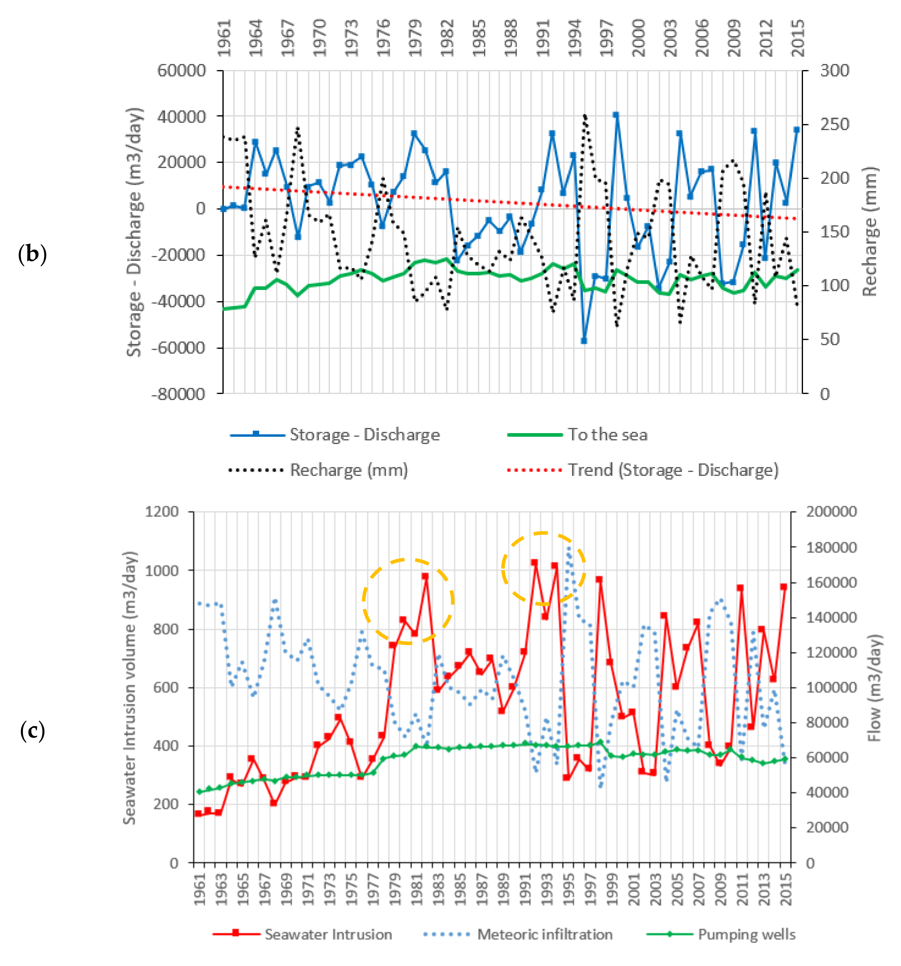
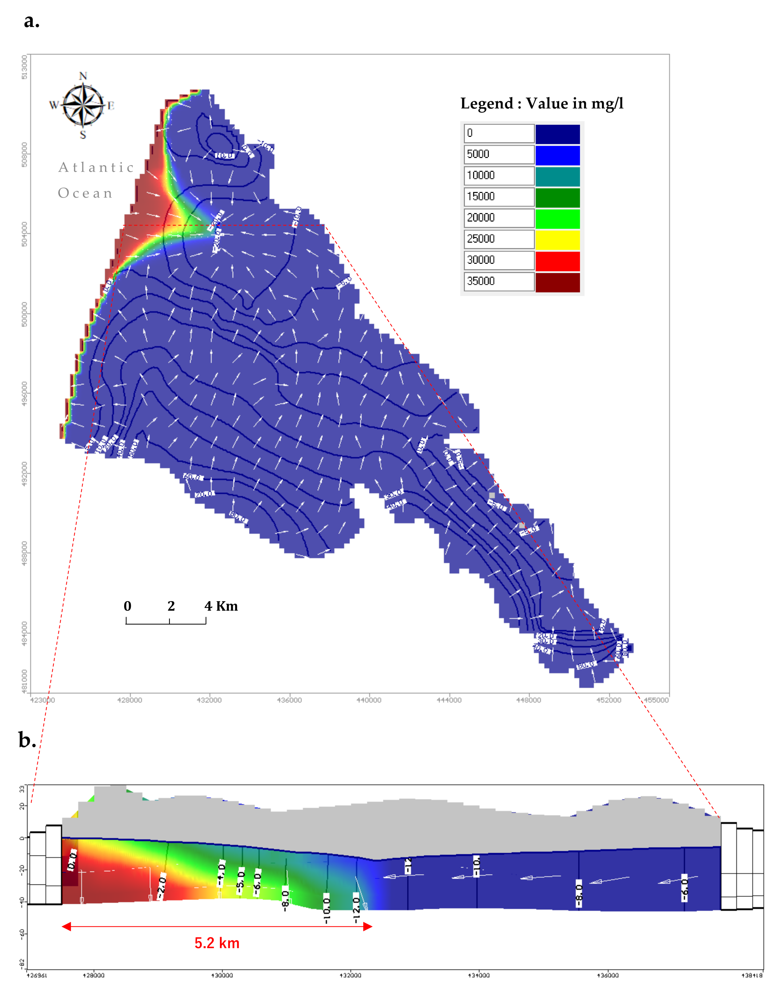
The variation in recharge was determined by taking into account the variations in return from irrigation and climatic parameters (precipitation and temperature). The numerical simulations were conducted for a period of approximately 76 years and dealt with SWI relating to GW abstraction, climatic parameters, and SLR. The simulation results under RCP 4.5 show that the maximum extent (about 5.2 km) of SWI would increase in 2040 in the northwestern sector of the study area. The water quality would be most affected in the ONEE pumping area, which is directly adjacent to the seashore. As a result, the GW abstraction associated with CC is the primary driver of SWI in the study area. Furthermore, the reduction in recharge and the rise in sea level caused by CC exacerbate saltwater intrusion into the aquifers, reducing the fresh GW resources.

The primary impact of this SWI in the ROOCA would be unnecessary over-pumping that would deplete renewable water resources. However, this situation can be improved by the use of surface water for irrigation (provided from the neighboring dam reservoir), a desalination plant project for DWS, and artificial recharge of the aquifer. GW recharge with recycled water would be also an effective and feasible way to address the rapid GW depletion and saltwater intrusion in the ROOCA. Recycled water is a sustainable and reliable source of local water that should be viewed as a valuable resource. Indeed, GW recharge is an excellent utilization of recycled water as it provides natural storage (which allows for drought mitigation or withdrawal when demand for water increases) and soil treatment (with surface spreading), and it can be used to directly prevent SWI (with a direct injection barrier, for instance). Thus, the city of Larache, which is located directly at the northern limit of the study site, has a good potential for wastewater to be produced for the artificial recharge of the coastal fringe of the aquifer, which is distinguished by sand dunes, very favorable to infiltration and natural purification.

This would greatly increase the GW production in the coastal sectors of the aquifer and would protect freshwater from SWI. Such long-term results and findings will help the local decision-makers and all relevant stakeholders to better plan, manage, and improve the fresh GW resources for the ROOCA.

Morocco has more than 3500 km of coastline (two maritime facades: Atlantic, 2,934 km; Mediterranean, 512 km) with several thousand hectares of coastal plains, where irrigated agriculture is well developed, such as in this case study, in addition to more industries and the most important cities in the country (Casablanca, Rabat, Tangier, Agadir, etc.). These coastal plains contain coastal aquifers that are overexploited and threatened by SWI. Some large cities are already supplied with surface water, GW, and desalination water (Agadir, Casablanca, Al Hoceima). Therefore, this study will serve as a pilot study in order to implement the established methodology. It is also recommended to complement this study with an in-depth study on the choice of artificial recharge sites and a study to optimize the management of conventional and unconventional water resources in order to minimize the energy costs associated with desalination and wastewater treatment, especially during wet and dry periods caused by CC.

It is also recommended to extend this established methodology to study further similar coastal aquifers abroad in terms of climate conditions, such as in the Mediterranean region, as this will help the decision-makers in water resources planning and development and securing sustainable GW management of the coastal aquifers. This methodology can be completed by an impact modeling study based on the application of artificial recharge (from available sources) in well-chosen sites in order to improve the production of water resources and limit the entry of seawater into freshwater of the coastal aquifer.

References

1. Oude Essink, G.H.P. Improving fresh groundwater supply—Problems and solutions. Ocean Coast. Manag. 2001, 44, 429–449. [Google Scholar] [CrossRef]
2. HCP Recensement Général de la Population et de l’Habitat (RGPH). Available online: http://rgphentableaux.hcp.ma/ (accessed on 8 February 2021).
3. Bouchaou, L.; Hsissou, Y.; Krimissa, M.; Krimissa, S.; Mudry, J. 2H and 18O isotopic study of ground waters under a semi-arid climate. In Environmental Chemistry: Green Chemistry and Pollutants in Ecosystems; Springer: Berlin/Heidelberg, Germany, 2005; pp. 57–64. ISBN 3540228608. [Google Scholar]
4. Boughriba, M.; Melloul, A.; Zarhloule, Y.; Ouardi, A. Extension spatiale de la salinisation des ressources en eau et modèle conceptuel des sources salées dans la plaine des Triffa (Maroc nord-oriental). C. R. Geosci. 2006, 338, 768–774. [Google Scholar] [CrossRef]
5. Zouhri, L.; Arbi Toto, E.; Carlier, E.; Debieche, T.-H. Salinité des ressources en eau: Intrusion marine et interaction eaux–roches (Maroc occidental). Hydrol. Sci. J. 2010, 55, 1337–1347. [Google Scholar] [CrossRef]
6. Najib, S. Etude de l’Évolution de la Salinisation de l’Aquifère de la Chaouia Côtière (Azemmour-Bir Jdid, Maroc): Climatologie, Hydrogéologie, Hydrochimie et Tomographie Électrique—Archive Ouverte HAL; Université Chouaib Doukkali: El Jadida, Morocco, 2014. [Google Scholar]
7. Gaaloul, N.; Cheng, A.H.-D. Hydrogeological and Hydrochemical Investigation of Coastal Aquifers in Tunisia-Crisis in Overexploitation and Salinization. In Proceedings of the 2nd International Conference on Saltwater Intrusion and Coastal Aquifers—Monitoring, Modeling, and Management, Merida, Mexico, 30 March–2 April 2003. [Google Scholar]
8. Kerrou, J. Deterministic and Probabilistic Numerical Modelling towards Sustainable Groundwater Management: Application to Seawater Intrusion in the Korba Aquifer (Tunisia). Ph.D. Thesis, Université de Neuchâtel, Neuchâtel, Switzerland, 2008. [Google Scholar]
9. Kouzana, L.; Benassi, R.; Ben Mammou, A.; Sfar Felfoul, M. Geophysical and hydrochemical study of the seawater intrusion in Mediterranean semi arid zones. Case of the Korba coastal aquifer (Cap-Bon, Tunisia). J. Afr. Earth Sci. 2010, 58, 242–254. [Google Scholar] [CrossRef]
10. Alfarrah, N.; Walraevens, K. Groundwater Overexploitation and Seawater Intrusion in Coastal Areas of Arid and Semi-Arid Regions. Water 2018, 10, 143. [Google Scholar] [CrossRef] [Green Version]
11. Antonellini, M.; Mollema, P.; Giambastiani, B.; Bishop, K.; Caruso, L.; Minchio, A.; Pellegrini, L.; Sabia, M.; Ulazzi, E.; Gabbianelli, G. Salt water intrusion in the coastal aquifer of the southern Po Plain, Italy. Hydrogeol. J. 2008, 16, 1541–1556. [Google Scholar] [CrossRef]
12. Paniconi, C.; Khlaifi, I.; Lecca, G.; Giacomelli, A.; Tarhouni, J. Modeling and analysis of seawater intrusion in the coastal aquifer of Eastern Cap-Bon, Tunisia. Transp. Porous Media 2001, 43, 3–28. [Google Scholar] [CrossRef] [Green Version]
13. Qahman, K.; Larabi, A. Numerical modeling of seawater intrusion in Khan-Younis area of the Gaza Strip Aquifer, Palestine. Dev. Water Sci. 2004, 55, 1629–1641. [Google Scholar] [CrossRef]
14. Gingerich, S.B.; Voss, C.I. Three-dimensional variable-density flow simulation of a coastal aquifer in southern Oahu, Hawaii, USA. Hydrogeol. J. 2005, 13, 436–450. [Google Scholar] [CrossRef]
15. Feseker, T. Numerical studies on saltwater intrusion in a coastal aquifer in northwestern Germany. Hydrogeol. J. 2007, 15, 267–279. [Google Scholar] [CrossRef]
16. Cobaner, M.; Yurtal, R.; Dogan, A.; Motz, L.H. Three dimensional simulation of seawater intrusion in coastal aquifers: A case study in the Goksu Deltaic Plain. J. Hydrol. 2012, 464–465, 262–280. [Google Scholar] [CrossRef]
17. Felisa, G.; Ciriello, V.; Di Federico, V. Saltwater Intrusion in Coastal Aquifers: A Primary Case Study along the Adriatic Coast Investigated within a Probabilistic Framework. Water 2013, 5, 1830–1847. [Google Scholar] [CrossRef] [Green Version]
18. Fahs, M.; Koohbor, B.; Belfort, B.; Ataie-Ashtiani, B.; Simmons, C.T.; Younes, A.; Ackerer, P. A Generalized Semi-Analytical Solution for the Dispersive Henry Problem: Effect of Stratification and Anisotropy on Seawater Intrusion. Water 2018, 10, 230. [Google Scholar] [CrossRef] [Green Version]
19. Abd-Elhamid, H.F.; Abd-Elaty, I.; Sherif, M.M. Effects of Aquifer Bed Slope and Sea Level on Saltwater Intrusion in Coastal Aquifers. Hydrology 2020, 7, 5. [Google Scholar] [CrossRef] [Green Version]
20. Gogu, R.C.; Carabin, G.; Hallet, V.; Peters, V.; Dassargues, A. GIS-based hydrogeological databases and groundwater modelling. Hydrogeol. J. 2001, 9, 555–569. [Google Scholar] [CrossRef]
21. El Idrysy, H.; De Smedt, F. Modelling groundwater flow of the Trifa aquifer, Morocco. Hydrogeol. J. 2006, 14, 1265–1276. [Google Scholar] [CrossRef]
22. Mondal, N.C.; Singh, V.S. Mass transport modeling of an industrial belt using visual MODFLOW and MODPATH: A case study. J. Geogr. Reg. Plan. 2009, 2, 001–019. [Google Scholar]
23. Toto, E.A.; Zouhri, L.; Jgounni, A. Modélisation directe et inverse de l’écoulement souterrain dans les milieux poreux. Hydrol. Sci. J. 2009, 54, 327–337. [Google Scholar] [CrossRef]
24. Green, T.R.; Taniguchi, M.; Kooi, H.; Gurdak, J.J.; Allen, D.M.; Hiscock, K.M.; Treidel, H.; Aureli, A. Beneath the surface of global change: Impacts of climate change on groundwater. J. Hydrol. 2011, 405, 532–560. [Google Scholar] [CrossRef] [Green Version]
25. Tramblay, Y.; Badi, W.; Driouech, F.; El Adlouni, S.; Neppel, L.; Servat, E. Climate change impacts on extreme precipitation in Morocco. Glob. Planet. Chang. 2012, 82–83, 104–114. [Google Scholar] [CrossRef]
26. Tramblay, Y.; Ruelland, D.; Bouaicha, R.; Servat, E. Projected climate change impacts on water resources in northern Morocco with an ensemble of regional climate models. In Proceedings of the FRIEND-Water 2014, Montpeiller, France, 7–10 October 2014; pp. 250–255. [Google Scholar]
27. Sahoo, S.; Jha, M.K. Modélisation numérique des écoulements d’eau souterraine pour évaluer les effets potentiels d’un pompage et de la recharge: Conséquences pour la gestion durable des eaux souterraines dans la région du delta de Mahanadi, en Inde. Hydrogeol. J. 2017, 25, 2489–2511. [Google Scholar] [CrossRef]
28. Hugman, R.; Stigter, T.; Costa, L.; Monteiro, J.P. Numerical modelling assessment of climate-change impacts and mitigation measures on the Querença-Silves coastal aquifer (Algarve, Portugal). Hydrogeol. J. 2017, 25, 2105–2121. [Google Scholar] [CrossRef]
29. El Mokhtar, M.; Chibout, M.; El Mansouri, B.; Chao, J.; Kili, M.; El Kanti, S.M. Modeling of the Groundwater Flow and Saltwater Intrusion in the Coastal Aquifer of Fum Al Wad, Province of Laayoun, Morocco. Int. J. Geosci. 2018, 9, 71–92. [Google Scholar] [CrossRef] [Green Version]
30. Abd-Elhamid, H.F.; Javadi, A.A.; Qahman, K.M. Impact of over-pumping and sea level rise on seawater intrusion in Gaza aquifer (Palestine). J. Water Clim. Chang. 2015, 6, 891–902. [Google Scholar] [CrossRef]
31. Ranjbar, A.; Cherubini, C.; Saber, A. Investigation of transient sea level rise impacts on water quality of unconfined shallow coastal aquifers. Int. J. Environ. Sci. Technol. 2020, 17, 2607–2622. [Google Scholar] [CrossRef]
32. Oude Essink, G.; Schaars, F. Impact of climate change on the groundwater flow system of the water board of Rijnland, The Netherlands. In Proceedings of the 17th Salt Water Intrusion Meeting, Delft, The Netherlands, 6–10 May 2002. [Google Scholar]
33. Tiruneh, N.D.; Motz, L.H. Three Dimensional Modeling of Saltwater Intrusion Coupled with the Impact of Climate Change and Pumping. In Proceedings of the World Water and Environmental Resources Congress, Philadelphia, PA, USA, 23–26 June 2003; pp. 1–9. [Google Scholar] [CrossRef]
34. Canning, D.J. Climate Variability, Climate Change, and Sea-Level Rise in Puget Sound: Possibilities for the Future. In Proceedings of the Puget Sound Georgia Basin Conference, Bellevue, WA, USA, 12–14 February 2001. [Google Scholar]
35. Yang, Y.; Song, J.; Simmons, C.T.; Ataie-Ashtiani, B.; Wu, J.; Wang, J.; Wu, J. A conjunctive management framework for the optimal design of pumping and injection strategies to mitigate seawater intrusion. J. Environ. Manag. 2021, 282, 111964. [Google Scholar] [CrossRef]
36. Hussain, M.S.; Javadi, A.A.; Sherif, M.M. Three Dimensional Simulation of Seawater Intrusion in a Regional Coastal Aquifer in UAE. Procedia Eng. 2015, 119, 1153–1160. [Google Scholar] [CrossRef] [Green Version]
37. Abd-Elhamid, H.F.; Javadi, A.A. A Cost-Effective Method to Control Seawater Intrusion in Coastal Aquifers. Water Resour. Manag. 2011, 25, 2755–2780. [Google Scholar] [CrossRef]
38. Sherif, M.; Sefelnasr, A.; Ebraheem, A.A.; Javadi, A. Quantitative and Qualitative Assessment of Seawater Intrusion in Wadi Ham under Different Pumping Scenarios. J. Hydrol. Eng. 2013, 19, 855–866. [Google Scholar] [CrossRef]
39. Rejani, R.; Jha, M.K.; Panda, S.N.; Mull, R. Simulation Modeling for Efficient Groundwater Management in Balasore Coastal Basin, India. Water Resour. Manag. 2007, 22, 23–50. [Google Scholar] [CrossRef]
40. Datta, B.; Vennalakanti, H.; Dhar, A. Modeling and control of saltwater intrusion in a coastal aquifer of Andhra Pradesh, India. J. Hydro Environ. Res. 2009, 3, 148–159. [Google Scholar] [CrossRef]
41. Mantoglou, A.; Papantoniou, M. Optimal design of pumping networks in coastal aquifers using sharp interface models. J. Hydrol. 2008, 361, 52–63. [Google Scholar] [CrossRef]
42. Chang, Q.; Zheng, T.; Zheng, X.; Zhang, B.; Sun, Q.; Walther, M. Effect of subsurface dams on saltwater intrusion and fresh groundwater discharge. J. Hydrol. 2019, 576, 508–519. [Google Scholar] [CrossRef]
43. Shen, Y.; Xin, P.; Yu, X. Combined effect of cutoff wall and tides on groundwater flow and salinity distribution in coastal unconfined aquifers. J. Hydrol. 2020, 581, 124444. [Google Scholar] [CrossRef]
44. Abdoulhalik, A.; Ahmed, A.A. The effectiveness of cutoff walls to control saltwater intrusion in multi-layered coastal aquifers: Experimental and numerical study. J. Environ. Manag. 2017, 199, 62–73. [Google Scholar] [CrossRef] [PubMed] [Green Version]
45. El Hamidi, M.J.; Faouzi, M.; Larabi, A.; El Gaatib, R. Spatial and temporal modelling of the vulnerability to pollution of groundwater of Rmel-Oulad Ogbane (NW-Morocco). Tech. Sci. Methodes 2018, 113. [Google Scholar]
46. Intergovernmental Panel on Climate Change. AR4 Climate Change 2007: The Physical Science Basis; IPCC: Geneva, Switzerland, 2004; Volume 59. [Google Scholar]
47. Nicholls, R.J.; Cazenave, A. Sea-level rise and its impact on coastal zones. Science 2010, 328, 1517–1520. [Google Scholar] [CrossRef]
48. Thauvin, J.P. Ressources en Eau (Tome 1): Le Bassin du bas Loukkos; Moroccan Geological Survey Report; Éditions Service Géologique du Maroc: Rabat, Morocco, 1971. [Google Scholar]
49. Thornthwaite, C.W. An Approach toward a Rational Classification of Climate. Geogr. Rev. 1948, 38, 55. [Google Scholar] [CrossRef]
50. Bagnouls, F.; Gaussen, H. Les climats biologiques et leur classification. Ann. Georgr. 1957, 66, 193–220. [Google Scholar] [CrossRef]
51. Messaoud, M. Hydrogéologie du Bassin du Bas-Loukkos (Larache-Ksar-El-Kbir), Province de Tétouan, Maroc. Ph.D. Thesis, Université de Montpellier, Montpellier, France, 1963. [Google Scholar]
52. Bentayeb, A. Etude Hydrogéologique de la Nappe Côtière de Rmel avec Essai de Simulation Mathématique en Régime Permanent. Ph.D. Thesis, Universite des Sciences et Techniques du Languedoc, Montpellier, France, 1972. [Google Scholar]
53. Choubert, G.; Ambroggi, R. Note Préliminaire sur la Présence de Deux Cycles Sédimentaires dans le Pliocène Marin au Maroc. Notes Mém. Serv. Géol. Maroc 1953, 117, 5–52. [Google Scholar]
54. DRPE. Etude Hydrogéologique de la Nappe de Rmel (Région de Larache, Maroc); DRPE: Tetouan, Morocco, 1987. [Google Scholar]
55. El Hamidi, M.J.; Larabi, A.; Faouzi, M.; Souissi, M. Spatial distribution of regionalized variables on reservoirs and groundwater resources based on geostatistical analysis using GIS: Case of Rmel-Oulad Ogbane aquifers (Larache, NW Morocco). Arab. J. Geosci. 2018, 11, 1–18. [Google Scholar] [CrossRef]
56. El Hamidi, M.J.; Larabi, A.; Faouzi, M.; Essafi, R. GIS and Database for a Groundwater Assessment and Management of the Rmel-Oulad-Ogbane Aquifers (Larache, Morocco). Int. J. Water Resour. Arid Environ. 2016, 5, 118–126. [Google Scholar]
57. El Hamidi, M.J.; Larabi, A.; Faouzi, M.; Essafi, R. Development of HIS to improve technical knowledge on the reservoir and hydrodynamic functioning of the Rmel aquifer (Morocco). Rev. Sci. Eau 2019, 32. [Google Scholar] [CrossRef]
58. Gelhar, L.W.; Welty, C.; Rehfeldt, K.R. A critical review of data on field-scale dispersion in aquifers. Water Resour. Res. 1992, 28, 1955–1974. [Google Scholar] [CrossRef]
59. Arab Center for the Studies of Arid Zones and Dry Lands; United Nations Economic and Social Commission for Western Asia. Impact of Climate Change on Extreme Events in Selected Basins in the Arab Region; UN Publication: San Francisco, CA, USA, 2017. [Google Scholar]
60. Harbaugh, A.W.; Banta, E.R.; Hill, M.C.; Mcdonald, M.G. Modflow-2000, The U.S. Geological Survey Modular Ground-Water Model-User Guide to Modularization Concepts and the Ground-Water Flow Process; US Geological Survey: Reston, VA, USA, 2000. [CrossRef] [Green Version]
61. McDonald, M.G.; Harbaugh, A.W. A Modular Three-Dimensional Finite-Difference Groundwater Flow Model; Techniques of Water-Resources Investigations Report, 06-A1; US Geological Survey: Reston, VA, USA, 1988; p. 586.
62. Langevin, C.D.; Thorne, D.T., Jr.; Dausman, A.M.; Sukop, M.C.; Guo, W. SEAWAT Version 4: A Computer Program for Simulation of Multi-Species Solute and Heat Transport; U.S. Geological Survey Techniques and Methods: Tallahassee, FL, USA, 2008. [CrossRef]
63. Langevin, C.D.; Shoemaker, W.B.; Guo, W. MODFLOW-2000, the U.S. Geological Survey Modular Ground-Water Model—Documentation of the SEAWAT-2000 Version with the Variable-Density Flow Process. (VDF) and the Integrated MT3DMS Transport. Process. (IMT); US Geological Survey: Tallahassee, FL, USA, 2003; p. 43. [CrossRef]
64. Larabi, A.; Faouzi, M.; Cheng, A.H.D. Assessment of groundwater resources in Rmel coastal aquifer (Morocco) by SEAWAT. In Proceedings of the 20th Salt Water Intrusion Meeting, Naples, FL, USA, 23–27 June 2008; pp. 136–140. [Google Scholar]
Figure 1. Features, events, and processes in the study area.
Water 13 02167 g001
Figure 2. Coastal areas vulnerable to climate-induced sea-level rise. Morocco is indicated in the northwestern part of Africa by the small red frame [47].
Water 13 02167 g002
Figure 3. Geographical situation map of the study area.
Water 13 02167 g003
Figure 4. Demographic distribution by region in 2014 (statistical data are identified by [2]).
Water 13 02167 g004
Figure 5. Annual variations in (a) temperature (1977–2000) at Larache station, located in the Loukkos basin; (b) precipitation (1963–2016) at Larache station (Loukkos basin); and (c) natural recharge of ROOCA calculated by Thornthwaite method [49]. (d) Ombrothermic chart at Larache station (1977–2000) by Bagnouls and Gaussen [50]. (e) Annual GW pumping volume of ROOCA in hm3/year. (f) Decrease in water table derived from the monitoring of two representative wells located in the center (1407/3) and the coast (342/3) of the ROOCA.
Water 13 02167 g005
Figure 6. (a) Geological/hydrogeological map of the study area and location of the cross-section profiles ([51], modified). (b) Hydrogeological cross-sections of the study area ([51], modified).
Water 13 02167 g006aWater 13 02167 g006b
Figure 7. 3D hydrogeological structure of ROOCA: (a) borehole manager method for stratigraphic succession visualization; (b) location of 127 full boreholes; (c) creating a stratigraphic model; (d) drawing fence diagram.
Water 13 02167 g007
Figure 8. Grid for ROOCA of the coastal plain’s three-dimensional numerical model and water budget 2013–2014. In the modeled area, the equilibrium of inflows (positive value) and outflows (negative value) is expressed by hm3/year.
Water 13 02167 g008
Figure 9. Discretization model and boundary conditions of ROOCA, showing the inactive zone (grey/green) and active area (white). (a) Plan view of the spatial discretization for the numerical model. (b) A cross-section of the research area from west to east, displaying the hydrogeologic units and a vertical spatial discretization of the study area. (c) A cross-section of the research area from south to north, showing the hydrogeologic units and a vertical spatial discretization of the study area.
Water 13 02167 g009
Figure 10. Precipitation (mm/year) over time (1951–2100) in the study area (CNRM-CM5, EC-EARTH, and GFDL-ESM2M for RCP 8.5).
Water 13 02167 g010
Figure 11. Mean temperature (°C) over time (1951–2100) in the study area from CNRM-CM5 RCM for RCP 4.5 and RCP 8.5.
Water 13 02167 g011
Figure 12. Atlantic mean sea level from TOPEX, Jason-1, Jason-2, and Jason-3 (NOAA data).
Water 13 02167 g012
Figure 13. Estimated SLR in the ROOCA study area (2010–2020).
Water 13 02167 g013
Figure 14. (a) Calculated piezometry (m) of the ROOCA in 1961/1962. (b) Map and scatter diagram displaying calibrated outcomes comparing calculated and measured steady-state heads (1961/62).
Water 13 02167 g014aWater 13 02167 g014b
Figure 15. Distribution maps of hydraulic conductivities of the ROOCA (in m/s) (a) before model calibration and (b) after model calibration.
Water 13 02167 g015
Figure 16. Location of observation wells used in the model calibration (red dot points).
Water 13 02167 g016
Figure 17. Hydraulic heads simulated (blue line) and measured (red points) in various wells are compared. The simulation’s start date is 1961, and it ends in 2016.
Water 13 02167 g017
Figure 18. (a) Evolution of the main components of the water balance; (b) evolution of volumes (storage/discharge, recharge, and flow towards the sea); (c) evolution of volumes (intruded SWI, pumping, and recharge).
Water 13 02167 g018aWater 13 02167 g018b
Figure 19. Pumping discharge variation (1962–2017) and predicted scenarios (2017–2040) in the Rmel-Oulad Ogbane area.
Water 13 02167 g019
Figure 20. Time series of (a) hydraulic head and salinity at piezometer 438/3 (located near the well field), (b) evolution of SWI in the ROOCA, and (c) predicted salinity in the lower layer at piezometer 1380/3 (located 1.5 km away from the coast).
Water 13 02167 g020aWater 13 02167 g020b
Figure 21. Calculated piezometry and salinity: (a) plan view of salinity simulated in 2040 for layer A3; (b) transversal section of simulated salinity (based on RCP 4.5 scenario and SLR projection).
Water 13 02167 g021