
PyTheis—A Python Tool for Analyzing Pump Test Data


1
Department of Land, Water and Environmental Research, Korea Institute of Civil Engineering and Building Technology, Goyang 10223, Korea
2
Department of Civil, Construction and Environmental Engineering, University of Alabama, Tuscaloosa, AL 35487, USA
*
Author to whom correspondence should be addressed.
Water 2021, 13(16), 2180; https://doi.org/10.3390/w13162180
Submission received: 1 July 2021
/
Revised: 2 August 2021
/
Accepted: 3 August 2021
/
Published: 9 August 2021
(This article belongs to the Section Hydrology)
Abstract
:The Theis equation is an important mathematical model used for analyzing drawdown data obtained from pumping tests to estimate aquifer parameters. Since the Theis model is a nonlinear equation, a complex graphical procedure is employed for fitting this equation to pump test data. This graphical method was originally proposed by Theis in the late 1930s, and since then, all the groundwater textbooks have included this fitting method. Over the past 90 years, every groundwater hydrologist has been trained to use this tedious procedure for estimating the values of aquifer transmissivity (T) and storage coefficient (S). Unfortunately, this mechanical procedure does not provide any intuition for understanding the inherent limitations in this manual fitting procedure. Furthermore, it does not provide an estimate for the parameter error. In this study, we employ the public domain coding platform Python to develop a script, namely, PyTheis, which can be used to simultaneously evaluate T and S values, and the error associated with these two parameters. We solve nine test problems to demonstrate the robustness of the Python script. The test problems include several published case studies that use real field data. Our tests show that the proposed Python script can efficiently solve a variety of pump test problems. The code can also be easily adapted to solve other hydrological problems that require nonlinear curve fitting routines.
1. Introduction
Groundwater pumping tests are routinely used to characterize two important aquifer properties—transmissivity (T) and storage coefficient (S). In the published literature, several mathematical models have been developed to predict the hydraulic properties of aquifers based on the appropriate system properties and boundary conditions [1,2,3,4,5,6]. The nonlinear equation proposed by Theis [5] was the first model that was used for predicting transient drawdown patterns in a confined aquifer. Later, the Theis model has been used to develop a variety of graphical procedures for estimating T and S values from drawdown data [1]. Researchers have also extended the Theis model for describing different types of aquifer systems; for example, Hantush [2] developed a semilogarithmic plot for analyzing leaky confined aquifers. Kruseman and de Ridder [3] presented detailed graphical methods for analyzing pump test data for various types of aquifers. These graphical methods can be subjective and their results can have considerable variations [7,8,9,10]. For example, Naderi and Gupta [8] investigated the variations in discharge rates occurring during pump tests and demonstrated their impacts on T and S values. McElwee [10] was one of the early studies that employed a least-squares method to analyze pump test data and they demonstrated that the automated technique provided better results than the traditional graphical fitting method.
The drawdown curve predicted by the Theis model uses a nonlinear function, known as the well function, that is typically evaluated using a type curve [11]. The Theis model is an analytical solution to the transient radial flow equation used for describing groundwater flow in a one-dimensional confined aquifer [5]. Interestingly, the mathematical solution presented by Theis is a well-known solution to the classic radial heat flow problem, which was originally pointed out by Theis’ colleague C.I. Lubin, and Theis generously acknowledged this fact in the main text of his seminal paper [5]. Theis later developed a graphic method to use this relationship in an inverse mode to estimate the values of T and S from pump test data. Although Theis did not publish this graphical method, when Jacob [12] provided an example for this graphical procedure in his journal article, he explicitly acknowledged his personal communications with Theis (see p.96 in Jacob [12]). Later, when Wenzel [13] published the details of this graphical procedure, he also acknowledged his communication with Theis in a footnote [see p.88 and 96 in Wenzel [13] report]. Since then all the groundwater textbooks have included this graphical procedure. Therefore, every groundwater hydrogeologist who has been trained in the past 90 years would have had a chance to learn this graphical procedure.
The Theis fitting method is a tedious technique even for experts. Benbarka and Davis [7] conducted a study to evaluate the efficiency of using the Theis approach. The graphical type-curve matching method was completed by 30 technical experts, and the values were compared against the results obtained from an automatic parameter estimation procedure. The results identified the inherent limitation of the graphical estimation procedure due to the variations in the lines drawn based on visual interpretation.
In recent years, several computational tools have been developed to analyze the pump test data. Labadie and Helweg [14] presented a computer algorithm named FASTEP. In this FORTRAN code, a least-squares curve fitting method was used as an alternative to the graphical approach. Reed [15] developed another FORTRAN code for fitting type curves for several types of flow conditions. Maslia and Randolph [16] developed a FORTRAN code, namely, TENSOR2D to analyze the transmissivity tensor for an anisotropic aquifer by using a weighted least-squares optimization procedure. Barlow and Moench [17] developed the WTAQ code, which was also written in FORTRAN, and it employed several analytical solutions for modeling radial flow in both unconfined and confined aquifers. The WTAQ code uses two different parameter estimation methods: a type-curve fitting method that uses a trial-and-error approach, and an automatic parameter-estimation method that minimizes the error. Halford and Kuniansky [18] developed a Microsoft Excel spreadsheet tool for evaluating aquifer parameters. Numerous commercial software tools such as AQTESOLV [19] and AquiferTest Pro [20] have also been developed for analyzing pump test data.
Most automatic curve fitting tools employ a nonlinear fitting algorithm to minimize the sum of squared error between observations and model predictions [7,8,10,21,22,23] In a recent study, Bateni et al. [24] compared the performance of various nonlinear programming methods including the genetic algorithms (GA) and ant colony (AC) methods to estimate aquifer parameters using five different time-drawdown datasets. The authors concluded that both GA and AC are reliable methods for evaluating aquifer parameters, and they performed better than the graphical methods.
Previous studies have also attempted to quantify the error to assess the reliability of the best-fit parameter values evaluated from pump tests [7,8]. However, these methods can be cumbersome; therefore, none of the standard Theis analysis methods discussed in textbooks provide any error analysis. In this paper, we provide a simple open-source Python script that can fit the Theis model to pump test data to evaluate T and S values, and it can also provide the estimate of error associated with these parameters. The trust-region reflective method [25], available in the scipy.optimize.least_squares function, is used to solve the nonlinear least-squares problem after setting appropriate bounds for the model parameters. The performance of the code was tested by solving several benchmark problems.
2. Methods
2.1. Well Function of Theis Curve Type for Pump Test
The Theis equation for modeling flow towards a fully penetrating well pumping at a constant rate in a homogeneous, isotropic confined aquifer of infinite extent can be written as:
where Q is the constant pumping rate [L3/T], is the hydraulic head [L], is the initial hydraulic head [L], is the drawdown [L], T is the aquifer transmissivity [L2/T], and W(u) is the well function. The well function can be approximated by an infinite series as follows:
the well function has been conveniently tabulated [13] for various values of u defined by the following equation:
where S is the aquifer storage coefficient (dimensionless), t is the time since pumping began [T], r is the radial distance from the pumping well [L], and u is a dimensionless constant.
2.2. The Parameter Fitting Method Used in PyTheis
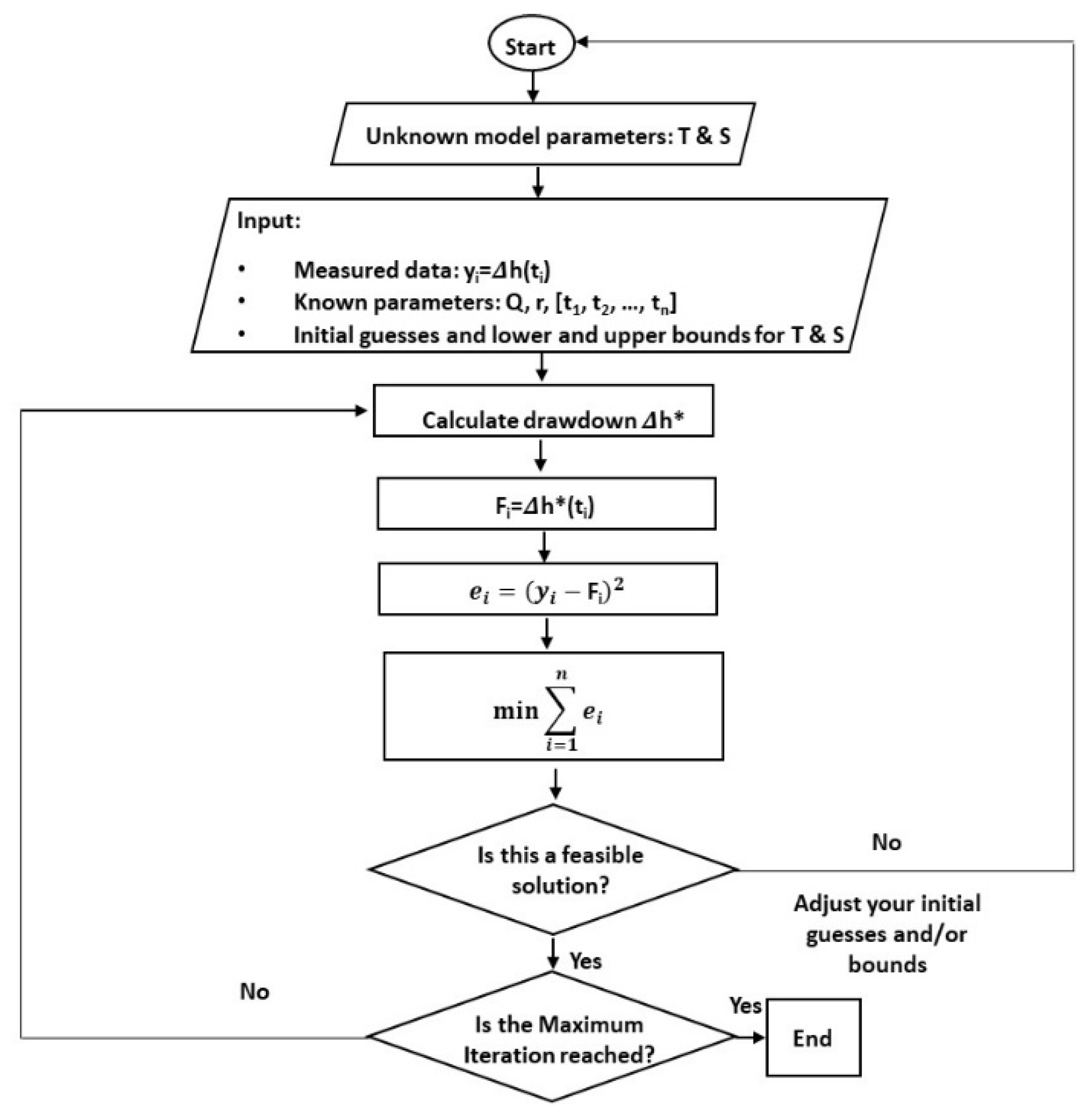
As discussed in the introduction section, the graphic method originally suggested by Theis and later documented by Jacob [12] and others, is often used in textbooks to fit the drawdown data with Equation (1) to estimate the T and S values. The PyTheis script developed in this study employs a nonlinear solver available in the Python curve-fitting library to obtain the best estimates for T and S. The computational steps used by the fitting procedure are summarized in Figure 1.
The scipy.optimize.curve_fit function available in the Python library offers three possible nonlinear solvers: the Levenberg–Marquardt (LM), Trust-Region Reflective (TR), and Dog Box (DB) methods. The LM method is a default algorithm for solving nonlinear least-squares problems using this Python function. LM is an unconstrained nonlinear search procedure typically used for solving small-to-medium-sized problems. This method may fail or converge to a local minimum when inappropriate initial estimates are adopted [26]. TR or DB methods, which are constrained nonlinear search algorithms, are better alternatives when using a limited number of data points to fit nonlinear functions. More recently, Memari and Clement [27] applied all three approaches to fit soil moisture data to various soil water retention models and concluded that the TR is the most robust approach for fitting highly nonlinear functions.
2.3. Initial Guess Values and Parameter Bounds for T and S Values
To use the TR method, one needs to provide parameter bounds and initial guess values. In PyTheis, the initial guess value for T was always set to 1 m2/d. This is a reasonable initial guess since pump tests are usually completed in permeable formations that can produce water. Therefore, assuming that, on average, the aquifer will contain an approximately 1 to 10 m thick layer of fine/silty sand layer with a conductivity of approximately 1 to 0.1 m/day is a good approximation. The lower bound of the T value was assumed to be about 0.01 m2/day, and the upper bound was assumed to be 1.0 × 10⁵. This is a broad range that should cover a wide range of soils. Halford and Kuniansky [18] study summarized hydraulic conductivity values that are typically observed under field conditions. The bounds we have recommended here include all possible T values for permeable sand/silt formations reported in this study.
The minimum value of S was set to 1.0 × 10⁻⁶, which is a typical lower limit of the confined aquifer compressibility value [11]. The maximum value was set to 0.1, which is a typical upper limit for the unconfined specific yield value. The best initial guess value of S was assumed to be 1.0 × 10⁻⁵, which is the typical value of S observed for confined aquifers [11]. These initial guess values and the lower and upper bounds worked well for solving all the example problems considered in this study. However, if needed, users can always modify these default values.
2.4. Estimation of the Error Associated with Transmissivity and Storage Values
Error is an inherent part of every engineering/scientific measurement. One of the major limitations of the Theis graphical method is that the method cannot quantify the error in the estimated values of T and S. Without an error estimate, it is difficult to understand the accuracy of the parameter values, and hence, in most cases, analysts often report the values of T and S using an inappropriate number of significant figures. The Python curve fitting routines employed in this study provides a covariance matrix for the best-fit parameter values. The error associated with the parameter values can be estimated as the square root of the diagonal terms of this covariance matrix. Using this error estimate, the best-fit parameter values can be reported with an appropriate number of significant figures by employing a standard rounding procedure summarized below.
A simple method to determine the number of appropriate significant figures is to express the best-fit parameter values and the associated error values in the scientific notation using a consistent unit. Since the error is an estimate of what we do not know, as a rule of thumb, one should round error estimates to one (max of two, in rare cases) significant figure [28]. Then, one can use the first nonzero digit of the error value to truncate the significant digit of the estimated parameter value [28,29]. For example, if the computer reported a T value of 82.7224131 m2/day and the uncertainty is 3.124124, first express these data in the scientific notation as: T = (8.27224131 ± 0.3124124) × 101 m2/day. After appropriate rounding, the value should then be expressed as: T = (8.3 ± 0.3) × 101 or 83 ± 3 m2/day. The knowledge of the error (or uncertainty) would allow one to round the estimated parameter values using an appropriate number of significant figures. Although this is a well-known standard procedure, when the error estimate is not available analysts often report the estimated values of model parameters with an unrealistic number of significant figures (e.g., see Bateni [24]). We will discuss the implications of this rounding procedure using the results of some benchmark problems in our results section.
3. Test Problems Considered in This Study
To demonstrate the use of PyTheis, we first solve a standard problem given in Lohman [30] to demonstrate the importance of the error estimates and the use of proper rounding to report the parameter values with an appropriate number of significant figures. The dataset given by Lohman [30] describes the drawdown patterns in a theoretical confined aquifer. The monitoring wells are placed at distances of 200, 400, and 800 ft from a well pumping at the constant rate of 96,000 ft3/day. We use these monitoring data to test the performance of the PyTheis code.
We later solve eight other test problems to demonstrate the use of the PyTheis code for solving a variety of previously studied problems with a wide range of model parameters. These eight test problems allowed us to verify whether the default initial guess values and the parameter bounds set within PyTheis can be used to solve practical problems. Finally, we developed three synthetic datasets by artificially introducing different levels of random error into the well-known Walton [31] problem. These perturbed datasets are used to further test the robustness of the fitting procedure when there are considerable random variations in the field data.
4. Results and Discussion
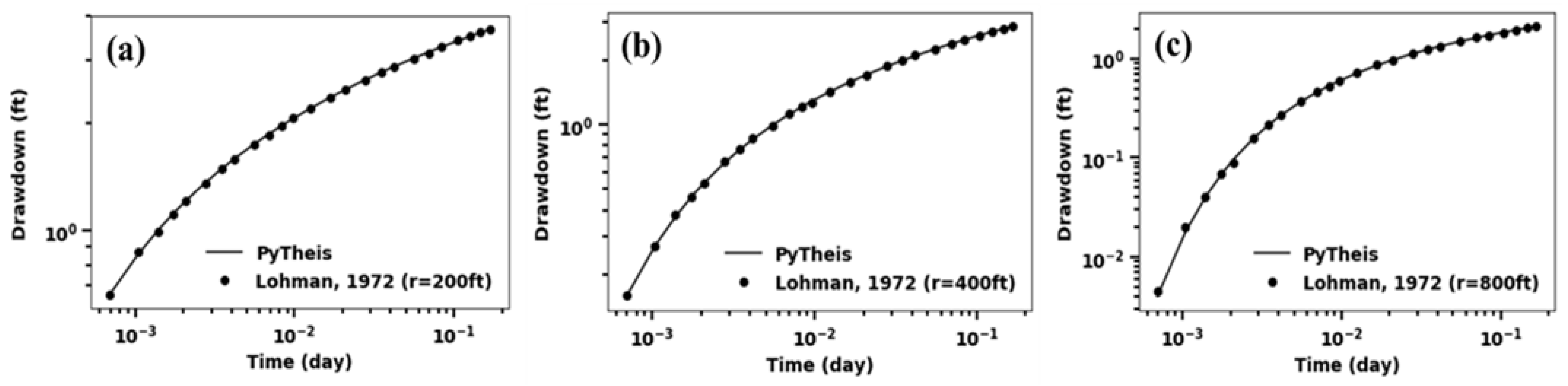
The fitted results estimated using PyTheis for the Lohman [30] test problem are shown in Figure 2. The figures show the fittings for the observed drawdown data collected at three different observation wells located at r = 200, 400, and 800 ft away from the pumping well. The drawdown curves estimated by PyTheis closely fitted the data points (see Figure 2). The best-fit T and S values are close to the values reported in Lohman [30]. For example, the PyTheis estimated model parameters based on data from r = 200 ft are: Tr=200 = 13,379.2554 ft2/day and Sr=200 = 2.01716330 × 10⁻⁴, and the corresponding error values are: 27.3641357 ft2/day and 1.42597139 × 10⁻⁶, respectively. As expected, the computer code reported the best-fit values and error estimates with a large number of significant figures. After appropriate rounding (see the example in Section 2.4), the estimated value of T should be reported as (133.8 ± 0.3) × 102 or 13,380 ± 30 ft2/day. This value compares well with the graphical solution reported in Lohman’s book, which is T = 14,000 ft2/day (note Lohman estimated this average value using the data points from all three wells). In this effort, we evaluated three estimates using the drawdown data reported for the three monitoring wells. The parameter values estimated based on the three datasets are summarized in Table 1. It is worth noting that Lohman’s analysis excluded some extreme data points; for example, when the r2/t values are 108 or more the points fell outside the range of the standard 2 × 4 graph paper and hence were excluded in the analysis. In this study, the PyTheis code was able to utilize all the data points for estimating the model parameters. The results show the model parameter values estimated using all three datasets were close to the average values reported by Lohman. Interestingly, the error analysis shows that the PyTheis estimates are more precise than the value reported by Lohman.
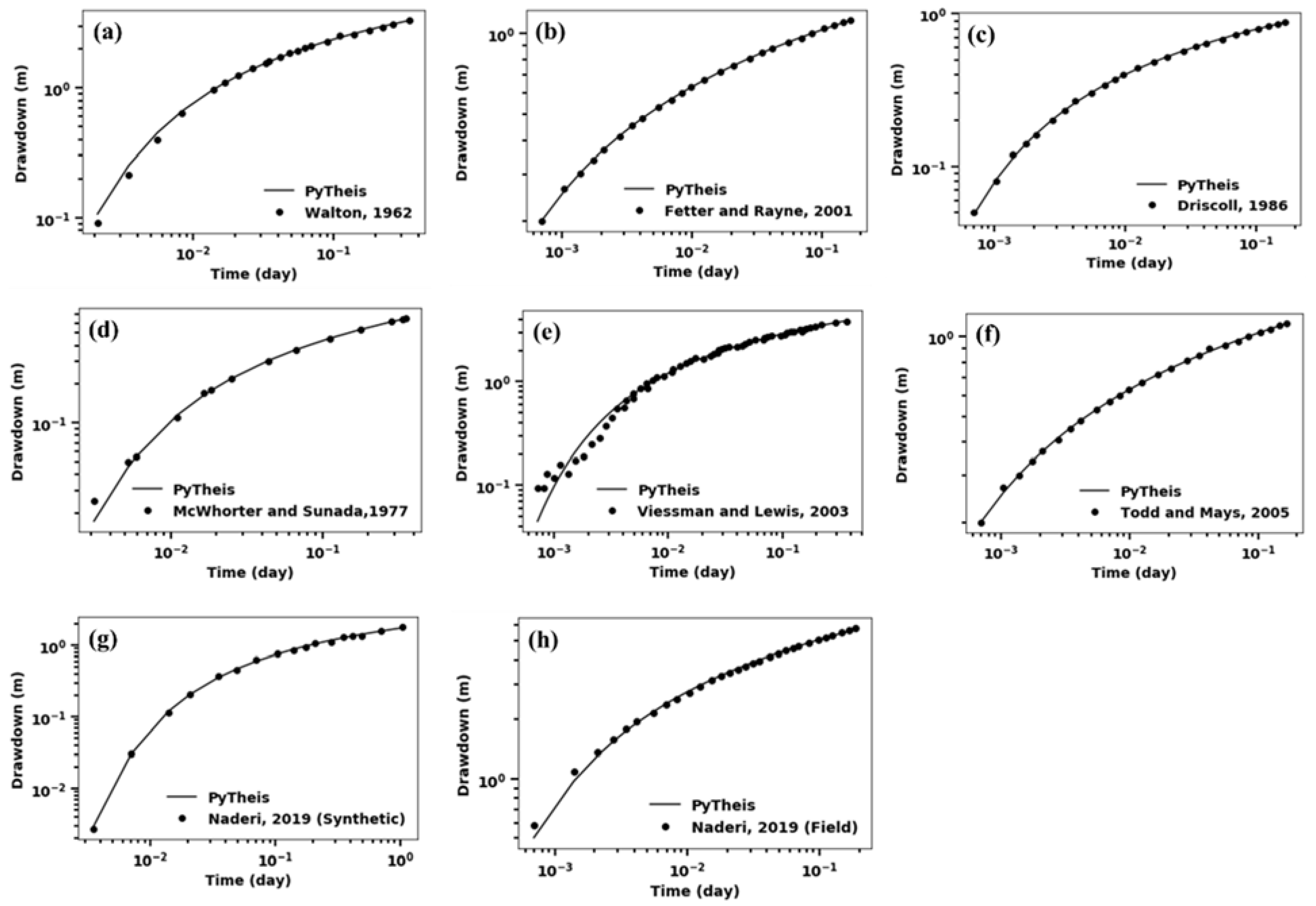
To further test the performance of the PyTheis code under different types of flow conditions, we solved the following eight different problems reported in the literature: Walton [31], Fetter and Rayne [32], Driscol [33], McWhorter and Sunda [34], Viessman and Lewis [35], Todd and Mays [36], and two sets of data from Naderi [23]. Our results indicated that the PyTheis code, with the default initial values and parameter bounds, was able to solve all eight problems. The results for the first problem, the Walton problem, are given in Figure 3a. This problem was based on a pump test completed at a confined aquifer in Gridley, Illinois. This dataset was also used by Saleem [21] for comparing the performance of a least-squares fitting method. The result for the second problem is given in Figure 3b; this problem was taken from Fetter [11] textbook, and the solution was documented in the textbook’s solution manual [32]. The result for the third test problem is shown in Figure 3c; this problem is based on a synthetic test problem given in Driscol [33]. The result for the fourth problem, shown in Figure 3d, is a test problem discussed in McWhorter and Sunda [34]. This dataset is based on a pump test conducted at a field site in Fort Collins, Colorado. The fifth problem, shown in Figure 3e, is an example problem taken from Viessman and Lewis [35]. The sixth problem is taken from Todd and Mays [36] textbook, and the results are shown in Figure 3f; this is a well-known problem that has been widely used in the published literature [22,23] to validate different fitting methods used for estimating aquifer parameter values.
Finally, we selected two different datasets reported in Naderi [23] for our seventh and eighth test problems, and the results are summarized in Figure 3g,h, respectively. Figure 3g results are for a synthetic dataset given in Naderi [23], whereas Figure 3h results are based on a pump test dataset collected at a field site in Shiraz, Iran, and hence, we refer to this dataset as “field data from Naderi (2019)”.
Detailed datas for all eight problems, which include pumping rate, distance from the well, the PyTheis estimated parameter and error values, and the parameter values reported in the literature, are given in Table 2. Since the nonlinear estimation method employed by PyTheis uses a solver that calculates the local optimum, we used these multiple datasets to verify whether the default initial values and parameter bounds are appropriate for estimating realistic aquifer parameter values. The results show that PyTheis converged to values that are close to the literature values reported for these eight test problems.
5. Sensitivity of Parameter Values to Variations in Field Data
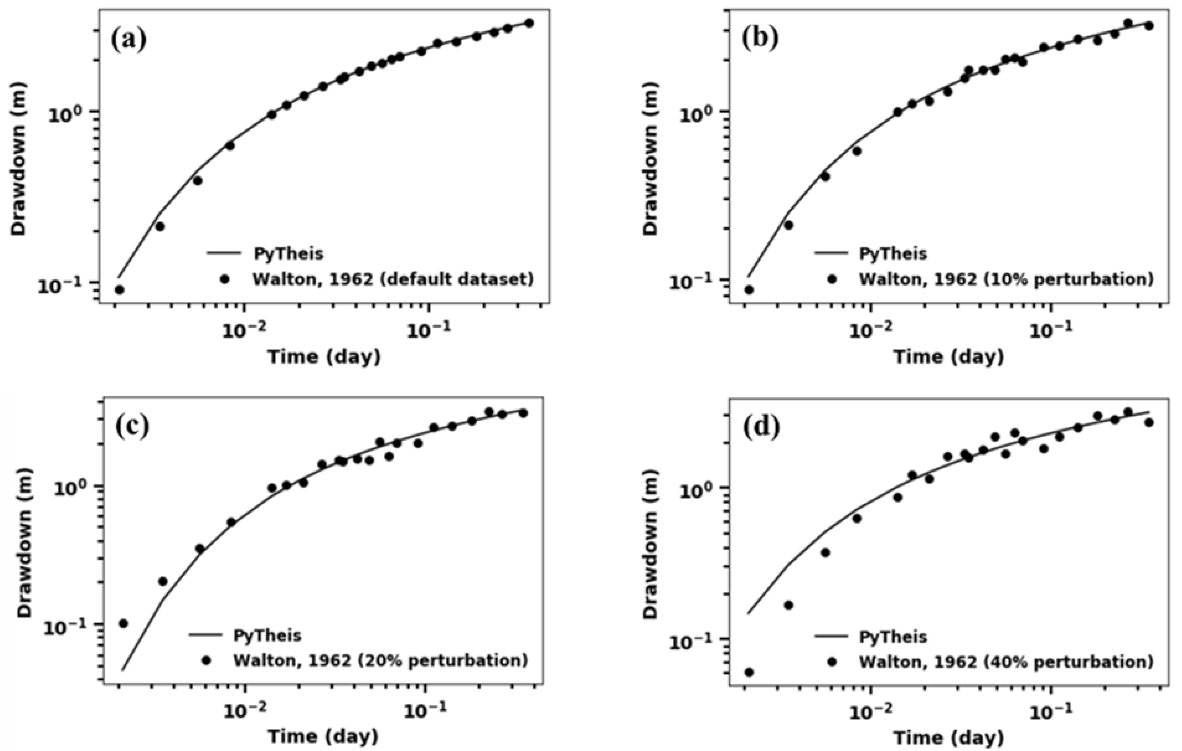
To further test the robustness of the code for solving field problems involving noisy data, we created three synthetic datasets by introducing different levels of random error to the Walton [31] dataset. We used the RANDBETWEEN function in Excel to generate random numbers between the specified range; (−10, 10), (−20, 20), (−40, 40). The field data was perturbed by multiplying these random numbers by the drawdown values and dividing them by 100. The original data along with the three perturbed datasets are given in Appendix B. The PyTheis code was used to fit all four datasets, and the results are shown in Figure 4. As shown in Figure 4a,b, the datasets with a low level of perturbation are located close to the curve estimated by PyTheis over the entire observation period, whereas the datasets with a high level of perturbation (see Figure 4c,d) are scattered farther away from the fitted curve. The best-fit T and S values and the associated errors for all four datasets are summarized in Table 3. The results presented in Table 3 show that the uncertainty in the estimated parameter values increases with an increase in the amount of random error introduced in the dataset. The estimated mean T value for the base case is 123 m2/day and the uncertainty is 1 m2/day. When 10% noise was included in the dataset, the estimated mean value of T is 122 m2/day, and the uncertainty is 4 m2/day. The estimated mean value of S for the base case is 2.1 × 10⁻⁵, and the uncertainty is 4 × 10⁻⁷; and for the 10% perturbed case, the mean S value is 2.1 × 10⁻⁵, and the uncertainty is 1 × 10⁻⁶. It is interesting to note that even for the highly noisy dataset, the predicted mean parameter values are fairly close to the expected values.
6. Conclusions
We present the details of a Python tool, namely, PyTheis, for evaluating the aquifer properties T and S, and the error associated with these two important hydrogeological parameters. PyTheis is an excellent alternative to the commonly used graphical estimation method (known as the Theis type-curve method), which involves laborious curve matching steps that can result in subjective estimates. The method proposed in this study can be used within the public domain Python platform, and it is a rational, modern alternative to the traditional, 90-year-old Theis graphical procedure. PyTheis is a flexible computer code that uses open-source tools. The initial guess values and parameter bounds suggested in this study worked well for fitting a wide variety of pump test data. PyTheis is a practical tool for analyzing pump tests, and it is also an excellent teaching tool. Furthermore, this code can be easily adapted to solve other hydrological parameter estimation problems that require nonlinear curve fitting routines.
It is important to note that the current version of PyTheis uses the basic confined flow analytical solution. Therefore, the users must carefully screen the field data to avoid forcing the ideal Theis curve to fit the data points that are inconsistent with the theory. For example, in many cases, early time data points collected during a pump test are strongly influenced by well storage effects. Similarly, river/rock boundary conditions and leaky confining layers will impact the later time data points. Forced fitting the Theis model to these early or later data points will yield incorrect aquifer parameter values. Therefore, the users should use caution and carefully screen the field data before using the code to fit the classic Theis model. Correcting the code for well-storage, boundary-condition, and leaky-aquifer effects is beyond the scope of this study. Future studies should consider including advanced analytical or numerical models that can account for these effects.
Author Contributions
Conceptualization, S.W.C. and T.P.C.; methodology, S.W.C. and T.P.C.; software, S.W.C. and S.S.M.; validation, S.W.C., S.S.M. and T.P.C.; formal analysis, S.W.C., S.S.M. and T.P.C.; investigation, S.W.C. and T.P.C.; resources, S.W.C. and T.P.C.; data curation, S.W.C. and S.S.M.; writing—original draft preparation, S.W.C. and S.S.M.; writing—review and editing, S.W.C., S.S.M. and T.P.C.; visualization, S.W.C. and S.S.M.; supervision, T.P.C.; project administration, T.P.C.; funding acquisition, S.W.C. and T.P.C. All authors have read and agreed to the published version of the manuscript.
Funding
This research was, in part, supported by a National Science Foundation (Grant Award No. 2019561) and by a grant from the Development Program of Minimizing of Climate Change Impact Technology funded through the National Research Foundation of Korea (NRF) of the Korean government (Grant No. NRF-2020M3H5A1080735).
Institutional Review Board Statement
Not applicable.
Informed Consent Statement
Not applicable.
Data Availability Statement
The code is given in the Appendix A, and all required data are provided within the text.
Acknowledgments
We like to thank Water reviewers for provided several useful suggestions.
Conflicts of Interest
The authors declare no conflict of interest.
Appendix A
PyTheis Code
Input instructions: prepare an excel file entering all non-zero times (do not include the zero) in column A and drawdown in column B. Save the file as a “csv” file (theisdata.csv) in the local directory where PyTheis is saved.
import numpy as np
import math as m
import matplotlib.pyplot as plt
from scipy.optimize import curve_fit
def wufunc(r,S,T,t):
u = (r**2)*S/(4*T*t)
Wu=-0.5772-np.log(u)+u
ntrm = 30
for i in range (2, ntrm+1):
sign = (-1)**(i-1)
factval = float(m.factorial(i))
Wu = Wu + sign*(u**i)/(i*factval)
#End loop i
return (Wu)
def myfunc(tt, T, S):
pi = 3.14
Q = 1199.22 #m3/d
r = 251.155 #m
nrow = len(tt)
n= nrow
drawdown=np.zeros((n),float)
for i in range (0,n):
Wu_val=wufunc(r,S,T,tt[i])
drawdown[i] = Q*Wu_val/(4*pi*T)
#End loop i
return (drawdown)
def main():
indata = np.loadtxt("theisdata.csv", delimiter=",")
Times = np.copy(indata[:,0]) # Time from first column
sobs = np.copy(indata[:,1]) # Drawdown from second column
init_vals = [1, 0.00001] # for [T & S values]
best_vals, covar = curve_fit(myfunc, Times, sobs, p0=init_vals, bounds=([0.01, 0.000001], [100000, 0.1]), method = ‘trf’)
stdevs = np.sqrt(np.diag(covar))
plt.xscale(‘log’)
plt.yscale(‘log’)
print (‘Best valus (T, S)’)
print (best_vals)
print (‘Covariance’)
print (covar)
print (‘standard deviation’)
print (stdevs)
T = best_vals [0]
S = best_vals [1]
smodel=myfunc(Times,T,S)
plt.plot(Times,smodel)
plt.plot(Times, sobs, ‘bo’)
plt.xlabel("Time (day)")
plt.ylabel("Drawdown (m)")
plt.show()
main()
Appendix B

Table A1.
Time (day) vs. drawdown (m) data for the perturbed Walton (1962) problem.
| Time (Day) | Drawdown (Base Case) | Drawdown (±10%) | Drawdown (±20%) | Drawdown (±40%) |
|---|---|---|---|---|
| 0.002083 | 0.09144 | 0.087782 | 0.102413 | 0.061265 |
| 0.003472 | 0.21336 | 0.21336 | 0.206959 | 0.170688 |
| 0.005556 | 0.39624 | 0.41209 | 0.356616 | 0.38039 |
| 0.008333 | 0.64008 | 0.588874 | 0.544068 | 0.64008 |
| 0.013889 | 0.97536 | 0.994867 | 0.965606 | 0.877824 |
| 0.016667 | 1.09728 | 1.119226 | 1.02047 | 1.217981 |
| 0.020833 | 1.24968 | 1.162202 | 1.062228 | 1.149706 |
| 0.026389 | 1.43256 | 1.317955 | 1.446886 | 1.618793 |
| 0.032639 | 1.55448 | 1.58557 | 1.52339 | 1.678838 |
| 0.034722 | 1.61544 | 1.776984 | 1.502359 | 1.599286 |
| 0.041667 | 1.73736 | 1.772107 | 1.563624 | 1.789481 |
| 0.048611 | 1.85928 | 1.766316 | 1.543202 | 2.175358 |
| 0.055556 | 1.92024 | 2.035454 | 2.093062 | 1.709014 |
| 0.0625 | 2.04216 | 2.083003 | 1.633728 | 2.348484 |
| 0.069444 | 2.1336 | 1.984248 | 2.02692 | 2.048256 |
| 0.090278 | 2.286 | 2.4003 | 2.01168 | 1.85166 |
| 0.111111 | 2.52984 | 2.479243 | 2.656332 | 2.200961 |
| 0.138889 | 2.5908 | 2.72034 | 2.694432 | 2.538984 |
| 0.180556 | 2.80416 | 2.663952 | 2.97241 | 3.000451 |
| 0.222222 | 2.95656 | 2.897429 | 3.400044 | 2.838298 |
| 0.263889 | 3.10896 | 3.357677 | 3.295498 | 3.202229 |
| 0.347222 | 3.32232 | 3.22265 | 3.388766 | 2.724302 |
References
- Cooper, H.H.; Jacob, C.E. A generalized graphical method for evaluating formation constants and summarizing well-field history. Eos Trans. Am. Geophys. Union 1946, 27, 526–534. [Google Scholar] [CrossRef]
- Hantush, M.S. Analysis of data from pumping tests in leaky aquifers. Eos Trans. Am. Geophys. Union 1956, 37, 702–714. [Google Scholar] [CrossRef]
- Kruseman, G.P.; de Ridder, N.A. Analysis and Evaluation of Pumping Test Data; International Institute for Land Reclamation and Improvement: Wageningen, The Netherlands, 1994. [Google Scholar]
- Neuman, S.P. Theory of flow in unconfined aquifers considering delayed response of the water table. Water Resour. Res. 1972, 8, 1031–1045. [Google Scholar] [CrossRef]
- Theis, C.V. The relation between the lowering of the piezometric surface and the rate and duration of discharge of a well using ground water storage: Transaction of American Geophysical Union. Trans. Am. Geophys. Union 1935, 16, 519–524. [Google Scholar] [CrossRef]
- Walton, W.C. Comprehensive Analysis of Water-Table Aquifer Test Data. Groundwater 1978, 16, 311–317. [Google Scholar] [CrossRef]
- Benbarka, A.M.; Davis, D.R. Aspects of Aquifer Test Error Analysis; Arizona-Nevada Academy of Science: Glendale, AZ, USA, 1981. [Google Scholar]
- Naderi, M.; Gupta, H.V. On the Reliability of Variable-Rate Pumping Test Results: Sensitivity to Information Content of the Recorded Data. Water Resour. Res. 2020, 56, e2019WR026961. [Google Scholar] [CrossRef]
- Khan, I.A. Determination of Aquifer Parameters Using Regression Analysis1. JAWRA J. Am. Water Resour. Assoc. 1982, 18, 325–330. [Google Scholar] [CrossRef]
- McElwee, C.D. Theis Parameter Evaluation from Pumping Tests by Sensitivity Analysis. Groundwater 1980, 18, 56–60. [Google Scholar] [CrossRef]
- Fetter, C.W. Applied Hydrogeology; Prentice Hall: Upper Saddle River, NJ, USA, 2001. [Google Scholar]
- Jacob, C.E. On the flow of water in an elastic artesian aquifer. Eos Trans. Am. Geophys. Union 1940, 21, 574–586. [Google Scholar] [CrossRef]
- Wenzel, L.K.; Fishel, V.C. Methods for Determining Permeability of Water-Bearing Materials with Special Reference to Discharging Well Methods, Water-Supply Paper 887; United States Government Printing Office: Washington, DC, USA, 1942.
- Labadie, J.W.; Helweg, O.J. Step-drawdown test analysis by computer. Groundwater 1975, 13, 438–444. [Google Scholar] [CrossRef]
- Reed, J.E. Type Curves for Selected Problems of Flow to Wells in Confined Aquifers; 03-B3; U.S. Geological Survey: Washington, DC, USA, 1980.
- Maslia, M.L.; Randolph, R.B. Methods and Computer Program Documentation for Determining Anisotropic Transmissivity Tensor Components of Two-Dimensional Ground-Water Flow; 86-227; U.S.Geological Survey: Reston, VA, USA, 1986.
- Barlow, P.M.; Moench, A.F. WTAQ: A Computer Program for Calculating Drawdowns and Estimating Hydraulic Properties for Confined and Water-Table Aquifers; 99-4225; U.S. Geological Survey: Northborough, MA, USA, 1999.
- Halford, K.J.; Kuniansky, E.L. Documentation of Spreadsheets for the Analysis of Aquifer-Test and Slug-Test Data; 2002-197; U.S. Geological Survey: Carson City, NV, USA, 2002.
- Duffield, G.M. AQTESOLV for Windows Version 4.5 User’s Guide; HydroSOLVE Inc.: Reston, VA, USA, 2002. [Google Scholar]
- WaterlooHydrogeologic. Aquifer Test Pro. Users Manual. Graphical Analysis and Reporting of Pumping Test and Slug Test Data; WaterlooHydrogeologic: Waterloo, ON, Canada, 2002; p. 267. [Google Scholar]
- Saleem, Z. A computer method for pumping-test analysis. Groundwater 1970, 8, 21–24. [Google Scholar] [CrossRef]
- Yeh, H.D. Theis’ Solution by Nonlinear Least-Squares and Finite-Difference Newton’s Method. Groundwater 1987, 25, 710–715. [Google Scholar] [CrossRef]
- Naderi, M. Estimating confined aquifer parameters using a simple derivative-based method. Heliyon 2019, 5, e02657. [Google Scholar] [CrossRef] [PubMed] [Green Version]
- Bateni, S.M.; Mortazavi-Naeini, M.; Ataie-Ashtiani, B.; Jeng, D.S.; Khanbilvardi, R. Evaluation of methods for estimating aquifer hydraulic parameters. Appl. Soft Comput. J. 2015, 28, 541–549. [Google Scholar] [CrossRef]
- Fletcher, R. Practical Method of Optimization: Unconstrained Optimization; John Wiley & Sons: Hoboken, NJ, USA, 1980; Volume 1. [Google Scholar]
- Aster, R.C.; Borchers, B.; Thurber, C.H. Parameter Estimation and Inverse Problems; Elsevier: Amsterdam, The Netherlands, 2005. [Google Scholar]
- Memari, S.S.; Clement, T.P. PySWR—A Python Code for Fitting Soil Water Retention Functions. Comput. Geosci. 2021, 156, 104897. [Google Scholar] [CrossRef]
- Harria, D.H. Quantitative Chemical Analysis; W. H. Freeman: New York, NY, USA, 2007. [Google Scholar]
- Taylor, J.R. An Introduction to Error Analysis, 2nd ed.; University Science Books: New York, NY, USA, 1997. [Google Scholar]
- Lohman, S.W. Ground-Water Hydraulics; 708; U.S. Geological Survey: Washington, DC, USA, 1972.
- Walton, W.C. Selected Analytical Methods for Well and Aquifer Evaluation; Illinois State Water Survey: Urbana, IL, USA, 1962. [Google Scholar]
- Fetter, C.W.; Rayne, T. Applied Hydrology Solutions Manual, 4th ed.; Prentice Hall: Upper Saddle River, NJ, USA, 2001. [Google Scholar]
- Driscol, F.G. Groundwater and Wells, 2nd ed.; Johnson Division: St Paul, MN, USA, 1986. [Google Scholar]
- McWhorter, D.B.; Sunada, D.K. Ground Water Hydrology and Hydraulics; Water Resources Publications, LLC: Fort Collins, CO, USA, 1977; p. 290. [Google Scholar]
- Viessman, W.; Lewis, G.L. Introduction to Hydrology, 5th ed.; Pearson Eduction, Inc.: Upper Saddle River, NJ, USA, 2003. [Google Scholar]
- Todd, D.K.; Mays, L.W. Groundwater Hydrology; John Wiley & Sons, Inc.: New York, NY, USA, 2005. [Google Scholar]
Figure 1.
Flowchart describing for fitting procedure.

Figure 2.
Log–log scale time-drawdown curves fitted using the PyTheis code for the Lohman (1972) datasets: (a) 200 ft data, (b) 400 ft data, and (c) 800 ft data.
Figure 2.
Log–log scale time-drawdown curves fitted using the PyTheis code for the Lohman (1972) datasets: (a) 200 ft data, (b) 400 ft data, and (c) 800 ft data.

Figure 3.
Log–log scale time-drawdown curves fitted using the PyTheis code for the literature problems: (a) Walton (1962), (b) Fetter and Rayne (2001), (c) Driscoll (1986), (d) McWhorter and Sunada (1977), (e) Viessman and Lewis (2003), (f) Todd and Maya (2005), (g) Synthetic data from Naderi (2019), and (h) field data from Naderi (2019). The data points were taken from the tables/figures reported in these publications.

Figure 4.
Log–log scale time-drawdown curves fitted using the PyTheis code for the perturbed Walton (1962) problems: (a) base case data, (b) ±10% perturbation, (c) ±20% perturbation, and (d) ±40% perturbation.
Figure 4.
Log–log scale time-drawdown curves fitted using the PyTheis code for the perturbed Walton (1962) problems: (a) base case data, (b) ±10% perturbation, (c) ±20% perturbation, and (d) ±40% perturbation.

Table 1.
PyTheis estimated transmissivity (T) and storage values (S) for the Lohman (1972) problem.
| Distance from Well (ft) | Lohman (1972) | PyTheis estimated values of T (ft2/day) | |
|---|---|---|---|
| Code Output | Rounded Values | ||
| 200 | 14,000 | 13,379.2554 ± 27.3641357 | 13,380 ± 30 |
| 400 | 13,405.8670 ± 43.1205549 | 13,410 ± 40 | |
| 800 | 13,339.4913 ± 49.1948724 | 13,340 ± 50 | |
| Distance from Well (ft) | Lohman (1972) | PyTheis estimated value of S (dimensionless) | |
| Code Output | Rounded Values | ||
| 200 | 2 × 10⁻⁴ | 2.01716330 × 10⁻⁴ ± 1.42597139 × 10⁻⁶ | (2.02 ± 0.01) × 10−4 |
| 400 | 2.0120642 × 10⁻⁴ ± 1.60789185 × 10⁻⁶ | (2.01 ± 0.02) × 10−4 | |
| 800 | 2.02306304 × 10⁻⁴ ± 1.24751164 × 10⁻⁶ | (2.01 ± 0.01) × 10−4 | |
Table 2.
Details of the eight test problems used in this study. The table also provides the T and S values estimated by PyTheis along with literature data.
Table 2.
Details of the eight test problems used in this study. The table also provides the T and S values estimated by PyTheis along with literature data.
| Reference | Input | Output | |||
|---|---|---|---|---|---|
| Input Variable | Values | Parameter | Literature Data | PyTheis | |
| Walton (1962) | Q (m3/day) R (m) | 1199.52 251.25 | T (m2/day) S | 125.4 2.0 × 10⁻⁵ | 123 ± 1 (2.10 ± 0.04) × 10−5 |
| Fetter and Rayne (2001) | Q (m3/day) R (m) | 1090.2 76.2 | T (m2/day)S | 498 5.17 × 10⁻⁵ | 498 ± 1 (5.18 ± 0.04) × 10−5 |
| Driscoll (1986) | Q (m3/day) R (m) | 2730 122 | T (m2/day) S | 1250 1.9 × 10⁻⁴ | 1249± 5 (2.01 ± 0.02) × 10−4 |
| McWhorter and Sunada (1977) | Q (m3/day) R (m) | 2695.68 20 | T (m2/day) S | 1175 5.3 × 10⁻² | 1250 ± 10 (5.8 ± 0.1) × 10−2 |
| Viessman and Lewis (2003) | Q (m3/day) R (m) | 5450.99 91.44 | T (m2/day) S | 601.45 3 × 10⁻⁴ | 562 ± 5 (3.62 ± 0.08) × 10−4 |
| Todd and Mays (2005) | Q (m3/day) R (m) | 2500 60 | T (m2/day) S | 1110 2.06 × 10⁻⁴ | 1139 ± 5 (1.93 ± 0.03) × 10−4 |
| Naderi (2019) (Synthetic) | Q (m3/day) R (m) | 14,400 50 | T (m2/day) S | 2517 0.05 | 2520 ± 60 (5.0 ± 0.2) × 10−2 |
| Naderi (2019) (Field) | Q (m3/day) R (m) | 3888 51 | T (m2/day) S | 305 1.8×10⁻⁴ | 306 ± 2 (1.81 ± 0.04) × 10−4 |
Table 3.
PyTheis estimated T and S values for the perturbed Walton (1962) datasets.
| Case | PyTheis estimated values of T (m2/day) | |
|---|---|---|
| Code Output | Rounded Values | |
| Base Walton (1962) | 123.151860 ± 1.20663423 | 123 ± 1 |
| ±10% perturbation | 121.984308 ± 4.21487923 | 122 ± 4 |
| ±20% perturbation | 106.109730 ± 5.70221135 | 106 ± 6 |
| ±40% perturbation | 136.534842 ± 10.4565877 | 140 ± 10 |
| Case | PyTheis estimated values of S (dimensionless) | |
| Code Output | Rounded Values | |
| Base Walton (1962) | 2.09488656 × 10⁻⁵ ± 4.02955356 × 10⁻⁷ | (2.10 ± 0.04) × 10−5 |
| ±10% perturbation | 2.11467086 ×10⁻⁵ ± 1.42507828 × 10⁻⁶ | (2.1 ± 0.1) × 10−5 |
| ±20% perturbation | 2.73691488 × 10⁻⁵ ± 2.48293150 × 10⁻⁶ | (2.7 ± 0.2) × 10−5 |
| ±40% perturbation | 1.83710673 × 10⁻⁵ ± 2.98924137 × 10⁻⁶ | (1.8 ± 0.3) × 10−5 |
Publisher’s Note: MDPI stays neutral with regard to jurisdictional claims in published maps and institutional affiliations. |
© 2021 by the authors. Licensee MDPI, Basel, Switzerland. This article is an open access article distributed under the terms and conditions of the Creative Commons Attribution (CC BY) license (https://creativecommons.org/licenses/by/4.0/).
Share and Cite
MDPI and ACS Style
Chang, S.W.; Memari, S.S.; Clement, T.P. PyTheis—A Python Tool for Analyzing Pump Test Data. Water 2021, 13, 2180. https://doi.org/10.3390/w13162180
AMA Style
Chang SW, Memari SS, Clement TP. PyTheis—A Python Tool for Analyzing Pump Test Data. Water. 2021; 13(16):2180. https://doi.org/10.3390/w13162180
Chicago/Turabian StyleChang, Sun Woo, Sama S. Memari, and T. Prabhakar Clement. 2021. "PyTheis—A Python Tool for Analyzing Pump Test Data" Water 13, no. 16: 2180. https://doi.org/10.3390/w13162180
Note that from the first issue of 2016, this journal uses article numbers instead of page numbers. See further details here.