
Time Evolution Study of the Electric Field Distribution and Charge Density Due to Ion Movement in Salty Water


1
Department of Food Science and Technology, Faculty of Food Science, Campus Alsos Egaleo, University of West Attica, Ag. Spyridonos 28, 12243 Athens, Greece
2
Department of Mechanical Engineering, University of West Attica, 12244 Athens, Greece
*
Author to whom correspondence should be addressed.
Water 2021, 13(16), 2185; https://doi.org/10.3390/w13162185
Submission received: 15 July 2021
/
Revised: 6 August 2021
/
Accepted: 8 August 2021
/
Published: 10 August 2021
(This article belongs to the Special Issue Sustainable Processes for the Removing of Heavy Metals from Aqueous Solutions)
Abstract
:Desalination and water purification through the ion drift of salted water flow due to an electric field in a duct is perhaps a feasible membrane-free technology. Here, the unsteady modulation of ion drift is treated by employing the Poison–Nernst–Plank (PNP) equations in the linear regime. Based on the solution of the PNP equations, the closed-form relationships of the charge density, the ion concentration, the electric field distribution and its potential are obtained as a function of position and time. It is found that the duration of the ion drift is of the order of one second or less. Moreover, the credibility of various electrical circuit models is examined and successfully compared with our solution. Then, the closed form of the surface charge density and the potential that are calculated without the linear approximation showed that the compact layer is crucial for the ion confinement near the duct walls. To test this, nonlinear solutions of the PNP equations are obtained, and the limits of accuracy of the linear theory is discussed. Our results indicate that the linear approximation gives accurate results only at the fluid’s bulk but not inside the double layer. Finally, the important issue of electric field diminishing at the fluid’s bulk is discussed, and a potential method to overcome this is proposed.
1. Introduction
Research on desalination and ion removal methods from a water solution, in general, is of crucial importance for freshwater sustainability. Except for the classical methods, such as the multi-stage flash distillation (MSF), multiple effect distillation and vapor compression distillation [1,2,3,4,5,6,7,8,9,10,11], other methods based on special membranes or electrodes, such as the electrodialysis and the reverse osmosis (RO) electro-deionization, electrophoresis, electroosmosis and capacitive deionization [12,13,14,15,16,17,18,19,20,21,22,23,24,25,26,27,28,29,30,31,32,33,34,35,36], have recently been developed. The bottleneck of all the above methods, which are based on the ion drift due to electric fields, is the attempt to resolve the formation of a double layer, i.e., a boundary layer adjacent to the electrodes. Upon its formation, due to ion confinement at the higher potential region of the electrodes, no electric force remains to attract other ions from the fluid’s bulk.
Recently, we proposed the electric ion drift (EID) method, which works similarly to the capacitive deionization method but without the use of membranes or special electrodes [37]. Our method is based on the ion drift due to the application of an electric field from a capacitor externally placed from the solution. A similar configuration to the EID method is studied by molecular dynamics simulations and proved that the proposed method can successively drift salt ions in nanochannels [27]. This method works similarly to the capacitive deionization method [38,39,40,41,42,43,44,45], but in its original concept, it is more elegant since no porous electrodes are required. The EID method is of the same energy consumption as the capacitive deionization method of about 0.2 kWh/m3 and can only be efficient in low salt concentrations as it is presented in our following work [46] for solution equilibrium but without the use of membranes or special electrodes. There, the spatial distributions of the electric field and potential, the ion concentration and also the electric charge confined adjacent to the walls are presented for various applied external fields and duct widths.
An in-depth investigation is performed here for the salty water solution flow in a duct that is submerged into an external electric field using the Poisson–Nernst–Planck (PNP) equations and considering the double-layer formation bottleneck. Both the temporal and the spatial distributions are studied. The model equations and details are described in Section 2. By considering the Stern model, the closed-form solutions of charge density, ion concentration, electric field intensity and potential are presented in the linear regime in Section 3. The spatial and temporal distributions found are compared to existing electric circuit models and the equilibrium distributions of Reference [46].
The linear approximation is incapable of providing reasonable results neither for the surface charge density nor for the electric field or potential in the electrodes nearby area (adjacent to the duct walls), i.e., inside the double layer. This analysis is made in Section 4, and a novel method to calculate the surface charge density and the other field quantities is proposed. Lastly, the non-linear PNP equation is deployed in Section 5, and the conditions under which the linear model is valid are investigated. Finally, in Section 6 and Section 7, we proceed to compare our results with any experimental data available and to draw the most important conclusions.
2. Model Equations and Mathematical Evaluation
It is assumed that positive and negative ions of equal concentrations are diluted in a water solution. The salted water flows in a duct, while the duct is subjected to a steady-state and homogeneous electric field created by a pair of plate electrodes, which are under voltage V (Figure 1). The external electric field intensity E has a direction normal to the plate electrodes from positive to negative along the y-axis. The fluid is flowing in the duct perpendicular to the external electric field with velocity . Thus, ions are moving due to the combined motion of the water flow along the streamwise direction and along the y-axis due to the electric force with velocity . The y-axis ionic flux of the positive ions is given by the relation , where is the concentration of the positive ions. From the analysis that is presented in Appendix A and Equation (A5), we have
where z is the number of overflow protons; ; (see Appendix A) is the mobility of the positive ions, with being the dynamic viscosity of water and being the effective radius of the ions; φ is the electric potential in the fluid’s bulk; and is the diffusion coefficient of the positive ion. is the Boltzmann constant; R = 8.314 J/(mol K); is the Avogadro constant; and T is the absolute temperature, which is considered T = 300 K throughout this work.
In the above Equation (1), the electric field is substituted by . Following the same procedure, the ionic flux of the negative ions is read as , where z is the number of overflow electrons. Considering that both positive and negative ions have the same z, the same mobility and, thus, , the ionic fluxes can be read more simply as
where the sign of the ionic fluxes indicates the direction of motion and z is considered positive.
The concentration conservation equation may read as
where the concentration is in (mol/) and the ionic fluxes in .
The charge density due to the above ion concentration reads as
and F = 96,485.34 C/mol is the Faraday constant.
By applying the 1D Poisson equation in the y-direction of the duct, it is found that
The above Equations (3) and (5) constitute the so-called Poisson–Nernst–Planck (PNP) equations system, which is solved in the next Section.
It should be noticed that the present study is in accordance with the Debye–Huckel theory [47,48,49,50], also used in References [37,46], where water is considered as a continuous dielectric medium. Thus, the external electric field effect in water is to initiate change in its electric permittivity in the solution to , where is the relative permittivity of the water and .
3. PNP Equations Solution for the Stern Model
3.1. Boundary Conditions
For the study of the model, the general Stern model can be used where the ions have finite dimensions and thus can only approach to a small distance from the wall of the duct. The contribution of the Stern model is analytically discussed in Appendix B.
Before discussing the solution of the PNP equations, we must define the appropriate boundary conditions. In the center of the duct, at , the electric potential is kept equal to zero, , while and are the potential at y = 0 and , respectively. Thus, by considering a linear relation of distance for the potential at the compact part of the double layer adjacent to the two electrodes, we have
where is the effective thickness of the compact part of the double layer [51,52] (see Appendix B).
Moreover, since the process is a non-Faradaic one [52,53], because no charge is transferred through the electrodes, the ion fluxes and the current density should be zero at the boundaries, i.e.,
Finally, the initial conditions of the model are such that a uniform ion distribution is applied at t < 0, together with a zero potential.
3.2. Linearized Solution of the PNP Equation
We considered that the ion concentration in the fluid’s bulk is supposed to slightly change linearly along the y-direction from 0 to L. As the ion concentrations are linearly increased or decreased to opposite walls, the total concentration is constant; i.e., the total charge density is lower than the density of each ion (either positive or negative) [52,54,55,56]. Thus, most of the solution bulk is quasi-neutral, except in the double layer, i.e., a boundary layer of width of the order of 1 μm or less. Thus, from Equation (3), it is found that
Considering that , where is the concentration of each ion in the center of the duct (equal for the two ions due to symmetry), subtracting the above equations and by recalling that the charge density is given by the relationship:
it is found that
where
Thus, the width corresponds to the so-called Debye length due to the capacitor that may simulate the diffuse layer according to the Gouy–Chapman theory at the edges of the duct. The analytical solution of Equation (12) is given in Appendix C and results in the following relations:
where
and
Thus, from the charge density, it is found that the concentrations of the positive and negative ions are varied as
Validation of the Electric Circuit Models for Long Ducts
In case of a duct of width of mm order or wider, , and since , it is found for the rate and, thus, may be considered almost equal to zero. Moreover, for such length of the duct and since , it can also be considered that . Thus, after these simplifications:
As it may be observed, the quantities in Equations (14)–(21) are exponentially varied, and τ is a characteristic time, the so-called time constant. Here, the above theory fits to the Gouy–Chapman and Stern theories that consider the solution as an RC circuit (see Appendix B), because the characteristic time of the above analysis is exactly the same as the time of the RC circuit (compare Equations (22) and (A10)). Since the fluid bulk is in quasi-neutral condition, its resistance per unit surface is equal to (Equation (A7)), and for the time constant effective capacitor (due to the charge confinement at the edges), we have
As it may be observed, Equation (24) is exactly the same as the Stern’s model (see Appendix B) as would be expected. Thus, we have shown that the electric model in long ducts is equal to the linear PNP equation solution, and it is valid under the same assumptions for the solution. The time duration to the end of the phenomenon is plotted in Figure 2 for the case of ions, for the salted water solution of (), as a function of the initial concentration and various duct widths. As always for the exponentially decay variations, equilibrium is expected after . Thus, here it will also be achieved in less than a second at the most as it is observed in Figure 2.
3.3. Long Time Behavior
As the time increases, then and , and Equations (14)–(21) have their equilibrium forms as
The equilibrium solutions of Equations (25)–(29) can be easily verified by the recent results of Reference [46] for the present water solution with (in S.I. (System International)) (from Equation (19)) and . For , where and thus and for , and by considering the effect as negligible due to the compact layer, i.e., , Equations (25)–(27) are exactly the same as in Reference [46]. However, the concentration Equations (28) and (29) are different than the ones of Reference [46] that read as
The first observation is that Equations (28) and (29) are expected to differ from Equations (30) and (31) of Reference [46] due to the linearization of the exponential term . This happens when , which is the same as the linearization of the exponential function when only the first two terms of the Taylor expansion are kept. Thus, Equations (30) and (31) are more accurate and are used for comparison in the next sections where nonlinear terms are considered for the PNP equation. Moreover, the linear approximation is valid along the duct width, Reference [46], for
which is also applied for the linearized PNP solution. By using Equations (25)–(29) and after some calculus, it can easily be determined that the electric potential and electric field become zero at the fluid bulk, as the width of the duct, the initial concentration and the potential φ(0) are increased as is also discussed in Reference [46]. As it is illustrated below, the linear approximation gives reasonable results at the fluid’s bulk.
Furthermore, the surface charge density (in ) can be found by integrating Equation (25) of the linearized PNP solution as
and its absolute value adjacent to each electrode is given for as
Based on the above approximations, , the surface charge density is found to be exactly the same as the electric circuit RC model as
4. Exact Evaluation of the Electric Field and the Surface Charge Density
The calculation of the electric field and the surface charge density under steady-state conditions is presented below without the linear approximation. Starting from the electric field definition:
and by considering and the electric field intensity is in the center of the duct, and by integrating it, it is found that
where
which is valid only inside the diffuse layer and not in the compact layer, thus, in regions where the Boltzmann distribution is valid. In this region, is almost diminished relative to the values of the second part of the undersquare quantity; thus,
and close to the positive electrode:
The integration of the 1D Poisson equation from to can give the surface charge density near the walls as , where is the surface charge density (in C/m2) near the positive electrode. Applying that , it is , which due to Equation (35) gives
where is the potential at the outer Helmholtz plane (OHP) at distance .
It should be noticed that due to continuity, the electric field magnitude is equal at both sides of the OHP, i.e., of the diffuse layer but also of the compact layer side. Moreover, electric field magnitude is almost constant along the compact layer. Thus, for the positive electrode, it is , and by replacing in Equation (36), we have
or after substituting
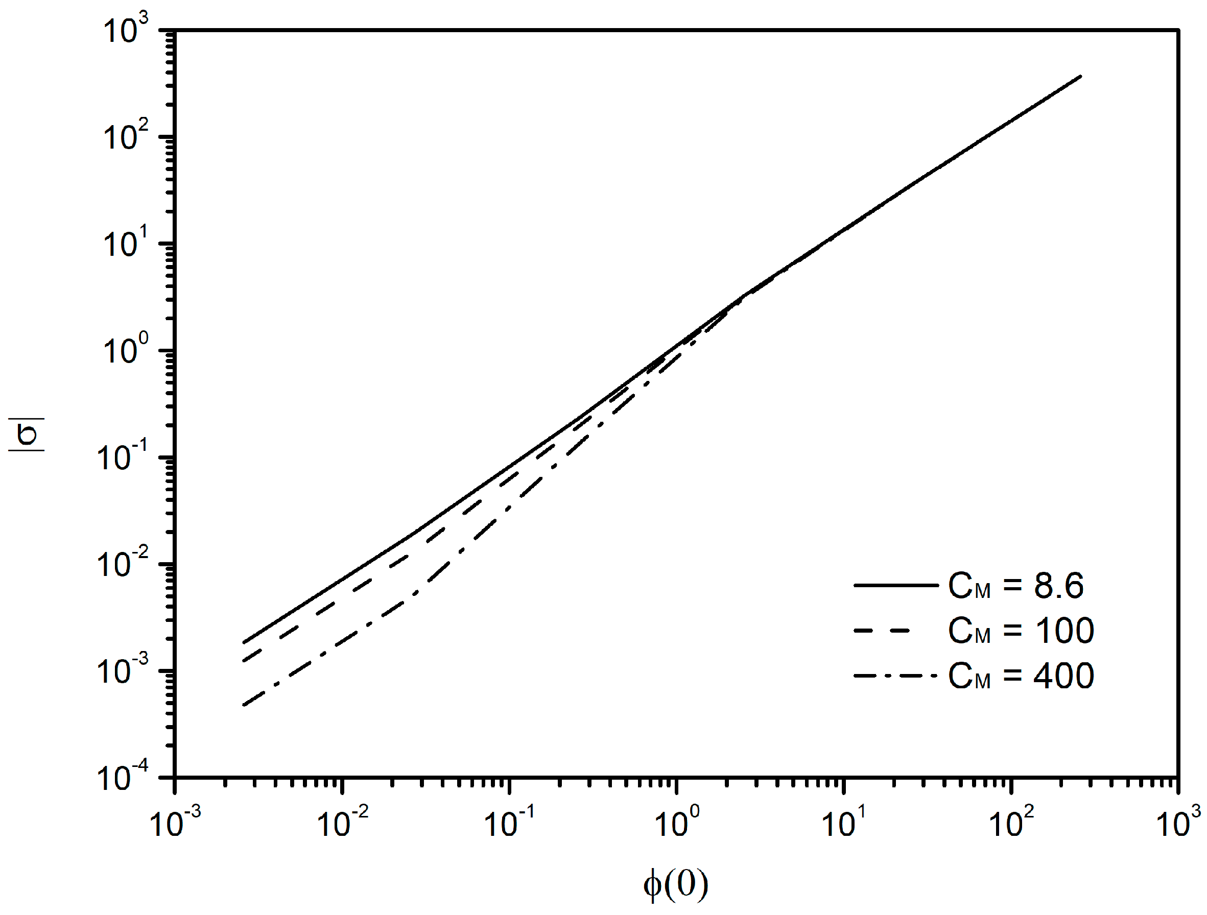
The distribution of the surface charge density as a function of is shown in Figure 3 for various concentrations considering the case of salty water, . As may be seen by comparing these results with the those from Reference [46], where no compact layer was considered, the deployment of the compact layer results in a reduced charge. Moreover, the charge is practically independent from the solution salt concentration.
As it may be observed, the relation (38) is different than Equation (34) due to linearized PNP equations or the electric models. However, it collapses to this upon linearization, i.e., for , something that can not be applied in general at the double layer. Now, the potential at the outer Helmholtz plane is
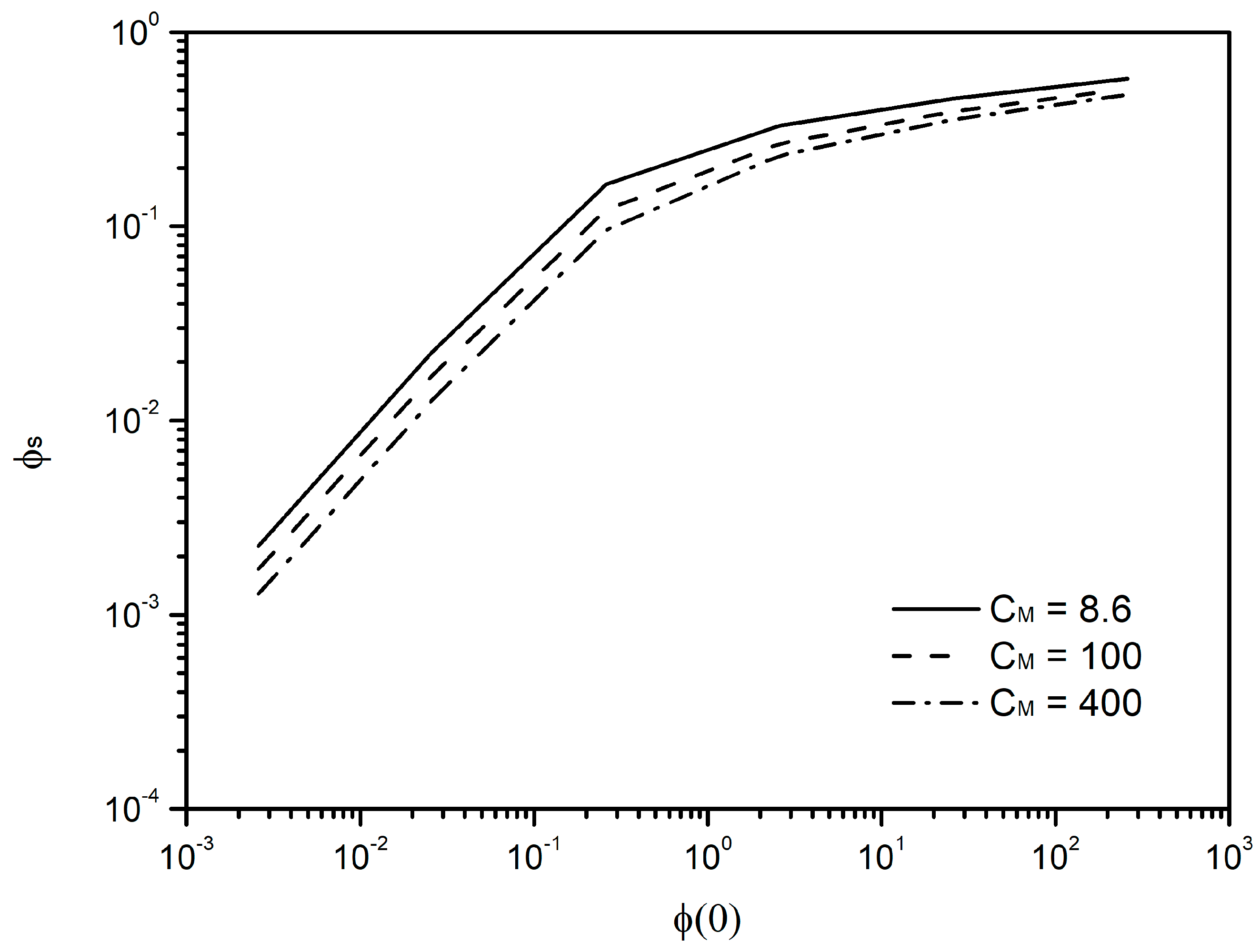
or
The potential at the outer Helmholtz plane is shown in Figure 4 as a function of for various concentrations considering the case of salty water, . As it can be observed, is scaled almost linear with for values up to 0.1 V. However, as is increased further, is saturated to values lower than 1 V independently of .
Now, the potential distribution along y in the diffuse layer for can be found from Equation (35) as
Thus, the electric field intensity inside the compact layer is given by
or
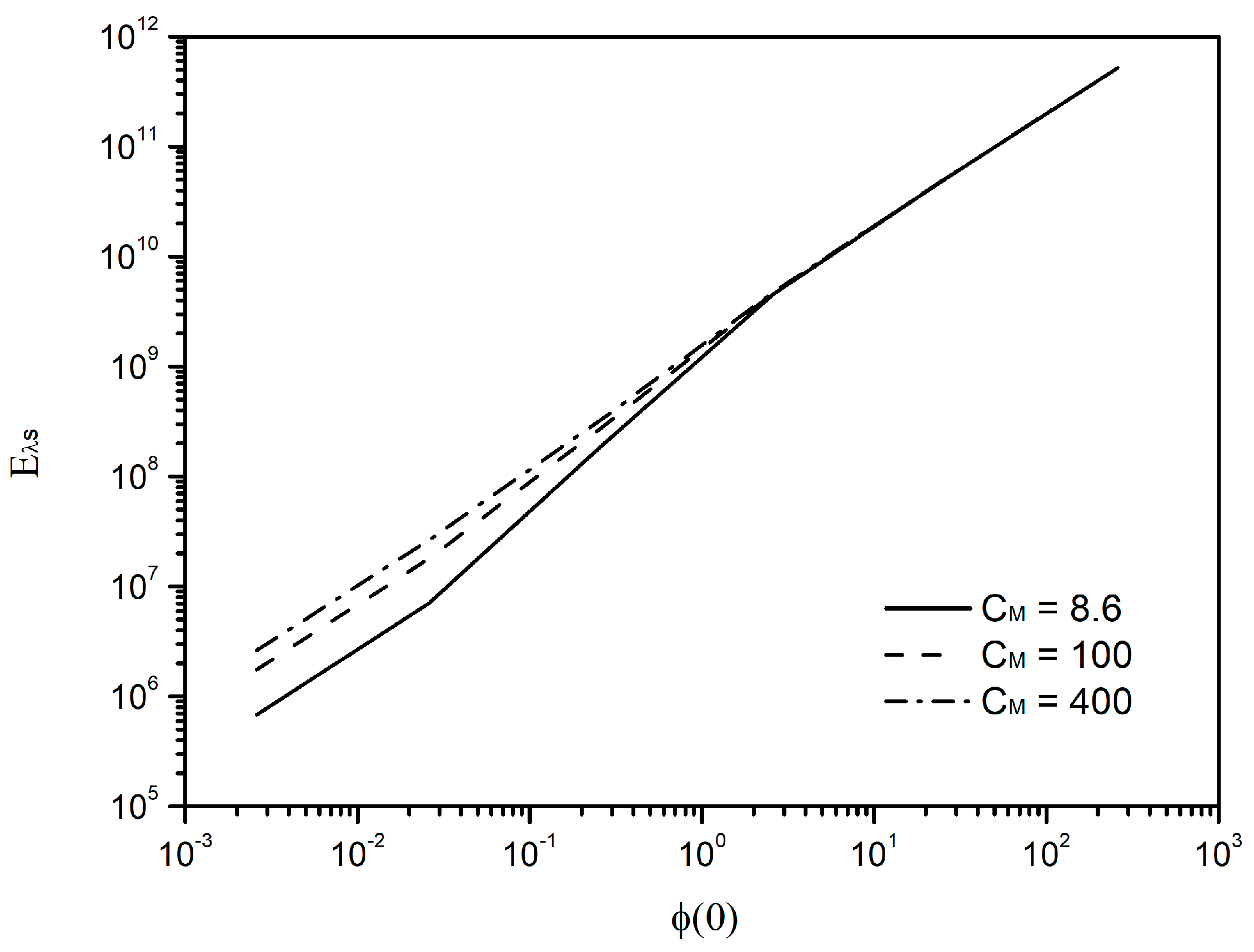
As it is observed from Figure 5 for the case of salty water, , the electric field intensity at the compact layer takes huge values independently of the ion concentration, especially as the potential increases.
5. Nonlinear PNP Solution
Starting from and setting Equation (3) in the form
and by subtracting, we have
The above Equation (46) can be transformed into the linear Equation (12) subject to . Since along the y-direction the ion concentration is changing, the decrease in the positive ion needs to correspond to the increase in the negative ion for their summary to be constant and equal to , i.e., .
This is valid throughout the duct width (for the case of salty water, ) when or , i.e., in the case of very weak external electric fields as already proved in Reference [46]. However, this is true only in the solution’s bulk as the applied potential increases and faults inside the double layer. Since we proved that the time scale of the problem is of the order of a second, we study the final equilibrium state of the ion drift. Similar to Section 3.3, we can assume that the final concentration profiles upon equilibrium that came after the solution of Equations (44)–(46) are of the form
and
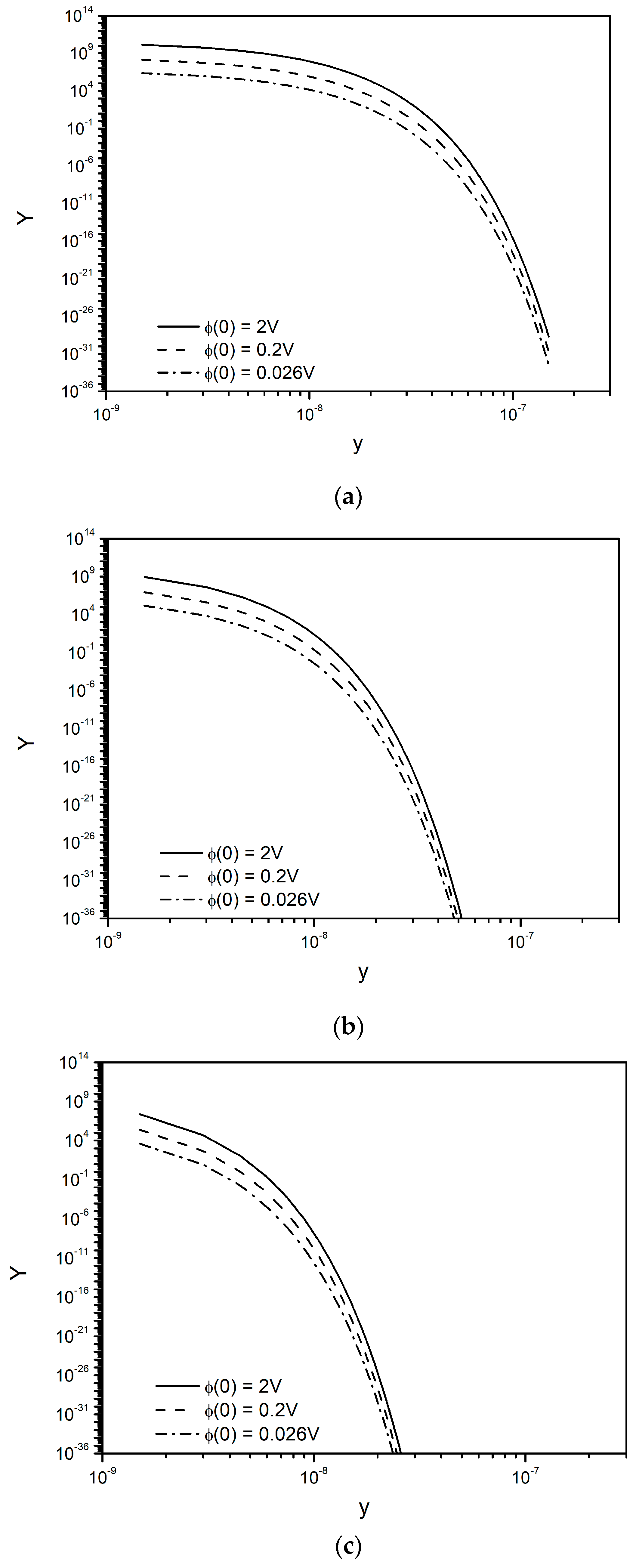
The effect of the nonlinearity can be investigated when a third term in the Taylor series of the exponential function, is considered. Then, for the additional term, it is
where , and .
Thus, from Equation (46) and by setting for the steady-state, it is
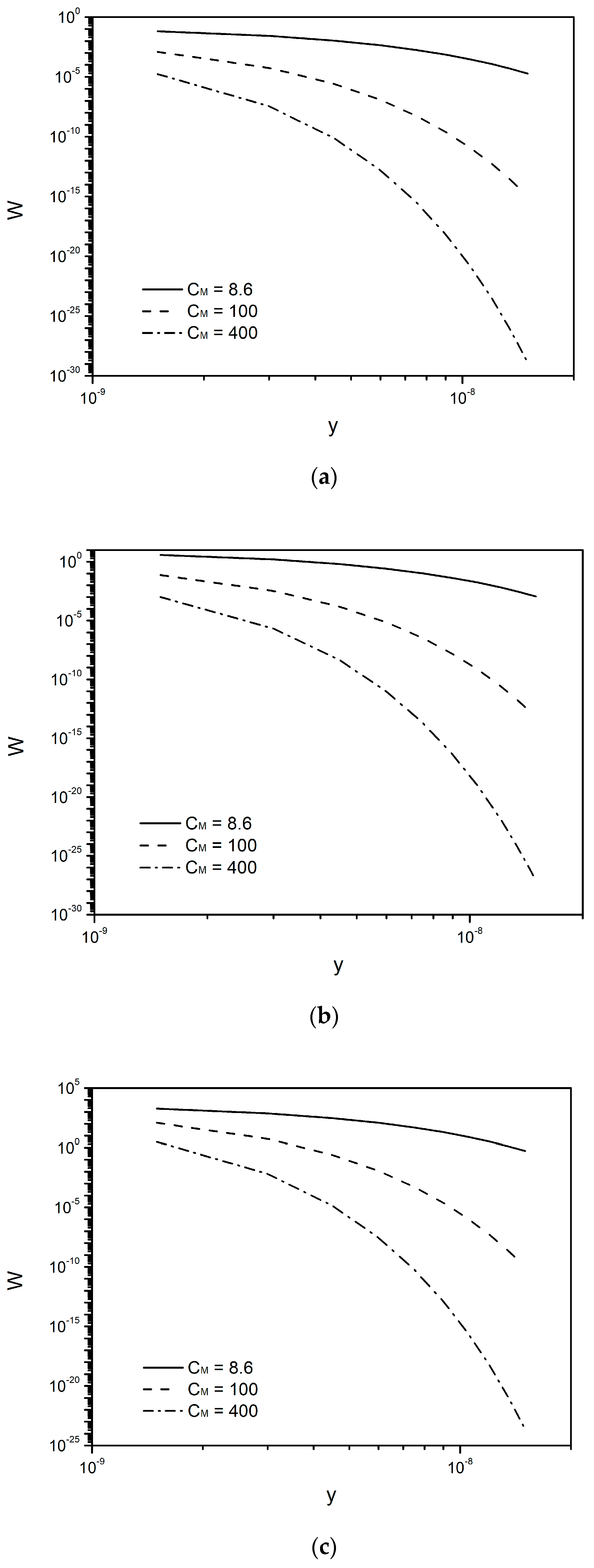
The shift of the linearity is due to W and Y. It will be useful to study their profiles along y for various potentials (for the case of salty water, ). In the range of 0.026, 0.2 and 2 V, concentrations are in the range of 8.6, 100 and 400 mol/m3 with a duct width of L = 0.015 m, while the effect of L is insignificant.
As it is observed in Figure 6 and Figure 7, only inside the compact layer can a deviation from linearity be encountered, while the difference is very negligible outside this layer as one would expect. Moreover, the width of the deviation is found to be inversely proportional to as it is also discussed in Reference [46].
6. Comparison with Experimental Results
The only available and relevant experimental data are from the capacitive deionization method and are obtained for the water desalination case. A typical duct width of the order L = 1.5 mm is proposed and constructors indicate a performance of about 65% for low salt concentrations. In a similar approach, the authors of Reference [40] succeeded in reducing an initial ion concentration of to the final concentration of with V = 0.4 V; thus, the electric charge that it is removed per surface area is about . This large ion drift can only be achieved by the existence of an electric field in the fluid bulk. This is due to the micropores in the capacitive deionization method. However, this is not possible here due to the non-Faradaic conditions to which our analysis refers. Clearly, the phenomenon of ion drift stops long before we have a noticeable reduction in ion in the bulk of the solution. This is due to the zeroing of the electric field in the bulk due to the creation of the double layer on the side walls of the duct. Thus, we need to continuously absorb the compact layer in order to permit additional ions to move close to the duct sidewalls. This can be conducted in an almost continuous way because as we showed, the time to reach the final equilibrium state is of the order of one second or less. This is equivalent to maintaining a non-zero electric field at the fluid’s bulk. This mechanism of ion removal from the salted water is discussed in Reference [37] since in this case, the solution had a constant electric field, which is impossible upon creation of the double layer, and in order for the electric field to exist, we have to continuously eliminate this layer. Thus, electric field existence in the duct is the crucial parameter to ensure that an efficient desalination can be achieved by this method. The absorption of the double layer replaces the porous electrodes and if achieved experimentally may be the solution for continuous desalination without the inevitable interruptions that must occur in capacitive deionization to discharge the electrodes.
7. Conclusions
This study examined the ion concentration, electric field, electric potential profiles and surface charge density inside a salt solution when it is under the effect of an external electric field as a function of time and position. The compact layer is discussed as it forms an additional mechanism to diminish the electric field in the bulk of the fluid. The conditions and the region where the linear approximation gives satisfactory results are examined.
The energy consumption of conventional methods using membranes is in the order of 0.30–2.11 kWh/m3, quite costly but provides desalination of a large scale. With a capacitive deionization method, we have a smaller energy consumption of about 0.2 kWh/m3. At present with this method, we can manage smaller amounts of water, and it can be used as a secondary desalination method. Research continues intensively on this method mainly with regard to electrodes in order to achieve greater absorbency. With the EID method, we have the same energy consumption, but we are exempt from the cost of electrodes.
The importance of maintaining a non-zero electric field in the fluid’s bulk is shown, which can only be succeeded by the continuous absorption of the double layer.
Author Contributions
Conceptualization, V.B.; methodology, V.B.; software, I.E.S.; investigation, V.B.; writing—original draft preparation, V.B.; writing—review and editing, I.E.S.; visualization, I.E.S. All authors have read and agreed to the published version of the manuscript.
Funding
This research received no external funding.
Institutional Review Board Statement
Not applicable.
Informed Consent Statement
Not applicable.
Data Availability Statement
Not applicable.
Conflicts of Interest
The authors declare no conflict of interest.
Nomenclature
| Concentration, mole/m3 | |
| μ | Mobility, |
| D | Diffusion coefficient, /s |
| J | Ionic flux, |
| i | Current density, |
| T | Absolute temperature, K |
| z | Number of overflow protons or electrons |
| E | Electric field intensity V/m |
| y | y-axis coordinate, m |
| L | Width of the duct, m |
| σ | Electric charge surface density C/m2 |
| C | Capacity, F |
| Greek symbols | |
| electric permittivity, F/m | |
| φ | Electric potential, V |
| ρ | Charge density, |
| υ | Velocity, m/s |
| ν | Dynamic viscosity, Pa s |
| σ | Surface charge density, C/m2 |
| Subscripts | |
| y | Along y-axis |
| bef | Before |
| after | After |
| Constants | |
Appendix A. General Theory of Ion Movement
It is supposed that a positive ion of concentration C+ is dissolved in a water solution that is flowing in the streamwise direction of a duct (Figure 1). Moreover, a uniform electric field of magnitude E is applied normal to the flow, and the corresponding force acting on the ions is
Then, the result is that ions start to drift. Thus, a spatial concentration distribution along the y-direction is formed, which causes the concentration gradient . The pseudoforce per ion due to this is given by the relation:
The negative sign indicates that the force direction is opposite to the concentration gradient direction, along the y-direction. Moreover, during the ion movement, a friction force also exists between the moving ion and the solvent. This force is opposite to the ion velocity , which is given approximately by the relation (we consider as usual the ion shape as a small sphere with radius r that moves with a small velocity inside a fluid of dynamic viscosity ν):
Quickly, equilibrium is established; thus,
By using Equations (A1)–(A3), the velocity can be found as
Appendix B. The RC Models—Time Scale
In Electrochemistry, there is an old theoretical approximation that when an electrolyte is under the effect of an external electric field, it is modeled as an effective electric circuit constituted by one capacitor and one resistance connected inline [52]. In the following, the most important models are reviewed.
Appendix B.1. Gouy-Chapman Model
The very first model used was attributed to Gouy–Chapman [52] in which only the diffuse layer that is formed from the ions’ confinement nearby the electrodes’ surface is considered. This thin layer can be simulated by a capacitor with a plate separation width: . Thus, the capacity per unit area is equal to . Since an additional capacitor is formed at the other wall of the duct, the total capacity per unit area is then
Assuming that the bulk of the solution is in an almost uniform initial ion concentration, the electric force due to the external electric field on the ions is fast balanced by the friction force, and their asymptotic velocity can be found from (A4) when for the positive ions as in . Their ionic flux is also given by , while is similarly given for the negative one. The electric current per unit surface is given by or substituting . Comparing this relationship with the Ohm’s law , the special conductivity is given by the relation . The resistance per unit surface is given by and, thus,
The time constant of the RC circuit determines that characteristic time of the phenomenon as
while is its practical duration according to the RC circuit theory. In the above Gouy–Chapman theory, only the diffuse layer and no compact layer is considered.
Appendix B.2. Stern’s Model
Assuming that ions have finite dimensions and, thus, that they can approach in an ionic radius distance to the walls of the duct that is of the order (further increased by the solvent molecules that surround the ion), the Stern model needs to be used. According to this model, the double layer is formed by two areas:
- The compact part that is simulated by a Helmholtz capacitor of effective width of the order of molecule that is almost constant. The term effective is due to the possibility that the solvent (i.e., the water here) may not be considered in this region as a continuous media, and the permittivity ε is considered to be similar to the fluid’s bulk. Thus, the width of the compact part may be considered the size of the ionic radius, i.e., [51], while in the present calculations, it is assumed to be equal to . Thus, the capacity of the compact part per unit area is given by .
- The diffuse layer that is simulated by a Gouy–Chapman-type capacitor with effective width of the diffuse part , and the known capacity per area unit is given by .
The above two capacitors are both inline connected and connected with the two capacitors existed at the other wall side (near the second electrode). The two electrodes constitute the Stern model [52]. Thus, the total capacity per surface unit is then
The time constant of the RC circuit of the Stern model is then
Appendix C. Solution of the Linear PNP Equation
Using the Laplace transformation in Equation (12) and assuming for the initial current density, we have
where
and is the |Laplace transformation of . The solution of Equation (A11) is of the form
where , and are constants. Due to antisymmetric conditions around the duct center at , it is , and, thus, , i.e.,
where
In order to determine the A constant, the Laplace transformed Poisson Equation (5) is used, , and integrated once:
where is a constant to be determined by considering the current density, , and it vanishes at the duct walls. Using Equation (12), the current density can be found as
While the Laplace transformed Equation (A17) reads as
and . Substituting and from Equations (A14) and (A16), respectively, the constant can be found as
Moreover, integrating Equation (A16) and using the antisymmetric condition, we find , and from Equation (A19):
The constant can be obtained by the boundary condition at from the transformed Equation (6), , when and are substituted by Equations (A20) and (A16) for . Thus, is found as
The Debye time is defined as and is of the order , while we are interested in system responses at higher time scales. From the Laplace transformation, , and it may be observed that for the function not to be zero as time increases, S should be less than a threshold value. Given that , it is found that and from Equation (A12), it appears that . Then,
Thus,
The inverse Laplace transformation of functions is and is and , respectively, resulting then in Equations (14)–(21).
References
- Setiawan, A.A.; Zhao, Y.; Nayar, C.V. Design, Economic analysis and environmental considerations of mini-grid hybrid power system with reverse osmosis desalination plant for remote areas. Renew. Energy 2009, 34, 374–383. [Google Scholar] [CrossRef]
- Cipollina, A.; Micale, G. Coupling sustainable energy with membrane distillation processes for seawater desalination. In Proceedings of the 2010 1st International Nuclear & Renewable Energy Conference (INREC), Amman, Jordan, 21–24 March 2010. [Google Scholar]
- García-Rodríguez, L. Renewable energy applications in desalination: State of the art. Sol. Energy 2003, 75, 381–393. [Google Scholar] [CrossRef]
- Wilf, M.; Awerbuch, L.; Bartels, C.; Mickley, M.; Pearce, G.; Voutchkov, N. The Guidebook to Membrane Desalination Technology. Reverse Osmosis, Nanofiltration and Hybrid Systems. Processes, Design, Applications; Balaban Desalination Publications: L’Aquila, Italy, 2011. [Google Scholar]
- Guoling, R.; Houjun, F. Technical Progress in Seawater Desalination Technology at Home and Abroad. China Water Wastewater 2008, 20, 86–90. [Google Scholar]
- Mathioulakis, E.; Belessiotis, V.; Delyannis, E. Desalination by using alternative energy: Review and state-of-the-art. Desalination 2007, 203, 346–365. [Google Scholar] [CrossRef]
- Mohamed, E.; Papadakis, G.; Mathioulakis, E.; Belessiotis, V. The effect of hydraulic energy recovery in a small sea water reverse osmosis desalination system; experimental and economical evaluation. Desalination 2005, 184, 241–246. [Google Scholar] [CrossRef]
- Mohamed, E.; Papadakis, G.; Mathioulakis, E.; Belessiotis, V. An experimental comparative study of the technical and economic performance of a small reverse osmosis desalination system equipped with an hydraulic energy recovery unit. Desalination 2006, 194, 239–250. [Google Scholar] [CrossRef]
- Mohamed, E.S.; Papadakis, G.; Mathioulakis, E.; Belessiotis, V. A direct coupled photovoltaic seawater reverse osmosis desalination system toward battery based systems—A technical and economical experimental comparative study. Desalination 2008, 221, 17–22. [Google Scholar] [CrossRef]
- Li, N.; Fane, A.; Winston, W.H.; Matsuura, T. Advanced Membrane Technology and Applications; Wiley: Hoboken, NJ, USA, 2008. [Google Scholar]
- Mezher, T.; Fath, H.; Abbas, Z.; Khalid, A. Techno-economic assessment and environmental impacts of desalination technologies. Desalination 2011, 266, 263–273. [Google Scholar] [CrossRef]
- Maerzke, K.A.; Siepmann, J.I. Effects of an Applied Electric Field on the Vapor−Liquid Equilibria of Water, Methanol, and Dimethyl Ether. J. Phys. Chem. B 2010, 114, 4261–4270. [Google Scholar] [CrossRef] [PubMed]
- Bakker, H.J. Structural Dynamics of Aqueous Salt Solutions. Chem. Rev. 2008, 108, 1456–1473. [Google Scholar] [CrossRef] [PubMed]
- Morro, A.; Drouot, R.; Maugin, G.A. Thermodynamics of Polyelectrolyte Solutions in an Electric Field. J. Non-Equilib. Thermodyn. 1985, 10, 131–144. [Google Scholar] [CrossRef]
- Wright, M. An Introduction to Aqueous Electrolyte Solutions; Wiley: Hoboken, NJ, USA, 2007. [Google Scholar]
- Gordon, M.J.; Huang, X.; Pentoney, S.L.; Zare, R.N. Capillary Electrophoresis. Science 1988, 242, 224–228. [Google Scholar] [CrossRef] [PubMed] [Green Version]
- Strathmann, H. Ion-Exchange Membrane Separation Processes; Elsevier: Amsterdam, The Netherlands, 2004; Volume 9. [Google Scholar]
- Ganzi, C.; Egozy, Y.; Giuffrida, A.; Jha, A. High purity water by electro-deionization. Ultrapure Water J. 1987, 4, 43–50. [Google Scholar]
- Tironi, I.; Sperb, R.; Smith, P.; van Gunsteren, W. A generalized reaction field method for molecular dynamics simulations. J. Chem. Phys. 1995, 102, 5451–5459. [Google Scholar] [CrossRef]
- Berendsen, H.; Postma, J.; van Gunsteren, W. Intermolecular Forces; Pullman, B., Ed.; Reidel Publishing Co.: Dordrecht, The Netherlands, 1981; pp. 331–342. [Google Scholar]
- Wulfsberg, G. Principles of Descriptive Inorganic Chemistry; University Science Books: South Orange, NJ, USA, 1991; pp. 23–31. [Google Scholar]
- Rasaiah, J.; Lynden-Bell, R. Computer simulation studies of the structure and dynamics of ions and non–polar solutes in water. Philos. Trans. R. Soc. Lond. Ser. A Math. Phys. Eng. Sci. 2001, 359, 1545–1574. [Google Scholar] [CrossRef]
- Belch, A.C.; Berkowitz, M.; McCammon, J.A. Solvation structure of a sodium chloride ion pair in water. J. Am. Chem. Soc. 1986, 108, 1755–1761. [Google Scholar] [CrossRef]
- Das, A.; Tembe, B. The pervasive solvent-separated sodium chloride ion pair in water-DMSO mixtures. Proc. Indian Acad. Sci. (Chem. Sci.) 1999, 111, 353–360. [Google Scholar]
- Murad, S. The role of external electric fields in enhancing ion mobility, drift velocity, and drift–diffusion rates in aqueous electrolyte solutions. J. Chem. Phys. 2011, 134, 114504. [Google Scholar] [CrossRef] [PubMed]
- Sheikholeslami, M.; Sheremet, M.A.; Shafee, A.; Li, Z. CVFEM approach for EHD flow of nanofluid through porous medium within a wavy chamber under the impacts of radiation and moving walls. J. Therm. Anal. Calorim. 2019, 138, 573–581. [Google Scholar] [CrossRef]
- Sofos, F.; Karakasidis, T.E.; Spetsiotis, D. Molecular dynamics simulations of ion separation in nano-channel water flows using an electric field. Mol. Simul. 2019, 45, 1395–1402. [Google Scholar] [CrossRef]
- Suss, M.E.; Porada, S.; Sun, X.; Biesheuvel, P.; Yoon, J.; Presser, V. Water desalination via capacitive deionization: What is it and what can we expect from it? Energy Environ. Sci. 2015, 8, 2296–2319. [Google Scholar] [CrossRef] [Green Version]
- Azamat, J. Functionalized Graphene Nanosheet as a Membrane for Water Desalination Using Applied Electric Fields: Insights from Molecular Dynamics Simulations. J. Phys. Chem. C 2016, 120, 23883–23891. [Google Scholar] [CrossRef]
- Drahushuk, L.W.; Strano, M.S. Mechanisms of Gas Permeation through Single Layer Graphene Membranes. Langmuir 2012, 28, 16671–16678. [Google Scholar] [CrossRef]
- Sun, C.; Boutilier, M.S.H.; Au, H.; Poesio, P.; Bai, B.; Karnik, R.; Hadjiconstantinou, N.G. Mechanisms of Molecular Permeation through Nanoporous Graphene Membranes. Langmuir 2014, 30, 675–682. [Google Scholar] [CrossRef] [PubMed]
- Cohen-Tanugi, D.; Grossman, J.C. Water Desalination across Nanoporous Graphene. Nano Lett. 2012, 12, 3602–3608. [Google Scholar] [CrossRef]
- Humplik, T.; Lee, J.; O’Hern, S.C.; A Fellman, B.; Baig, M.A.; Hassan, S.F.; Atieh, M.; Rahman, F.; Laoui, T.; Karnik, R.; et al. Nanostructured materials for water desalination. Nanotechnology 2011, 22, 292001. [Google Scholar] [CrossRef] [PubMed]
- Suk, M.E.; Aluru, N. Water Transport through Ultrathin Graphene. J. Phys. Chem. Lett. 2010, 1, 1590–1594. [Google Scholar] [CrossRef]
- Wang, E.; Karnik, R. Water Desalination: Graphene Cleans Up Water. Nat. Nanotechnol. 2012, 7, 552–554. [Google Scholar] [CrossRef] [PubMed]
- Ninos, G.; Bartzis, V.; Merlemis, N.; Sarris, I. Uncertainty quantification imlementations in human hemodynamic. Comput. Methods Programs Biomed. 2021, 203, 106021. [Google Scholar] [CrossRef] [PubMed]
- Bartzis, V.; Sarris, I.E. A theoretical model for salt ion drift due to electric field suitable to sea water desalination. Desalination 2020, 473, 114163. [Google Scholar] [CrossRef]
- Oren, Y. Capacitive deionization (CDI) for desalination and water treatment past, present and future (a review). Desalination 2008, 228, 10–29. [Google Scholar] [CrossRef]
- Choia, J.; Dorjib, P.; Shonb, H.; Honga, S. Applications of capacitive deionization: Desalination, softening, selective removal, and energy efficiency. Desalination 2019, 449, 118–130. [Google Scholar] [CrossRef]
- Minhas, M.; Jande, Y.; Kim, W. Hybrid Reverse Osmosis-Capacitive Deionization versus Two-Stage Reverse Osmosis: A Comparative Analysis. Chem. Eng. Technol. 2014, 37, 1137–1145. [Google Scholar] [CrossRef]
- Peters, P.B.; van Roij, R.; Bazant, M.; Biesheuvel, P. Analysis of electrolyte transport through charged nanopores. Phys. Rev. E 2016, 93, 053108. [Google Scholar] [CrossRef] [PubMed] [Green Version]
- Biesheuvel, P.M.; Bazant, M. Analysis of ionic conductance of carbon nanotubes. Phys. Rev. E 2016, 94, 050601. [Google Scholar] [CrossRef] [PubMed] [Green Version]
- Tsouris, C.; Mayes, R.; Kiggans, J.; Sharma, K.; Yiacoumi, S.; DePaoli, D.; Dai, S. Mesoporous carbon for capacitive deionization of saline water. Envirom. Sci. Tech. 2011, 45, 10243–10249. [Google Scholar] [CrossRef] [PubMed]
- He, F.; Biesheuvel, P.M.; Bazant, M.; Hatton, T.A. Theory of water treatment by capacitive deionization with redox active porous electrodes. Water Res. 2018, 132, 282. [Google Scholar] [CrossRef] [PubMed]
- Guyes, E.N.; Shocron, A.N.; Simakovski, A.; Biesheuvel, P.M.; Suss, M. A one dimensional model for water desalination by flow-through electrode capacitive deionization. Desalination 2017, 415, 8. [Google Scholar] [CrossRef] [Green Version]
- Bartzis, V.; Sarris, I.E. Electric field distribution and diffuse layer thickness study due to salt ion movement in water desalination. Desalination 2020, 490, 114549. [Google Scholar] [CrossRef]
- Atkins, P.; Paola, J. Atkin’s Physical Chemistry, 8th ed.; Oxford University Press: New York, NY, USA, 2006; Volume 5, pp. 136–169. [Google Scholar]
- Mortimer, R.G. Physical Chemistry, 3rd ed.; Elsevier: Amsterdam, The Netherlands, 2008; Volume 8, pp. 351–378. [Google Scholar]
- Brett, C.A.; Arett, A. Electrochemistry Principles, Methods, and Applications; Oxford University Press: New York, NY, USA, 1994. [Google Scholar]
- Debye, P.; Hückel, E. The theory of electrolytes. I. Lowering of freezing point and related phenomena. Phys. Z. 1923, 24, 185–206. [Google Scholar]
- Bonnefont, A.; Argoul, F.; Bazant, M. Analysis of diffuse-layer effects on time-dependent interfacial kinetics. J. Electroanal. Chem. 2001, 500, 52–61. [Google Scholar] [CrossRef]
- Bazant, M.; Thornton, K.; Ajdari, A. Diffuse-charge dynamics in electrochemical systems. Phys. Rev. E 2004, 70, 021506. [Google Scholar] [CrossRef] [PubMed] [Green Version]
- Biesheuvel, P.M.; Dykstra, J.E. The difference between Faradaic and Nonfaradaic processes in Electrochemistry. arXiv 2021, arXiv:1809.02930. [Google Scholar]
- Golovnev, A.; Trimper, S. Exact solution of the Poisson–Nernst–Planck equations in the linear regime. J. Chem. Phys. 2009, 131, 114903. [Google Scholar] [CrossRef] [PubMed]
- Nekrasov, S.A. Calculating the electrostatic field in the bulk of an aqueous solution. Russ. J. Phys. Chem. A 2012, 86, 1732–1735. [Google Scholar] [CrossRef]
- Han, J.-H.; Muralidhar, R.; Waser, R.; Bazant, M.Z. Resistive Switching in Aqueous Nanopores by Shock Electrodeposition. Electrochim. Acta 2016, 222, 370–375. [Google Scholar] [CrossRef] [Green Version]
Figure 1.
Flow configuration (a) and indicative salt ion distribution (b) of the present model.

Figure 2.
Time constant variation as a function of for various duct widths.

Figure 3.
Surface charge density dependance on at the outer Helmholtz plane for various .

Figure 4.
Potential dependance on at the outer Helmholtz plane for various .

Figure 5.
Electric field intensity inside the compact layer dependance on for various .

Figure 6.
Effect of the nonlinearity on W at and along for various .

Figure 7.
Effect of the nonlinearity on Y along for various at mol/m3 (a), mol/m3 (b) and mol/m3 (c).
Figure 7.
Effect of the nonlinearity on Y along for various at mol/m3 (a), mol/m3 (b) and mol/m3 (c).

Publisher’s Note: MDPI stays neutral with regard to jurisdictional claims in published maps and institutional affiliations. |
© 2021 by the authors. Licensee MDPI, Basel, Switzerland. This article is an open access article distributed under the terms and conditions of the Creative Commons Attribution (CC BY) license (https://creativecommons.org/licenses/by/4.0/).
Share and Cite
MDPI and ACS Style
Bartzis, V.; Sarris, I.E. Time Evolution Study of the Electric Field Distribution and Charge Density Due to Ion Movement in Salty Water. Water 2021, 13, 2185. https://doi.org/10.3390/w13162185
AMA Style
Bartzis V, Sarris IE. Time Evolution Study of the Electric Field Distribution and Charge Density Due to Ion Movement in Salty Water. Water. 2021; 13(16):2185. https://doi.org/10.3390/w13162185
Chicago/Turabian StyleBartzis, Vasileios, and Ioannis E. Sarris. 2021. "Time Evolution Study of the Electric Field Distribution and Charge Density Due to Ion Movement in Salty Water" Water 13, no. 16: 2185. https://doi.org/10.3390/w13162185
Note that from the first issue of 2016, this journal uses article numbers instead of page numbers. See further details here.