GIS, Multivariate Statistics Analysis and Health Risk Assessment of Water Supply Quality for Human Use in Central Mexico

Abstract

The spatial assessments of water supply quality from wells, springs, and surface bodies were performed during the dry and rainy seasons in six municipalities in the eastern regions of Michoacán (Central Mexico). Different physicochemical parameters were used to determine the supplies’ Water Quality Index (WQI); all of the communities presented good quality. The analysis indicates that many water quality parameters were within limits set by the international standards, showing levels of “excellent and good quality” according to WQI, mainly during the dry season (except at San Pedro Jácuaro and Irimbo communities in the rainy season). However, some sites showed “poor quality” and “unsuitable drinking water” related to low pH levels (<5) and high levels of turbidity, color, Fe, Al, Mn, and arsenic. Multivariate statistical analysis techniques (Principal Component and Hierarchical Cluster) and geographic information system (GIS) identify potential sources of water pollution and estimate the geographic extension of parameters with negative effects on human health (mainly in communities without sampling). According to multivariate analysis, the Na⁺/K⁺ ratio and water temperature (22–42 °C) in various sites suggest that the WQI values were affected by geological and geothermal conditions and physical changes between seasons, but were not from anthropogenic activity. The GIS established predictions about the probable spatial distribution of arsenic levels, pH, temperature, acidity, and hardness in the study area, which provides valuable information on these parameters in the communities where the sampling was not carried out. The health risk assessment for dermal contact and ingestion showed that the noncancer risk level exceeded the recommended criteria (HQ > 1) in the rainy season for three target groups. At the same time, the carcinogenic risk (1 × 10⁻³) exceeded the acceptability criterion in the rainy season, which suggests that the As mainly represents a threat to the health of adults, children, and infants.

1. Introduction

Groundwater constitutes 97 percent of the global freshwater supply and is a significant source in several highly populated regions. The polluted groundwater could contribute to endemic diseases and, historically, has been poorly treated or untreated to make it safe for drinking, playing a highly significant role in human exposure to a wide variety of pollutants. As a result, monitoring and controlling groundwater quality must be a priority, particularly when the contamination is associated with human activities, to ensure public health [1,2]. Reports indicate that several natural and/or anthropogenic pollutants in groundwater and surface water can significantly affect human health. The presence of arsenic (As) in drinking water produces skin and other types of cancer (e.g., lung, bladder, and kidney), peripheral vascular disease, melanosis (abnormal black-brown pigmentation of the skin), hyperkeratosis (thickening of the soles of the feet), or gangrene [1,3]. Fluoride (F⁻) is associated with dental and skeletal fluorosis [4]. Selenium (Se) causes loss of hair and fingernails, finger deformities, skin lesions, tooth decay, and neurological disorders, even at low concentrations [5]. Nitrate (NO₃⁻), the main nitrogen compound in groundwater, causes methemoglobinemia in bottle-fed infants, which includes symptoms such as lethargy, shortness of breath, and bluish skin color (also named blue baby syndrome) [1].

Some studies have reported that chronic exposure to low concentrations of metals (e.g., Cr, Cd, Pb) might cause kidney damage and chronic kidney disease (CKD) (cadmium, lead, mercury, copper, nickel, uranium, arsenic, iron, mercury, bismuth, and chromium are the main nephrotoxic heavy metals that can cause tubular damage and glomerulopathies) [6,7,8,9,10]. In addition, high arsenic levels in drinking water are related to increased mortality associated with CKD [11].

Various approaches or data analysis tools have been used to find a relationship between the physicochemical parameters of the water of underground and surface bodies of human supply, its quality, the origin of the sources of contamination, and the potential effect on the health of the exposed populations. Studies with these diverse approaches have contributed to the development of different water quality indices and the support of multivariate statistical methods and geographic information systems (GIS). Numerous water quality indices (WQI) have been formulated worldwide based on the WQI developed by the U.S. National Sanitation Foundation (NSFWQI). The NSFWQI was designed to provide a standardized method for comparing the water quality of various water sources based on nine water quality parameters that have implications for human health, such as temperature, pH, dissolved oxygen, turbidity, fecal coliforms, biochemical oxygen demand, total phosphates, nitrates, and total solids. According to the NSFWQI method, the water quality categories are defined as excellent, good, medium, bad, and very bad [12]. Kawo et al. [13] studied the suitability of groundwater for consumption and irrigation in the Modjo river basin, Central Ethiopia, and generated the spatial variation information of cations and anions using inverse distance weighted IDW interpolation in GIS. Jha et al. [14] proposed a hybrid framework that integrates fuzzy logic with GQI-based GIS to assess groundwater quality and its spatial variability in a hard rock terrain of southern India using ten salient groundwater quality parameters measured during the pre- and post-monsoon seasons. Nnorom et al. [15] investigated applying different multivariate statistical approaches to assess the origin of pollutants in water bodies in southeastern Nigeria, obtaining a better understanding of water quality and possible sources that affect the studied system.

Furthermore, an important aspect of the study of water quality is estimating the potential risk associated with contact and ingestion of water. Moldovan et al. [16] studied water quality and the possible risk of groundwater ingestion in Karstic Springs in south-eastern Romania. Their findings indicate heavy metals in all springs and a possible noncancer risk from nitrates in adults and children. Similarly, Hussain et al. [17] estimated the health risk from heavy metals in drinking water and reported that Lahore, Vehari, Jhang, and Multan, Pakistan, exceed the safe limits of the health risk index for metals such as Cr, Ni, and As.

The high incidence of CKD in this region of Central Mexico has increased interest in assessing drinking water supply quality in the area, mainly where most CKD cases have been allocated (e.g., Ciudad Hidalgo and Zinapécuaro). Groundwater in Ciudad Hidalgo reports a high concentration of arsenic, which could contribute to the development of CKD among individuals in the region [18,19,20,21]. Nevertheless, relatively little knowledge about the water quality in other communities of the region compromises the population’s health and assesses how inhabitants of this area have adverse health effects from environmental pollutants.

The objectives of this study were (i) evaluate water quality with the Water Quality Index (WQI) in six municipalities in eastern Michoacán during the dry and rainy seasons. For this, multivariate statistical techniques (Principal Component Analysis and Hierarchical Cluster Analysis) were integrated to identify possible sources of contamination that influence the chemical composition of the water, and thereby establish predictions for the distribution of pollutant levels in the study area; (ii) estimate noncarcinogenic and cancer human health risk potential due to dermal contact and ingestion of water. The information generated in this study is essential for the monitoring, management, and sustainability of the water bodies in this region of Mexico. In addition, these data are expected to guide future research to help implement government policies to protect the population’s health and adequate management of water resources.

2. Materials and Methods

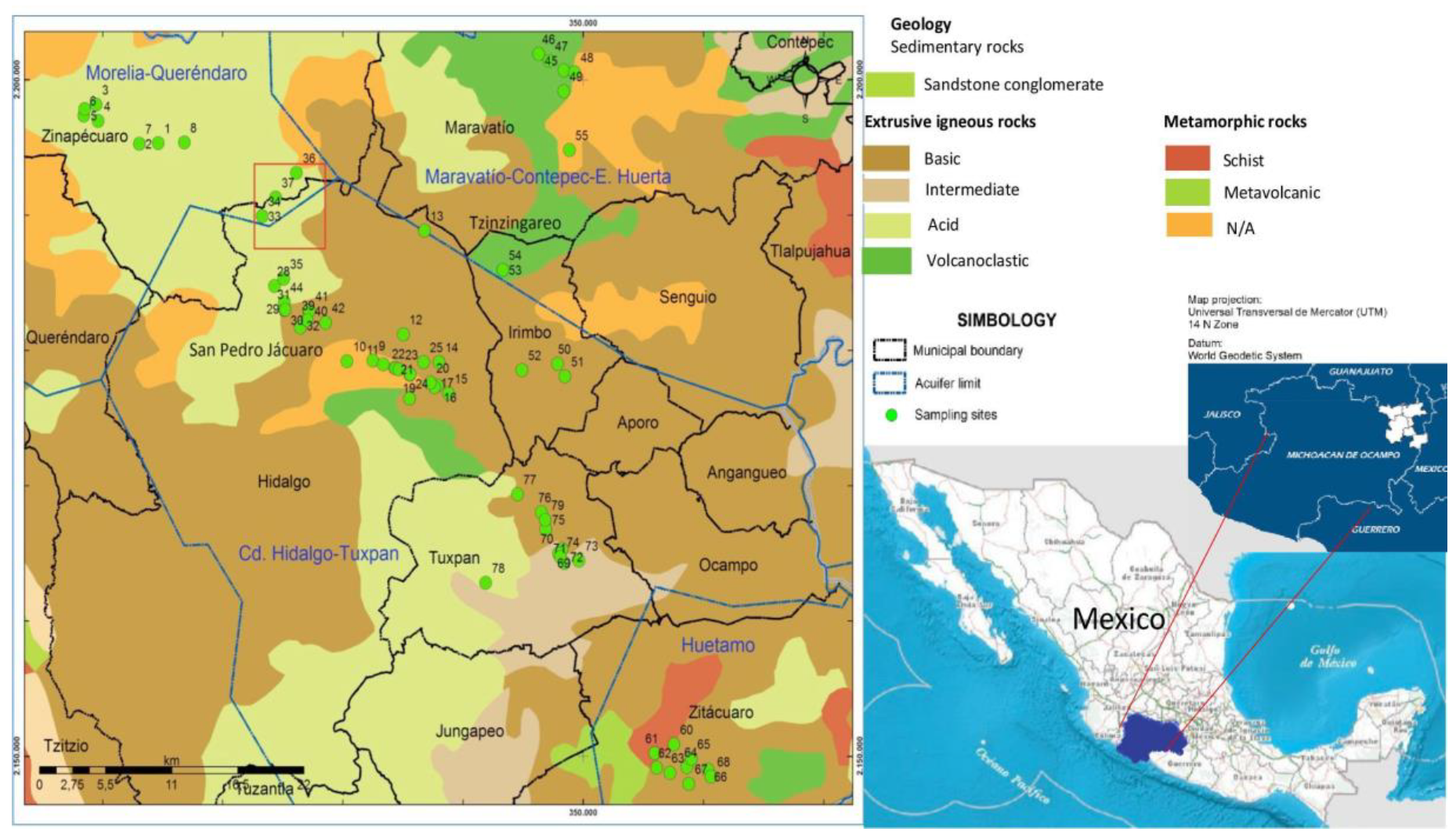
2.1. Study Area

The study area is located in Central Mexico (eastern Michoacán and Cuitzeo regions) inside 19°53′ and 19°26′ north latitude and 100°50′ and 100°21′ west longitude, with altitude ranging between 1727–2898 m above sea level (M.A.S.L.). The complete list of municipalities considered in the sampling campaigns and their geographical coordinates are contained in Table S1 of the Supplementary Materials. The study area is part of the Cutzamala, Lerma–Toluca, and Pátzcuaro–Cuitzeo–Yuridia hydric basins [22] and includes the “Los Azufres” geothermal field. The geothermal field is located within Zinapécuaro (ZIN) and Ciudad Hidalgo (HID) municipalities and has fifteen deep exploratory and production wells in a 30 km² area, which could influence drinking water quality and its physical and chemical characteristics, in particular those related to adverse effects on human health [23].

2.2. Water Sampling Sites

Water sampling was carried out during the dry (October 2012 to May 2013) and rainy (July to October 2013) seasons. Sampling sites corresponded to drinking water supply sources whose number varied by municipality and season (n = 69 and n = 65 in dry and rainy seasons, respectively). Figure 1 shows the sampling sites’ geographical locations, the distribution and extent of geological characteristics, and the extent of principal aquifers in the study area.

Most sampling sites corresponded to sources or reservoirs and springs drinking water supply. Some surface water samples from artificial and natural lagoons (e.g., Laguna Verde and Laguna Larga) and samples from water reservoirs intended for injection into the geothermal field were also taken. These lagoons and tanks of water for injection are within the area of activity of the “Los Azufres” geothermal field, corresponding to extraction and condensation water obtained from underground sources of steam during the production of electric energy. The condensed water is deposited in artificial lagoons and is injected into the subsoil [22,23]. Sampling, preservation requirements, and analysis time for each parameter were performed according to Standard Methods [24].

2.3. Physicochemical Water Quality Parameters

For field analysis, a multiparameter device (HANNA Instruments, model HI9828, Woonsocket, RI, USA) was used to collect data for pH, temperature, electric conductivity (EC), total dissolved solids (TDS), and dissolved oxygen (DO). In addition, GPS equipment (Garmin, eTrex-H, Olathe, KS, USA) was used to collect latitude, longitude, and altitude for every sampling site. The water quality parameters evaluated in the laboratory are shown in Table S2, along with information on the analysis methods and the equipment employed. The procedures followed validation protocols and quality control established in the Standard Methods to ensure the reliability of the results [24].

2.4. Water Quality Index

The Water Quality Index (WQI) was estimated for all water samples of the sites and municipalities (seasonal mean), according to the methodology reported by Şener et al. [12]. In their study, diverse parameters (e.g., pH, COD, sodium, calcium, magnesium, chloride, nitrate, sulfate, chromium, lead, and manganese) adversely affect human health (Table S3). In addition, we also included temperature, aluminum, and arsenic. Therefore, in agreement with these authors, the calculated WQI values have the following categories: excellent (<50); good (50–100); poor (100–200); very poor (200–300); unsuitable for drinking (>300).

From WQI, we could identify those parameters with a significant influence on the index itself. For this, the effective weights (E_wi) for each water quality parameter were calculated using Equation (1) [25]:

$${\mathbf{E}}_{\mathbf{w}\mathit{i}}=\frac{{\mathrm{SI}}_i}{\mathrm{WQI}}\times 100$$

(1)

where (SI_i) is the subindex of the ith parameter, WQI is each municipality’s overall Water Quality Index, and the result is multiplied by 100.

2.5. Statistical Analysis

A descriptive statistical analysis of results, including mean, standard deviation, and maximum and minimum values, was realized for all sites, municipality, and season water samples. The results were obtained from San Pedro Jácuaro (SPJ), a community of the HID municipality. The data were treated as an independent group because the site is close to the “Los Azufres” geothermal field. Likely, this geothermal field has a more substantial influence on the drinking water supply characteristics of SPJ.

Because ninety-four percent of the data did not follow a normal distribution, nonparametric tests allowed the analysis of the results. A multiple comparisons analysis was conducted for the different parameters to test the variation between municipalities for each season using the Kruskal–Wallis test. In addition, the comparisons between seasons were performed by contrasting the medians of two datasets for the same municipalities with the Mann–Whitney (Wilcoxon) test. The Kruskal–Wallis and Mann–Whitney test were mainly employed in result analysis from the Geographical and seasonal comparison section. When a statistical difference is mentioned in the text, at least one p-value, <0.05, was determined.

Lastly, a correlation analysis of seasonal sampling for each municipality and the entire dataset during dry and rainy seasons with Spearman (rs) correlation coefficients established the degree of association between physicochemical parameters, suggesting their origin and possible common sources. In the analysis, only samples from drinking water supply sources were considered.

2.6. Principal Component Analysis and Hierarchical Cluster Analysis

The principal component analysis (PCA) suggested probable sources of water pollutants and their associated study parameters for determining differences and similarities between sampling sites. As a requirement of multivariate tests, a logarithmic transformation allowed a normal distribution of data variables [25]. The standardization achievement minimizes differences in measurement units and variance and yields dimensionless data [26]. The absolute load values of >0.75, 0.75 to 0.50, and 0.50 to 0.30 were termed as “strong”, “moderate”, and “weak”, respectively [27]. The PCA contributed to explain the total variation (%), based on components with eigenvalues criterion (>1) and using varimax rotation for better interpretation of the results, and reduced the number of variables with the highest significance. The PCA was applied to the complete set of results from the study area by season.

Agglomerative hierarchical cluster analysis (HCA) set standardized data, employing Ward’s and Euclidean squared distance methods [28]. The application of HCA contributed to finding similarities and the identification of sampling site groups for each season. For this analysis, the data from all sites, including lagoons and injection water, were included—the statistical analysis employed Statistica 10^® (StatSoft, Tulsa, OK, USA) and Centurion XV.11^® software (Statpoint Technologies, Inc., The Plains, VA, USA).

2.7. Geographic Information System

Geographic information systems (GIS) facilitated the spatial distribution of water quality parameter analysis for the study area. Kriging spatial interpolation of the water quality parameters data was employed using ArcGIS 10^® software(ESRI, Redlands, CA, USA) with the Geostatistical Analyst extension [29,30]. Attributing weak and strong weights to the furthest and closest samples, respectively, facilitated the analysis [31]. The kriging method simulation was conducted in independent seasons with variables data related to potential adverse effects on human health (e.g., arsenic, pH, temperature, and hardness). Each sampling site and coordinates X, Y, and Z were used for spatial georeferencing within the software. The total area covered was 1600 km², with the center located at HID urban area. The geographical boundaries of the six municipalities were determined using a digital elevation model (DEM). Based on the topography of the study area, the boundaries modification defined a polygon covering only sampling sites. This procedure produced a raster output with the least mean square error, optimizing the value of the predictive model.

2.8. Health Risk Assessment

In the present study, a noncarcinogenic and carcinogenic health risk posed by hazardous elements is assumed through the use and consumption of groundwater and surface water in the study area. Although the water is used mainly for domestic activities, since it is customary to consume bottled water, it cannot be ruled out that some communities with difficult access to quality drinking water can use boiled water for drinking. Therefore, consumption via oral ingestion was considered.

2.8.1. Noncancer Risk

The average daily dose (ADD) for dermal contact and ingestion was calculated for three target groups according to the following equations:

$${\mathrm{ADD}}_{\mathrm{dermal}}=\mathrm{C}·{\mathrm{K}}_{\mathrm{p}}·{ \mathrm{S}}_{\mathrm{A}}·\frac{\mathrm{ED}·\mathrm{EF}·\mathrm{ET}·\mathrm{CF}}{\mathrm{BW}·\mathrm{AT}}$$

(2)

$${\mathrm{ADD}}_{\mathrm{ingestion}}=\frac{\mathrm{C}·\mathrm{IR}·\mathrm{ED}·\mathrm{EF}}{\mathrm{BW}·\mathrm{AT}}$$

(3)

where ADD is the average daily dose during the exposure through dermal contact and ingestion of water (mg/kg-day), C is the concentration of contaminant in water (mg/L), K_p is the skin permeability coefficient in water (0.001 cm/h), S_A is body surface areas (cm²), ET is the exposure time (0.6 h/day), CF is a unit conversion factor (0.001 L/cm³), IR is water ingestion rate (L/day), ED is exposure duration (years), EF is exposure frequency (365 days/years), BW is body weight (kg), and AT is the average lifetime (days) (

Table 1. Input data is used to calculate noncarcinogenic human health risk due to anions, metals, and toxic elements exposure through dermal contact and water ingestion [32,33].

		Adults (>65 Years)	Children (6–11 Years)	Infants (6–12 Months)
Body surface area (SA)	(cm2)	19,800 *	10,800	4500
Average ingestion of water (IR)	(L/d)	1.046	0.414	0.36
Exposure duration (ED)	(years)	65	11	1
Average body weight (BW)	(kg)	80	31.8	9.2
Average lifetime (AT)	(days)	23,725	4015	365

* Mean for adult males and females.

).

The HQ is the ratio between the calculated average daily dose (ADD) of chemicals to the dermal and oral reference dose (RfD, mg/ kg-day) that indicates the daily exposure to which the human population could be continually exposed over a lifetime without an appreciable risk of deleterious effects. The hazard quotients (HQ_ingestion and HQ_dermal) are calculated through dermal contact and ingestion pathways, respectively:

$$\mathrm{H}\mathrm{Q}=\frac{\mathrm{A}\mathrm{D}\mathrm{D}}{\mathrm{R}\mathrm{f}\mathrm{D}}$$

(4)

The exposed population is assumed to be safe when HQ is lower than 1. Additionally, the HI is defined as the potential noncarcinogenic health risk caused by different contaminants present in water bodies. It was calculated using the following equation:

$$\mathrm{H}\mathrm{I}={\displaystyle \sum }_{i=1}^n\mathrm{H}\mathrm{Q}$$

(5)

where HI value < 1 means the exposed population is not expected to experience hazardous health impacts. On the other hand, HI value > 1 means there is a possibility of noncarcinogenic health risks to the local people of the study area [34].

2.8.2. Cancer Risk

The probable cancer risks due to exposure to a specified dose of heavy metal in drinking water can be computed using the ILCR. The ILCR is defined as the cumulative probability of developing cancer over a lifetime due to exposure to a potential carcinogen. The following equation is commonly used for the calculation of the lifetime cancer risk:

$$\mathrm{I}\mathrm{L}\mathrm{C}\mathrm{R}=\mathrm{C}\mathrm{D}\mathrm{I}·\mathrm{C}\mathrm{S}\mathrm{F}$$

(6)

CDI is expressed as the average daily dose of elements through dermal contact and ingestion pathways, and CSF is the cancer slope factor and is defined as the risk generated by an average lifetime amount of one mg/kg/day of carcinogen chemical and is contaminant specific (

Table 2. Dermal and oral reference doses (RfD) and cancer slope factor (CSF).

Chemical	RfD Dermal (mg/kg-day)	RfD Ingestion (mg/kg-day)	Cancer Slope Factor (mg/kg-day)
Ba	1.4 × 10−2 a	7.0 × 10−2 a	NE
Cr	1.5 × 10−5 a	3.0 × 10−3 a	4.2 × 10−1 c
Cd	5.0 × 10−6 a	5.0 × 10−4 a	15c
Pb	4.2 × 10−4 a	1.4 × 10−3 a	8.5 × 10−3 c
As	1.23 × 10−4 b	3 × 10−4 b	1.5 d
Mn	8.0 × 10−4 a	2.0 × 10−2 a	NE
Ni	5.4 × 10−3 a	2.0 × 10−2 a	9.1 × 10−1 c

^a Tripathee et al. [36], ^b Li et al. [37], ^c OEHHA [38]; ^d USEPA IRIS [39]; NE: not established.

). The permissible limits are 10⁻⁶ and <10⁻⁴ for single carcinogenic and multielement carcinogens [35].

3. Results

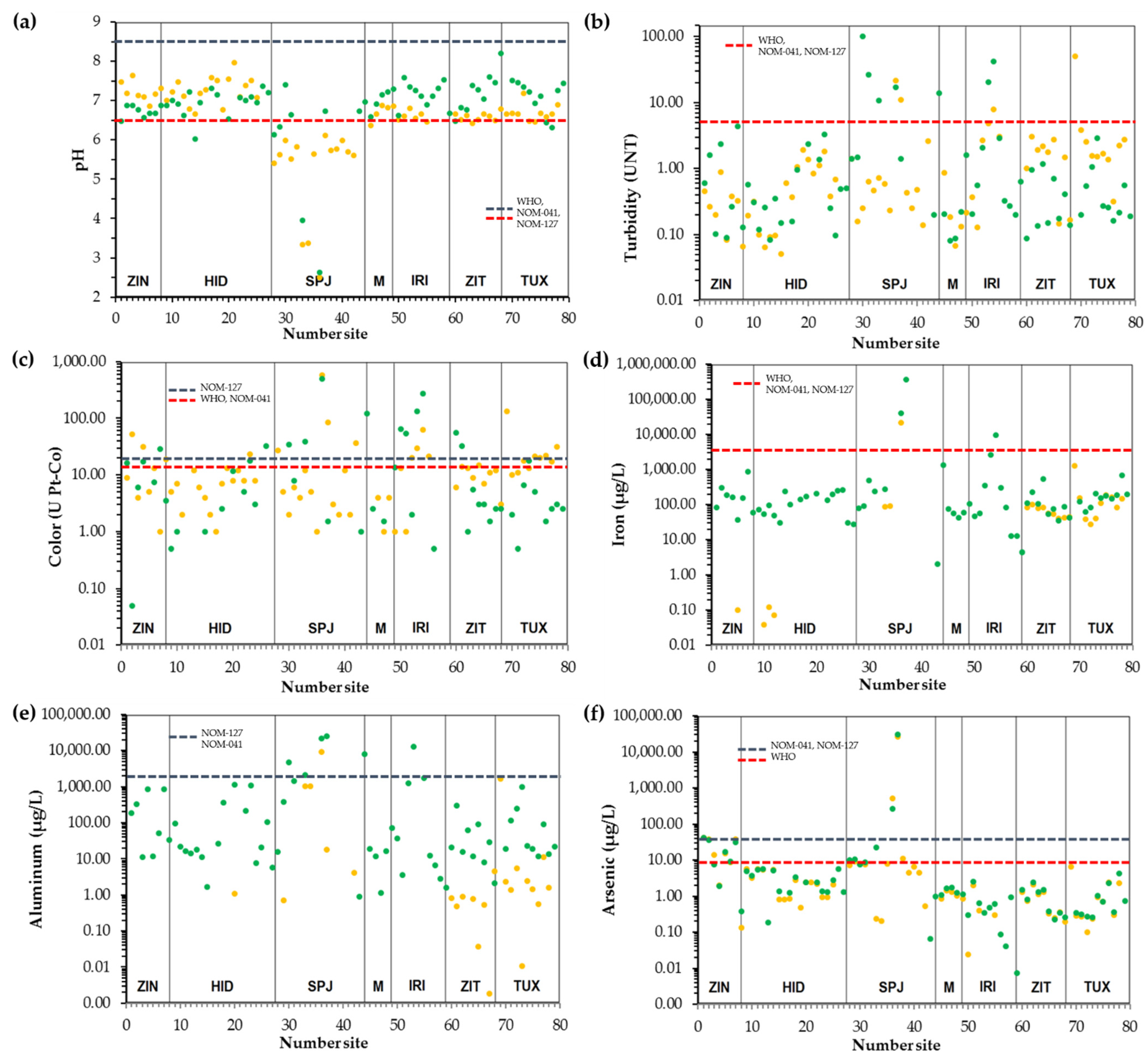
3.1. Water Quality Parameters

The descriptive statistical analysis results are presented in

Table 3. Descriptive statistics for water quality parameters by season.

Parameter	Units	Dry Season						Rainy Season						WHO [40], NOM-041 [41]; NOM-127 [42]
		n	Mean	SD	Median	Max	Min	n	Mean	SD	Median	Max	Min
pH	PU	68	6.62	0.81	6.66	7.96	3.33	54	6.95	0.55	6.96	8.21	3.95	6.5–8.5
EC	µS/cm	68	243.25	115.27	224.00	688.00	70.00	54	234.64	116.93	215.00	641.00	12.00	-
Temperature	°C	68	20.43	3.70	19.79	31.49	11.80	54	20.61	3.42	20.01	32.12	15.46	-
TDS	mg/L	68	123.72	59.61	113.00	344.00	35.00	54	113.70	59.88	106.00	321.00	6.00	500–1000
DO	mg/L	55	5.23	1.48	5.24	7.81	2.19	54	4.44	1.48	3.73	7.37	1.44	-
Turbidity	NTU	68	1.85	6.17	0.59	50.80	0.05	54	4.05	14.07	0.33	100.12	0.08	5
Color	Pt–Co	65	14.05	19.10	9.00	134.00	1.00	42	18.57	45.45	3.00	270.00	0.05	15–20
Acidity	mg/L	68	10.12	12.34	5.01	50.00	2.43	54	18.19	13.36	15.49	75.09	2.38	-
Alkalinity	mg/L	68	112.15	54.23	101.48	337.68	41.67	53	109.21	63.00	99.60	351.44	4.32	300
Hardness	mg/L	55	88.39	49.13	75.66	281.25	25.53	52	89.32	53.16	80.52	275.62	0.21	200–500
COD	mg/L	40	9.25	38.43	2.60	245.52	0.20	52	5.06	6.76	2.95	45.65	0.05	-
BOD5	mg/L	2	3.70	2.12	3.70	5.20	2.20	7	11.52	9.34	0.850	23.50	0.035	-
Li+	mg/L	68	B.D.L.	-	-	-	-	1	0.16	-	-	-	-	-
Na+	mg/L	68	17.17	9.49	14.45	53.87	4.77	52	17.75	10.12	15.17	55.20	5.73	200
NH4+	mg/L	68	B.D.L.	-	-	-	-	4	1.63	2.93	0.24	6.02	0.03	-
K+	mg/L	68	5.68	5.23	3.83	32.62	1.72	48	5.05	5.38	3.01	25.69	1.03	-
Ca+2	mg/L	68	16.57	10.16	12.52	49.21	3.26	53	16.56	10.07	12.73	46.82	3.37	75
Mg+2	mg/L	68	11.40	7.11	9.92	42.85	0.60	52	12.37	7.57	10.80	43.43	2.85	50
F−	mg/L	1	0.35	-	-	-	-	32	0.19	0.10	0.17	0.44	0.09	0.7–1.50
Cl−	mg/L	68	3.76	5.39	1.89	34.11	0.48	51	4.40	7.04	2.01	42.59	0.35	250
NO2−	mg/L	68	B.D.L.	-	-	-	-	54	B.D.L.	-	-	-	-	0.165–3
Br−	mg/L	68	B.D.L.	-	-	-	-	1	0.92	-	-	-	-	-
NO3−	mg/L	55	9.93	16.49	4.19	103.59	0.06	52	10.23	19.55	3.72	137.33	0.40	44–50
PO4−3	mg/L	4	0.75	0.48	0.56	1.45	0.44	2	3.66	2.91	3.66	5.72	1.59	-
SO4−2	mg/L	63	16.37	17.64	9.81	89.75	0.15	52	16.43	17.77	8.85	85.37	0.20	250–400
Ba	µg L−1	59	20.32	31.92	10.28	176.18	0.01	54	27.97	50.24	10.89	224.22	0.09	700
Cr	µg L−1	55	1.05	1.17	0.56	5.23	0.02	54	8.37	7.36	7.57	46.30	0.14	50
Fe	µg L−1	36	78.20	212.24	32.93	1274.08	0.01	54	342.94	1216.58	109.79	9402.31	2.10	300
Cu	µg L−1	54	0.88	1.05	0.49	5.15	0.01	54	2.68	4.49	1.74	35.67	0.01	1000–2000
Zn	µg L−1	40	15.45	51.46	1.60	236.00	0.01	54	26.18	11.51	2.68	68.78	0.35	3000–5000
Cd	µg L−1	50	0.04	0.23	0.00	1.66	0.00004	50	0.05	0.01	0.004	0.10	0.0003	3–5
Al	µg L−1	21	79.52	355.76	1.40	1632.17	0.002	53	516.84	1988.20	22.37	12793.08	0.90	200
Pb	µg L−1	38	0.42	2.48	0.02	15.31	0.001	50	0.28	0.42	0.14	2.63	0.002	10–25
As	µg L−1	52	4.40	9.25	1.20	42.13	0.024	54	131.55	8.17	1.33	40.76	0.01	10–50
Sb	µg L−1	47	0.06	0.12	0.03	0.67	0.003	54	0.09	0.14	0.03	0.95	0.002	20
Mn	µg L−1	51	22.12	145.07	0.08	1035.39	0.003	54	12.47	51.96	0.84	317.39	0.03	50–150
Co	µg L−1	44	3.00	16.31	0.06	107.93	0.013	54	0.08	0.12	0.04	0.67	0.001	-
Ni	µg L−1	52	0.41	0.59	0.09	2.12	0.0007	54	1.43	1.15	0.83	8.58	0.01	70
Se	µg L−1	52	0.46	0.48	0.30	2.87	0.03	48	0.26	0.31	0.16	1.90	0.01	40

PU: potentiometric unit; TDS: total dissolved solids; DO: dissolved oxygen; NTU: nephelometric turbidity units; Pt–Co: platinum–cobalt Units; COD: chemical oxygen demand; BOD: biochemical oxygen demand; SD: standard deviation; BDL: below detection limit; international regulation: WHO [40]; national regulations [41,42].

and correspond to dry and rainy seasons for every water quality parameter. The average and median include all data of each municipality. Table 3 also includes national and international reference values (maximum and minimum permissible limits) in drinking water supply for some variables [40,41,42]. Overall, the average of each parameter in the dry and rainy season shows levels into standard limits (except Fe, Al, and As in the rainy season) [43]. These results suggest that the water quality in the study region has physicochemical characteristics that allow safe use for some domestic activities. The concentrations of Li⁺, NH₄⁺, F⁻, NO₂⁻, and Br⁻ were lower than the detection limits in almost every water sample analyzed.

However, the results in each sampling site indicate that it could have numerous parameters outside permissible limits. Figure 2 shows the seasonal variation of drinking water supply quality parameters for the sites of all municipalities, along with the standard limits. Low pH (<6.5) and high turbidity levels (>5) were observed in SPJ and Irimbo (IRI) sites, respectively. Additionally, a high presence of color (>15–20) was observed in ZIN, HID, SPJ, IRI, and Zitácuaro (ZIT) sites. The Fe (>300) mainly shows higher concentrations in HID, IRI, and ZIT sites. Higher concentrations of Al were determined in ZIN, HID, IRI, and Tuxpan (TUX), mainly. Lastly, As has elevated levels in ZIN and SPJ in both seasons; the other water supply quality parameters in all study sites can be consulted in Supplementary Materials (Figure S1).

3.2. Geographical and Seasonal Comparison

Some municipalities had higher concentrations of specific parameters during the dry season that differed significantly (p < 0.05) from others during the dry season. For example, ZIN exhibited higher pH, temperature, COD, arsenic, and Sb. Particularly in site no. 6 of ZIN, high NO₃⁻ concentrations were observed during both seasons (e.g., 103.59 mg/L and 137 mg/L in the dry and rainy season, respectively). Compared with other municipalities, HID had high pH, Pb, and Co levels (there were no significant differences with ZIN). Additionally, during dry season, high acidity and concentration of K⁺, Pb, and arsenic, and low pH were found in SPJ; IRI showed higher color; ZIT exhibited a higher concentration of COD, Cl⁻, Cr, Fe, Cu, and Se. Finally, TUX showed the highest turbidity, color, COD, Cr, Fe, Cu, Al, Co, Ni, and Se. ZIN attained the highest temperature, acidity, Na⁺, Cl⁻, Cd, As, and Sb in the rainy season. HID showed only high arsenic, while SPJ had the highest COD. MAR attained the highest temperature, acidity, and Mg²⁺; IRI and ZIT had high DO. Lastly, TUX showed high acidity, NO₃⁻, and Cr. In general, ZIN had the most significant number of variables with high levels during both seasons compared to other municipalities, which translates into a risk situation for the potential chronic exposure to those pollutants (Tables S4 and S5, Supplementary Material).

Comparing seasons allowed the contrast of variables, such as DO, turbidity, color, and K⁺, which showed the highest concentrations during the dry season (at least p < 0.05). The highest values during the rainy season were seen in variables such as pH (except ZIN and HID), acidity, hardness, COD, Mg²⁺, Cr, Fe, Cu, Zn, Cd, Al, Pb, Sb, Mn, Co, Ni, and Se (at least p < 0.05). In the case of parameters such as EC, temperature, TDS, alkalinity, Na⁺, Ca²⁺, Cl⁻, NO₃⁻, SO₄²⁻, Ba, and arsenic, there were no significant differences for any municipalities studied between seasons (p > 0.05). The contrast assessment was not applied for U and V due to the lack of data during the rainy season. The higher concentrations of most parameters during the rainy season are attributable to their dissolution from soil and rocks into groundwater or surface water bodies, whose results agree with other studies [44,45]. Although only a few parameters in this study exceeded international regulations, water consumption with this quality could favor chronic exposure in the population, mainly in ZIN and SPJ, where the water showed higher concentrations of arsenic (Tables S4 and S5, Supplementary Material).

3.3. Water Quality Index

Table 4. Mean WQI values for municipalities from the eastern Michoacán region.

Municipality	Dry Season			Rainy Season
	Mean ± SD	Max	Min	Mean ± SD	Max	Min
Zinapécuaro (ZIN)	48.3 ± 17.1	68.94	21.3	68.3 ± 35.4	126.7	20.3
Ciudad Hidalgo (HID)	25.8 ± 7.8	24.21	24.2	42.4 ± 21.3	89.2	21.5
San Pedro Jácuaro (SPJ)	38.1 ± 49.1	196.2	19.2	147.9 ± 152.0	404.9	18.5
Maravatío (MAR)	24.6 ± 1.2	25.9	23.3	27.6 ± 1.5	29.9	26.2
Irimbo (IRI)	21.9 ± 1.9	24.1	18.7	149.9 ± 231.2	616.3	24.4
Zitácuaro (ZIT)	25.2 ± 3.5	31.7	19.6	30.6 ± 8.8	51.8	23.6
Tuxpan (TUX)	58.5 ± 111.9	394.1	19.3	35.9 ± 11.8	66.8	26.00

SD: standard deviation.

shows mean WQI values for dry and rainy seasons for the different municipalities included in this study. In general, the mean WQI in each municipality had an excellent-good range during the dry season. Only some sites showed high WQI (site no. 42 localized in SPJ with WQI = 196.21 rated as poor; and site no. 69 localized in TUX with WQI = 394.14 rated in unsuitable for drinking). In the rainy season, the mean WQI in ZIN, HID, MAR, ZIT, and TUX also showed an excellent-good range, but in SPJ and IRI, the mean WQI was rated as poor. For example, sites no. 44, no. 30, and no. 31 in SPJ showed WQI values of 404.89, 258.38, and 101.81, rated unsuitable for drinking, very poor, and poor qualities, respectively. Inside IRI sites no. 53 and no. 55 showed WQI 616.34 and 110.35, rated unsuitable for drinking and poor quality. Furthermore, rainy site no. 7 of ZIN showed WQI = 126.69, rated poor quality. However, this data did not present a negative effect on the overall mean WQI overall. The results suggest that sites with low water quality (SPJ and IRI) could be under the negative effect of the geothermal characteristics of the region of study, a phenomenon frequently reported in the literature [46,47].

Table 5. Water quality parameters with higher E_wi and major influence on WQI.

Municipality	Dry Season	Rainy Season
Zinapécuaro (ZIN)	As, temperature, pH, COD	As, Temperature, Al, pH
Ciudad Hidalgo (HID)	Temperature, pH, EC, As	Temperature, pH, Al, EC
San Pedro Jácuaro (SPJ)	Temperature, As, pH, EC	Temperature, pH, As, COD
Maravatío (MAR)	Temperature, pH, EC, Mg2+	Temperature, pH, EC, COD
Irimbo (IRI)	Temperature, pH, EC, Mg2+	Al, Temperature, pH, EC
Zitácuaro (ZIT)	Temperature, pH, EC, COD	Temperature, pH, EC, COD
Tuxpan (TUX)	Temperature, pH, CE, Mn	Temperature, pH, Al, EC

shows the name of the water quality parameters with higher E_wi in each municipality during dry and rainy seasons. Temperature and pH have a higher frequency as parameters with a major influence on WQI at all municipalities, although parameters such as arsenic at SPJ and ZIN (both in two seasons) and Al in ZIN, HID, and TUX during the rainy season also contributed to WQI (data not shown).

The detailed analysis of E_wi in sites no. 42 (SPJ) and no. 69 (TUX) with poor water quality index during dry season suggest that COD (92%) and Mn (48%) parameters have a significant influence on WQI, respectively. On the other hand, in the rainy season, the no. 7 (ZIN), no. 30, no. 31, no. 44 (SPJ), no. 53, and no. 55 (IRI) sites match Al as the primary pollutant with significant influence in the respective WQI; effective weights in these six sites ranged between 31–96%. The results suggest special attention should be paid to monitoring water quality parameters, mainly in the sampling sites, before indicating chemical characteristics and poor WQI values.

3.4. Identification of Sources by Principal Component Analysis (PCA)

The principal components (PC1 to PC8) identify a lesser number of variables containing the essence of the total variation [48]. The relation between principal components and the water quality parameters is shown in Tables S6 and S7 (corresponding to dry and rainy season, respectively; Supplementary Materials). The results suggest possible sources that influence variation in drinking water supply quality along the study area. All drinking water quality supply parameters showed strong, moderate, or weak loads (absolute value and p-value significant), with the respective principal component when mentioned in this section.

PC1 explained 29.63% and 23.82% of the total variation during dry and rainy seasons. In both seasons, PC1 showed strong and moderate loads with hardness, Ca²⁺, Mg²⁺, and Na⁺. The EC, TDS, alkalinity, K⁺, Cl⁻, SO₄²⁻, Ba, Co, and Ni in the dry season also had weak, moderate, and strong loads. From a correlation analysis of sampling data, the rs between hardness levels and Ca²⁺ and Mg²⁺ were high during both seasons (ranging between 0.87–0.97, p < 0.05; Tables S8 and S9 of Supplementary Materials), suggesting that dissolved polyvalent ions cause the hardness, predominantly calcium and magnesium cations from igneous and sedimentary rock minerals [49]. Therefore, the groundwater from the four aquifers in the study regions could have concentrations of calcium and magnesium salts with origin in water-rock interactions [50,51,52,53]. Ca²⁺ and Mg²⁺ also explain part of the variation of conductivity, TDS, and alkalinity in dry and rainy seasons (Tables S8 and S9 in Supplementary Materials) in the rainy season, mainly due to mineral solubility of rocks. For example, in natural waters, carbonate and phosphate are important in determining their alkalinity. This work suggests that the alkalinities could have their origin mainly with carbonate and bicarbonate minerals, calcium, and magnesium [49,54] due to high rs of these ions with alkalinity, but not with phosphate. The latter was determined in a small number of samples. Moderate to low levels of hardness seasonally relative to the limits established by international and national regulations imply low Ca²⁺ and Mg²⁺ carbonate concentrations in most sites. Consequently, some waters are low in calcium and magnesium (especially where processes release carbon dioxide, causing the formation of HCO₃⁻ [49]) due to the absence of carbonates, as in SPJ during the dry, and ZIN and MAR mainly in the rainy, season. Lastly, low hardness favors the conversion of Ni into its soluble form, thereby increasing the concentrations in water, which is probably the reason for their association with PC1 [55].

PC2 explained 19.24% of the total variation in the dry season and had moderate loads with COD, Cu, Zn, and Mn. On the other hand, PC2 explained 14.95% of the total variation during the rainy season and showed strong loads with Fe and Co (and moderate with turbidity, color, Mn, and Ni). The significant rs during the rainy season among Fe, Co, Mn, Ni, and turbidity were observed mainly in ZIN, SPJ, and IRI, located over extrusive igneous rocks and low CO₃⁻² concentrations. It is known that such metals are found in minerals from the Earth’s crust (geological source), having a similar hydrochemical behavior [56]. Color and turbidity in the rainy season exceeded the permissible limit in various sites in SPJ and IRI. Besides being associated with the previously referenced metals, both parameters showed a relation with COD in ZIN, HID, and SPJ, suggesting Fe and humic acids in surface waters or surface water infiltrations [56].

PC3 explained 8.58% of the total variation in the dry season and had strong loads with Cr, Fe, and Pb, and moderate loads with acidity and Al. In the dry season, ZIT and TUX showed levels of Cr and Fe higher than in other municipalities (p < 0.05). These elements correspond with geological origin because those municipalities are located over rocks of the basaltic type, with Cr levels of 100–300 mg/kg, and over extrusive igneous rocks characterized with high amounts of Fe. Cr is one of the most common trace pollutants (along with U and Se) in groundwater [40,51,54,55,56]. During the rainy season, PC3 (9.66%) presented strong loads for temperature and arsenic and moderate loads with pH and DO. The positive association between high temperature and arsenic in water during the dry and rainy seasons (rs = 0.37 and rs = 0.54, respectively, p < 0.05) indicates an increase in arsenic levels; mainly in ZIN and ZIT during both seasons, the geothermal activity could increase the arsenic levels. Pérez-Denicia et al. [57] reported that the concentrations of arsenic in groundwater at the “Los Azufres” geothermic field increased after the installation of energy plants that use evaporation wells and frequently inject their wastewaters (injection water) into the aquifers. According to Alarcon et al. [58], the main mechanism that favors the increase in the concentration of those elements in injection waters is the evaporation process; furthermore, arsenic has a primary origin from volcaniclastic material and geothermal activity. The relation between temperature and arsenic in some places in the study region suggests geothermal systems’ impact upon low-temperature bodies of water or surface waters [59].

Temperature mainly had a strong load with PC4 (7.42%) in the dry season, perhaps by the high-temperature variation in the hydrothermal zones, while Co levels show a moderate load with this PC. PC4 (7.33%) showed moderate loads with COD, K⁺, NO₃⁻, and Al during the rainy season. Aksoy et al. [60] mentioned that groundwater temperature from a region is a physical parameter that directly influences water quality for human consumption and other uses. Particularly in lands where there are nearby geothermal areas, they state that when the wells are located in surface aquifer areas, and the temperature range between 21.6 °C and 42.0 °C, thermal pollution is very recurrent [60]. Sixteen sites in the study area show temperature in this range: three in the dry season (sites no. 38 of SPJ, no. 45 of MAR, and no. 50 of IRI), three in the rainy season (sites no. 28 and no. 29 of SPJ, and no. 49 of MAR), and another 13 sites in both seasons (sites no. 1, no. 2, no. 3, no. 5, no. 6 and no. 7 in ZIN; no. 14 and no. 24 in HID; no. 46, no. 47 and no. 48 of MAR; no. 55 of IRI; no. 76 of TUX). Bonte et al. [61] stated significantly increased arsenic levels when the temperature was over 25 °C. During the rainy season, numerous sites showed temperatures above 25 °C (sites no. 1, no. 2, no. 3, no. 5, and no. 7 in ZIN; sites no. 46 and no. 47 in MAR during both seasons; sites no. 28 in SPJ; site no. 14 at HID). This result suggests the conditions of thermal pollution.

During the dry season, PC5 (5.63%) had a moderate load only with Cl⁻. This PC (6.42%) established strong loads with EC and TDS, and moderate loads with alkalinity, Cl⁻, Ba, and Se during the rainy season. The EC and TDS can be associated with the total sum of ionic species.

PC6 (4.29%) presented a strong load with pH during the dry season, and the same PC (4.63%) had a strong load with Sb in the rainy season. Low pH could cause corrosion in water distribution systems (low pH was mainly observed in SPJ). These contribute to the dissolution of some metallic salts in geological lixiviates where water circulates, increasing desorption of some trace elements such as Pb, Ni, Fe, Zn, Cu, and Cd [60,62]. According to Alarcon et al., low pH values could promote silicate dissolution, encouraging processes that increase arsenic and other elements in groundwater [58].

PC7 (3.63%) showed moderate loads with arsenic and a strong load with Sb in the dry season. PC7 (4.44%) had a moderate load with Cu and Pb in the rainy season, while the Zn showed a strong load. Sb was strongly correlated to arsenic in ZIT (rs = 0.90 and rs = 0.97 in the dry and rainy seasons, respectively); moreover, in ZIN, the highest levels of arsenic and Sb were present. Regarding the origin of Zn, Cu, and Pb, it is suggested that they are derived from subsoil geology by being correlated in ZIN and SPJ, places located over igneous rocks from a zone with a high hydrothermal activity where there have been reports of high concentrations of these elements [50,51,52,53].

Finally, PC8 (3.42%) showed strong and moderate loads with turbidity and color during the dry season. TUX’s turbidity and color levels were significantly higher but only with significant correlation in HID, SPJ, and IRI (rs = 0.55, rs = 0.81, and rs = 1.00, respectively, with p < 0.05). During the rainy season, this PC (3.72%) had a moderate load only with Cr.

From Na⁺ and K⁺ levels determined in drinking water supply sources, and the correlation between them at both seasons, it was important to employ results to determine the influence of hydrothermal activity. The literature cited that the Na⁺/K⁺ molar ratio (mM) is a good indicator of Mexico’s other geothermic fields [63]. The molar ratio reported by Armienta et al. [63], oscillating between 6 and 13, corresponded well with others reported in previous works [60,61,62]. They reported that the molar ratio was higher in agricultural activity areas in Cerro Prieto’s surroundings, oscillating between 46 and 149, reflecting a low, or lack of, influence of geothermal waters on underground waters in the area. The Na⁺/K⁺ molar ratio for the eastern Michoacán and Cuitzeo regions was estimated as an average from the waters derived from geothermic activity (injection water and Laguna Verde) and the average for the waters obtained at sites of human consumption (wells, springs, and surface water) in each municipality per season. During the dry and rainy seasons, the molar ratios were 5.8 (±0.5) and 6.2 (±0.70), respectively, for the waters derived from geothermal activity. The mean values for waters for human consumption for each municipality during the dry season oscillated around 3.7 (±1.4) and 7.6 (±1.8) in SPJ and MAR, respectively. Again, SPJ showed the lowest molar ratio of 3.5 (±0.7) during the rainy season, while TUX had 10.2 (±1.5); however, a few sites showed a molar ratio range of 13 to 26, mainly in TUX during the rainy season. The Na⁺/K⁺ molar ratios in the water for human consumption sites were similar to those of the sites with geothermal activity, suggesting an influence of geothermal activity in much of the study area. These results match pH and temperature (with major influence on WQI) since suggest that the drinking water supply sources may be affected by geothermal pollution.

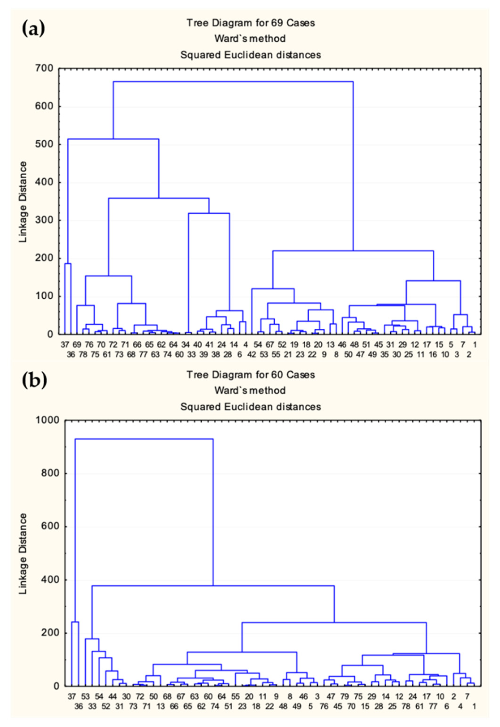
3.5. Hierarchical Cluster Analysis (HCA)

The HCA allowed the classification of the sampling sites into two main groups (1 and 2) by season according to similarities of the physicochemical characteristics of the water samples (Figure 3a,b). In the dry season, group 1 (thirty-one sites) and group 2 (thirty-eight sites) had two subgroups (a,b and c,d, respectively), while in the rainy season, group 1 was formed by two sites, and only group 2 (fifty-eight sites) had two subgroups (a and b). The distance between groups 1 and 2 was minor in the dry season than during the rainy season, suggesting greater similarity. This highlighted that the sites no. 37 and no. 36 formed subgroup 1a and group 1 during the dry and rainy season.

Due to the physicochemical characteristics determining the water quality, this section describes the results according to the WQI values of each sample. Overall, the wastewater injection samples and water from Laguna Verde (sites no. 37 and no. 36, respectively) suggest that the water from these sites differs from drinking water supply sources (mainly during the rainy season). The WQI sites for no. 37 and no. 36 ranged between 3678.3–24,848.9 and 1382.7–31,486.4 during the dry and rainy season, respectively; data showed unsuitable quality water from sites within “Los Azufres” geothermic field. The parameter in common at sites no. 37 and no. 36 during both seasons and with higher level were pH, EC, TDS, acidity, arsenic, and Sb. The waters of both sites have their origin in steam from geothermal groundwater finally, in wells and artificial lagoons, the condensed water loses heat and is injected into the subsoil.

The subgroup 1b (composed of two subgroups) during the dry season included sites of ZIT (no. 60–no. 66, no. 68), TUX (no. 69–no. 78), SPJ (no. 28, no. 33, no. 34, no. 38, no. 39, no. 41), HID (no. 24, no. 14), and ZIN (no. 4, no. 6). Overall, all sites within subgroup 1b showed a WQI value of 19.2–58.6, equivalent to excellent (WQI ≤ 50) and good water quality (WQI = 50–100), except at no. 33, no. 34, and no. 69 (WQI = 132.2, 134.2, and 394.1, respectively; with poor water quality WQI = 100–200 and unsuitable for drinking water WQI ≥ 300). In the dry season, the 2c and 2d subgroups were composed of sites in MAR (no. 45–no. 49), IRI (no. 50–no. 55), HID (no. 9–no. 13, no. 15–no. 23, no. 25), ZIN (no. 1–no. 3, no. 5, no. 7, no. 8), and SPJ (no. 29, no. 30, no. 31, no. 35, no. 42). The WQI of thirty-one sites ranging from 16.8–32.4 from 2c and 2d subgroups showed excellent water quality (mainly sites located in MAR and HID); three sites had index range 62.3–68.9 (good water quality, all sites in ZIN), and one site with WQI = 196.2 (site no. 42 at SPJ with poor water quality).

During the rainy season, subgroup 2a included sites of the IRI (no. 52, no. 53, no. 54) and SPJ (no. 33, no. 30, no. 31, no. 44) community. Site no. 53 of IRI had a WQI = 616.3 which corresponds to water unsuitable for drinking (WQI = >300), while no. 52 (WQI = 87.7) and no. 54 (WQI = 31.3) sites showed values equivalent to good water and excellent water. At SPJ, all sites had WQI ranging from 101.8–404.8, equivalent to poor water quality (sites no. 31 and no. 33), very poor water quality (WQI = 200–300, site no. 30), and unsuitable for drinking water (site no. 44). Finally, in the rainy season, subgroup 2b was composed of all of the sites in ZIN (no. 1–no. 8) and sites from HID (no. 9–no. 15, no. 17, no. 18, no. 20, no. 22–no. 25), MAR (no. 45–no. 49), ZIT (no. 60–no. 68), TUX (no. 70–no. 79), SPJ (no. 28, no. 9), and IRI (no. 50, no. 51, no. 55). All of them are organized into at least two main subgroups. The WQI in subgroup 2b ranged from 21.4–87.8, where thirty-seven sites showed excellent water quality and eleven sites showed good water quality (except site no. 7 of ZIN with WQI = 126.7, equivalent to poor water quality).

The drinking water supply source’s physicochemical characteristics depend on geological characteristics in the study area, and these geological components influence the WQI (although the anthropogenic pollution sources and meteorological events, such as rain and high temperature, also are important). For this reason, the expectation was that the formation of groups coincided with the geographical extension of geological soil type. For example, in the dry season, all TUX and ZIT sites forming subgroup 1b (except site no. 67 from ZIT) were located over igneous rocks of basic and intermediate extrusive type (this also included sites no. 24 and no. 14 from HID, and no. 38–no. 41 of SPJ), while sites no. 4 and no. 6 from ZIN and sites no. 28, no. 33, and 34 in SPJ were located over igneous rocks of acid extrusive type [1,22,40].

Although it is likely that after the wastewater is injected into the subsoil, it could pollute the supply of water for human consumption located downstream (by infiltration), our actual results from HCA indicate that the separation between the group with sites no. 37 and no. 36 and the remaining groups are important, mainly during the rainy season (Figure 3). Furthermore, the physicochemical characteristics of wastewater injection were different from those registered in water samples from sites located near SPJ and ZIN (despite being located near the geothermic field in the limits between the aquifers of Morelia–Queréndaro and Cd. Hidalgo–Tuxpan) in both seasons, despite the high values of different variables in samples of these two populations.

Additional evidence shows that Li⁺, an indicator of geothermic pollution, had high levels only in wastewater injection, which was not found at the other sites [60]. Thus, there is not much information about the pollution of ground wells for public supply near the geothermal energy field, even though pollution was reported with arsenic in surface waters due to drains in pipes and ponds from the geothermic field. Water for injection originates during the elimination of the excess humidity from the steam extracted at the wells within the geothermic field, which is later condensed and cooled in tanks to be injected as water; therefore, its salinity is increased, and it is isotopically richer than the fluids in the deposit [63].

The Laguna Verde (site no. 36) is a water reservoir where wastewaters from the vapor cooling process during electric energy generation are directly discharged. Due to its physicochemical characteristics of water, this hydric system is not used as a source of drinking water supply. This water had low pH levels (2.5) and high levels of TDS, turbidity, color, COD, SO₄²⁻, Fe, Al, arsenic, and Mn. Potential situations involving pollution due to improper management of these wastewaters have been reported in the case of leaks in pipes or direct discharges from this activity [23,45,55]. Based on cluster analysis, the similarity in the physicochemical characteristics of wastewater injection and water located in Laguna Verde that generate an independent cluster are evident; however, there is no statistical evidence of a direct influence on the chemical composition of the nearest sites for water supply, especially those in SPJ and ZIN.

On the other hand, the Laguna Larga (site located in SPJ), a natural surface body of water, had a very low pH (near 3), and high turbidity, color, Al, arsenic, and Mn. The water from Laguna Larga is used as a source of water supply for human consumption and other productive activities with the permanent contact of the surrounding population. Therefore, it is necessary to have control and continuous monitoring of its quality [23,55,56,57,58]. It is highlighted that during the dry season, the group formed by water samples from Laguna Larga (sites no. 33 and no. 34) was more closely related with the subgroup 1b, which was composed of sites in SPJ (sites no. 28 and no. 38–no. 41), HID (sites no. 14, no. 24), and ZIN (sites no. 4, no. 6). The likelihood is that the small physical distance between those sites and Laguna Larga might be why they constitute related groups and why there might be a possible influence on the characteristics of their waters. All sites were located inside an area of high geothermal activity, which is the likely cause of such similarities.

Finally, the actual data are insufficient evidence of the influence between the injection water and the Laguna Verde water on the composition of the water supply sources for human consumption in the surrounding area. This suggests that the regions of water supply sources for consumption are probably not contaminated by sewage from the “Los Azufres” geothermal field.

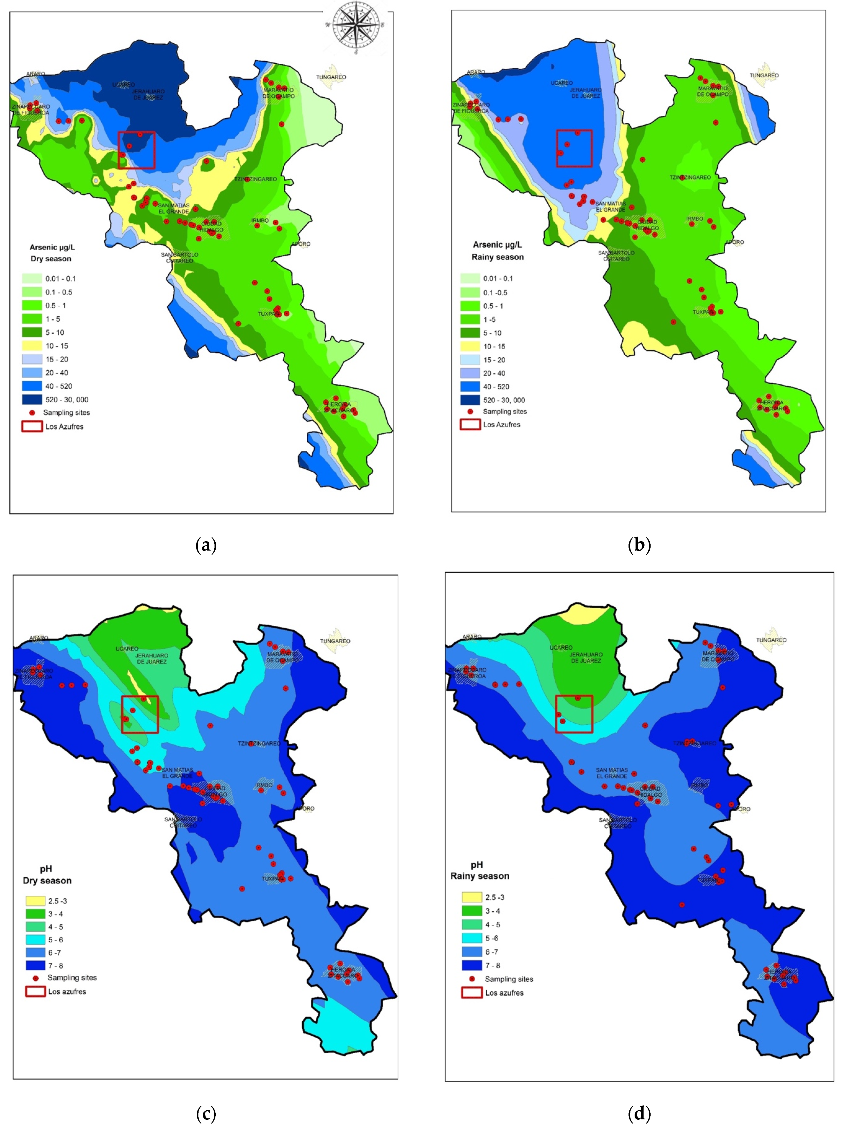
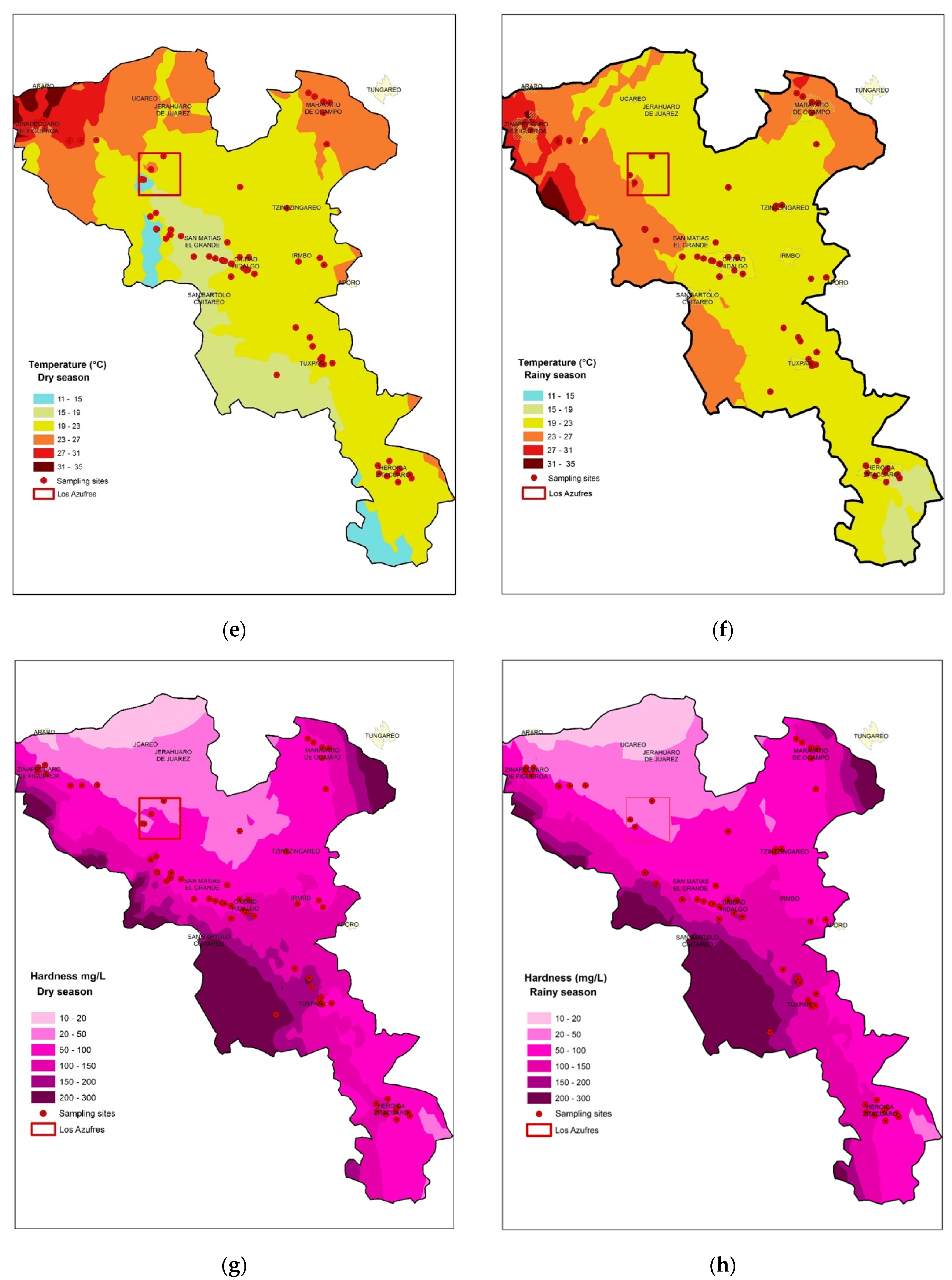
3.6. Description of the Spatial Distribution of Parameters by GIS

Figure 4 shows the main sites of water sampling for the dry and rainy seasons and the spatial distribution of parameters using GIS data and kriging spatial interpolation. This analysis technique allows estimation of the potential concentrations of the considered variables in this study in different places with possible negative effects on human health [12,60,62]. Overall, the results from GIS highlight some communities with low populations without data from sampling and analysis sites. Many small communities inside this area are not mentioned in the text due to the higher number but low population.

During the dry season, one part of the area of operation of the geothermic field and its surroundings shows zones with higher concentrations of arsenic (Figure 4a). Some of the communities in the surroundings, Jeráhuaro and Ucareo (both located north of “Los Azufres”), Araró (at the north of ZIN), and the surroundings of ZIN, are located in areas where there could be high arsenic concentrations (520–30,000 µg/L). Some reports in the literature indicate that the community of Araró possesses water with high concentrations of arsenic and F⁻, which is partly due to the geothermic activity [60,62,64]. The Tzinzingareo community in dry season shows pH between 1–5, and 5–15 µg/L of arsenic. Finally, small communities in the southwestern TUX and ZIT municipalities could show high concentrations of arsenic in this season [65,66].

On the other hand, during the rainy season (Figure 4b), areas with arsenic concentrations between 40–520 µg/L were located at the central part of the geothermal field and its surroundings. It is probable that some sites in ZIN and SPJ also show concentrations in this range. An even larger number of sites in SPJ have concentrations between 15–20 µg/L. The likelihood is that the presence of rain has two effects on the possible distribution of arsenic in water; in one way, it dilutes its concentrations by the great volume of rain. On the other hand, it creates the extent of such areas with lower to higher concentrations of arsenic, due to lixiviation to downstream by water rain. However, in both seasons, the projected areas show higher concentrations than the limits established by international regulations for water for human consumption. The geothermic field is located precisely in these areas, suggesting the possible influence of its activity, along with geological and geothermal conditions from the surroundings, on the high arsenic levels in this area and the drinking water supply sites. In this sense, the areas with high concentrations of arsenic in both seasons are located mainly above geologic formations of acid extrusive igneous rocks (Figure 1). Zones with concentrations between 1–5 and 5–10 µg/L of arsenic, both during the dry and the rainy season, included practically all of the sites in MAR, HID, TUX, IRI, and ZIT.

For pH, during the dry and rainy seasons (Figure 4c,d, respectively), the water within the area of operation of the geothermic field was found mainly to be between acidic to slightly acidic pH (3–4 and 5–6, respectively), which is outside the limits established by international and national regulations, respectively [40,42]. The geologic composition of the region probably influences the pH levels of water. During both seasons, ZIN, HID, MAR, TUX, IRI, and ZIT had pH levels of 6–7 (slightly acid to neutral) and pH 7–8 (neutral to slightly alkaline), respectively, with specific variations in each case (except SPJ during the dry season, with pH 5–6). In places such as HID, TUX, and ZIT, the geologic composition includes extrusive basic igneous rocks, which could explain part of the variation in pH between seasons. The forecast for Jeráhuaro and Ucareo is pH 3–4 and pH 4–5 during the dry season and pH 3–4 during the rainy season. In the dry season, communities such as Araró show pH of 6–7, and during the rainy season, pH of 5–6. Cuitareo, Aporo, and Tzinzingareo in both seasons have pH levels ranged 6–8.

In both seasons, all sites of ZIN were in areas with the highest levels of temperature (27–31 °C) (Figure 4e,f, respectively). For both seasons, municipalities such as HID, IRI, TUX, and ZIT were in areas with a range of 19–23° C, and MAR had temperatures of 23–27 °C. During the dry season, the SPJ and HID sites were in zones with temperatures in the range of 15–19 °C. It has been reported that at temperatures >25 °C, the dissolution of some elements, such as arsenic, from subsoil is favored [58]. The conditions at Araró stood out by their elevated temperature (27–31 °C and 31–35 °C); Ucareo, Aporo, and Jeráhuaro ranged between 19–23 °C and 23–27 °C; Cuitareo showed temperatures of 15–19 °C; and Tzinzingareo had a moderate temperature (19–23 °C) during the dry season. Overall, a big ZIN and SPJ communities area showed elevated temperatures ranging from 23–27 °C and 31–35 °C during the rainy season. In the rainy season, Araró mainly showed temperatures between 23–37 °C, Ucareo, Jeráhuaro, Tzinzingareo, and Aporo had temperatures of 19–23 °C, and Cuitareo showed a range between 19–27 °C.

The variation in hardness concentrations in the dry and rainy seasons (Figure 4g,h, respectively) showed a similar distribution. Most of the sampling sites were in areas with hardness levels between 20–50 and 50–100 mg/L of CaCO₃. This included the operational area of the geothermic field. In both seasons, places such as Araró, Ucareo, and Jeráhuaro might have levels between 10–20 and 20–50 mg/L of CaCO₃, while Cuitareo might attain levels of 200–300 mg/L for CaCO₃, and Aporo between 20–50 and 50–100 mg/L during the dry and rainy season, respectively. Tzinzingareo in both seasons had a level of 50–100 mg/mL.

The results from this section allow us to stood up that there is a potential risk of exposure to various pollutants in the water supply sources for the populations of the main communities (209,142 inhabitants of ZIN, SPJ, HID, MAR, IRI, TUX, and ZIT), and in communities with minority populations. Communities such as Araró, Ucareo, Jeráhuaro, Cuitareo, Aporo, and Tzinzingareo have at least 16,383 inhabitants, most of the population is from farms and small settlements distributed in the study area.

However, the projections used by GIS and the kriging interpolation model have limitations for a larger scale. The study area has the equivalent of 1600 km². In comparison, the state of Michoacán has a study area of 58,599 km². In addition, considering the territorial extent of the western region of Mexico (states of Nayarit, Jalisco, and Colima, with a total of approximately 171,000 km²), the territorial differences within the study area become more noticeable. Therefore, the field information obtained regarding water quality is a limitation to propose interpolations at the state level and in the western region of the country. Nevertheless, the reported data are relevant to lay the basis for broader research and to select a larger number of sampling sites for water for human supply within several annual cycles.

3.7. Health Risk Assessment

The noncancer risk by dermal and oral ingestion was calculated as HQ and HI in adults, children, and infants (

Table 6. Calculated hazard quotients (HQ) due to oral and dermal exposure of metals in water.

	Rainy Season						Dry Season
	HQ Oral			HQ Dermal			HQ Oral			HQ Dermal
Parameter	Adults	Children	Infants	Adults	Children	Infants	Adults	Children	Infants	Adults	Children	Infants
Ba	5.2 × 10−3	5.2 × 10−3	1.6 × 10−2	3.0 × 10−4	4.1 × 10−4	5.9 × 10−4	3.8 × 10−3	3.8 × 10−3	1.1 × 10−2	2.2 × 10−4	3.0 × 10−4	4.3 × 10−4
Cr	3.6 × 10−2	3.6 × 10−2	1.1 ×10−1	8.3 × 10−2	1.1 × 10−1	1.6 × 10−1	4.6 × 10−3	4.6 × 10−3	1.4 × 10−2	1.0 × 10−2	1.4 × 10−2	2.1 × 10−2
Cd	1.3 × 10−3	1.3 × 10−3	3.9 × 10−3	1.5 × 10−3	2.0 × 10−3	2.8 × 10−3	1.0 × 10−3	1.0 × 10−3	3.1 × 10−3	1.2 × 10−3	1.6 × 10−3	2.3 × 10−3
Pb	2.6 × 10−3	2.6 × 10−3	7.8 × 10−3	9.9 × 10−5	1.4 × 10−4	1.9 × 10−4	3.9 × 10−3	3.9 × 10−3	1.2 × 10−2	1.5 × 10−4	2.0 × 10−4	2.9 × 10−4
As	5.7 × 100	5.7 × 100	1.7 × 10+1	1.6 × 10−1	2.2 × 10−1	3.0 × 10−1	1.9 × 10−1	1.9 × 10−1	5.7 × 10−1	5.3 × 10−3	7.3 × 10−3	1.0 × 10−2
Mn	8.2 × 10−3	8.1 × 10−3	2.4 × 10−2	2.3 × 10−3	3.2 × 10−3	4.4 × 10−3	1.4 × 10−2	1.4 × 10−2	4.3 × 10−2	4.1 × 10−3	5.6 × 10−3	8.1 × 10−3
Ni	9.4 × 10−4	9.3 × 10−4	2.8 × 10−3	3.9 × 10−5	5.4 × 10−5	7.5 × 10−5	2.7 × 10−4	2.7 × 10−4	8.0 × 10−4	1.1 × 10−5	1.5 × 10−5	2.2 × 10−5
∑HI	5.8 × 100	5.8 × 100	1.7 × 10+1	2.5 × 10−1	3.4 × 10−1	4.7 × 10−1	2.2 × 10−1	2.2 × 10−1	6.6 × 10−1	2.1 × 10−2	2.3 × 10−2	4.2 × 10−2

). The HI > 1 for the three groups is only for oral exposure and in the rainy season, and the rest is < 1 for the three groups is for oral in the dry season, and for dermal in the rainy season.

The hazard quotient values associated with arsenic for oral exposition for all classified groups were higher than the reference (>1) in the rainy season, in contrast to the dry season. However, it cannot be concluded that potential noncarcinogenic risks are nonexistent in the season, as exposure to arsenic through food and inhalation may also pose a risk.

Runoff processes can explain the high levels of arsenic in the rainy season from geothermal fields. In addition, symptoms of chronic arsenic poisoning, such as skin lesions and high arsenic concentrations in hair and nails, have been reported in geothermal fields [67].

Chronic exposure to high levels of arsenic causes a wide variety of serious human health problems, including changes in dermal pigmentation, hyperkeratosis and ulceration, various types of cancer (skin, bladder, lung, kidney, and other organs), respiratory, pulmonary, hematological, hepatic, renal, developmental, reproductive, immunological, genotoxic, and mutagenetic effects [68].

Table 7. Calculated incremental lifetime cancer risk (ILCR) values due to oral and dermal exposure of metals in water.

	Rainy Season						Dry Season
	ILCR Oral			ILCR Dermal			ILCR Oral			ILCR Dermal
Parameter	Adults	Children	Infants	Adults	Children	Infants	Adults	Children	Infants	Adults	Children	Infants
Cr	4.6 × 10−5	4.6 × 10−5	1.4 × 10−4	5.2 × 10−7	7.2 × 10−7	9.9 × 10−7	5.8 × 10−6	5.7 × 10−6	1.7 × 10−5	6.5 × 10−8	9.0 × 10−8	1.3 × 10−7
Cd	9.8 × 10−6	9.8 × 10−6	2.9 × 10−5	1.1 × 10−7	1.5 × 10−7	2.1 × 10−7	7.8 × 10−6	7.8 × 10−6	2.3 × 10−5	8.9 × 10−8	1.2 × 10−7	1.8 × 10−7
Pb	3.1 × 10−8	3.1 × 10−8	9.3 × 10−8	3.5 × 10−10	4.8 × 10−10	6.7 × 10−10	4.7 × 10−8	4.6 × 10−8	1.4 × 10−7	5.3 × 10−10	7.3 × 10−10	1.0 × 10−9
As	2.6 × 10−3	2.6 × 10−3	7.7 × 10−3	2.9 × 10−5	4.0 × 10−5	5.6 × 10−5	8.6 × 10−5	8.6 × 10−5	2.6 × 10−4	9.8 × 10−7	1.3 × 10−6	1.9 × 10−6
Ni	1.7 × 10−5	1.7 × 10−5	5.1 × 10−5	1.9 × 10−7	2.7 × 10−7	3.7 × 10−7	4.9 × 10−6	4.9 × 10−6	1.5 × 10−5	5.5 × 10−8	7.6 × 10−8	1.1 × 10−7
∑ILCR	2.7 × 10−3	2.6 × 10−3	7.9 × 10−3	3.0 × 10−5	4.1 × 10−5	5.7 × 10−5	1.0 × 10−4	1.0 × 10−4	3.1 × 10−4	1.2 × 10−6	1.6 × 10−6	2.4 × 10−6

shows the possibility of exposed subjects developing cancer from lifetime exposure to metals. Although infants, children, and adults are at a higher risk (1 × 10⁻³) through oral ingestion, especially during the rainy season when concentrations of arsenic increase, dermal contact does not constitute a threat below the range of 1 × 10⁻⁶ to 1 × 10⁻⁴ [69,70]. Arsenic has the highest chance of cancer risks (1×10⁻³), and lead has the lowest probability of cancer risk (1 × 10⁻⁸). These results present a cancer risk from the contaminants to residents through the cumulative ingestion in the region’s drinking water. It has been reported that ingestion of arsenic in drinking water in early childhood might increase liver cancer mortality. In addition, arsenic in drinking water is established to be a major cause of adult cancer in exposed populations [71]. However, to our knowledge, there are no reports in the region to assess the impact of groundwater arsenic on people’s health.

4. Conclusions

Most parameters for water quality for human consumption were evaluated within limits established by international and national regulations. In some cases, they were outside those limits, such as low pH levels, turbidity, color, Fe, Al, Mn, and arsenic. ZIN, HID, and SPJ stood out for having more sites and parameters with levels outside limits established, mainly of arsenic. The calculated WQI suggests that, mainly in the dry season and for each municipality, the water had a classification of “excellent water” and “good water quality”, and, only in the rainy season, the WQI of SPJ and IRI showed “poor water quality”.

The PCA and HCA suggested that pollution of geologic and geothermal origin (the type of rock, and rock-groundwater interactions) contributes to increasing the levels of most of the parameters analyzed in this study. In addition, the rain is a seasonal factor that elevates concentrations of some chemical substances and influences the increase in several parameters, possibly due to processes such as lixiviation, for a larger amount of water from pluvial precipitations.

The GIS led to the prediction and continuous characterization of the concentrations of each study variable.

For three target groups, the noncancer risk level exceeded the recommended criteria in the rainy season, suggesting that the presence of metals represents a threat to the health of adults, children, and infants. The carcinogenic risk of water consumption based on ingestion exposure is high; therefore, residents in this study area may be at increased health risk, and authorities should pay close attention to this area. Furthermore, based on exposure assessments, children may be at increased risk for carcinogens and noncarcinogens mainly through ingestion of Arsenic. The information generated by the present work is a starting point for a better understanding of possible relationships between the water supply quality for human consumption and human health effects in the study regions. Such understanding could be attained when results such as those presented here are matched to those derived from epidemiologic studies regarding the number of disease cases in different sectors of the human populations of Cuitzeo and the eastern Michoacán regions.

References

1. WHO. Protecting Groundwater for Health: Managing the Quality of Drinking-Water Sources; Schmoll, O., Howard, G., Chilton, J., Chorus, I., Eds.; IWA Publishing: London, UK, 2006; ISBN 9781843390794. [Google Scholar]
2. Altenburger, R.; Brack, W.; Burgess, R.M.; Busch, W.; Escher, B.I.; Focks, A.; Mark Hewitt, L.; Jacobsen, B.N.; de Alda, M.L.; Ait-Aissa, S.; et al. Future water quality monitoring: Improving the balance between exposure and toxicity assessments of real-world pollutant mixtures. Environ. Sci. Eur. 2019, 31, 1–17. [Google Scholar] [CrossRef] [Green Version]
3. WHO. Arsenic in Drinking-Water: Background Document for Development of WHO Guidelines for Drinking-Water Quality; World Health Organization: Geneva, Switzerland, 2003; Volume WHO/SDE/WS. [Google Scholar]
4. WHO. Fluoride in Drinking-Water: Background Document for Development of WHO Guidelines for Drinking-Water Quality; World Health Organization: Geneva, Switzerland, 2004. [Google Scholar]
5. WHO. Selenium in Drinking-Water: Background Document for Development of WHO Guidelines for Drinking-Water Quality; World Health Organization: Geneva, Switzerland, 2003. [Google Scholar]
6. Reilly, R.; Spalding, S.; Walsh, B.; Wainer, J.; Pickens, S.; Royster, M.; Villanacci, J.; Little, B.B. Chronic environmental and occupational lead exposure and kidney function among African Americans: Dallas lead project II. Int. J. Environ. Res. Public Health 2018, 15, 2875. [Google Scholar] [CrossRef] [Green Version]
7. Kulathunga, M.R.D.L.; Ayanka Wijayawardena, M.A.; Naidu, R.; Wijeratne, A.W. Chronic kidney disease of unknown aetiology in Sri Lanka and the exposure to environmental chemicals: A review of literature. Environ. Geochem. Health 2019, 41, 2329–2338. [Google Scholar] [CrossRef]
8. Kumar, A.; Subrahmanyam, G.; Mondal, R.; Shabnam, A.A.; Jigyasu, D.K.; Malyan, S.K.; Kishor-fagodiya, R.; Khan, S.A.; Kumar, A.; Yu, Z. Bio-remediation approaches for alleviation of cadmium contamination in natural resources. Chemosphere 2020, 268, 128855. [Google Scholar] [CrossRef]
9. Kumar, A.; Pinto, M.C.; Candeias, C.; Dinis, P.A. Baseline maps of potentially toxic elements in the soils of Garhwal Himalayas, India: Assessment of their eco-environmental and human health risks. Land Degrad. Dev. 2021. [Google Scholar] [CrossRef]
10. Kumar, A.; Kumar, A.; Chaturvedi, A.K. Lead toxicity: Health hazards, influence on food chain, and sustainable remediation approaches. Int. J. Environ. Res. Public Health 2020, 17, 2179. [Google Scholar] [CrossRef] [Green Version]
11. Fevrier-Paul, A.; Soyibo, A.K.; Mitchell, S.; Voutchkov, M. Role of toxic elements in chronic kidney disease. J. Health Pollut. 2018, 8, 181202. [Google Scholar] [CrossRef] [PubMed]
12. Şener, Ş.; Şener, E.; Davraz, A. Evaluation of water quality using water quality index (WQI) method and GIS in Aksu River (SW-Turkey). Sci. Total Environ. 2017, 584–585, 131–144. [Google Scholar] [CrossRef]
13. Kawo, N.S.; Karuppannan, S. Groundwater quality assessment using water quality index and GIS technique in Modjo River Basin, central Ethiopia. J. Afr. Earth Sci. 2018, 147, 300–311. [Google Scholar] [CrossRef]
14. Jha, M.K.; Shekhar, A.; Jenifer, M.A. Assessing groundwater quality for drinking water supply using hybrid fuzzy-GIS-based water quality index. Water Res. 2020, 179, 115867. [Google Scholar] [CrossRef]
15. Nnorom, I.C.; Ewuzie, U.; Eze, S.O. Multivariate statistical approach and water quality assessment of natural springs and other drinking water sources in Southeastern Nigeria. Heliyon 2019, 5, e01123. [Google Scholar] [CrossRef] [Green Version]
16. Moldovan, A.; Maria-Alexandra Hoaghia, E.K.; Mirea, I.C.; Kenesz, M.; Răzvan Adrian Arghir, A.P.; Levei, E.A.; Moldovan, O.T. Quality and health risk assessment associated with water consumption—A case study on Karstic springs. Water 2020, 12, 3510. [Google Scholar] [CrossRef]
17. Hussain, S.; Habib-ur-Rehman, M.; Khanam, T.; Sheer, A.; Kebin, Z.; Jianjun, Y. Health risk assessment of different heavy metals dissolved in drinking water. Int. J. Environ. Res. Public Health 2019, 16, 1737. [Google Scholar] [CrossRef] [Green Version]
18. Jayasumana, C.; Paranagama, P.A.; Amarasinghe, M.D.; Wijewardane, K.M.R.C.; Dahanayake, K.S.; Fonseka, S.I.; Rajakaruna, K.D.L.M.P.; Mahamithawa, A.M.P.; Samarasinghe, U.D.; Senanayake, V.K. Possible link of chronic arsenic toxicity with Chronic Kidney Disease of unknown etiology in Sri Lanka. J. Nat. Sci. Res. 2013, 3, 64–73. [Google Scholar]
19. Qafoku, N.P.; Lawter, A.R.; Bacon, D.H.; Zheng, L.; Kyle, J.; Brown, C.F. Review of the impacts of leaking CO2 gas and brine on groundwater quality. Earth Sci. Rev. 2017, 169, 69–84. [Google Scholar] [CrossRef] [Green Version]
20. Morfin-Otero, R.; Garza-Gonzalez, E.; Garcia, G.G.; Perez-Gomez, H.R.; Aguirre-Diaz, S.A.; Gonzalez-Diaz, E.; Esparza-Ahumada, S.; Fernandez-Ramirez, A.; Cardenas-Lara, F.; Martinez-Melendez, A.; et al. Clostridium difficile infection in patients with chronic kidney disease in Mexico. Clin. Nephrol. 2018, 90, 350–356. [Google Scholar] [CrossRef]
21. Villalobos-Castañeda, B.; Cortés-Martínez, R.; Segovia, N.; Buenrostro-Delgado, O.; Morton-Bermea, O.; Alfaro-Cuevas-Villanueva, R. Distribution and enrichment of trace metals and arsenic at the upper layer of sediments from Lerma River in La Piedad, Mexico: Case history. Environ. Earth Sci. 2016, 75, 1490. [Google Scholar] [CrossRef]
22. INEGI. Red Hidrográfica Escala 1:50000 Edición 2.0; Dirección General de Geografía y Medio Ambiente: Aguascalientes, México, 2010.
23. Gutiérrez Negrín, L.C.A.; Lippmann, M.J. Mexico: Thirty-three years of production in the Los Azufres geothermal field. Geotherm. Power Gener. Dev. Innov. 2016, 717–742. [Google Scholar] [CrossRef]
24. American Public Health Association; American Water Works Association; Water Environmental Federation. Standard Methods for the Examination of Water and Wastewater, 23rd ed.; Baird, B.R., Eaton, D.A., Rice, E.W., Eds.; American Public Health Association: Washington, DC, USA, 2017. [Google Scholar]
25. Kowalkowski, T.; Zbytniewski, R.; Szpejna, J.; Buszewski, B. Application of chemometrics in river water classification. Water Res. 2006, 40, 744–752. [Google Scholar] [CrossRef]
26. Lattin, J.M.; Carroll, J.D.; Green, P. Analyzing Multivariate Data, 2nd ed.; Brooks/Cole: New York, NY, USA, 2003. [Google Scholar]
27. Karroum, L.A.; El Baghdadi, M.; Barakat, A.; Meddah, R.; Aadraoui, M.; Oumenskou, H.; Ennaji, W. Assessment of surface water quality using multivariate statistical techniques: EL Abid River, Middle Atlas, Morocco as a case study. Desalin. Water Treat. 2019, 143, 118–125. [Google Scholar] [CrossRef]
28. Sharma, S. Applied Multivariate Techniques, 2nd ed.; John Wiley and Sons: New York, NY, USA, 1996. [Google Scholar]
29. Li, J.; Heap, A.D. Spatial interpolation methods applied in the environmental sciences: A review. Environ. Model. Softw. 2014, 53, 173–189. [Google Scholar] [CrossRef]
30. De Smith, M.J.; Goodchild, M.F.; Longley, P. Geospatial Analysis: A Comprehensive Guide to Principles, Techniques and Software Tools, 2nd ed.; Troubador Publishing Ltd: Leicester, UK, 2007. [Google Scholar]
31. Garcia-Papani, F.; Leiva, V.; Ruggeri, F.; Uribe-Opazo, M.A. Kriging with external drift in a Birnbaum–Saunders geostatistical model. Stoch. Environ. Res. Risk Assess. 2018, 32, 1517–1530. [Google Scholar] [CrossRef]
32. US Environmental Protection Agency. Exposure Factors Handbook: 2011 Edition; PA: Washington, DC, USA, 2011; ISBN EPA/600/R-090/052F. [Google Scholar]
33. Agency for Toxic Substances and Disease Registry. Public Health Assessment Guidance Manual (Update); Agency for Toxic Substances and Disease Registry: Atlanta, GA, USA, 2005.
34. Mohammadi, A.A.; Zarei, A.; Majidi, S.; Ghaderpoury, A.; Hashempour, Y.; Saghi, M.H.; Alinejad, A.; Yousefi, M.; Hosseingholizadeh, N.; Ghaderpoori, M. Carcinogenic and non-carcinogenic health risk assessment of heavy metals in drinking water of Khorramabad, Iran. MethodsX 2019, 6, 1642–1651. [Google Scholar] [CrossRef]
35. US EPA Risk Assessment Guidance for Superfund Volume I: Human Health Evaluation Manual (Part F, Supplemental Guidance for Inhalation Risk Assessment); EPA: Washington, DC, USA, 2009; pp. 1–68.
36. Tripathee, L.; Kang, S.; Sharma, C.M.; Rupakheti, D.; Paudyal, R.; Huang, J.; Sillanpää, M. Preliminary Health risk assessment of potentially toxic metals in surface water of the Himalayan rivers, Nepal. Bull. Environ. Contam. Toxicol. 2016, 97, 855–862. [Google Scholar] [CrossRef]
37. Li, R.; Liu, Y.K.W.; Enmin, C.J. Potential health risk assessment through ingestion and dermal contact arsenic-contaminated groundwater in Jianghan Plain, China. Environ. Geochem. Health 2018, 40, 1585–1599. [Google Scholar] [CrossRef]
38. OEHHA. California Office of Environmental Health Hazard Assessment (OEHHA). Technical Support Document for Cancer Potency Factors 2009, Appendix A: Hot Spots Unit Risk and Cancer Potency Values; OEHHA: Sacramento, CA, USA, 2019.
39. U.S. Environmental Protection Agency. Integrated Risk Information System; EPA: Washington, DC, USA, 1987.
40. WHO. Guidelines for Drinking-Water Quality: Incorporating 1st and 2nd Addenda Recommendations, 3rd ed.; World Health Organization: Geneva, Switzerland, 2008; Volume 1. [Google Scholar]
41. Secretaría de Salud. Bienes y Servicios. Agua purificada envasada. Especificaciones Sanitarias. Secretaría de Salud. NOM-041-SSA1; Diario Oficial de la Federación: Mexico City, Mexico, 1993.
42. Secretaría de Salud. Salud ambiental, Agua para Uso y Consumo Humano. Límites Permisibles de Calidad y Tratamientos a que debe Someterse el Agua para su Potabilización. Secretaría de Salud. NOM-127-SSA1; Diario Oficial de la Federación: Mexico City, Mexico, 1994.
43. Panduro-Rivera, M.G.; Hernández-Mena, L.; López-López, A.; Murillo-Tovar, M.A.; Díaz-Torres, J.J.; del Real-Olvera, J. Evaluación de la calidad del agua ante la enfermedad renal crónica en la Zona Oriente de Michoacán, México. Tlamati 2014, 5, 22–32. [Google Scholar]
44. Zhao, M.M.; Chen, Y.P.; Xue, L.G.; Fan, T.T.; Emaneghemi, B. Greater health risk in wet season than in dry season in the Yellow River of the Lanzhou region. Sci. Total Environ. 2018, 644, 873–883. [Google Scholar] [CrossRef] [PubMed]
45. Idoko, O.M.; Ologunorisa, T.E.; Okoya, A.A. Temporal variability of heavy metals concentration in rural groundwater of Benue State, Middle Belt, Nigeria. J. Sustain. Dev. 2012, 5, 2. [Google Scholar] [CrossRef] [Green Version]
46. Verma, S.P.; Pandarinath, K.; Bhutani, R.; Dash, J.K. Mineralogical, chemical, and Sr-Nd isotopic effects of hydrothermal alteration of near-surface rhyolite in the Los Azufres geothermal field, Mexico. Lithos 2018, 322, 347–361. [Google Scholar] [CrossRef]
47. Pérez-Espinosa, R.; Pandarinath, K.; Hernández-Campos, F.J. CCWater—A computer program for chemical classification of geothermal waters. Geosci. J. 2019, 23, 621–635. [Google Scholar] [CrossRef]
48. Viswanath, N.C.; Kumar, P.G.D.; Ammad, K.K.; Kumari, E.R.U. Ground water quality and multivariate statistical methods. Environ. Process. 2015, 2, 347–360. [Google Scholar] [CrossRef]
49. Hem, D. Study and Interpretation of the Chemical Characteristics of Natural Water; Geological Survey USA: Alexandria, VA, USA, 1985.
50. CONAGUA. Actualización de la Disponibilidad Media Anual de Agua en el Acuífero Maravatío—Contepec—Epitacio Huerta (1601), Estado de Michoacán; Diario Oficial de la Federación: Mexico City, Mexico, 2020.
51. CONAGUA. Actualización de la Disponibilidad Media Anual de Agua en el Acuífero Morelia—Queréndaro (1602), Estado de Michoacán; Diario Oficial de la Federación: Mexico City, Mexico, 2020.
52. CONAGUA. Actualización de la Disponibilidad Media Anual de Agua en el Acuífero Ciudad Hidalgo—Tuxpan (1610), Estado de Michoacán; Diario Oficial de la Federación: Mexico City, Mexico, 2020.
53. CONAGUA. Actualización de la Disponibilidad Media Anual de Agua en el Acuífero Huetamo (1612), Estado de Michoacán; Diario Oficial de la Federación: Mexico City, Mexico, 2020.
54. Fitts, C.R. Groundwater Science; Academic Press: Cambridge, MA, USA, 2012. [Google Scholar]
55. Karthikeyan, S.; Palaniappan, P.R.; Sabhanayakam, S. Influence of pH and water hardness upon nickel accumulation in edible fish Cirrhinus mrigala. J. Environ. Biol. 2007, 28, 489–492. [Google Scholar] [PubMed]
56. Aissaoui, A.; Sadoudi-Ali Ahmed, D.; Cherchar, N.; Gherib, A. Assessment and biomonitoring of aquatic pollution by heavy metals (Cd, Cr, Cu, Pb and Zn) in Hammam Grouz Dam of Mila (Algeria). Int. J. Environ. Stud. 2017, 74, 428–442. [Google Scholar] [CrossRef]
57. Pérez-Denicia, E.; Fernández-Luqueño, F.; Vilariño-Ayala, D.; Manuel Montaño-Zetina, L.; Alfonso Maldonado-López, L. Renewable energy sources for electricity generation in Mexico: A review. Renew. Sustain. Energy Rev. 2017, 78, 597–613. [Google Scholar] [CrossRef]
58. Alarcón-Herrera, M.T.; Bundschuh, J.; Nath, B.; Nicolli, H.B.; Gutierrez, M.; Reyes-Gomez, V.M.; Nuñez, D.; Martín-Dominguez, I.R.; Sracek, O. Co-occurrence of arsenic and fluoride in groundwater of semi-arid regions in Latin America: Genesis, mobility and remediation. J. Hazard. Mater. 2013, 262, 960–969. [Google Scholar] [CrossRef]
59. López, D.L.; Bundschuh, J.; Birkle, P.; Armienta, M.A.; Cumbal, L.; Sracek, O.; Cornejo, L.; Ormachea, M. Arsenic in volcanic geothermal fluids of Latin America. Sci. Total Environ. 2012, 429, 57–75. [Google Scholar] [CrossRef]
60. Aksoy, N.; Şimşek, C.; Gunduz, O. Groundwater contamination mechanism in a geothermal field: A case study of Balcova, Turkey. J. Contam. Hydrol. 2009, 103, 13–28. [Google Scholar] [CrossRef]
61. Bonte, M.; van Breukelen, B.M.; Stuyfzand, P.J. Temperature-induced impacts on groundwater quality and arsenic mobility in anoxic aquifer sediments used for both drinking water and shallow geothermal energy production. Water Res. 2013, 47, 5088–5100. [Google Scholar] [CrossRef]
62. Sathe, S.S.; Mahanta, C. Groundwater flow and arsenic contamination transport modeling for a multi aquifer terrain: Assessment and mitigation strategies. J. Environ. Manag. 2019, 231, 166–181. [Google Scholar] [CrossRef]
63. Armienta, M.A.; Rodríguez, R.; Ceniceros, N.; Cruz, O.; Aguayo, A.; Morales, P.; Cienfuegos, E. Groundwater quality and geothermal energy. The case of Cerro Prieto Geothermal Field, México. Renew. Energy 2014, 63, 236–254. [Google Scholar] [CrossRef]
64. Mendoza, L.A.; Del Razo, L.M.; Barbier, O.; Saldaña, M.C.M.; González, F.J.A.; Juárez, F.J.; Sánchez, J.L.R. Potable water pollution with heavy metals, arsenic, and fluorides and chronic kidney disease in infant population of aguascalientes. In Water Resources in Mexico: Scarcity, Degradation, Stress, Conflicts, Management, and Polic; Spring, Ú.O., Ed.; Springer: Berlin/Heidelberg, Germany, 2011; ISBN 9783642054327. [Google Scholar]
65. Reyes, R.M.B.; Gómez, V.M.A.; Mendoza, A.; Reyes, L. Variación de la composición del vapor en pozos del campo geotérmico de Los Azufres, México, por efecto de la reinyección. Geotermia 2012, 25, 3–9. [Google Scholar]
66. Birkle, P.; Merkel, B. Environmental impact by spill of geothermal fluids at the geothermal field of Los Azufres, Michoacán, México. Water Air Soil Pollut. 2000, 124, 371–410. [Google Scholar] [CrossRef]
67. Welch, A.H.; Stollenwerk, K. Arsenic in Groundwater Geochemistry and Occurrence; Kluwer Academic Publishers: Dordrecht, The Netherlands, 2003. [Google Scholar]
68. Hong, Y.S.; Song, K.H.; Chung, J.Y. Health effects of chronic arsenic exposure. J. Prev. Med. Public Health 2014, 47, 245–252. [Google Scholar] [CrossRef] [Green Version]
69. Robson, M.G.; Toscano, W.A. Risk Assessment for Environmental Health; John Wiley & Sons, Inc.: San Francisco, CA, USA, 2007; ISBN 9780787983192. [Google Scholar]
70. Agency for Toxic Substances and Disease Registry. Guidance Manual for the Assessment of Joint Toxic Action of Chemical Mixtures; Agency for Toxic Substances and Disease Registry: Atlanta, GA, USA, 2004.
71. Liaw, J.; Marshall, G.; Yuan, Y.; Ferreccio, C.; Steinmaus, C.; Smith, A.H. Increased childhood liver cancer mortality and arsenic in drinking water in Northern Chile. Cancer Epidemiol. Biomark. Prev. 2008, 17, 1982–1987. [Google Scholar] [CrossRef] [PubMed] [Green Version]
Figure 1. Map of the geographic extension of the municipalities, geology of the regions under study, and extension of the aquifers where sampling sites were located. The geothermic field is shown in red.
Water 13 02196 g001
Figure 2. Quality parameters of drinking water supply sources for humans in the regions of study that stood out due to higher levels concerning the permissible limits defined by WHO, NOM-040, and NOM-127: (a) pH; (b) turbidity; (c) color; (d) iron; (e) aluminum; (f) arsenic. Green dots (): rainy season, yellow dots (): dry season. Vertical lines on the secondary x-axis represent the distribution of each municipality.
Water 13 02196 g002
Figure 3. Dendrograms generated by hierarchical cluster analysis show the groups formed by the different sampling sites during (a) dry and (b) rainy seasons—groups 1 and 2, subgroups a, b, c, and d. There is no statistical evidence of a direct influence of the “Los Azufres” geothermic field on the chemical composition of the nearest sites for water supply, especially those in SPJ and ZIN.
Water 13 02196 g003
Figure 4. Spatial distribution maps generated by GIS through the kriging spatial interpolation method for both seasons. Here, the possible concentrations or levels of different parameters are observed: Arsenic (a,b); pH (c,d); temperature (e,f); hardness (g,h). The geothermic field is displayed in a red box.
Water 13 02196 g004aWater 13 02196 g004b