Exploring the Potential of Zoning Regulation for Reducing Ice-Jam Flood Risk Using a Stochastic Modelling Framework

Abstract

Ice-jam floods pose a serious threat to many riverside communities in cold regions. Ice-jam-related flooding can cause loss of human life, millions of dollars in property damage, and adverse impacts on ecology. An effective flood management strategy is necessary to reduce the overall risk in flood-prone areas. Most of these strategies require a detailed risk-based management study to assess their effectiveness in reducing flood risk. Zoning regulation is a sustainable measure to reduce overall flood risk for a flood-prone area. Zoning regulation is a specified area in a floodplain where certain restrictions apply to different land uses (e.g., development or business). A stochastic framework was introduced to evaluate the effectiveness of a potential zoning regulation. A stochastic framework encompasses the impacts of all the possible expected floods instead of a more traditional approach where a single design flood is incorporated. The downtown area of Fort McMurray along the Athabasca River was selected to explore the impact of zoning regulation on reducing expected annual damages (EAD) from ice-jam flooding. The results show that a hypothetical zoning regulation for a certain area in the town of Fort McMurray (TFM) can be effective in substantially reducing the level of EAD. A global sensitivity analysis was also applied to understand the impacts of model inputs on ice-jam flood risk using a regional sensitivity method. The results show that model boundary conditions such as river discharge, the inflowing volume of ice and ice-jam toe locations are highly sensitive to ice-jam flood risk.

1. Introduction

In the northern hemisphere, many rivers are affected by ice-jam formations and associated flooding during freeze-up and spring breakup. An ice jam is a static accumulation of rubble or frazil ice that obstructs the flow of river channels [1]. Ice jams often form during spring ice-cover breakup; however, they can also form during freeze-up and in mid-winter. Freeze-up jams form when cold weather supercools the water to produce frazil slush and pans, which accumulate at a specific location (e.g., existing ice cover, islands or a river bend). Breakup jams form when warm weather changes the hydrodynamic conditions (e.g., streamflow) of the river leading to breakup of the winter ice cover. Mid-winter ice jams usually occur when warm spells, exacerbated by rain-on-snow events, suddenly increase river discharge to cause mechanical breakup and jamming of ice [2]. Ice jams may last from a few minutes to many days and then release when the hydraulic conditions of the river change. There are many varying factors linked to ice-jam formation, such as channel geomorphology (e.g., channel width, sinuosity, depth and slope), hydro-meteorological variables (e.g., temperature and flow) and ice characteristics (e.g., the volume of ice, ice thickness and roughness) [1]. Previous studies and observations suggest that sharp bends, channel constrictions, braided channels, bridge piers, islands, tributaries and abrupt reductions in river slope are potential ice-jamming locations along a river [1,3,4].

Ice-jam flooding can be a very destructive natural event, often resulting in loss of human life, millions in dollars of financial damages and adverse impacts on riverside ecology [5]. Ice-jams can cause high-water staging since they create large hydraulic resistances along their underside. Ice-jam flooding can result in significantly higher water levels than open-water flooding at the same or lower river discharge [1,6]. Ice-jam floods are often sudden and unpredictable; therefore, they allow very little time for implementing emergency measures, such as warnings and evacuation. Additionally, the swift-moving water and the tremendous forces applied by ice block debris can create life-threatening conditions in floodplains during an ice-jam flood event [7]. In the case of freeze-up or mid-winter ice-jam flooding, the freezing floodwater can cause additional damage to property, infrastructure and aquatic habitat [8].

Ice-jam flood risk analysis requires the estimation of flood stage. This is often carried out using a hydraulic model. Many river-ice numerical models have been developed to simulate ice-jam flood events, ranging from 1D steady-state/dynamic to 2D dynamic models [9,10]. The most commonly used hydraulic models are HECRAS [11], RIVJAM [12], ICEJAM [13], RICEN [14], RIVICE [15] and CRISSP 1D and 2D [16]. Over the years, these models have been successfully applied in a variety of applications to solve ice-related problems. These include ice-jam flood hydrology and frequency analyses [17], flood risk analyses [18,19], regulation impact studies [20,21], operational flood forecasting [22,23] and climate change impact analyses [24,25,26]. Each model has some advantages and limitations; therefore, an experienced modeler can apply the most appropriate model based on the suitability of the study site, data availability and application of the analysis. Once the ice-jam water levels are simulated, they can be incorporated into flood risk estimation for a particular location [18,27].

Ice-jam flood management often uses structural and non-structural measures to reduce flood damages. Structural measures often include dams, reservoirs, dikes and levees, while non-structural measures encompass emergency warnings, flood forecasting and floodplain regulations (e.g., zoning and sub-division controls) [28,29]. The implementation of any one of these mitigation measures requires detailed study and a good understanding of the effectiveness of the measure to reduce total flood risk. A recent study has explored the effectiveness of some of these mitigation measures (e.g., sediment dredging, artificial breakup and diking) using a stochastic modelling framework to reduce the ice-jam flood risk along the Athabasca River at the town of Fort McMurray [30]. The study demonstrates that ice-jam flood risk can be reduced significantly by building a dike at a height of 250 m a.s.l. and implementing artificial breakup at the TFM. This current study is an extension of that work and measures the effectiveness of another potential ice-jam flood mitigation measure, zoning regulation. Zoning regulation can be defined as restricting a specified area in a floodplain to certain land uses [31]. The regulations may include various additional specifications and requirements for land use such as full restrictions on development, differential insurance premiums and a building floor height well above the expected flood level. A stochastic approach similar to the study by Das and Lindenschmidt [30] has been implemented here to estimate the total ice-jam risk reduction from a potential zoning regulation (a no-development zoning scenario) compared to the base run scenario (status quo with no measure). Since only different types of buildings damages were used to calculate the flood risk, other damages (e.g., garden areas and street damages) were not included in the assessment. The zoning regulation is defined as a no-building zone (e.g., no residencial, commercial or recreational buildings). The main purpose of this study was to evaluate the effectiveness of such a zoning regulation to reduce the ice-jam flood risk along the Athabasca River at the TFM.

In addition to this, to gain an understanding of the influences of model parameters and boundary conditions on ice-jam flood risk, a global sensitivity analysis (GSA) has been carried out. The GSA is a useful way to understand the role of key factors in model output [32]. It can be classified into two categories: local and global sensitivity analysis (SA) methods. While local methods evaluate model results based on the local impact of input factor variation over a single point in the parameter space, global methods evaluate the impact of uncertain input factors within the entire factor space [33,34]. Although various methods are available to perform SA, regional sensitivity analysis (RSA), a GSA method, has been used to measure the influence of model parameters and boundary conditions on river ice model output [35,36]. Despite the number of studies that have been carried out to determine the influence of model parameters and boundary conditions on ice-jam flood hazard, there is still a necessity to further our understanding of the impacts of model parameters and boundary conditions on flood risk. This study provides a GSA of the model components on the estimated ice-jam flood risk along the Athabasca River at the TFM.

2. Study Reach

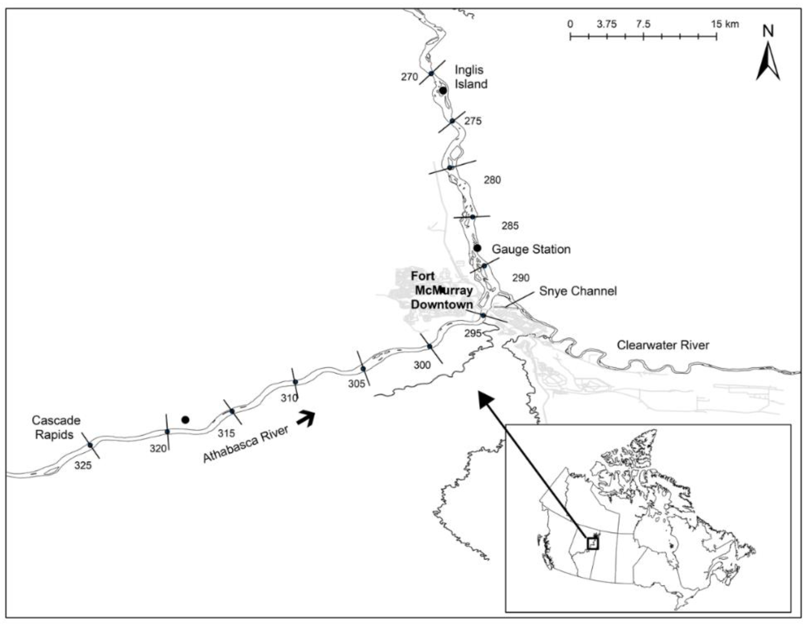
The river of interest is the Athabasca River in Alberta, Canada, which is approximately 1231 km long and flows from the Columbia Icefield at Jasper National Park in a northeasterly direction to Lake Athabasca at the Peace-Athabasca Delta. The model domain extends only along a lower stretch of the river, from Cascade Rapids to Inglis Island, a total of 51 km in length (Figure 1). The TFM is situated within the model domain at the confluence of the Athabasca and Clearwater rivers. The TFM is highly prone to ice-jam flooding due to the geomorphological setting of the river. Upstream of the TFM, the river is characterized by a steep slope, many rapids and high banks, while there is a relatively milder river slope with many islands and sandbars and low-lying riverbanks downstream of the TFM [37]. The Clearwater River has a major influence on the severity of ice-jam flooding as it can be an additional source of ice and water during spring break-up. Furthermore, the backwater from an ice jam on the Athabasca River downstream of the TFM can flow upstream into the Clearwater River to overflow banks and flood the downtown area of the TFM. Historically, several extreme ice-jam events occurred in 1875, 1977, 1978, 1979 and 2020. The most recent extreme ice-jam event, in 2020, was approximately 24 km long and flooded a substantial area of the downtown area of the TFM. More than 15,000 residences were evacuated and one human life was lost. Approximately 1200 properties were damaged [38] and the total damages from this flood event were estimated to be half a billion dollars.

A Water Survey of Canada hydrometric gauge station is located several kilometres downstream of the TFM, which records water level and flow discharge at 10 min intervals. The recorded water level and flow discharge data from this gauge station was used to establish maximum flow distributions and calibrate the inflowing volume of ice during spring ice-cover breakup for the stochastic modelling inputs.

3. Stochastic Modelling Framework

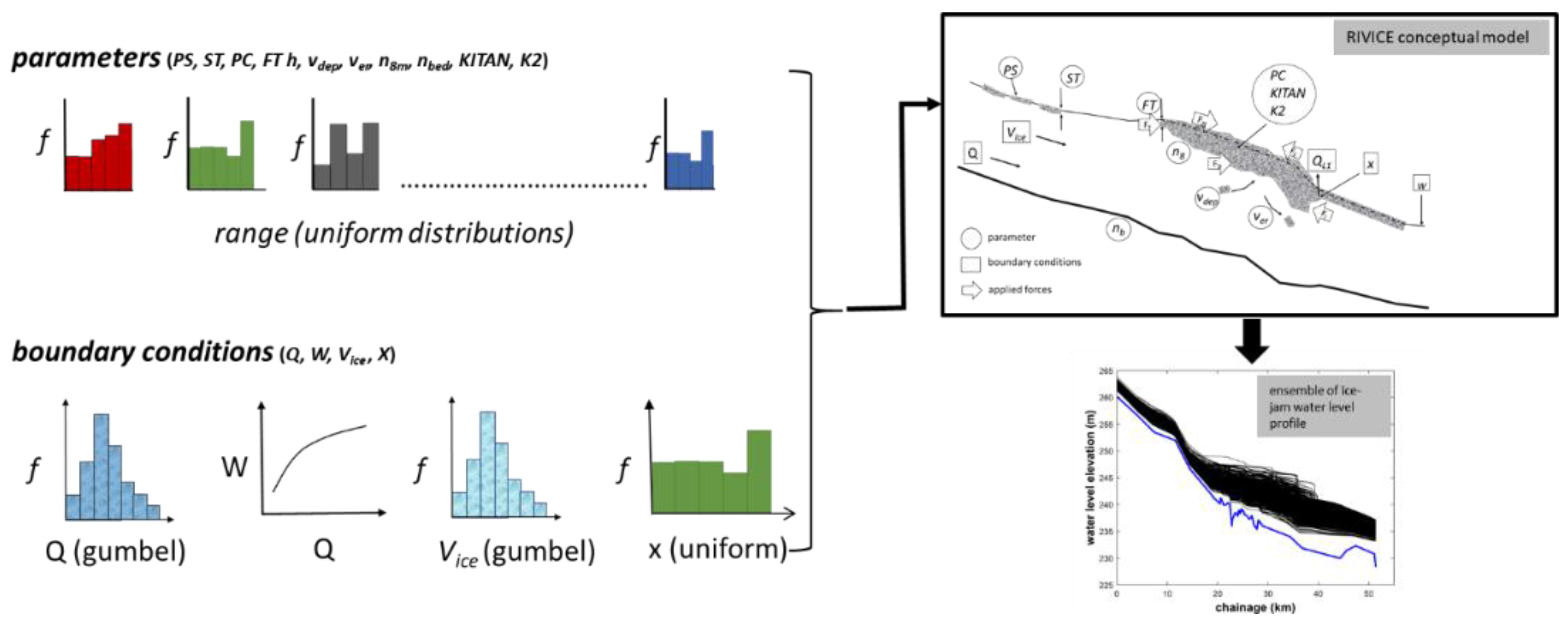
The ensemble of the base run simulation from a recent study by Das and Lindenschmidt [30] was used to determine the ice-jam flood risk for a hypothetical no-development zoning scenario along the Athabasca River at the TFM. In this study a hydraulic model, RIVICE, was placed in a stochastic modelling framework using a Monte-Carlo Analysis (MOCA). RIVICE is a fully dynamic one-dimensional river ice model, able to simulate river ice cover development, including frazil generation, border ice formation and breakup, including rate of ice-cover melting, ice-cover shoving and ice-jam formation. In this study, the ice cover initiation subroutine of the model was used to simulate ice jams based on a user-defined timing and lodgment location along the model domain. Surveyed cross-sections were primarily interpolated at 50 m spacing to set up the structure of the model. To simulate ice-jam scenarios, RIVICE requires the following inputs:

River discharge (Q), an upstream boundary condition input to the model, which can be incorporated as a daily/hourly hydrograph or an average value during simulations.

Inflowing volume of ice (V_ice), a user-defined boundary condition that allows a rate of incoming volume of ice to accumulate in an ice jam during each time step.

Toe of the ice-jam location (x), another user-defined boundary condition required to lodge an ice jam at a specific point along the model domain.

Porosity (PC) and thickness of ice-cover front (FT), ice-cover parameters defined by the user.

Porosity (PS) and thickness of slush pans (ST), rubble ice parameters also defined by the user.

Velocity threshold for the erosion of ice (v_er), introduced using either a critical velocity value or a tractive force criterion; the velocity threshold for the deposition of ice (v_dep) incorporates either a user-defined maximum velocity criterion, Meyer Perter Bed Load Analogy or deterministic Froude number. For example, if the deposition velocity is below a specified threshold, ice which is in transit is deposited under the stationary ice-cover; erosion of ice covers occurs when the specified flow velocity threshold is exceeded.

Riverbed roughness (n_bed), the hydraulic flow resistance parameterised by the Manning roughness coefficient; ice roughness (n_ice) is parameterised using one of three options—a method introduced by Beltaos [39], Nezhikhovskiy [40] or a user-defined constant.

Longitudinal to lateral force ratio (K1) and longitudinal to vertical force ratio (K2), user-defined to characterize the ice-jam cover strength.

A detailed description of how these parameters and boundary conditions are incorporated into the RIVICE programme is given in the software manual (http://giws.usask.ca/rivice/Manual/RIVICE_Manual_2013-01-11.pdf) and a recent publication [41]. Most of these inputs were calibrated using historical ice-jam events that occurred along the model domain. The detailed calibration and validation of RIVICE along the model domain is documented in a previous study by Lindenschmidt [41]. The calibrated RIVICE model is then placed into the MOCA framework to generate hundreds of ice-jam scenarios. MOCA was carried out using the Parameter Estimation Program (PEST) [42]. Since MOCA requires a different set of parameters and boundary conditions for each simulation, the values were extracted randomly from uniform or extreme value probability density functions. A uniform pdf was used for all the parameter values and the toe of the ice-jam location boundary condition, while the Gumbel distribution was used for the flow discharge and inflowing volume of ice (Figure 2). Available maximum flows during spring ice-cover breakup were selected to produce an extreme flow frequency distribution to extract random values for the MOCA simulations. The calibrated RIVICE model in the MOCA framework was initially run using an assumed value of inflowing ice distribution. The distribution was adjusted until the observed stage-frequency distribution matched the observed stage-frequency for ice jams at the Athabasca River gauge downstream of the TFM. After each MOCA simulation, the simulated stage-frequency distribution was compared with the observed stage-frequency distribution. If they did not coincide with one another, the corresponding ice distribution was adjusted and the MOCA was repeated. The process was repeated until agreement was attained between the two stage-frequency distributions. Once an ice distribution was calibrated, additional sets of MOCA runs were carried out to create an envelope of the ice distributions. Once all the model parameters and boundary conditions were randomly selected, a total of 379 ice-jam scenarios were simulated to estimate flood risk along the Athabasca River at Fort McMurray.

4. Flood Risk Estimation

Flood risk is defined as the probability of the adverse consequences of a flood event, which incorporates both flood hazard (flood intensity and probability of occurrence) and vulnerability (exposure and susceptibility). Flood intensity (flood depth and extent) was estimated by producing flood hazard maps from the simulated water level profiles and the probability of occurrence of each profile, calculated using the formula provided by Gerard and Karpuk [43]:

$$\mathrm{Exceedance} \mathrm{probability}, P\left(X\ge x\right)=\frac{m-\frac{3}{8}}{N+\frac{1}{4}}$$

(1)

where m is the rank of each ice-jam water level elevation, N is the total number of simulations and X is a value exceeding x [44].

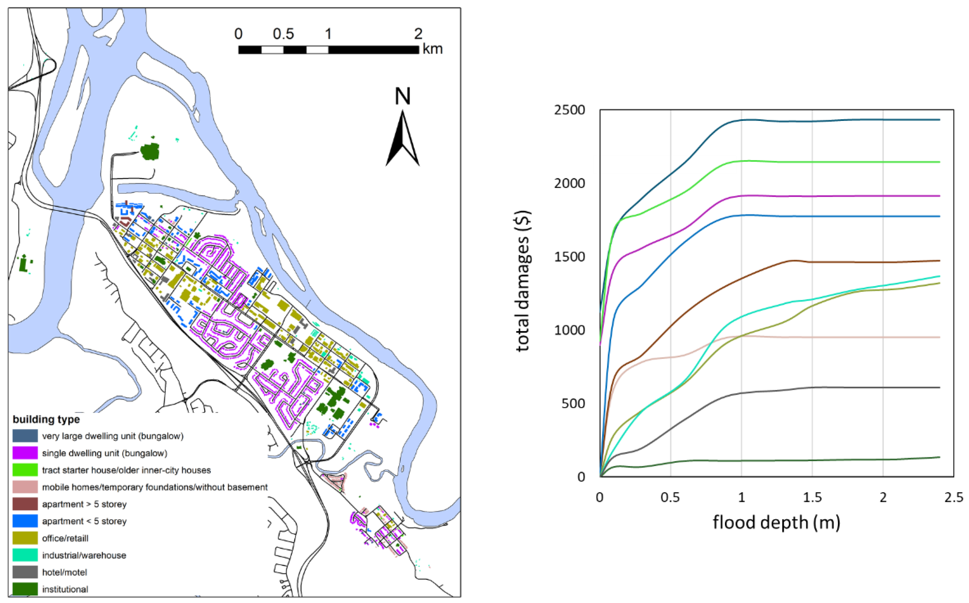
Exposure was calculated from land-use information (distribution of the buildings and their types), which was extracted from Google Earth using a geographic information system (GIS) tool (Figure 3). Susceptibility was determined using relationships between flood depths and structural and content damages, which were extracted from the information provided by a previous study [45] (Figure 3). Once all the information was derived, a flood risk map for each simulated water-level profile was developed and the total flood risk of each flood was then quantified. The EAD of the TFM was calculated using Equation (2). The EAD for the zoning regulation was then estimated by removing all the buildings in the zoning areas. The EAD for both the base run (no zoning) and mitigation (no development zoning) scenarios were compared to assess the effect of zoning ordinances on flood risk.

$$\mathrm{EAD} = {{\displaystyle \sum }}_{i=1}^{i=N}{P}_i \times D_i$$

(2)

where $P_i$ and $D_i$ are the exceedance probability and the total damages of each ice-jam flood event and N is the total number of simulations/events.

5. Global Sensitivity Analysis

A regional sensitivity analysis (RSA) was applied to understand the influence of model parameters and boundary conditions on the ice-jam flood risk [46]. In RSA, two distributions—behavioural and non-behavioural distributions for each parameter—are identified based on an objective function, which is often the model output. The behavioural and non-behavioural sets are selected based on a predefined threshold of the model output. Behavioural sets are those whose outputs closely represent the expected results or observed values (i.e., deviations are less than a threshold value), while non-behavioural parameters are designated to have deviations (model outputs are not closely aligned with the expected results or observed data) greater/less than the threshold value. Finally, the behavioural and non-behavioural cumulative distribution functions (CDF) are compared (a goodness-of-fit test) by superimposing them on a graph [47]. Greater dissimilarities between the behavioural and non-behavioural CDFs of a parameter indicate greater sensitivity of the parameter to the objective function.

The flood risk value of each simulated ice-jam profile for the TFM was used as an objective function in the global sensitivity analysis (GSA). Since the goal of the GSA in this study was to assess the influence of the model parameters and boundary conditions on the severity of ice-jam flood risk, 10% of the highest risk values were labelled as behavioural, while the rest were classified as non-behavioural. The cumulative distribution of the behavioural and non-behavioural values for the parameters and boundary conditions were then compared graphically and statistically. The graphical superimposed CDFs of each parameter provide a visual assessment of the level of sensitivity in the whole parameter range. The classical Kolmogorov-Smirnov (K-S) distance measurement [48] was used to rank the parameter and boundary condition sensitivities quantitatively.

6. Impact of Zoning on the Flood Risk at TFM

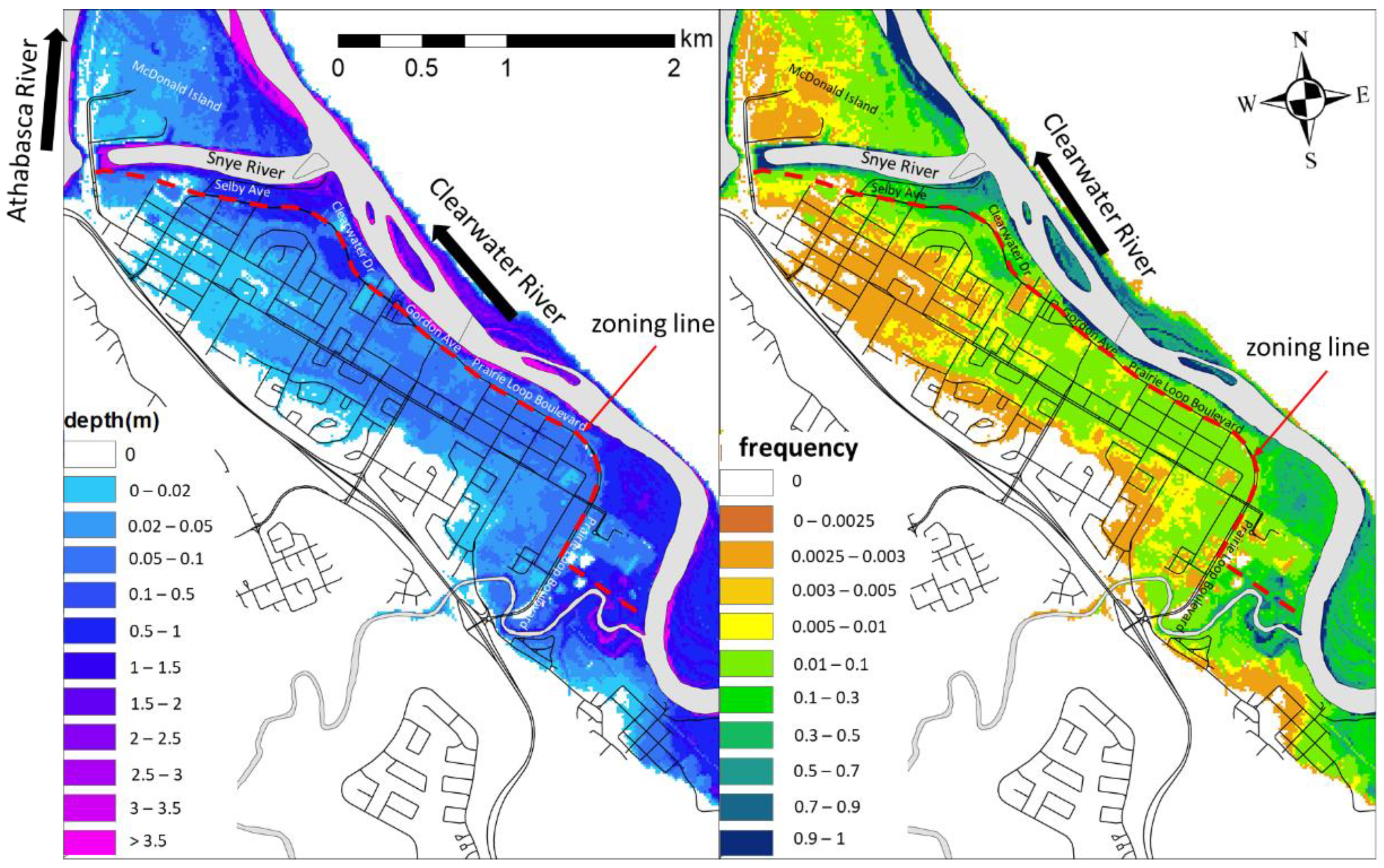
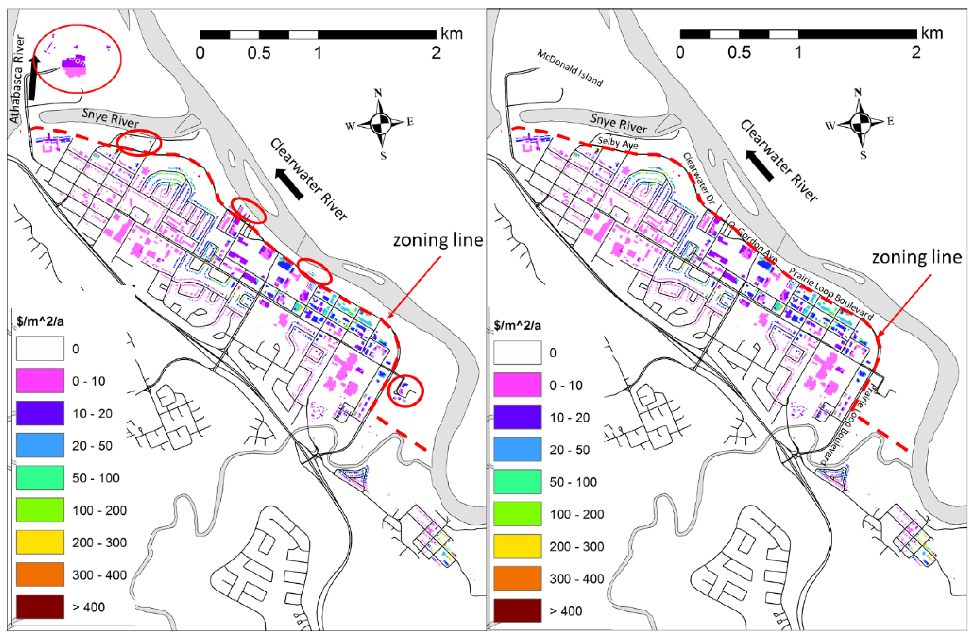
Figure 4 presents the flood intensity maps and zoning line for the TFM. Flood intensity maps demonstrate the average flood depth and extent, and the frequency of flooding along the TFM. The frequency of flooding indicates the probable vulnerable areas of the TFM, calculated as the total number of times the areas were flooded divided by the total number of the ice-jam simulations. These maps were extracted from a recent publication by Das and Lindenschmidt [30].

The zoning ordinance area was selected subjectively and extended from Selby Avenue along the Snye River to Clearwater Drive, Gordon Avenue and Prairie Loop Boulevard adjacent to the Clearwater River. Along the river side of the zoning line, the TFM is highly vulnerable to all high-frequency floods. In particular, there are some residential and recreational buildings that are highly vulnerable to ice-jam floods. Impacts of these buildings on ice-jam flood risk can be evaluated by calculating the total expected annual damages (EAD) from the no-development zoning runs and then applying the zoning ordinance.

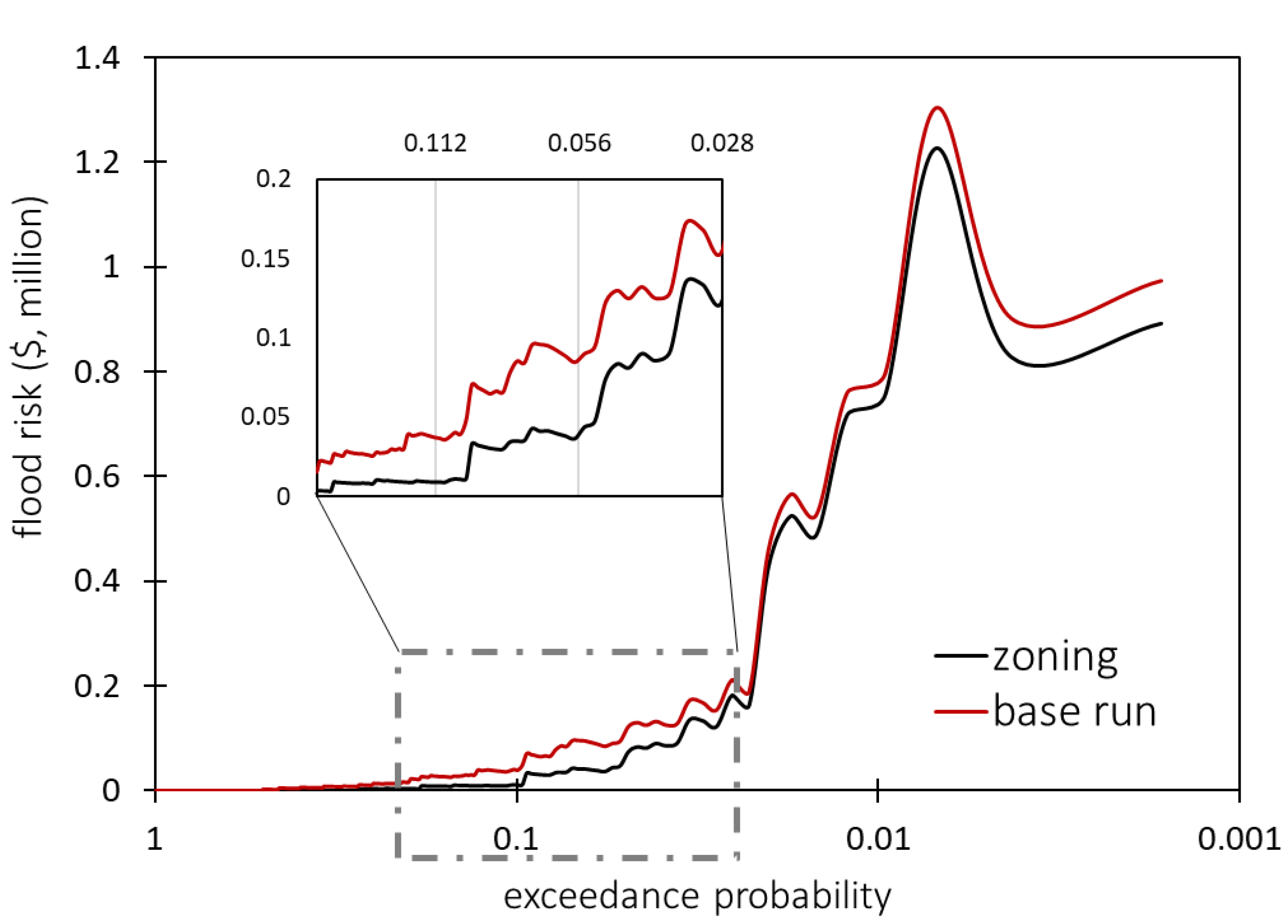
Flood risk of the base run (no zoning) scenario was established with the presence of all the buildings under a certain flood depth, while the no-development zoning scenario was developed by removing all the buildings that exist in the zoned area. A detailed analysis of the exceedance probability and flood risk of each simulated flood for the base run and no development zoning scenarios is presented in Figure 5. The result shows that zoning could substantially reduce the total flood risk for high-frequency flood events, an almost 50% reduction in flood risk for the events with exceedance probability from 0.028 (1:35 year) to 0.2 (1:5 year). This is due to the fact that fewer extreme flood events, which are highly probable in the zoned area, cause excessive damages to the existing buildings. Moreover, more extreme flooding can still inundate the area beyond the zoned area and result in high damages to buildings in the TFM. However, zoning is still effective to reduce a certain level of flood risk for more extreme ice-jam flood events.

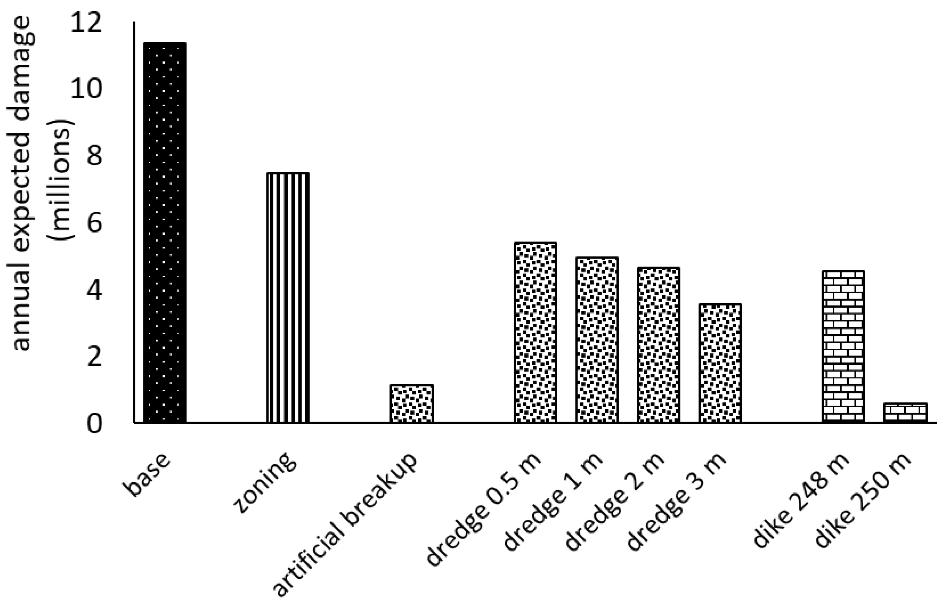
The annual risk maps and EADs for both the no-zoning run and zoning scenarios are presented in Figure 6. The maps show the annual flood risk of each building in the TFM. Moreover, the bar graph of the total EADs illustrates that although other mitigation scenarios are still relatively efficient at reducing EAD, zoning ordinances could also reduce a substantial amount of EAD. The EAD for the no-zoning scenario is about $11.4 million, which is reduced to $7.5 million (34%) after applying the zoning regulation (see Figure 7).

7. Sensitivity of Model Parameters and Boundary Conditions

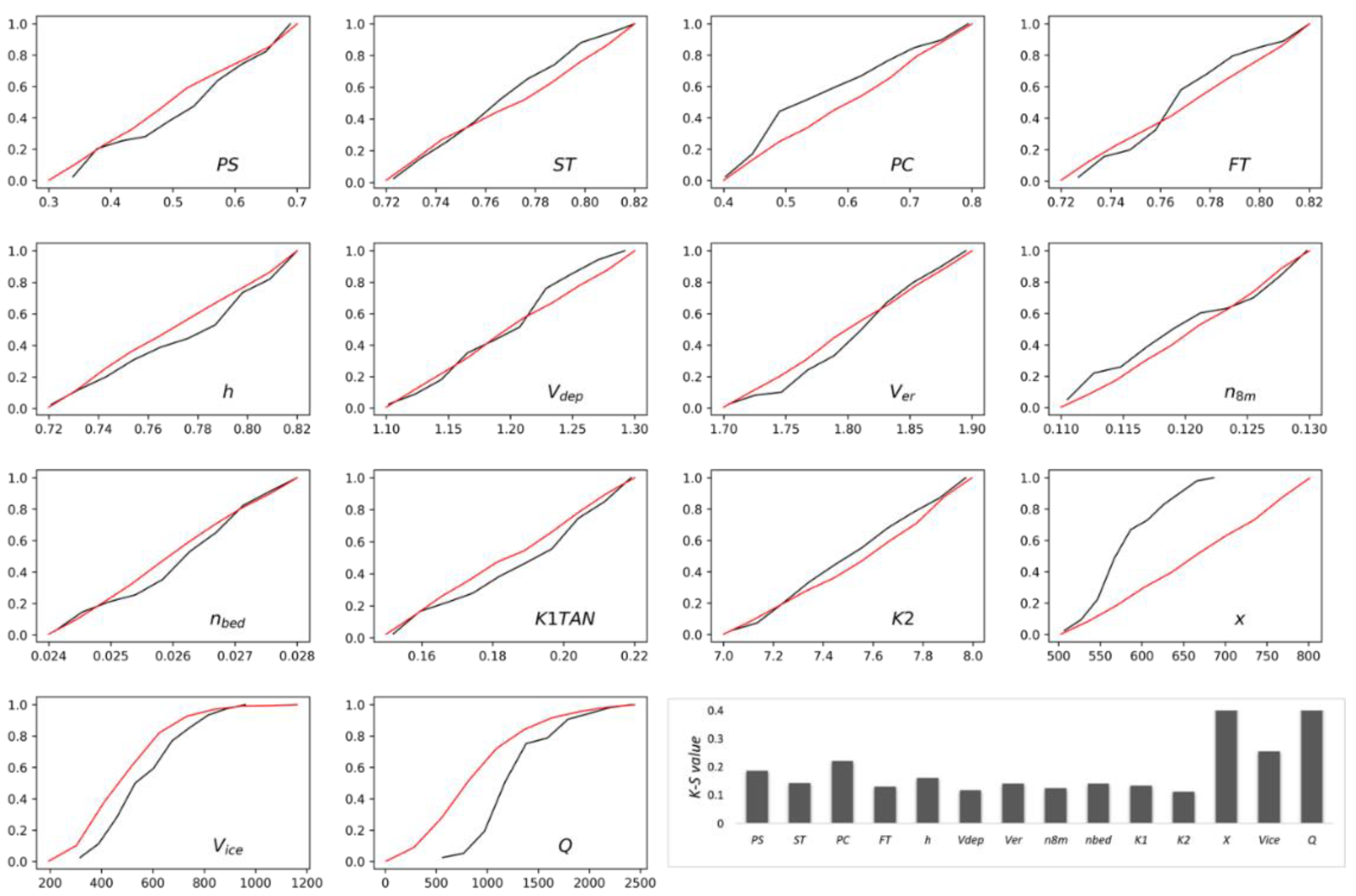
Since the ensemble of flood hazard maps provides an ensemble of flood risk values, these values were used in the GSA to assess the impacts of model parameters and boundary conditions on flood risk. Figure 8 illustrates the flood risk sensitivity to model parameters and boundary conditions. The parameters and boundary condition sets were selected based on the flood risk—the parameter and boundary condition sets that produced the highest 10% of the flood risk were selected as behavioural and the rest of the sets were selected as non-behavioural distributions. The results show that flood risk is not very sensitive to model parameters, while it is highly sensitive to all the boundary conditions. The ranking bar graph shows that flood risk has low to moderately sensitivity to model parameters and high sensitivity to boundary conditions. The highly influential boundary conditions, such as upstream discharge, the volume of incoming ice floes and the toe of ice jam locations, are very important for ice-jam flood risk estimations. Therefore, all these boundary conditions have a great influence on the hydraulic and physical processes of ice-jam formation, subsequent flooding and severity of flood risk. For example, a different location of the toe of the ice jam changes the physical characteristics of an ice jam due to geomorphological variations along the river channel. Moreover, varying discharges and volumes of inflowing ice can also change the hydraulic and physical characteristics of the jam. Thus, they can change the effects of ice-jam-induced backwater staging and the degree of severity of ice-jam flooding.

8. Conclusions

A stochastic modelling approach was applied to evaluate a hypothetical zoning regulation measure to reduce ice-jam flood risk along the Athabasca River at the TFM. The studied zoning areas have a significant potential to reduce the overall flood risk for most of the high-frequency flood events. Although these high-frequency flood events are less extreme, they can still result in a substantial level of flood risk as there are many buildings and recreational facilities in the zoning area that are highly vulnerable to ice-jam flood hazards. A similar approach was applied to assess several other mitigation measures, such as sediment dredging, artificial breakup and dike construction around the TFM to reduce ice-jam flood risk at the TFM [30]. The study concluded that a 250 m a.s.l. crest-elevation dike has the highest potential to reduce EAD at the TFM. However, a dike height that has been proposed along the zoning area may not be able to reduce the flood risk if there is still development planned in the zoning areas. Therefore, combined measures, such as zoning and a dike, could be implemented to reduce the maximum flood risk at the TFM.

A global sensitivity analysis (GSA) provided comprehensive diagnostic insight into the hydraulic model parameters and boundary conditions. This study identified that ice-jam flood risk is highly sensitive to the model boundary conditions (stream discharge, the volume of ice and toe of ice jam location). The results could help in resource allocation for data collection and further ice-jam flood modelling studies, such as determining which ranges of parameter and boundary conditions may have higher impacts on ice-jam flood risk within the model domain.

There are some uncertainties and limitations associated with the modelling framework and input data. Some anthropogenic changes, such as land-use data and depth-damage relationships, could also affect the overall flood risk results. For example, the land-use data for downtown Fort McMurray was extracted from a Google Earth image acquired in 2016 and there could have been additional development or changes in the landscape since that time. In addition, some of the developments may not have existed in 1977, which has implications for the flood risk calibration. Moreover, the depth-damage curves used in the analyses were derived using market values from 2014. However, none of the above factors would likely alter the overall result that zoning could substantially reduce the overall flood risk.

References

- Beltaos, S.; River, I.J. River Ice Jams; Water Resources Publication: Littleton, CO, USA, 1995. [Google Scholar]
- Beltaos, S.; Burrell, B.C. Extreme Ice Jam Floods along the Saint John River; IAHS Publication: Wallingford, UK, 2002. [Google Scholar]
- Munck, S.D.; Gauthier, Y.; Bernier, M.; Chokmani, K.; Légaré, S. River predisposition to ice jams: A simplified geospatial model. Nat. Hazards Earth Syst. Sci. 2017, 17, 1033–1045. [Google Scholar] [CrossRef] [Green Version]
- Healy, D.; Hicks, F.E. Experimental study of ice jam formation dynamics. J. Cold Reg. Eng. 2006, 20, 117–139. [Google Scholar] [CrossRef]
- Scrimgeour, G.J.; Prowse, T.D.; Culp, J.M.; Chambers, P.A. Ecological effects of river ice break-up: A review and perspective. Freshw. Biol. 1994, 32, 261–275. [Google Scholar] [CrossRef]
- Beltaos, S. Onset of river ice breakup. Cold Reg. Sci. Technol. 1997, 25, 183–196. [Google Scholar] [CrossRef]
- Rokaya, P.; Budhathoki, S.; Lindenschmidt, K.E. Trends in the timing and magnitude of ice-jam floods in Canada. Sci. Rep. 2018, 8, 1–9. [Google Scholar] [CrossRef] [PubMed] [Green Version]
- Madaeni, F.; Lhissou, R.; Chokmani, K.; Raymond, S.; Gauthier, Y. Ice jam formation, breakup and prediction methods based on hydroclimatic data using artificial intelligence: A review. Cold Reg. Sci. Technol. 2020, 174, 103032. [Google Scholar] [CrossRef]
- Burrell, B.; Huokuna, M.; Beltaos, S.; Kovachis, N.; Turcotte, B.; Jasek, M. Flood Hazard and Risk Delineation of Ice-Related Floods: Present Status and Outlook. In Proceedings of the 18th CGUHS CRIPE Workshop on the Hydraulics of Ice Covered Rivers, Quebec City, QC, Canada, 18–20 August 2015. [Google Scholar]
- Carson, R.; Beltaos, S.; Groeneveld, J.; Healy, D.; She, Y.; Malenchak, J.; Shen, H.T. Comparative testing of numerical models of river ice jams. Can. J. Civ. Eng. 2011, 38, 669–678. [Google Scholar] [CrossRef]
- US-Army. HEC-2 Water Surface Profiles, Hydrologic Engineering Center. US Army Corps of Engineers, Davis, California. This is the First Version of the Program HEC-2 for Calculating the Hydraulics of Open-Channel Flow; Water Resources Support Center, Hydrologic Engineering Center: Davis, CA, USA, 1990. [Google Scholar]
- Beltaos, S. User’s Manual for the RIVJAM Model; National Water Research Institute Contribution 96-37; National Water Research Institute: Burlington, ON, Canada, 1996. [Google Scholar]
- Healy, D. Hicks, F. Comparison of ICEJAM and RIVJAM ice jam profile models. J. Cold Reg. Eng. 1999, 13, 180–198. [Google Scholar] [CrossRef] [Green Version]
- Shen, H.T.; Wang, D.S.; Lal, A.W. Numerical simulation of river ice processes. J. Cold Reg. Eng. 1995, 9, 107–118. [Google Scholar] [CrossRef]
- EC. RIVICE Model—User’s Manual. 2013. Available online: http://giws.usask.ca/rivice/Manual/RIVICE_Manual_2013-01-11.pdf (accessed on 1 June 2021).
- Liu, L.; Li, H.; Shen, H.T. A two-dimensional comprehensive river ice model. In Proceedings of the 18th IAHR Symposium on River Ice, Sapporo, Japan, 28 August–1 September 2006; Volume 28. [Google Scholar]
- Beltaos, S. Assessing ice-jam flood risk: Methodology and limitations. In Proceedings of the 20th IAHR Inernational Symposium on Ice, Lathi, Finland, 14–18 June 2010; pp. 14–17. [Google Scholar]
- Lindenschmidt, K.-E.; Das, A.; Rokaya, P.; Chu, T. Ice-jam flood risk assessment and mapping. Hydrol. Process. 2016, 30, 3754–3769. [Google Scholar] [CrossRef]
- Alaghmand, S.; Bin Abdullah, R.; Abustan, I.; Eslamian, S. Comparison between capabilities of HEC-RAS and MIKE11 hydraulic models in river flood risk modelling (a case study of Sungai Kayu Ara River basin, Malaysia). Int. J. Hydrol. Sci. Technol. 2012, 2, 270–291. [Google Scholar] [CrossRef]
- Beltaos, S. Comparing the impacts of regulation and climate on ice-jam flooding of the Peace-Athabasca Delta. Cold Reg. Sci. Technol. 2014, 108, 49–58. [Google Scholar] [CrossRef]
- Wolfe, B.B.; Hall, R.I.; Wiklund, J.A.; Kay, M.L. Past variation in Lower Peace River ice-jam flood frequency. Environ. Rev. 2020, 28, 209–217. [Google Scholar] [CrossRef] [Green Version]
- Goldberg, M.D.; Li, S.; Lindsey, D.T.; Sjoberg, W.; Zhou, L.; Sun, D. Mapping, Monitoring, and Prediction of Floods Due to Ice Jam and Snowmelt with Operational Weather Satellites. Remote. Sens. 2020, 12, 1865. [Google Scholar] [CrossRef]
- Lindenschmidt, K.-E.; Rokaya, P.; Das, A.; Li, Z.; Richard, D. A novel stochastic modelling approach for operational real-time ice-jam flood forecasting. J. Hydrol. 2019, 575, 381–394. [Google Scholar] [CrossRef]
- Andrishak, R.; Hicks, F. Simulating the effects of climate change on the ice regime of the Peace River. Can. J. Civ. Eng. 2008, 35, 461–472. [Google Scholar] [CrossRef]
- Turcotte, B.; Morse, B.; Pelchat, G. Impact of Climate Change on the Frequency of Dynamic Breakup Events and on the Risk of Ice-Jam Floods in Quebec, Canada. Water 2020, 12, 2891. [Google Scholar] [CrossRef]
- Das, A.; Rokaya, P.; Lindenschmidt, K.E. Ice-jam flood risk assessment and hazard mapping under future climate. J. Water Resour. Plan. Manag. 2020, 146, 04020029. [Google Scholar] [CrossRef]
- Vogel, R.M.; Stedinger, J.R. Flood-Plain delineation in ice jam prone regions. J. Water Resour. Plan. Manag. 1984, 110, 206–219. [Google Scholar] [CrossRef]
- Beltaos, S. Progress in the study and management of river ice jams. Cold Reg. Sci. Technol. 2008, 51, 2–19. [Google Scholar] [CrossRef]
- Kovachis, N.; Burrell, B.C.; Huokuna, M.; Beltaos, S.; Turcotte, B.; Jasek, M. Ice-jam flood delineation: Challenges and research needs. Can. Water Resour. J. Rev. Can. Ressour. Hydr. 2017, 42, 258–268. [Google Scholar] [CrossRef]
- Das, A.; Lindenschmidt, K.E. Evaluation of the implications of ice-jam flood mitigation measures. J. Flood Risk Manag. 2021, 14, e12697. [Google Scholar] [CrossRef]
- Doberstein, B.; Fitzgibbons, J.; Mitchell, C. Protect, accommodate, retreat or avoid (PARA): Canadian community options for flood disaster risk reduction and flood resilience. Nat. Hazards 2019, 98, 31–50. [Google Scholar] [CrossRef]
- Wagener, T.; Pianosi, F. What has Global Sensitivity Analysis ever done for us? A systematic review to support scientific advancement and to inform policy-making in earth system modelling. Earth-Sci. Rev. 2019, 194, 1–18. [Google Scholar] [CrossRef]
- Zhou, X.; Lin, H. Global Sensitivity Analysis. In Encyclopedia of GIS; Shekhar, S., Xiong, H., Zhou, X., Eds.; Springer International Publishing: Cham, Switzerland, 2017. [Google Scholar]
- Pianosi, F.; Wagener, T. A simple and efficient method for global sensitivity analysis based on cumulative distribution functions. Environ. Model. Softw. 2015, 67, 1–11. [Google Scholar] [CrossRef] [Green Version]
- Das, A.; Lindenschmidt, K.E. Evaluation of the sensitivity of hydraulic model parameters, boundary conditions and digital elevation models on ice-jam flood delineation. Cold Reg. Sci. Technol. 2021, 183, 103218. [Google Scholar] [CrossRef]
- Sheikholeslami, R.; Yassin, F.; Lindenschmidt, K.E.; Razavi, S. Improved understanding of river ice processes using global sensitivity analysis approaches. J. Hydrol. Eng. 2017, 22, 04017048. [Google Scholar] [CrossRef]
- She, Y.; Andrishak, R.; Hicks, F.; Morse, B.; Stander, E.; Krath, C.; Mahabir, C. Athabasca River ice jam formation and release events in 2006 and 2007. Cold Reg. Sci. Technol. 2009, 55, 249–261. [Google Scholar] [CrossRef]
- Antoneshyn, A. Fort McMurray flood damages top $500M. 2020. Available online: https://edmonton.ctvnews.ca/fort-mcmurray-flood-damages-top-500m-1.5051023 (accessed on 9 August 2021).
- Beltaos, S.; Burrell, B.C. Ice-jam model testing: Matapedia River case studies, 1994 and 1995. Cold Reg. Sci. Technol. 2010, 60, 29–39. [Google Scholar] [CrossRef]
- Nezhikhovskiy, R.A. Coefficients of roughness of bottom surface on slush-ice cover. In Soviet Hydrology; American Geophysical Union: Washington, DC, USA, 1964; pp. 127–150. [Google Scholar]
- Lindenschmidt, K.E. RIVICE—A non-proprietary, open-source, one-dimensional river-ice model. Water 2017, 9, 314. [Google Scholar] [CrossRef]
- Doherty, J. Calibration and Uncertainty Analysis for Complex Environmental Models. In Watermark Numerical Computing; Watermark Numerical Computing is the Publisher: Brisbane, Australia, 2015; ISBN 978-0-9943786-0-6. [Google Scholar]
- Gerard, R.; Karpuk, E.W. Probability analysis of historical flood data. J. Hydraul. Div. 1979, 105, 1153–1165. [Google Scholar] [CrossRef]
- White, K.; Beltaos, S. Chapter 9: Development of ice-affected stage frequency curves. Highlands Ranch. In River Ice Break-Up; Water Resources Publications: Littleton, CO, USA, 2008. [Google Scholar]
- IBI and Golder Associates Ltd. Report Feasibility Study—Athabasca River Basins. Prepared for Government of Alberta—Flood Recovery Task Force. 2014. Available online: https://open.alberta.ca/publications/35751 (accessed on 11 August 2021).
- Hall, J.; Boyce, S.; Wang, Y.; Dawson, R.; Tarantola, S.; Saltelli, A. Sensitivity analysis for hydraulic models. J. Hydraul. Eng. 2009, 135, 959–969. [Google Scholar] [CrossRef]
- Thompson, S.A. Hydrology for Water Management; CRC Press: Boca Raton, FL, USA, 2017. [Google Scholar]
- Stephens, M.A. Introduction to Kolmogorov (1933) on the empirical determination of a distribution. In Breakthroughs in Statistics. Springer Series in Statistics (Perspectives in Statistics); Kotz, G., Johnson, N.L., Eds.; Springer: New York, NY, USA, 1992. [Google Scholar]
- Das, A. Stochastic Modelling Approach to Improve Ice-Jam Flood Risk Management. Ph.D. Thesis, University of Saskatchewan, Saskatoon, SK, Canada, 2021. [Google Scholar]
Figure 1.
Study site of the Lower Athabasca River. The km values are marked along the model domain from Cascade Rapids to Inglis Island.
Figure 2.
Stochastic modelling framework to simulate ice-jam scenarios.
Figure 3.
Distribution of different types of buildings (left panel) and depth-damage relationships for structure and content of various types of buildings (right panel) at the TFM.
Figure 4.
Flood hazard maps indicating the zoning line along the Athabasca River at the TFM (The flood hazard maps were adopted from Das and Lindenschmidt, 2021 (used with permission) and modified here to assess zoning regulation).
Figure 5.
The flood risk contribution and exceedance probability of each flood from no-development zoning and base run scenarios.
Figure 6.
Annual flood risk maps and total EADs for the zoned (right panel) and no-zoning scenarios (left panel), the red circles indicates the properties under a specific flood risk in the zoning area. (The risk map was adopted from Das and Lindenschmidt, 2021b (used with permission) and modified here to assess zoning regulation).
Figure 7.
The expected annual damages for different mitigation scenarios (the figure is adopted from [30,49] (used with permission) and modified here by adding the annual expected damage for the zoning regulation).
Figure 8.
Cumulative distribution plots of behavioural (black) and non-behavioural (red) and K-S values for the model parameters and boundary conditions.
Publisher’s Note: MDPI stays neutral with regard to jurisdictional claims in published maps and institutional affiliations. |
© 2021 by the authors. Licensee MDPI, Basel, Switzerland. This article is an open access article distributed under the terms and conditions of the Creative Commons Attribution (CC BY) license (https://creativecommons.org/licenses/by/4.0/).
Share and Cite
MDPI and ACS Style
Das, A.; Lindenschmidt, K.-E. Exploring the Potential of Zoning Regulation for Reducing Ice-Jam Flood Risk Using a Stochastic Modelling Framework. Water 2021, 13, 2202. https://doi.org/10.3390/w13162202
AMA Style
Das A, Lindenschmidt K-E. Exploring the Potential of Zoning Regulation for Reducing Ice-Jam Flood Risk Using a Stochastic Modelling Framework. Water. 2021; 13(16):2202. https://doi.org/10.3390/w13162202
Chicago/Turabian StyleDas, Apurba, and Karl-Erich Lindenschmidt. 2021. "Exploring the Potential of Zoning Regulation for Reducing Ice-Jam Flood Risk Using a Stochastic Modelling Framework" Water 13, no. 16: 2202. https://doi.org/10.3390/w13162202
Note that from the first issue of 2016, this journal uses article numbers instead of page numbers. See further details here.