
Spatial Variations in Water-Holding Capacity as Evidence of the Need for Precision Irrigation
by
 ,
,
Mohd Shahkhirat Norizan
1,*, 
Aimrun Wayayok
2,3,*,
Ahmad Fikri Abdullah
2,3,
Muhammad Razif Mahadi
2,3 and
Yahya Abd Karim
4 1
Agronomy Department, FGV R&D Sdn Bhd, PPP Tun Razak, Bandar Pusat Jengka 26400, Pahang, Malaysia
2
Department of Biological and Agricultural Engineering, Faculty of Engineering, Universiti Putra Malaysia, Serdang 43400, Selangor, Malaysia
3
SMART Farming Technology Research Center, Faculty of Engineering, Universiti Putra Malaysia, Serdang 43400, Selangor, Malaysia
4
FGV R&D Sdn Bhd, Level 9 WEST, Wisma FGV, Jalan Raja Laut, Kuala Lumpur 50350, Malaysia
*
Authors to whom correspondence should be addressed.
Water 2021, 13(16), 2208; https://doi.org/10.3390/w13162208
Submission received: 29 June 2021
/
Revised: 10 August 2021
/
Accepted: 11 August 2021
/
Published: 13 August 2021
(This article belongs to the Special Issue Research on Soil Water Balance)
Abstract
:Malaysia receives a lot of water from its two main monsoon periods. Generally, there is a lot of precipitation throughout the year, with drought periods lasting less than three months. To date, irrigation has been treated homogenously, even though soil properties can vary spatially over a field, requiring site-specific applications. The aim of this study was to establish an irrigation management zone (IMZ) covering 23.4 ha, which was previously determined under the same soil series. Soil sampling was done according to a grid system over an area of 100 m × 100 m. Three soil depth ranges were examined for every sampling point, namely 0–30, 30–60, and 60–90 cm from the soil surface. Samples were taken to a laboratory for physical analysis and determination of the available water-holding capacity (AWHC). Delineation of AWHC values was achieved using GIS software and the Kriging method. Estimated irrigation depth (EID) data for the plantation were collected for the years 2016 and 2017. Afterward, EID and total net irrigation (TNI) data were simulated in the FAO Cropwat model and compared. The results showed that clay, sand, and organic matter (OM) distributions varied with soil depth; however, no strong correlation was found between these variable with AWHC. The IMZ was classified into three areas named zones A, B, and C, ranging from 79 to 167 mm. The crop water requirement (CWR) was 667 mm in 2016 but only 260 mm in 2017. Based on the AWHC values, the EID for 2016 was found to be below the TNI requirement range of about 106 to 110 mm. In contrast, the EID range was approximately 34 to 62 mm and above TNI requirements for 2017. This study indicates that water inputs for irrigation can be optimized with knowledge of the water-holding capacity of a specific soil. Subsequently, this can be related to crop yield and the impact on sustainable agriculture.
1. Introduction
Water is the most important resource on earth; however, over 96.5% of the water on earth is saline, while the remainder is freshwater. A total of 68.6% of freshwater is locked up in the form of ice and glaciers, while another 30.1% is stored as ground water [1]. The human population keeps is continually increasing, reaching 7.9 billion people in 2020 [2] and being predicted to increase by 22 to 34% by 2050 [3]; therefore, water security, i.e., having access to an adequate quantity and acceptable quality of water, is already at risk and will become worse over the next few decades [4]. Water resources are undoubtedly declining at an alarming rate all around the world [5]. Valipour et al. [6] showed that the global mean surface temperature increased by 0.66 °C for the periods of 1961–1990 to 2000–2019. This parameter is the most important indicator of global warming and climate change. Climate change substantially impacts developing countries and can be felt through impacts on water supply, food security, and agricultural incomes [7]; therefore, irrigation planning and water management policies need to be reviewed systematically.
Malaysia is experiencing exceptional stress on its water supply; however, 68% of water used in agriculture is still being managed inefficiently [8]. Based on projections, almost 46% of the water demand in Peninsula Malaysia or 8.39 billion m3 will be solely used for irrigation in 2050 [9]. To prepare for such an eventuality, it is expected that the focus will shift to improving water usage management rather than water supply management [10].
Agricultural production must also keep pace with the upward trend in human population growth. In Malaysia, oil palm serves as an important commodity crop, accounting for 37.7% of the gross output for the agriculture sector [11]. Worldwide consumption of palm oil has steadily increased, reaching about 75.45 Million MT for the 2020–2021 period [12]. Oil palm is considered as a robust plant that is able to grow under multiple abiotic stresses; however, in order to get the potential yield, every single factor that translates into yield is essential. Soil with low water-holding capacity is one of the major problems facing the industry, as this will result in low nutrient uptake, especially during the dry season. In addition, low water availability reduces the sex ratio and yield tonnage. To increase water availability, irrigation is used, although this requires a high initial cost per unit area.
The result from a series of irrigation trials at Serting (Central Peninsula of Malaysia) showed that irrigation in seasonal dry periods may increase yields by up to 56% compared with no irrigation [13]; however, another study in a moderately wet area showed that irrigation only resulted in a small improvement of 9% compared to a non-irrigated plot [14]. This shows that with correct area selection, irrigation may give a good response. Irrigation generally requires high initial costs, as it is necessary to set up water pumps, reservoirs, and piping networks, as well as requiring special workers and periodic maintenance of parts. For oil palm, it has been reported that the total costs amount to USD 1680 per ha for furrow systems [13]; in fact, these costs increase every year. Without thorough selection criteria, an irrigation project may end up being unprofitable or requiring a longer time to achieve a high return of investment (ROI) rate.
In general, the amount of rainfall and the soil characteristics are often used as basic criteria for determination of irrigation events. If a farmers applies a large amount of water in a field, this may be more than enough or the field may be undersupplied. The question regarding water efficiency for using irrigation still needs to be answered, as water management schemes could become important in the future [15]. The palm oil industry in Malaysia is subject to rules and regulations set by the Roundtable on Sustainable Palm Oil (RSPO). Under Principle 7 (Protect, Conserve, and Enhance Ecosystems and the Environment), water as one of the key resources needs to be used efficiently [16]. Recently, studies related to water footprints were carried out [17,18], helping improve the understanding of water usage.
After considering the aforementioned factors, it stands to reason that water must be used wisely. One strategy to increase water use efficiency is to adopt precision irrigation (PI) in the field. The traditional practice of using rainfall for irrigation absolutely needs to be improved. PI concepts are quite new in the oil palm industry and no detailed studies have described their effectiveness or profitability or have proven how these concepts can be useful in oil palm plantations. Such approaches must be combined with soil, rainfall, and meteorological data, as well as current oil palm conditions. As such, this study was carried out to determine the spatial variability within an irrigation area and to evaluate existing irrigation projects based on climate and water-holding capacity. The hypothesis was that a higher soil water-holding capacity will lead to soil moisture retention over a longer time and less irrigation water being required. By doing this, water usage and irrigation requirements can be achieved. This study gives an idea of the necessity of using precision irrigation strategies for particular areas. Finally, estate management teams can adopt related technology such as soil moisture sensors to achieve better irrigation management.
2. Materials and Methods
2.1. Study Area
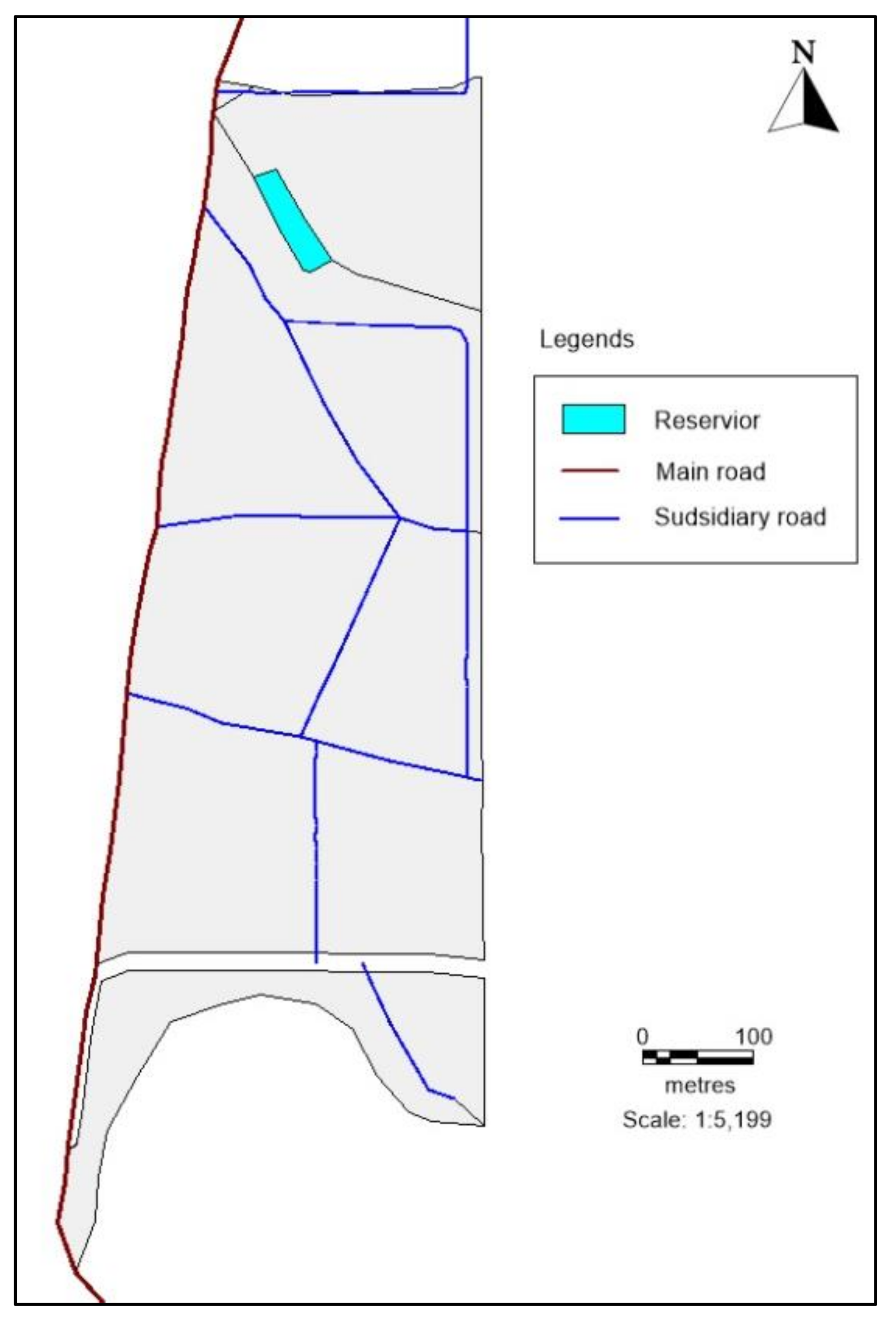
A semi-commercial irrigation system was implemented at FGV Agri Services Sdn Bhd (FGVAS) Serting Hilir Estate, located at the center of Peninsula Malaysia (2°56’51” N, 102°29’20” E) (Figure 1). Oil palm was obtained from commercial clonal material and planted with a density of 148 palms ha−1. The soil was classified as Typic Kandiudult, with fine loamy, kaolinitic, and isohyperthermic or Haplic Acrisol characteristics, using the Food and Agriculture Organization (FAO) legend [19]. The soil developed over recent riverine alluvium and was considered as having low fertility.
2.2. Estate Irrigation Practices
Water has been delivered to the palms using a microsprayer irrigation system since 2015, although only fully commenced from 2016. One emitter was installed for every palm on a lateral polyethylene (PE) pipe. The average output of each emitter is 60 Lh−1. The total irrigation area covers 23.4 ha, which was eventually divided into three working areas. Irrigation events are decided based on the amount of rainfall from the previous day (an irrigation event requires rainfall below 5.0 mm on the previous day). The system operates manually, although the engine automatically stops at the end of each shift. The operation time for each shift was approximately two and a half hours.
Based on the operation hours, the estimated volume of water (EVW) in liters was calculated for a particular year (Equation (1)) and later converted into the estimated irrigation depth (EID) in mm, as calculated using Equation (2). The EVW is quite straightforward, involving the monthly operation time in hours (T), area of irrigation (A) in ha, number of emitters (N) per ha, and nominal emitter flow rate (F) in Lh−1; however, the EID involves the area occupied oil palms based on the canopy radius (r) in m [20] and the density of palms per ha (D). In 2016, the palms were three years old and the value of r was set at 3.43 m, while in 2017 the value of r was 4.58 m [21].
EVW = (T × A × N × F)
2.3. Meteorological Data Collection
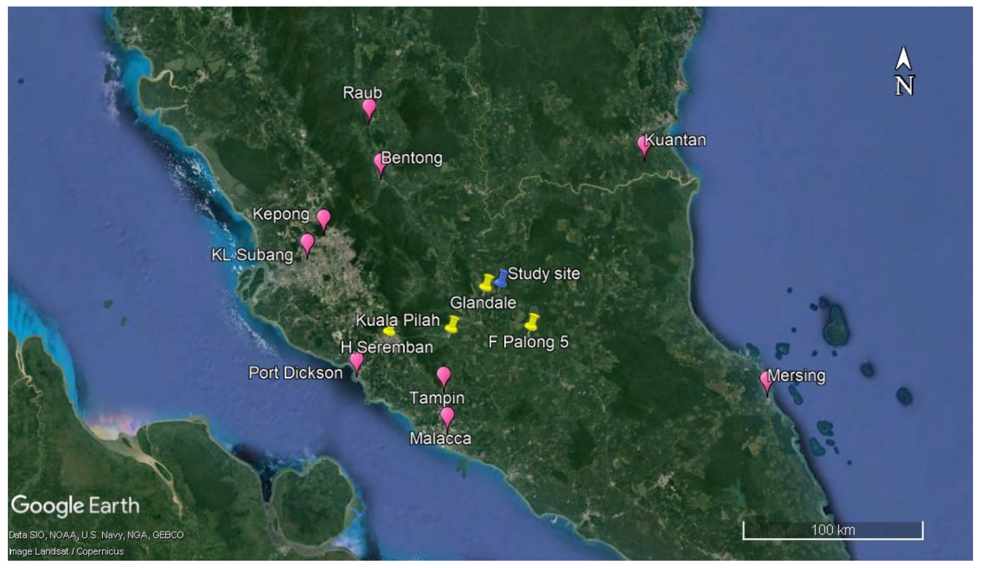
The FAO Cropwat model was used to estimate the reference evapotranspiration (ETo) by using essential data such as the minimum temperature (MnT), maximum temperature (MxT), relative humidity (RH), wind speed (WS), and sunshine hours (SH). For this purpose, a total of four national meteorological stations were selected to obtain an average value for the aforementioned data. These four stations were located within a 60 km radius from the study site, as depicted by the yellow pin shape on the map (Figure 2). Unfortunately, SH from these four locations were not available for 2016 and 2017. To overcome this, SH data were imported from the FAO Climwat 2.0 database for nine nearby stations around the trial site, depicted by red balloon shapes on the map in (Figure 2). Then, these data were averaged on a monthly basis and inserted into the FAO Cropwat model to represent the trial site (Table 1).
2.4. Soil Sampling
A total of 28 points were selected in the field according to a grid system measuring 100 × 100 m. Soil was dug up using a chisel for sampling purposes at three depths of 0 to 30, 30 to 60, and 60 to 90 cm from the soil surface. Samples were collected using soil ring bulk density containers and enclosed with the cap on before being sent to the Soil Physics Laboratory, Universiti Putra Malaysia. In the laboratory, samples underwent several processes to determine the bulk density, volumetric water content, field capacity, and permanent wilting point values. For each sample, firstly the bulk density was determined, then the remaining soil in the ring core was removed and broken up (undisturbed) into five pieces of roughly equal size. Each part was placed on a ceramic plate according to the sampling number. Soil water retention values of 0, 1, 10, 33, and 1500 kPa were determined using a pressure plate chamber [22,23]. The value of the available water-holding capacity (AWHC) in mm was calculated using Equation (3), where BD is the bulk density (gcm−3), Wfc is the water content at the field capacity (w/w %), Wwp is the water content at the wilting point (w/w %), and LT is the soil layer thickness (mm).
In addition, samples for physical analysis were collected adjacent to the AWHC sample location. Samples were sent to the FGVAS laboratory for determination of clay, silt, and sand particles according to the pipette method. Small parts of the sample were also analyzed for organic matter (OM) using the ashing method and for organic carbon (OC) content using the Walkley–Black titration method.
2.5. Delineation of Irrigation Management Zone
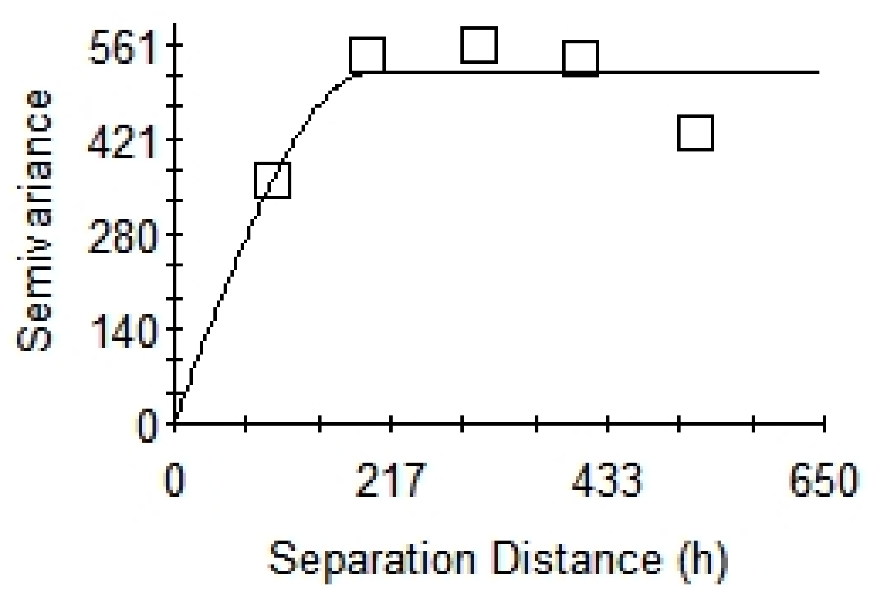
The AWHC data based on different sampling depths were combined together to obtain total AWHC values of up to 90 cm. Then, these data were summarized according to location (longitude and latitude) in an excel file. After this, the data were imported into GS+ Software Version 7.0, Gamma Design Software, LLC, Michigan, USA for analysis and to produce a best-fitted semivariogram to assess the spatial function. Values for the active lag distance and lag class distance interval were manually inserted. The procedures started with calculation of the semivariance based on a maximum lag distance of 650 m, which was divided into five lag distance classes separated by an average of 120 m. There were at least 38–120 pairs of points for each lag distance and most distance classes contained at least 38 pairs of data points. The best model for the variogram was selected based on visual fit and the highest R2 value of the model trendline. Later on, all variables used in GS+ software were utilized in ArcGIS 10.3, Esri Inc, California, USA software in order to make an interpolation map. Finally, data for each IMZ were analyzed using one-way ANOVA and the Tukey–Kramer test using SAS Software Version 9.4, SAS Institute Inc., Cary, NC, USA.
2.6. Irrigation Requirement Simulation Using FAO Cropwat Version 8.0
The FAO Cropwat model was developed by FAO to estimate crop water requirements (CWR), especially for food crops. This computer programme allows the development of irrigation schedules covering different management options, as well as the calculation of water supply schemes for varying crop patterns. The data from Section 2.3 were inserted into this software according to its modules. Generally, four modules were involved, which were the climate/ETo, rain, crop, and soil modules. For the climate module, yearly MnT, MxT, RH, WS, and SH data were inserted into this software, then later the monthly ETo data were generated based on the Penman–Montieth equation. Rainfall data were inserted into the ‘rain’ module and the effective rainfall was calculated by selecting the FAO/AGLW formula. For the ‘crop’ module, the planting date was set at the beginning of the year and the harvest date was set at the end of the year, without any crop stage. This was due to the oil palm crop being categorized as perennial and the observation period being a yearly assessment. The Kc value was set as 0.8 for the entire year, while the rooting depth was set as 0.60 m. In the ‘soil’ module, the average AWHC values from Section 2.5 were inserted into the ‘total available soil moisture’ section according to each zone assessment. The initial soil moisture depletion level was set at 100% to assume that the initial soil was dry at the early stage for maximum estimation of the water requirements. This software automatically calculated the TNI (Equation (4)) derived from the field balance equation. In Equation (4) [24], IRn is the net irrigation requirement (mm), ETc is crop evapotranspiration (mm), Pe is the effective dependable rainfall (mm), Ge is the groundwater contribution from the water table (mm), Wb is the water stored in the soil at the beginning of each period (mm), and LRmm is the leaching requirement (mm).
IRn = ETc − (Pe + Ge + Wb) + LRmm
3. Results and Discussion
3.1. Water Usage
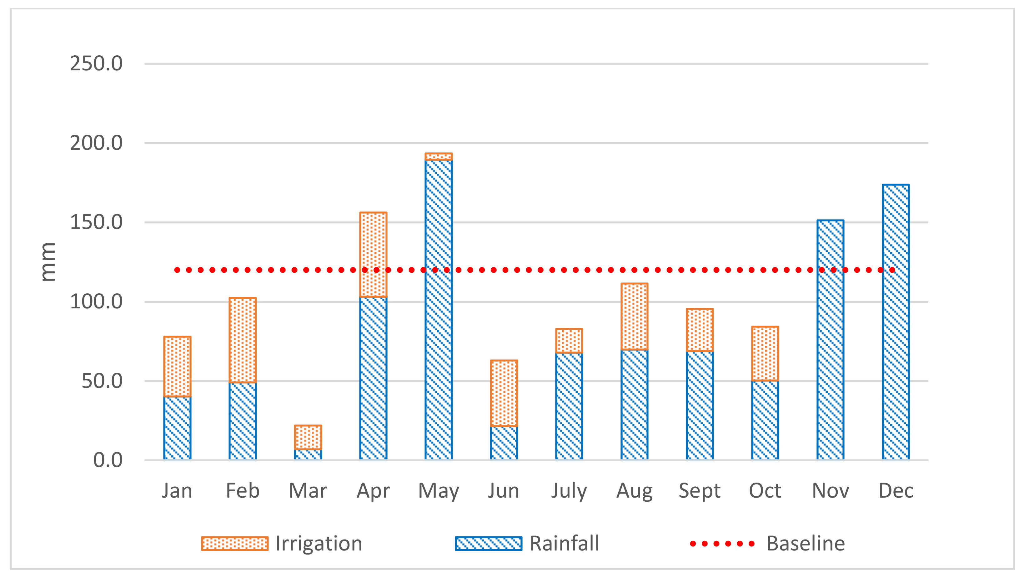
The study area received low rainfall for the year 2016, which was only 992 mm/year−1, with eight months receiving rainfall below 100 mm/month−1. The highest EID values were in February and April, which equaled 86 mm month−1, whilst the lowest was in May, which only 6.0 mm month−1. There were no irrigation events from November to December because of the sufficient rain on top of the monsoonal periods at this time (Figure 3); however, the EVW in March was very low, even though there was a low amount of rainfall. The number of rainy days can indicate the total solar radiation and potential crop evapotranspiration (ETc); hence, a red dotted line was used at 120 mm as a baseline, which represented the minimum value for ETc suggested by IRHO [25]. In Mac, the total water availability was only 21.9 mm month−1, which deviated by 82% from the baseline. In this case, the EID was limited to only 15.1 mm, which was explained by the scarcity of water, including the main source from the river. The river water level was too low below the drawing point, meaning irrigation was impossible. The issue of limited water sources can be considered as a determinant factor for irrigation implementation. The decision to source other water sources such as ground water can incur high costs and can require further studies.
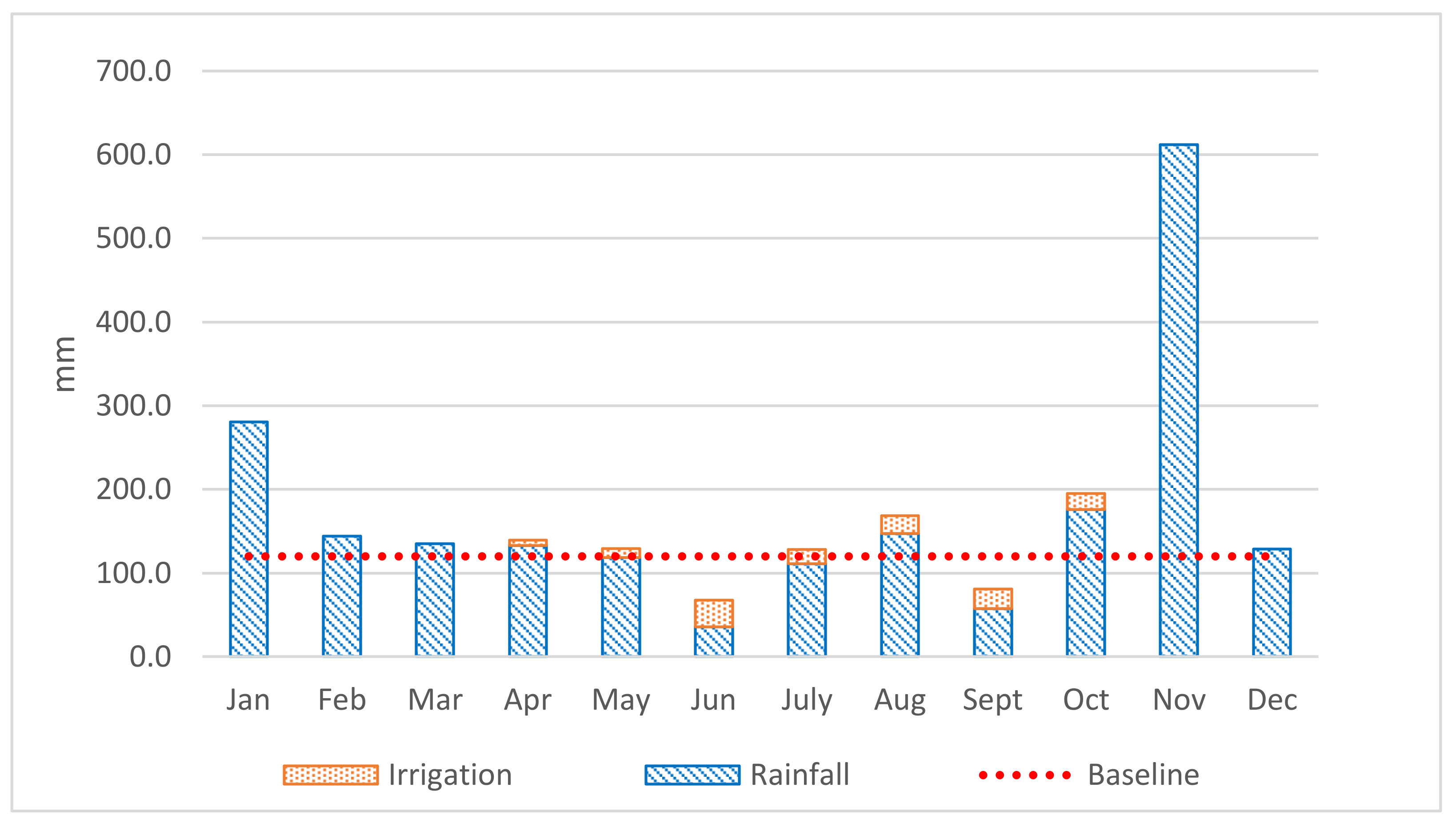
The year 2016 was the warmest year for Malaysia, which was strongly influenced by the super El Niño weather system that occurred until the middle of the year [26]. The opposite trend occurred for the year 2017, when the rainfall distribution was quite good at up to 2083 mm for the year. During this year, no irrigation occurred from January to March and for November to December (Figure 4). In fact, the rainfall amount in November was as high as 600 mm month−1. The gap between the water deficits (June and September) was much closer to the baseline. Based on [27], the El Niño Southern Oscillation (ENSO) index was neutral starting from January 2017 until the end of November 2017, followed by a weak La Niña condition starting in December 2017; thus, Malaysia did not experience long-lasting hot and dry weather throughout 2017.
3.2. Meteorological Data
The average values for the years 2016 and 2017 for the six main parameters are shown in Table 1. The lowest MnT ever recorded was 21.8 °C, while the highest temperature was 35.7 °C. High temperatures speed up moisture losses through evaporation and transpiration. In terms of RH, the readings were as 86.3%, which is normal for tropical regions. The relative humidity and temperature mainly affect the vapor pressure deficit. A relative humidity of 58% at 30 °C is equivalent to an increase of vapor pressure deficit above 1.8 kPa, which may close the stomata and reduce photosynthetic activity [28]. Apart from this, the WS values were similar for both years. As shown in Table 1, the monthly SH values were similar for both years, since the data originated from one source. This was an exceptional case due to the data being provided by FAO Climwat, which was not time-specified. There are technical difficulties, costs, and maintenance aspects associated with estate management related to obtaining complete climatic data, except for rainfall data; hence, FAO Climwat is an effortless solution for accessing data, while at the same time providing rational results for FAO Cropwat simulations [29]. Another advantage of this software is that it contains 15 years of data covering almost 5000 stations around the world [30]. All of these data points are important for the basic calculation or estimation of reference evapotranspiration (ETo) in FAO Cropwat.
3.3. Soil Data
Table 2 displays the matrix correlation between the AWHC and analyzed soil variables. A strong negative relationship was found between fine sand (FS) and clay particles (r < −0.80). This indicates that one variable is inferior while the other one is dominant. FS was found to be negatively correlated with soil depth and had a high percentage of 82–83% of total sand (TS), meaning it dominated with a higher r2 (0.93) compared to the coarse sand (CS). AWHC is referred to as the capability of soil to retain water and is related to the total pore space. A higher pore space generally holds more water. This is aligned with the positive relationship between soil depth and clay particles. Clay, which is known to have smallest particle size in soil, has a much higher total pore space than other particles.
For this analysis, BD had a weak positive relationship with clay and a negative relationship with sand, although it proved to be statistically significant. This relationship might be due to the fact that lower porosity, for example in sandy soil, will result in higher bulk density compared to clay particles, which have higher total porosity. In addition, organic matter (OM) was moderately negatively correlated with soil depth. There was high OM at the upper part of the soil, since there was a lot of plant debris and other organic matter, while most of the OM remained at the top of soil and only a small fraction entered the soil bodies. OM is accepted worldwide as factor that can be used to improve the soil water-holding capacity; however, a strong positive relationship between OM and AWHC was not shown here, and in fact a negative correlation was observed. A previous study [31] proved that the ability of OM to improve available water capacity is very limited or overestimated.; any increases are more pronounce in sandy soil, followed by loam and clays. As such, this contradictory agreement can be explained by the decreasing OM availability over soil depth, which is compounded by the distribution of clay particles.
Note: * is for p values < 0.05, ** is for p values <0.01.
3.4. Irrigation Management Zone
The best fitting model for this data was the spherical isotropic variogram, with a range of 196 m and an acceptable R2 value of 0.645. The isotropic variogram showed that the spatial structure of the variables was consistent in all directions. The AWHC data were considered as strongly spatially dependent, as the nugget semivariance percentage was 0.19%, falling well below 25% [32]. The effective range was 196 m, confirming that the 100 m grid point was acceptable (Figure 5).
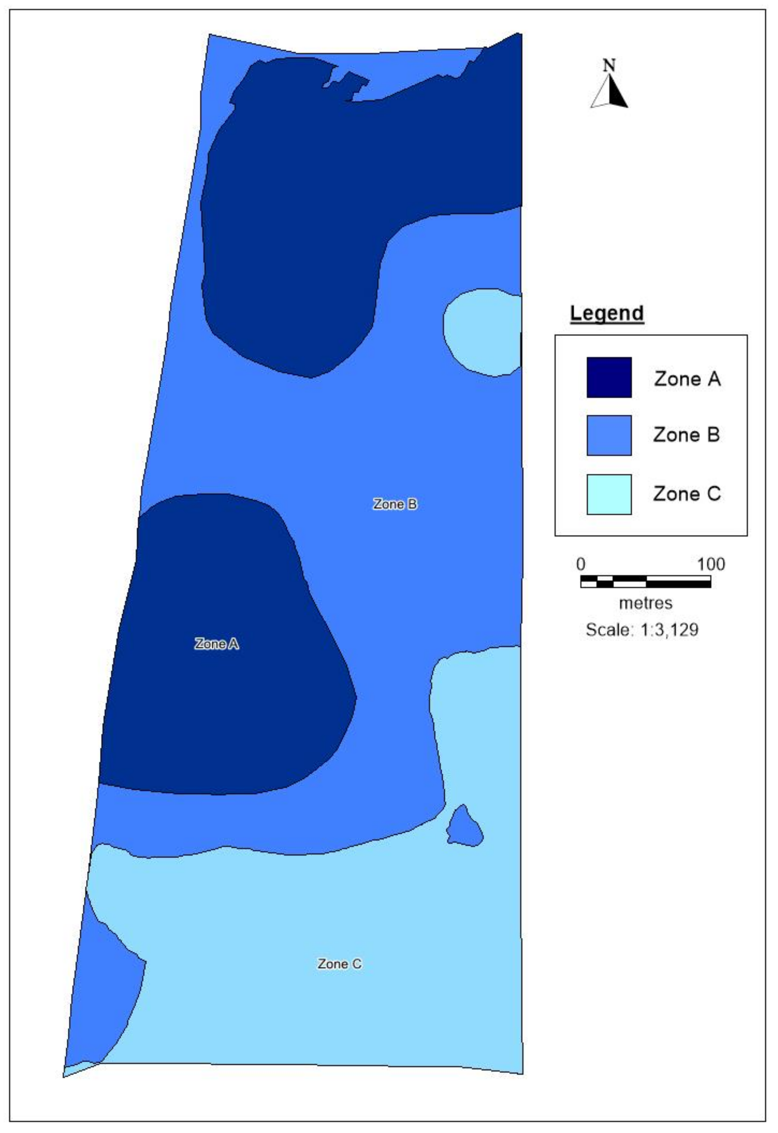
Generally, ArcGIS Software produced maps with a range of classifications according to different color schemes based on natural break classification modules. There are no clear guidelines for the number of classes that should be assigned; however, it is advised not to exceed seven classes [33]. In order to make things more reliable, three classifications were performed to divide the area into zones A, B, and C (Figure 6). A total 9 sampling points fell under zone A, 12 under zone B, and 7 under zone C. Based on one-way ANOVA and the Tukey–Kramer test, it was shown that each zone was highly significant to the others (Table 3). The selection of three zones was also based on a reliable and practical perspective of a precision operation system that will be installed in the future. The increasing number of management zones also resulted in higher installation costs due to the control and automation requirements. Through this study, it was found that soil can be classified into three different categories, although all soil are under the same soil series. Sometimes, delineation of IMZ values can provide more sophisticated and advanced data. Previous studies have shown that IMZ values can be delineated using Sentinel-2 images or field property data [34,35]. As in this study, IMZ values based on AWHC data are considered stable, and as a result can be used for many years as initial guidelines for growers or irrigation planners; however, the produced IMZ maps cannot be used to provide real-time soil moisture status information.
3.5. Crop Water Requirement (CWR)
This estate is located a dry region with average annual rainfall ranging from 1300 to 1800 mm per year. Based on the simulation, the CWR, which encompassed the total amount of water evapotranspirated, was 666.8 mm in 2016 and only 260.2 mm in 2017 (Table 4); however, these values were solely based on rainfall, without taking into consideration the soil water balance factor.
3.6. Comparison between TNI and EID for Each IMZ
Based on the soil sampling, this field was divided into three management zones called zones A, B, and C, each of which had a different AWHC range. The different AWHC values meant the water-holding capacity levels varied, affecting the irrigation timing. By taking into account the soil water capacity as a factor, the irrigation range in 2016 was below TNI level, ranging from 106 to 110 mm (Table 5). The insufficient EID values were partly due to the limited water sources, as mentioned before. Irrigation scheduling for rainfall amounts such as those in this study should probably follow the basic guidelines for palm crops. A water balance approach can be used to keep track of the soil water deficit by accounting for all water additions and subtractions from the soil root zone [36]. Furthermore, many types of soil moisture sensors can provide real-time and continuous data [37,38,39], improving the water use efficiency. Increasing the scheduling efficiency provides the opportunity to conserve water resources [40]. The EID value for 2017 was 130 mm, although the maximum TNI was only 96 mm. The surplus EID values ranged from 34 to 62 mm. Overirrigation means that extra energy resources will be required, such as gasoline, human resources, and maintenance costs. This also results in nitrogen leaching and runoff, increases in weed pressure, and disease, impeding growth and yield [41].
4. Conclusions
For many years, oil palm estates have been treated homogenously and the irrigation scheduling has been based on rainfall availability. As shown by geostatistical analysis, soil types can vary spatially, even though they are classified under the same soil series and can be treated as IMZs. It was found that clay, sand, and OM distributions varied with soil depth; however, no strong correlation was found between soil variables and AWHC. The rainfall distribution in 2016 was very low, which resulted in high CWR values compared to 2017. The EID value for 2016 of 322 mm year−1 was below requirements and contradicted the EID values for 2017, which surplus from 34 to 62 mm. Effective rainfall, soil, meteorological, and crop type data are very important in order to calculate the amount of water to be used for irrigation. The FAO Cropwat model can be a useful tool for estimating CWR values for an intended area, helping with decisions related to irrigation projects, giving a better understanding of and strong justification for such projects. In the future, sensor-based irrigation scheduling will be adopted and potential water savings resulting from the adaptation of precision irrigation in the field will be achieved.
Author Contributions
Conceptualization: A.W., Y.A.K., A.F.A. and M.R.M.; methodology: M.S.N., A.W., Y.A.K., A.F.A. and M.R.M.; investigation: M.S.N. and A.W.; writing—original draft preparation: M.S.N.; writing—review and editing: M.S.N.; supervision: A.W. All authors have read and agreed to the published version of the manuscript.
Funding
This research was funded by FGV Agri Services Sdn Bhd (FGVAS) for the project number FR-0604-27-0218 under the Collaborative Research and Development Agreement (CRDA) between FGV R&D Sdn Bhd and Universiti Putra Malaysia (UPM).
Institutional Review Board Statement
Not applicable.
Informed Consent Statement
Not applicable.
Data Availability Statement
FAO Climwat 2.0 Database software used in this project freely available and can be download at http://www.fao.org/land-water/databases-and-software/climwat-for-cropwat/en/.
Acknowledgments
We are grateful to the FGVAS Serting Estate manager, supervisors, and other staff for their information, co-operation, and help in conducting this study. We thank Khalifah Khalid and other Agronomy Department staff for taking soil samples and conducting the field work. We acknowledge Noor Hisham Hamid for their permission to publish this paper.
Conflicts of Interest
The authors declare no conflict of interest.
References
- Igor, A.S. World fresh water resources. In Water in Crisis: A Guide to the World’s Fresh Water Resources; Peter, H.G., Ed.; Oxford University Press: New York, NY, USA, 1993; pp. 13–24. [Google Scholar]
- UNFPA Annual Report 2020. Available online: https://www.unfpa.org/data/world-population-dashboard (accessed on 15 June 2021).
- Boretti, A.; Rosa, L. Reassessing the projections of the world water development report. NPJ Clean Water 2019, 2, 15. [Google Scholar] [CrossRef]
- Burek, P.; Satoh, Y.; Fisher, G.; Kahil, T.; Jimenez, L.N.; Scherzer, A.; Tramberend, S.; Wada, Y.; Eisner, S.; Florke, M.; et al. Water Futures and Solution, Fast Track Initiative; Working Paper, WP-16-006, Final Report; International Institute for Applied Systems Analysis (IIASA): Laxenburg, Austria, 2016. [Google Scholar]
- Ding, Y.; Tang, D.; Dai, H.; Wei, Y. Human-water harmony index: A new approach to assess the human water relationship. Water Resour. Manag. 2014, 28, 1061–1077. [Google Scholar] [CrossRef]
- Valipour, M.; Bateni, S.M.; Jun, C. Global surface temperature: A new insight. Climate 2021, 9, 81. [Google Scholar] [CrossRef]
- Wrachien, D.D.; Mudlagiri, B.G. Global Warming Impacts on Agriculture and Irrigation and Drainage Development. J. Agric. Aquac. 2019. Available online: https://escientificpublishers.com/global-warming-impacts-on-agriculture-and-irrigation-and-drainage-development-JAA-01-0007 (accessed on 13 July 2021).
- Harun, S.N.; Hanafiah, M.M. Estimating the country-level water consumption footprint of selected crop production. Appl. Ecol. Environ. Res. 2018, 16, 5381–5403. [Google Scholar] [CrossRef]
- Shahrizaila, A. Water Resource Users in Malaysia, Issues and Challenges. In Proceedings of the Malaysia Water Resources Management Forum. “Time for the Solution”, Perbadanan, Putrajaya, Malaysia, 26–27 November 2012. [Google Scholar]
- Zuraini, A.; Jaharudin, P.; Noorhaslinda, K.A.R.; Roseliza, M.A.; Haslina, M. Factors affecting water demand: Macro evidence in Malaysia. Jurnal Ekonomi Malaysia 2019, 53, 17–25. [Google Scholar]
- Department of Statistic Malaysia. Selected agriculture indicator. 2020. Available online: https://www.dosm.gov.my (accessed on 15 June 2021).
- Statista. Available online: https://www.statista.com/statistics/274127/world-palm-oil-usage-distribution/ (accessed on 15 June 2021).
- Lee, C.T.; Izwanizam, A. Lysimeter Studies and Irrigation of Oil Palm in Some Inland Soils of Peninsular Malaysia: Felda’s Experience. Planter 2013, 89, 15–29. [Google Scholar]
- Shahkhirat, M.N.; Umar, M.U.M.J.; Izwanizam, A.; Romzi, I.; Suhaidi, H. An Overview of Irrigation Approaches Implemented FELDA. In Proceedings of the 4th National Seminar on Oil Palm Mechanisation, Bangi, Malaysia, 23–24 October 2012. [Google Scholar]
- Mungkalasiri, J.; Wisansuwannakorn, R.; Paengjuntuek, W. Water footprint evaluation of oil palm fresh fruit bunches in Pathumthani and Chonburi, Thailand. Int. J. Environ. Sci. Dev. 2015, 6, 455–459. [Google Scholar] [CrossRef] [Green Version]
- Roundtable on Sustainable Palm Oil (RSPO). Principles and Criteria: For the Production of Sustainable Palm Oil. Revised 01 February 2020 with Updated Supply Chain Requirement for Mills. 56. Available online: https://www.rspo.org/resources/archive/1079 (accessed on 15 June 2021).
- Zulkifli, H.; Halimah, M.; Vijaya, S.; Choo, Y.M. Water footprint: Part 2, FFB production for oil palm planted in Malaysia. J. Oil Palm Res. 2014, 26, 282–291. [Google Scholar]
- Muaz, M.A.; Marlia, M.H. Water footprint assessment of oil palm in Malaysia: A preliminary study. AIP Conf. Proc. 2014, 1614, 803. [Google Scholar] [CrossRef]
- Bahagian Pengurusan dan Pemuliharaan Sumber Tanah. Panduan Mengenali Siri-Siri Tanah di Semenanjung Malaysia, 2nd ed.; Jabatan Pertanian: Kuala Lumpur, Malaysia, 2008; p. 75.
- Roslan, M.M.N.; Haniff, M.H. Water Deficit and Irrigation in Oil Palm: A Review of Recent Studies and Findings. Oil Palm Bull. 2004, 49, 1–6. [Google Scholar]
- FGVAS. Panduan 1; FGV Agri Services Sdn Bhd: Pahang, Malaysia, 2010; p. 122. [Google Scholar]
- Richards, L.A. Pressure Membrane Apparatus Construction and Use. Agric. Eng. 1947, 28, 451–454. [Google Scholar]
- Teh, B.S.C.; Jamal, T. Water Retention. In Soil Physics Analyses: Volume 1; Teh, B.S.C., Jamal, T., Eds.; University Putra Malaysia Press: Serdang, Malaysia, 2006; pp. 14–17. [Google Scholar]
- FAO. Crop Water Requirements and Irrigation Scheduling. In FAO Irrigation Manual Module 4; Savva, A.P., Frenken, K., Eds.; FAO: Rome, Italy, 2002; Available online: http://www.fao.org/3/ai593e/ai593e.pdf (accessed on 15 June 2021).
- Surre, C. Les Besoins en eau du palmier à huile: Calcul du Bilan de l’eau et ses Applications Pratiques. Oléagineux 1968, 23, 165–167. [Google Scholar]
- Malaysia Meteorological Department Annual Report. 2016. Available online: https://www.met.gov.my/content/pdf/penerbitan/laporantahunan/laporantahunan2016.pdf (accessed on 15 June 2021).
- Malaysia Meteorological Department Annual Report. 2017. Available online: https://www.met.gov.my/content/pdf/penerbitan/laporantahunan/laporantahunan2017.pdf (accessed on 15 June 2021).
- Jacquemard, J.C. Oil Palm: The Tropical Agriculturist; MacMillan Education Ltd.: Hong Kong, China, 1998; pp. 23–25. [Google Scholar]
- Shahkhirat, M.N.; Aimrun, W.; Yahya, A.K.; Fikri, A.A.; Razif, M.M. Quantitative Approach for Irrigation Requirement of Oil Palm: Case Study in Chuping, Northern Malaysia. J. Oil Palm Res. 2020, 33, 277–288. [Google Scholar] [CrossRef]
- FAO. Available online: http://www.fao.org/land-water/databases%20and-software/climwat-for-cropwat/en/ (accessed on 15 June 2021).
- Minasny, B.; McBratney, A.B. Limited effect of organic matter on soil available water capacity. Eur. J. Soil Sci. 2018, 69, 39–47. [Google Scholar] [CrossRef] [Green Version]
- Cambardella, C.A.; Moorman, T.B.; Novak, J.M.; Parkin, T.B.; Karlen, D.L.; Turco, R.F.; Konopka, A.E. Field-scale variability of soil properties in central Iowa soils. Soil Sci. Am. J. 1994, 58, 1501–1511. [Google Scholar] [CrossRef]
- Souza, E.G.; Schenatto, K.; Bazzi, C.L. Creating thematic maps and management zones for agriculture fields. In Proceedings of the 14th International Conference on Precision Agriculture, Montreal, QC, Canada, 24–27 June 2018; pp. 1–17. [Google Scholar]
- Liakos, V.; Vellidis, G.; Lacerda, L.; Tucker, M.; Porter, W.; Cox, C. Management Zone Delineation for Irrigation Based on Sentinel-2 Satellite Images and Field Properties. In Proceedings of the 14th International Conference on Precision Agriculture, Montreal, QC, Canada, 24–27 June 2018; pp. 1–11. [Google Scholar]
- Oldoni, H.; Bassoi, L.H. Delineation of irrigation management zones in a Quartzipsamment of the Brazilian semiarid region. Pesqui. Agropecu. Bras. 2016, 51, 1283–1294. [Google Scholar] [CrossRef] [Green Version]
- Andales, A.A.; Chávez, J.L.; Bauder, T.A. Irrigation Scheduling: The Water Balance Approach. Extension Fact Sheet, Colorado State University. 2011; p. 4. Available online: https://extension.colostate.edu/topic-areas/agriculture/irrigation-scheduling-the-water-balance-approach-4-707/ (accessed on 15 June 2021).
- Ruixiu, S. Irrigation Scheduling Using Soil Moisture Sensors. J. Agric. Sci. 2017, 10, 1–11. [Google Scholar] [CrossRef]
- Bittelli, M. Measuring soil water content: A review. HortTechnology 2011, 21, 293–300. [Google Scholar] [CrossRef]
- Evett, S.R.; Schwartz, R.C.; Tolk, J.A.; Howell, T.A. Soil profile water content determination: Spatiotemporal variability of electromagnetic and neutron probe sensors. Vadose Zone J. 2009, 8, 926–941. [Google Scholar] [CrossRef]
- McCready, M.S.; Dukes, M.D. Landscape Irrigation Scheduling efficiency and adequacy by various control technologies. Agric. Water Manag. 2011, 98, 697–704. [Google Scholar] [CrossRef]
- Irmak, S.; Rathje, W.R. Plant Growth and Yield as Affected by Wet Soil Conditions Due to Flooding or Over-Irrigation. Neb Guide Extension 2008. Institute of Agriculture and Natural Resources, University of Nebraska-Lincoln. 2008. Available online: https://extensionpublications.unl.edu/assets/pdf/g1904.pdf (accessed on 15 June 2021).
Figure 1.
Location of irrigation project in the study area.

Figure 2.
Google Earth map illustration showing the locations of detailed meteorological data collection sites. Sources used to estimate field data.
Figure 2.
Google Earth map illustration showing the locations of detailed meteorological data collection sites. Sources used to estimate field data.

Figure 3.
Monthly EID and rainfall distribution for FGVAS Serting Hilir Estate for 2016.

Figure 4.
Monthly EID and rainfall distribution for FGVAS Serting Hilir Estate in 2017.

Figure 5.
Semivariogram for AWHC data at FGVAS Serting Hilir Estate.

Figure 6.
Map of the irrigation management zones in the study site, named zone A, zone B, and zone C.
Figure 6.
Map of the irrigation management zones in the study site, named zone A, zone B, and zone C.


Table 1.
Summary of monthly meteorological data used in the FAO Cropwat model according to assessment year.
Table 1.
Summary of monthly meteorological data used in the FAO Cropwat model according to assessment year.
| Month | Rainfall | MnT | MxT | RH | WS | SH | Month | Rainfall | MnT | MxT | RH | WS | SH |
|---|---|---|---|---|---|---|---|---|---|---|---|---|---|
| mm | °C | °C | % | m/s | Hours | mm | °C | °C | % | m/s | Hours | ||
| 2016 | 2017 | ||||||||||||
| January | 40.1 | 23.8 | 33.0 | 81.9 | 1.5 | 5.7 | January | 281.1 | 23.1 | 31.3 | 85.2 | 1.1 | 5.7 |
| February | 49.2 | 23.3 | 32.2 | 81.9 | 1.8 | 6.5 | February | 144.3 | 22.6 | 31.4 | 84.0 | 1.1 | 6.5 |
| March | 6.8 | 24.2 | 35.0 | 75.4 | 1.5 | 6.8 | March | 135.6 | 23.4 | 32.6 | 82.5 | 1.0 | 6.8 |
| April | 103.2 | 24.6 | 35.7 | 76.4 | 1.2 | 6.7 | April | 133.1 | 23.8 | 33.0 | 84.0 | 0.8 | 6.7 |
| May | 189.6 | 24.4 | 34.0 | 83.6 | 1.0 | 6.6 | May | 118.8 | 23.9 | 32.3 | 81.5 | 1.1 | 6.6 |
| June | 21.4 | 23.1 | 32.1 | 83.5 | 1.0 | 6.4 | June | 35.9 | 23.2 | 32.4 | 80.2 | 1.1 | 6.4 |
| July | 67.8 | 22.7 | 32.7 | 82.2 | 1.1 | 6.3 | July | 111.7 | 23.0 | 32.0 | 78.2 | 1.3 | 6.3 |
| August | 69.8 | 23.3 | 33.2 | 78.2 | 1.3 | 6.1 | August | 147.6 | 23.1 | 31.5 | 80.7 | 1.1 | 6.1 |
| September | 68.9 | 23.2 | 33.3 | 79.8 | 1.2 | 5.7 | September | 57.7 | 23.3 | 32.0 | 80.8 | 1.1 | 5.7 |
| October | 50.3 | 23.4 | 33.1 | 77.9 | 1.3 | 5.6 | October | 176.5 | 23.4 | 32.5 | 82.0 | 0.9 | 5.6 |
| November | 151.4 | 22.2 | 30.6 | 86.3 | 1.0 | 5.1 | November | 612.5 | 23.3 | 31.0 | 85.6 | 0.9 | 5.1 |
| December | 173.9 | 21.8 | 30.5 | 85.2 | 1.1 | 4.9 | December | 129.1 | 23.4 | 31.2 | 83.3 | 1.1 | 4.9 |
Table 2.
Relationships between each of the soil variables with AWHC.
| Depth | AWHC | BD | Clay | Silt | CS | FS | TS | OM | OC | |
|---|---|---|---|---|---|---|---|---|---|---|
| Depth | 1 | |||||||||
| p-value | 0 | |||||||||
| AWHC | 0.5535 | 1 | ||||||||
| ** | 0 | |||||||||
| BD | −0.0525 | 0.0717 | 1 | |||||||
| 0.6439 | 0.5274 | 0 | ||||||||
| Clay | 0.5297 | 0.1371 | −0.3011 | 1 | ||||||
| ** | 0.2254 | ** | 0 | |||||||
| Silt | −0.048 | −0.2798 | −0.1618 | 0.2783 | 1 | |||||
| 0.6722 | * | 0.1515 | * | 0 | ||||||
| CS | −0.1169 | −0.1558 | 0.2407 | −0.4384 | −0.1925 | 1 | ||||
| 0.3016 | 0.1675 | * | ** | 0.0871 | 0 | |||||
| FS | −0.4021 | 0.0784 | 0.2519 | −0.8136 | −0.6495 | 0.0871 | 1 | |||
| ** | 0.4895 | * | ** | ** | 0.4421 | 0 | ||||
| TS | −0.4033 | 0.0109 | 0.3162 | −0.8926 | −0.6529 | 0.4571 | 0.9259 | 1 | ||
| ** | 0.9238 | ** | ** | ** | ** | ** | 0 | |||
| OM | −0.5564 | −0.3115 | −0.191 | −0.2966 | 0.0732 | −0.0526 | 0.2467 | 0.2003 | 1 | |
| ** | ** | 0.0897 | ** | 0.5189 | 0.6431 | * | 0.0748 | 0 | ||
| OC | −0.0425 | −0.0012 | −0.214 | 0.3197 | −0.0892 | −0.3296 | −0.1239 | −0.2356 | 0.194 | 1 |
| 0.7081 | 0.9916 | 0.0567 | ** | 0.4316 | ** | 0.2735 | * | 0.0847 | 0 |
Note: * is for p values < 0.05, ** is for p values < 0.01.
Table 3.
Management of zones for the three AWHC categories.
| Zone | AWHC (mm) | n | Mean | Grouping 1 | Hectares (ha) |
|---|---|---|---|---|---|
| A | 126 to 167 | 9 | 140 | a | 7.62 |
| B | 101 to 125 | 12 | 109 | b | 9.23 |
| C | 79 to 100 | 7 | 86 | c | 6.57 |
1 Different letters shown significant differences with p < 0.001.
Table 4.
CWR values for Serting Estate for 2016 and 2017.
| Year | Rainfall (mm) | CWR (mm) |
|---|---|---|
| 2016 | 992.4 | 666.8 |
| 2017 | 2083.4 | 260.2 |
Table 5.
The TNI and EID values for the years 2016 and 2017 according to the management zone.
| Year | 2016 | 2017 | ||||
|---|---|---|---|---|---|---|
| Zone | TNI (mm) | EID | Surplus (+) or Deficit (−) in mm | TNI (mm) | EID | Surplus (+) or Deficit (−) in mm |
| (mm Year−1) | (mm Year−1) | |||||
| A | 428 | 322 | –106 | 68 | 130 | 62 |
| B | 432 | 322 | –110 | 84 | 130 | 46 |
| C | 432 | 322 | –110 | 96 | 130 | 34 |
Note: The irrigation timing was set at 50% depletion of AWC and at a depth of 5 mm per irrigation event.
Publisher’s Note: MDPI stays neutral with regard to jurisdictional claims in published maps and institutional affiliations. |
© 2021 by the authors. Licensee MDPI, Basel, Switzerland. This article is an open access article distributed under the terms and conditions of the Creative Commons Attribution (CC BY) license (https://creativecommons.org/licenses/by/4.0/).
Share and Cite
MDPI and ACS Style
Norizan, M.S.; Wayayok, A.; Abdullah, A.F.; Mahadi, M.R.; Abd Karim, Y. Spatial Variations in Water-Holding Capacity as Evidence of the Need for Precision Irrigation. Water 2021, 13, 2208. https://doi.org/10.3390/w13162208
AMA Style
Norizan MS, Wayayok A, Abdullah AF, Mahadi MR, Abd Karim Y. Spatial Variations in Water-Holding Capacity as Evidence of the Need for Precision Irrigation. Water. 2021; 13(16):2208. https://doi.org/10.3390/w13162208
Chicago/Turabian StyleNorizan, Mohd Shahkhirat, Aimrun Wayayok, Ahmad Fikri Abdullah, Muhammad Razif Mahadi, and Yahya Abd Karim. 2021. "Spatial Variations in Water-Holding Capacity as Evidence of the Need for Precision Irrigation" Water 13, no. 16: 2208. https://doi.org/10.3390/w13162208
Note that from the first issue of 2016, this journal uses article numbers instead of page numbers. See further details here.