Optimization of Multi-Quality Water Networks: Can Simple Optimization Heuristics Compete with Nonlinear Solvers?

Abstract

Optimal management of water systems tends to be very complex, especially when water quality aspects are included. This paper addresses the management of multi-quality water networks over a fixed time horizon. The problem is formulated as an optimization program that minimizes cost by determining the optimal flow distribution that satisfies the water quantity and quality requirement in the demand nodes. The resulted model is nonlinear and non-convex due to bilinear terms in the mass balance equations of blending multi-quality flow. This results in several local optima, making the process of solving large-scale problems to global optimality very challenging. One classical approach to deal with this challenge is to use a multi-start procedure in which off-the-shelf local optimization solvers are initialized with several random initial points. Then the final optimal solution is considered as the lowest objective value over the different runs. This will lead to a cumbersome and slow solution process for large-scale problems. In light of the above, this study supports using ultra-fast simple optimization heuristics, which despite their moderate accuracy, can still reach the optimum solution when run many times using a multi-start procedure. As such, the final solution from simple optimization heuristics can compete with off-the-shelf nonlinear solvers in terms of accuracy and efficiency. The paper presents a simple optimization heuristic, which is specially tailored for the problem and compares its performance with a state-of-the-art nonlinear solver on large-scale systems.

1. Introduction

In recent years, water scarcity is being acknowledged across the world as an immediate threat to current and future sustainability. The threat is even more relevant in arid and semi-arid regions such as Middle East-North Africa (MENA) region. The MENA region is considered one of the most water-scarce regions in the world [1]. Thus, efficient planning and management for the water resources systems are crucial. Optimization models for water systems planning and management are considered an effective tool to aid in the decision-making process for managing water resources and their related infrastructure [2]. These models can be classified by the function they solve and the constraints they include. Simpler models only include quantity (Q) variables and only solve the quantitative aspect of the system. Some models are quantity-driven (with hydraulic considerations), called Q-H models. These models solve the problem with quantity variables while taking into account hydraulic consideration. When used in operational problems the Q-H models usually solve real-time systems with low temporal resolution such as hours or part of the hour [3]. Other models include the quality aspect of the water system, and these are called Q-C models. These models have two sets of decision variables (flow and concentration), but they do not include hydraulics explicitly. That is, they rely on the inherent assumption that the network is hydraulically feasible [4,5]. Additionally, some models deal with all three aspects; these are called Q-H-C models. Cohen et al. [6,7,8] developed an optimization model that consists of three separate models: a Quality-Quantity (Q-C) model, a Quantity-Hydraulic (Q-H) model, and a Quantity-Quality-Hydraulic (Q-C-H) model, which is a combination of the other two models.

Typically, early models for regional water supply systems management deal with quantities of water delivered from sources to demand zones. However, since over-pumping and exploitation of the sources have intensified natural processes of salinization and contamination, it became more important to include water quality aspects in the models [9,10,11,12]. Moreover, to meet the growing demands and to cope with water scarcity due to climate change, there is an increasing reliance on non-conventional water sources (e.g., reclaimed water, seawater desalination, brackish water) in integrated water supply systems [13,14]. As such, many water systems rely on a diversified portfolio of conventional and non-conventional water resources, which may have different qualities. This will necessitate the inclusion of water quality aspects since multi-quality water sources will be subject to blending in the conveyance network [15,16,17]. In these systems with multi-quality water sources, consumers will impose constraints on both water quantity and quality [18]. It is important to note that to account for sustainability goals, regional water supply systems models require a relatively long time horizon that assures adequate water sources in terms of both quality and quantity. In light of the above, there is a need for management models for Multi-year, Multi-quality Water Supply Systems (MMWSS).

Modeling the MMWSS problem will result in nonlinear and non-convex optimization models. This is because the quality (concentration) in the network edges, which is unknown, depends on the flow, which is also unknown, and on the quality of the water sources. Specifically, nonlinearity and non-convexity are due to the use of bilinear terms in the solute mass balance equations. For example, when salinity aspects are introduced, the mathematical model turns nonlinear due to the bilinear equation of salt mass balance in each mixing junction of the conveyance network. That is, to calculate the mass of salt in a junction, the concentration variables have to be multiplied by the flow variables causing the bilinear system of equations [16,17]. These characteristics of nonlinearity and non-convexity introduce several local optima, making the process of solving large-scale problems to global optimality very challenging [19]. Therefore, developing efficient solution algorithms for large-scale MMWSS is very desirable.

In previous studies, such as [20,21,22,23], the quality variables were simulated outside the optimization program so that a simpler optimization problem is obtained. For example, in [23] an external module that consists of an Artificial Neural Network (ANN) is used to estimate the water quality in the system, while in [22] water quality requirements are represented by flow constraints. Cai et al., in [20], developed a multi-quality model for a river basin where salinity presents a major environmental problem. The model has a time horizon for a single year with monthly time steps. To deal with the complexity of the model, a decomposition approach was adapted. The model is broken up into four sub-problems; the first one is the flow balance with fixed salinity. The second is the first, plus salt mass balance. The third is the second, plus the relationships defining the effect of soil salinity on crop yield. The fourth problem is actually like the primary problem with no infeasibilities. Clearly, these approaches that do not simultaneously consider quality and quantity variables result in suboptimal solutions.

Other studies consider the joint optimization of quality and quantity of multi-quality water networks, but many of them were solved using local nonlinear solvers [4,6,16,17,24,25,26]. For example, [6] solved a model of a multi-quality water supply system that minimizes the cost of operation composed of several components: pumping from sources, transportation, treatment, and yield reduction cost depending on water quality. The model is nonlinear and non-convex and it was solved using a local solver based on the projected gradient method [27]. Ostfeld and Shamir, in [24], solved a model for the optimal operation policy of a multi-quality water supply system, which consists of the following elements: sources, reservoirs, pipes, pumping stations, treatment plants, and consumption nodes. The objective function was to minimize the total operational cost. The solution was obtained using a local solver of GAMS/MINOS [28]. In a later study, Ostfeld and Shamir [25] developed an integrated model for joint design and management of multi-quality water supply systems. Due to non-smoothness, the r-algorithm [29] was adapted to solve the optimization problem. Zaide [4] solved the MMWSS problem by nonlinear optimization solver using the Generalized Reduced Gradient (GRG) algorithm [30]. The author notes that using this direct approach is limited to small or mid-scale problems. As such, to deal with the large size of the problem, [4] performed a relaxation in the model to reduce its size. It is obvious that this kind of relaxation will often lead to a suboptimal solution for the problem. As opposed to [4], [16] suggested a different reduction scheme that does not change the original model. In [16] all the salinity variables are eliminated using algebraic manipulations such that a smaller optimization problem was obtained. The reduced problem is then solved using a local nonlinear optimization solver which is based on the Interior-Point algorithm [31]. While this reduction scheme is good in reducing the model size (i.e., number of decision variables), it was found to introduce more nonlinearity in the model. Thus, the nonlinear solver might converge to a locally optimal solution.

The studies in [5,32] followed a different approach in which computationally expensive search methods such as Genetic Algorithms are used to solve the nonlinear non-convex mathematical model. In [5] a quality-quantity flow model to optimize water distribution in a regional water supply system with multi-quality sources is developed. The model is a nonlinear optimization model with monthly operation units and a six-month management horizon. The nonlinear mathematical model is solved by a hybrid Genetic Algorithm (GA), in which a GRG algorithm is embedded in the GA to optimize the objective function for each fitness evaluation. Cai et al., [32] adopted a similar hybrid GA approach for solving large-scale nonlinear water management models. The proposed approach solves a linear program for each fitness evaluation. These hybrid approaches are computationally expensive, especially because an inner optimization problem must be solved for each fitness function evaluation of the search algorithm.

Solution efficiency and accuracy are crucial properties when solving MMWSS models. A local nonlinear solver may converge to different solutions depending on different initial points; this makes it untrusted for real-life decision-making. One classical approach to deal with this challenge is to use a multi-start procedure in which off-the-shelf local optimization solvers are initialized with several random initial points. Then the final optimal solution is considered as the lowest objective value over the different runs. However, this will lead to a cumbersome and slow solution process for large-scale problems, which prevents real-time interaction with the model results. Solution efficiency is a desired property for model users since it facilitates real-time discussion of the model’s results between multiple stakeholders.

In light of the above, this study supports using ultra-fast, simple optimization heuristics, which despite their moderate accuracy, can still reach the optimum solution when run many times using a multi-start procedure. Namely, since a multi-start procedure should be used for local solution approaches, it might be advantageous to use many fast trials of simple solvers as opposed to using sophisticated slow solvers that have a higher likelihood to reach good solutions. Running a large number of trials of simple local solvers can compensate for its moderate accuracy in reaching good solutions. As such, the final solution from simple optimization heuristics can compete with off-the-shelf nonlinear solvers in terms of accuracy and efficiency. The paper presents a simple optimization heuristic, which is specially tailored for the MMWSS problem, and compares its performance with a state-of-the-art nonlinear solver (IPOPT) on large-scale systems. IPOPT is an open-source nonlinear optimization solver, which uses the interior-point algorithm [31]. Our local optimization heuristic builds on tools of convex optimization to find local optima of the MMWSS problem. The solution approach leverages the ability to efficiently solve linear programs. It iterates between solving a linear program that approximates the original problem and solving a single variable nonlinear optimization problem that reduces the infeasibility of the linear approximation. This local heuristic depends on the initial point that is used to build the first linear approximation. It is therefore typical to initialize the algorithm with several randomly chosen initial points and take the final point as the one with the lowest objective value over the different runs.

The idea of using sequential convex sub-problems is not new. The famous Sequential Linear Programming (SLP) algorithm [33,34] and Sequential Quadratic Programming (SQP) algorithm [35], utilize this concept. However, these approaches require trust regions to ensure convergence and to limit the iterations to a region where the approximation is valid [36]. Unlike these procedures, our suggested heuristic does not require a trust region. In the suggested approach, the MMWSS problem characteristics are utilized to iterate between the linear approximations and a new (easy-to-solve) nonlinear problem that directs the solution process toward the feasible region of the original nonlinear optimization problem.

2. The Nonlinear MMWSS Formulation

The water network is comprised of a set of nodes that represent sources, mixing junctions and demand zones, and a set of links that represent the flow of water from one node to the other. Water flow and quality (concentration) in each link are modeled using mass balance equations in each node. For concentration in the links, we consider a nonreactive solute assuming complete mixing at the nodes. The objective is to select the optimal flow distribution in the network that minimizes the overall cost of the management horizon subject to bounding constraints on flow and concentration.

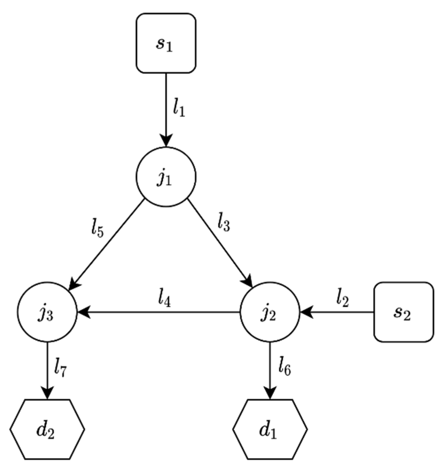
A water network with $j\in J$ mixing junctions and $l\in L$ links can be represented using nodes-links incidence matrix, $A\in R^{\left|J\right|\times \left|L\right|}$. The matrix has a row for each node and a column for each link such that the only nonzero elements in each row are $+1$ and $-1$ for incoming and outgoing links respectively. We also define the sources set $S$ with elements $\{s_1,\dots ,s_{\left|S\right|}\}$ and the demands set $D$ with elements $\{d_1,\dots ,d_{\left|D\right|}\}$. For example, the system in Figure 1, with two sources, two demand nodes, and three mixing junctions, has an incidence matrix $A\in R^{3\times 7}$ as given in

Table 1. Nodes-links incidence matrix, $A,$ for the illustrative example.

	l1	l2	l3	l4	l5	l6	l7
j1	+1	0	−1	0	−1	0	0
j2	0	+1	+1	−1	0	−1	0
j3	0	0	0	+1	+1	0	−1

and the sets $J=\{j_1,j_2,j_3\}$, $S=\{s_1,s_2\}$, $D=\{d_1,d_2\}$ and $L=\{l_1,\dots ,l_7\}$.

2.1. Objective Function

The objective function is to minimize the total operation cost. The cost is the sum of two different costs: conveyance cost and cost of water production in sources.

$$cost={\displaystyle \sum }_{t=1}^T\left(C{C}^t+P{C}^t\right)$$

(1)

where $cost$ is the total sum of operational costs; $C{C}^t$ is the conveyance cost of year $t$; $P{C}^t$ is the production cost of year $t$. $T$ is the number of years in the management horizon.

In this model, the per-unit cost of production is predetermined. Hence, the production cost is calculated as in Equation (2).

$$\begin{array}{l}P{C}^t={\displaystyle \sum _{s\in S}^{}P{C}_s^t}\\ P{C}_s^t=PUP{C}_s^t\cdot Q_s^t\end{array}$$

(2)

where $P{C}_s^t$ is the production cost of source $s$ at time $t$; $Q_s^t$ is water production in source $s$ at time $t$; $PUP{C}_s^t$ is the per-unit production cost for source $s$ at time $t$.

Generally, the conveyance cost in the pipes is derived from the head-loss, which is calculated by the nonlinear Hazen–Williams formula. Nevertheless, in regional water systems such as those considered herein, it is possible to use the Hazen–Williams formula to obtain an average constant per-unit conveyance cost. For example, this can be done by assuming a typical hydraulic gradient for the short-term operation in the distribution system of 1‰ as given in Equation (3).

$$\begin{array}{l}C{C}_{}^t={\displaystyle \sum _{p\in P}^{}C{C}_p^t}\\ C{C}_p^t=PUC{C}_p^t\cdot Q_p^t\\ PUC{C}_p^t=\frac{X_p^t\cdot KWH{C}^t}{w^t\cdot \eta }\\ X_p^t=0.001\cdot L_p\end{array}$$

(3)

where $C{C}_p^t$ is conveyance cost in pipe $p$; $PUC{C}_p^t$ is the per-unit conveyance cost in pipe $p$; $Q_p^t$ is flow in pipe $p$; $X_p^t$ is head-loss in pipe $p$; $w^t$ is the number of pumping hours; $\eta$ is the efficiency; $KWH{C}^t$ is the energy cost; $L_p$ is the length of pipe $p$; $P$ is a set of pipes with elements $\{p_1,\dots ,p_{\left|P\right|}\}$.

2.2. Constraints

2.2.1. Water Conservation Law

Given the representation of the network as a directed graph with nodes-links incidence matrix, $A$, the water balance for each time step, $t$, is imposed by the following linear equation system that ensures water conservation at the network nodes:

$$A\cdot Q^t=0\hspace{0.17em}\hspace{0.17em}\hspace{0.17em}\hspace{0.17em}\hspace{0.17em}\hspace{0.17em}\hspace{0.17em}\hspace{0.17em}\hspace{0.17em}\hspace{0.17em}\hspace{0.17em}\hspace{0.17em}\hspace{0.17em}\hspace{0.17em}\hspace{0.17em}\hspace{0.17em}\hspace{0.17em}\hspace{0.17em}\hspace{0.17em}\forall t=1...T$$

(4)

where $Q_{}^t\in R^{\left|L\right|\times 1}$ is a vector of flow decision variables in the network links. Since the demanded flow is known, the flow ingoing the demand nodes is also fixed. That is, given the values of the flow to demand zones $Q_d^t$  $\forall d\in D$, the following linear equality constraints should be imposed:

$$I_D\cdot Q^t=Q_D^t\hspace{0.17em}\hspace{0.17em}\hspace{0.17em}\hspace{0.17em}\hspace{0.17em}\hspace{0.17em}\hspace{0.17em}\hspace{0.17em}\hspace{0.17em}\hspace{0.17em}\hspace{0.17em}\hspace{0.17em}\hspace{0.17em}\hspace{0.17em}\hspace{0.17em}\hspace{0.17em}\hspace{0.17em}\hspace{0.17em}\hspace{0.17em}\forall t=1...T$$

(5)

where $I_D\in R^{\left|D\right|\times \left|L\right|}$ is a given incidence matrix that extracts the demands’ links from the vector $Q^t$, namely, each row in $I_D$ is corresponding to a demand node where each element in the row takes the value one if the link is associated with the demand node and zero otherwise. $Q_D^t\in R^{\left|D\right|\times 1}$ is a given vector that collects the known demands $Q_d^t$ $\forall d\in D$. For the illustrative example in Figure 1, the definition of the matrix $I_D$ is given in

Table 2. Demands-links incidence matrix, $I_D$, for the illustrative example.

	l1	l2	l3	l4	l5	l6	l7
d1	0	0	0	0	0	+1	0
d2	0	0	0	0	0	0	+1

.

2.2.2. The Solute Mass Conservation Law

For each time period, $t$, the following bilinear (i.e., nonlinear, non-convex) system of equations ensures solute mass conservation at network nodes:

$$\begin{array}{l}A\cdot M^t=0\hspace{0.17em}\hspace{0.17em}\hspace{0.17em}\hspace{0.17em}\hspace{0.17em}\hspace{0.17em}\hspace{0.17em}\hspace{0.17em}\hspace{0.17em}\hspace{0.17em}\hspace{0.17em}\hspace{0.17em}\hspace{0.17em}\hspace{0.17em}\hspace{0.17em}\hspace{0.17em}\hspace{0.17em}\hspace{0.17em}\hspace{0.17em}\hspace{0.17em}\hspace{0.17em}\hspace{0.17em}\hspace{0.17em}\hspace{0.17em}\hspace{0.17em}\hspace{0.17em}\hspace{0.17em}\hspace{0.17em}\forall t=1...T\\ M^t=Q^t\circ C^t\hspace{0.17em}\hspace{0.17em}\hspace{0.17em}\hspace{0.17em}\hspace{0.17em}\hspace{0.17em}\hspace{0.17em}\hspace{0.17em}\hspace{0.17em}\hspace{0.17em}\hspace{0.17em}\hspace{0.17em}\hspace{0.17em}\hspace{0.17em}\hspace{0.17em}\hspace{0.17em}\hspace{0.17em}\hspace{0.17em}\hspace{0.17em}\hspace{0.17em}\hspace{0.17em}\hspace{0.17em}\hspace{0.17em}\forall t=1...T\end{array}$$

(6)

where $C_{}^t\in R^{\left|L\right|\times 1}$ is a vector of concentration decision variables in the network links; $M_{}^t\in R^{\left|L\right|\times 1}$ is a vector of solute mass in the network links; $\circ$ is the Hadamard (i.e., element-wise) product between two vectors. This bilinear system of equations is the only source of nonlinearity and non-convexity in the MMWSS problem. Since the concentration of the sources is known, the concentration that outgoes source nodes is fixed. That is, given the values of the concentrations in the sources $C_s^t$  $\forall s\in S$, the following linear equality constraints should be imposed:

$$I_S\cdot C^t=C_S^t\hspace{0.17em}\hspace{0.17em}\hspace{0.17em}\hspace{0.17em}\hspace{0.17em}\hspace{0.17em}\hspace{0.17em}\hspace{0.17em}\hspace{0.17em}\hspace{0.17em}\hspace{0.17em}\hspace{0.17em}\hspace{0.17em}\forall t=1...T$$

(7)

where $I_S\in R^{\left|S\right|\times \left|L\right|}$ is a given incidence matrix which extracts the sources’ links from vector $C^t$, namely, each row in $I_S$ is corresponding to a source node where each element in the row takes the value one if the link is associated with the source node and zero otherwise. $C_S^t\in R^{\left|S\right|\times 1}$ is a given vector that collects the known concentrations $C_s^t$  $\forall s\in S$. For the illustrative example in Figure 1, the definition of the matrix $I_S$ is given in

Table 3. Sources-links incidence matrix, $I_S$, for the illustrative example.

	l1	l2	l3	l4	l5	l6	l7
$s_1$	1	0	0	0	0	0	0
$s_2$	0	1	0	0	0	0	0

.

2.2.3. Dilution Condition

The model assumes total mixing at all junction nodes, so the salinity in all links leaving a node is the same. This dilution condition is given by the linear system of equations as defined in Equation (8).

$$B\cdot C^t=0\hspace{0.17em}\hspace{0.17em}\hspace{0.17em}\hspace{0.17em}\hspace{0.17em}\hspace{0.17em}\hspace{0.17em}\hspace{0.17em}\hspace{0.17em}\hspace{0.17em}\hspace{0.17em}\hspace{0.17em}\forall t=1...T$$

(8)

where the matrix $B\in R^{(|L|-|J|-|S|)\times \left|L\right|}$ is defined such that each row indicates equal concentration for two outgoing links which share the same node; i.e., each row has only two non-zero elements $+1$ and $-1$; when three links leave the same node there are two rows, each with two non-zero elements $+1$ and $-1$. In the illustrative example (Figure 1), the matrix $B\in R^{2\times 7}$ is given in

Table 4. Dilution constraints matrix, $B$, for the illustrative example.

	l1	l2	l3	l4	l5	l6	l7
j1	0	0	+1	0	−1	0	0
j2	0	0	0	+1	0	−1	0

. The junction nodes $j_1,j_2$ have two outgoing links, therefore each of them contributes one row in the matrix $B$.

2.2.4. Conveyance Capacity Constraints

The model deals with the balance of water and solute mass and does not consider explicitly the hydraulic energy balance of the system. However, to prevent infeasibilities of hydraulic conditions, the flows in the pipes are limited by capacity constraints in Equation (9). The lower bound is set to $Q_{p,\min }^t$, which is larger or equal to zero since the flow direction in the pipes is fixed.

$$Q_{p,\min }^t\le Q_p^t\le Q_{p,\max }^t\hspace{0.17em}\hspace{0.17em}\hspace{0.17em}\hspace{0.17em}\hspace{0.17em}\hspace{0.17em}\hspace{0.17em}\forall p\in P\hspace{0.17em}\hspace{0.17em}\hspace{0.17em}\forall t=1...T\hspace{0.17em}$$

(9)

where $Q_{p,\min }^t$, $Q_{p,\max }^t$ are the minimum and the maximum flow in pipe $p$, respectively.

2.2.5. Production Capacity Constraints

In each source, there is a maximum physical capacity in each period (e.g., pumping station capacity) as well as multi-period (i.e., cumulative) water production capacity that represents the overall production in the management horizon (e.g., to accounting for sustainability aspects, which ensure that the source is not overexploited). These constraints are given in Equations (10) and (11), respectively. Note that the lower bound, $Q_{s,\min }^t$, should be set to a non-negative value.

$$Q_{s,\min }^t\le Q_s^t\le Q_{s,\max }^t\hspace{0.17em}\hspace{0.17em}\hspace{0.17em}\hspace{0.17em}\hspace{0.17em}\hspace{0.17em}\hspace{0.17em}\forall s\in S\hspace{0.17em}\hspace{0.17em}\hspace{0.17em}\forall t=1...T\hspace{0.17em}$$

(10)

$${\displaystyle \sum _{t=1}^T{Q}_s^t}\le Q_{s,\max }^{total}\hspace{0.17em}\hspace{0.17em}\hspace{0.17em}\hspace{0.17em}\hspace{0.17em}\hspace{0.17em}\hspace{0.17em}\forall s\in S\hspace{0.17em}$$

(11)

where $Q_{s,\min }^t$, $Q_{s,\max }^t$ are the minimum and the maximum flow from source $s$, respectively; $Q_{s,\max }^{total}$ is the total amount of water withdrawal from source $s$.

2.2.6. Concentration Constraints

Concentration requirements are imposed in demand nodes. As such the concentration of water that reaches the demand node should be within a prescribed minimum and maximum concentration as given in Equation (12). In case the demand node does not have concentration bounds, practical bounds could be added using the known concentration of the sources by setting $C_{d,min}^t=\underset{s\in S}{\min }\left(C_s^t\right)\hspace{0.17em}$ and $C_{d,\max }^t=\underset{s\in S}{\max }\left(C_s^t\right)$ $\hspace{0.17em}\forall d\in D\hspace{0.17em}$ $\forall t=1...T$.

$$C_{d,\min }^t\hspace{0.17em}\le C_d^t\le C_{d,\max }^t\hspace{0.17em}\hspace{0.17em}\hspace{0.17em}\hspace{0.17em}\hspace{0.17em}\hspace{0.17em}\hspace{0.17em}\forall d\in D\hspace{0.17em}\hspace{0.17em}\hspace{0.17em}\forall t=1...T\hspace{0.17em}$$

(12)

where $C_{d,\min }^t$, $C_{d,\max }^t$ are the minimum and the maximum concentration in demand node $d$, respectively. In the absence of concentration limits in pipes, one can define the following bounds:

$$\underset{s\in S}{\min }\left(C_s^t\right)\le C_p^t\le \underset{s\in S}{\max }\left(C_s^t\right)\hspace{0.17em}\hspace{0.17em}\hspace{0.17em}\hspace{0.17em}\hspace{0.17em}\hspace{0.17em}\hspace{0.17em}\forall p\in P\hspace{0.17em}\hspace{0.17em}\hspace{0.17em}\forall t=1...T\hspace{0.17em}$$

(13)

2.3. Optimization Problem

The overall optimization model is given in Equations (14)–(22), hereafter we will donate this model as the Q-C model. This optimization problem is a nonlinear and non-convex optimization program due to the use of bilinear terms in the third constraint. This formulation is given in terms of decision variables in the network links $Q^t,C_{}^t,M_{}^t\in R^{\left|L\right|\times 1}$.

$$\min \hspace{0.17em}\hspace{0.17em}{\displaystyle \sum _{t=1}^T{f}^t\cdot Q^t}$$

(14)

Subject to

$$A\cdot Q^t=0\hspace{0.17em}\hspace{0.17em}\hspace{0.17em}\hspace{0.17em}\hspace{0.17em}\hspace{0.17em}\hspace{0.17em}\hspace{0.17em}\hspace{0.17em}\hspace{0.17em}\hspace{0.17em}\hspace{0.17em}\hspace{0.17em}\hspace{0.17em}\hspace{0.17em}\hspace{0.17em}\hspace{0.17em}\hspace{0.17em}\hspace{0.17em}\hspace{0.17em}\hspace{0.17em}\hspace{0.17em}\hspace{0.17em}\hspace{0.17em}\hspace{0.17em}\hspace{0.17em}\hspace{0.17em}\hspace{0.17em}\hspace{0.17em}\hspace{0.17em}\forall t=1...T$$

(15)

$$\begin{array}{l}A\cdot M^t=0\hspace{0.17em}\hspace{0.17em}\hspace{0.17em}\hspace{0.17em}\hspace{0.17em}\hspace{0.17em}\hspace{0.17em}\hspace{0.17em}\hspace{0.17em}\hspace{0.17em}\hspace{0.17em}\hspace{0.17em}\hspace{0.17em}\hspace{0.17em}\hspace{0.17em}\hspace{0.17em}\hspace{0.17em}\hspace{0.17em}\hspace{0.17em}\hspace{0.17em}\hspace{0.17em}\hspace{0.17em}\hspace{0.17em}\hspace{0.17em}\hspace{0.17em}\hspace{0.17em}\hspace{0.17em}\hspace{0.17em}\forall t=1...T\\ M^t=Q^t\circ C^t\hspace{0.17em}\hspace{0.17em}\hspace{0.17em}\hspace{0.17em}\hspace{0.17em}\hspace{0.17em}\hspace{0.17em}\hspace{0.17em}\hspace{0.17em}\hspace{0.17em}\hspace{0.17em}\hspace{0.17em}\hspace{0.17em}\hspace{0.17em}\hspace{0.17em}\hspace{0.17em}\hspace{0.17em}\hspace{0.17em}\hspace{0.17em}\hspace{0.17em}\hspace{0.17em}\hspace{0.17em}\hspace{0.17em}\forall t=1...T\end{array}$$

(16)

$$B\cdot C^t=0\hspace{0.17em}\hspace{0.17em}\hspace{0.17em}\hspace{0.17em}\hspace{0.17em}\hspace{0.17em}\hspace{0.17em}\hspace{0.17em}\hspace{0.17em}\hspace{0.17em}\hspace{0.17em}\hspace{0.17em}\hspace{0.17em}\hspace{0.17em}\hspace{0.17em}\hspace{0.17em}\hspace{0.17em}\hspace{0.17em}\hspace{0.17em}\hspace{0.17em}\hspace{0.17em}\hspace{0.17em}\hspace{0.17em}\hspace{0.17em}\hspace{0.17em}\hspace{0.17em}\hspace{0.17em}\hspace{0.17em}\hspace{0.17em}\hspace{0.17em}\forall t=1...T$$

(17)

$$I_S\cdot C^t=C_S^t\hspace{0.17em}\hspace{0.17em}\hspace{0.17em}\hspace{0.17em}\hspace{0.17em}\hspace{0.17em}\hspace{0.17em}\hspace{0.17em}\hspace{0.17em}\hspace{0.17em}\hspace{0.17em}\hspace{0.17em}\hspace{0.17em}\hspace{0.17em}\hspace{0.17em}\hspace{0.17em}\hspace{0.17em}\hspace{0.17em}\hspace{0.17em}\hspace{0.17em}\hspace{0.17em}\hspace{0.17em}\hspace{0.17em}\hspace{0.17em}\hspace{0.17em}\hspace{0.17em}\forall t=1...T$$

(18)

$$I_D\cdot Q^t=Q_D^t\hspace{0.17em}\hspace{0.17em}\hspace{0.17em}\hspace{0.17em}\hspace{0.17em}\hspace{0.17em}\hspace{0.17em}\hspace{0.17em}\hspace{0.17em}\hspace{0.17em}\hspace{0.17em}\hspace{0.17em}\hspace{0.17em}\hspace{0.17em}\hspace{0.17em}\hspace{0.17em}\hspace{0.17em}\hspace{0.17em}\hspace{0.17em}\hspace{0.17em}\hspace{0.17em}\hspace{0.17em}\hspace{0.17em}\hspace{0.17em}\hspace{0.17em}\forall t=1...T$$

(19)

$$Q_{\min }^t\le Q^t\le Q_{\max }^t\hspace{0.17em}\hspace{0.17em}\hspace{0.17em}\hspace{0.17em}\hspace{0.17em}\hspace{0.17em}\hspace{0.17em}\hspace{0.17em}\hspace{0.17em}\hspace{0.17em}\hspace{0.17em}\hspace{0.17em}\hspace{0.17em}\hspace{0.17em}\hspace{0.17em}\hspace{0.17em}\forall t=1...T$$

(20)

$$C_{\min }^t\le C^t\le C_{\max }^t\hspace{0.17em}\hspace{0.17em}\hspace{0.17em}\hspace{0.17em}\hspace{0.17em}\hspace{0.17em}\hspace{0.17em}\hspace{0.17em}\hspace{0.17em}\hspace{0.17em}\hspace{0.17em}\hspace{0.17em}\hspace{0.17em}\hspace{0.17em}\hspace{0.17em}\hspace{0.17em}\forall t=1...T$$

(21)

$${\displaystyle \sum _{t=1}^T{I}_S\cdot Q^t}\le Q_{S,\max }^{total}$$

(22)

where $f^t\in R^{1\times \left|L\right|}$ is a given row vector that collects the per-unit costs from Equations (2) and (3); $Q_{\min }^t$, $Q_{\max }^t\in R^{1\times \left|L\right|}$ are column vectors that collect the flow bounds from Equations (9) and (10); $C_{\min }^t$, $C_{\max }^t\in R^{1\times \left|L\right|}$ are column vectors that collect the concentration bounds from Equations (12) and (13); $Q_{S,\max }^{total}\in R^{\left|S\right|\times 1}$ is a given vector that collects the values $Q_{s,\max }^{total}$  $\forall s\in S$.

3. Simple Optimization Heuristic

As discussed previously, the inclusion of both quantity and quality variables increases the computational complexity of mathematical models because of the nonlinear and non-convex relationships involved in the solute mass balance. This heightened complexity is dominant in large-scale and long-term models. In view of this, it is a necessity to develop efficient solution methods to solve Q-C models. In this section, we propose and examine the performance of a Simple Optimization Heuristic (SOH) to solve quantity-quality management models. The basic idea consists of replacing the bilinear terms with first-order Taylor approximation to obtain a search direction. Then, this direction is used to formulate a simple nonlinear problem in which the infeasibility of the solute mass balance is minimized. The process is reiterated by successively solving linear and nonlinear optimization problems until convergence is obtained.

We denote the convex (polyhedral) feasible region of the constrains in Equations (15), (17)–(22) as $ℱ$, hence, after substitution of $M^t$, the optimization problem could be written in compact forms as:

$$\min \hspace{0.17em}\hspace{0.17em}{\displaystyle \sum _{t=1}^T{f}^t\cdot Q^t}$$

(23)

Subject to

$$\left(Q^{\forall t},C^{\forall t}\right)\in ℱ$$

(24)

$$A\cdot (Q^t\circ C^t)=0\hspace{0.17em}\hspace{0.17em}\hspace{0.17em}\hspace{0.17em}\hspace{0.17em}\hspace{0.17em}\hspace{0.17em}\hspace{0.17em}\hspace{0.17em}\hspace{0.17em}\hspace{0.17em}\forall t=1...T$$

(25)

To perform the linearization, the formulation of the Q-C model in Equations (23)–(25) remains the same except for the second constraint, which is the source of the nonlinearity and non-convexity. Thus, the linear approximation of the Hadamard (i.e., element-wise) product between two vectors is obtained based on the first order, bi-dimensional Taylor approximation as shown in Equations (26).

$$Q^t\circ C^t\approx C_{}^{t,k}\circ Q^t+Q_{}^{t,k}\circ C^t-Q_{}^{t,k}\circ C_{}^{t,k}$$

(26)

where $Q^{t,k}$ and $C^{t,k}$ are the approximation points at iteration $k$.

Using this convex approximation, the sequential linear approximation subproblem for iteration $k$ can be formulated as:

$$\min \hspace{0.17em}\hspace{0.17em}{\displaystyle \sum _{t=1}^T{f}^t\cdot Q^t}$$

(27)

Subject to

$$\left(Q^{\forall t},C^{\forall t}\right)\in ℱ$$

(28)

$$A\cdot (C_{}^{t,k}\circ Q^t+Q_{}^{t,k}\circ C^t-Q_{}^{t,k}\circ C_{}^{t,k})=0\hspace{0.17em}\hspace{0.17em}\hspace{0.17em}\hspace{0.17em}\hspace{0.17em}\hspace{0.17em}\hspace{0.17em}\hspace{0.17em}\hspace{0.17em}\hspace{0.17em}\hspace{0.17em}\forall t=1...T$$

(29)

This linearization, however, introduces a convex approximation of the feasible region, which might be smaller than the original feasible region of the optimization problem in Equations (23)–(25). This can lead to infeasibility in the linear subproblems. This issue of infeasibility in the subproblems is also encountered in SQP and other iterative techniques [37,38]. To deal with the feasibility of subproblems, we propose the following relaxation that introduces one penalized artificial variable in Equations (30) and (32). Clearly, the relaxed problem is always feasible (when the original problem has a nonempty feasible region), and the artificial variable $v$ corresponds to the maximum deviation in Equation (29).

$$\min \hspace{0.17em}\hspace{0.17em}{\displaystyle \sum _{t=1}^T{f}^t\cdot Q^t}+\beta \cdot v$$

(30)

Subject to

$$\left(Q^{\forall t},C^{\forall t}\right)\in ℱ$$

(31)

$$-v\le A\cdot (C_{}^{t,k}\circ Q^t+Q_{}^{t,k}\circ C^t-Q_{}^{t,k}\circ C_{}^{t,k})\le v\hspace{0.17em}\hspace{0.17em}\hspace{0.17em}\hspace{0.17em}\hspace{0.17em}\hspace{0.17em}\hspace{0.17em}\hspace{0.17em}\hspace{0.17em}\hspace{0.17em}\hspace{0.17em}\forall t=1...T$$

(32)

where $\beta$ is a predetermined penalty parameter, and $v$ is an artificial variable that ensures the feasibility of the constraint in Equation (32).

For large values of $\beta$, when the feasible region is nonempty, the solutions to the relaxed problem are solutions to the linear approximation problem in Equations (27)–(29), and the optimal value of $v$ will be zero [39]. Nonetheless, the feasibility of the linear approximation does not guarantee the feasibility of the original nonlinear problem in Equations (23)–(25). To move to the feasible region of the original nonlinear problem, another subproblem that reduces the nonlinear infeasibility between iterations is solved. Given the current approximation points, ( $Q^{t,k}$, $C^{t,k}$), and given the current solution of the relaxed problem, denoted as ( $Q_{lin}^{t,k}$, $C_{lin}^{t,k}$), the following single variable nonlinear optimization problem should be solved:

$$\begin{array}{l}\underset{\alpha }{\min }\hspace{0.17em}\hspace{0.17em}{\displaystyle \sum _{t=1}^T{f}^t\cdot Q^t(\alpha )}+\beta \cdot \max \left(RelInf(\alpha )-\epsilon ,0\right)\\ \mathrm{Subject}\hspace{0.17em}\mathrm{to}\\ 0\le \alpha \le 1\end{array}$$

(33)

where $\epsilon$ is predefined small acceptable tolerance; $Q^t(\alpha )$ is a point on the search direction as defined in Equation (34); $RelInf(\alpha )$ is the relative infeasibility and it is defined in Equation (36).

$$Q^t(\alpha )=(1-\alpha )\cdot Q^{t,k}+\alpha \cdot Q_{lin}^{t,k}$$

(34)

$$C^t(\alpha )=(1-\alpha )\cdot C^{t,k}+\alpha \cdot C_{lin}^{t,k}$$

(35)

$$RelInf(\alpha )=\frac{\Vert \hspace{0.17em}\hspace{0.17em}{\left[A\cdot \left(Q^t(\alpha )\circ C^t(\alpha )\right)\right]}_{\forall t}\Vert }{\Vert \hspace{0.17em}\hspace{0.17em}{\left[Q^t(\alpha )\circ C^t(\alpha )\right]}_{\forall t}\Vert }$$

(36)

where $\Vert \hspace{0.17em}\hspace{0.17em}\cdot \hspace{0.17em}\hspace{0.17em}\Vert$ is the Euclidean norm and the notation ${\left[\hspace{0.17em}\cdot \hspace{0.17em}\right]}_{\forall t}$ indicates a vector the collects all vectors for each $t=1...T$.

The relative infeasibility is interpreted as the violation in the solute mass balance relative to the solute mass that flows in the network. The relative measure of violation is considered to account for the magnitude of the solute mass in the network nodes. Consider, for example, a node with one ingoing pipe and one outgoing pipe where the flow in the two pipes is 100 million cubic meters per year, the salinity in each pipe is 200 mg-CL per Liter, then a violation of 1 kg in salt mass is negligible compared to the total salt mass, which is $2\times {10}^7$ kg.

It is noteworthy that any solution of the nonlinear problem in Equation (33) will be feasible for the set of constraints in $ℱ$. This is because for $0\le \alpha \le 1$, the values of $Q^t(\alpha )$ and $C^t(\alpha )$ are convex combinations of feasible points as defined in Equations (34) and (35). In light of the above, the SOH algorithm is stated in Algorithm 1.

Algorithm 1 Simple Optimization Heuristic
Given:	Randomly generated initial point $(Q^{t,0}$$,C^{t,0}$$)$ large positive penalty parameter β; small positive tolerance $\epsilon$$; k=0$
Repeat
	1. Solve Linear Approximation. Set the value of ($Q_{lin}^{t,k}$$,C_{lin}^{t,k}$) to the solution of the optimization problem in Equations (30)–(32).
	2. Solve Nonlinear Problem. Set the value of ($Q^{t,k+1}$$,C^{t,k+1}$) to the solution of the optimization problem in Equation (33).
	3. Update Iteration. k = k + 1
Until	Stopping criterion is satisfied.

3.1. Initialize

The SOH above is a local optimization heuristic; as such, the final point found may depend on the initial starting point. Therefore, the algorithm is initialized with several random initial points, where the best run among all runs is taken as the solution to the optimization problem.

3.2. Solve Linear Approximation

The obtained approximation is a linear problem, which could be solved with any off-the-shelf optimization solver. In this study, we used CPLEX [40] as the linear programming solver.

3.3. Solve Nonlinear Problem

The obtained problem in this step is nonlinear non-convex, but it is easy to solve because it only involves a single variable, which is bounded between zero and one. It is possible to solve this problem by grid search in the variable bounds or using dedicated nonlinear single variable methods. For example, in this study, we used the MATLAB solver fminbnd, which implements the golden section method [41].

3.4. Stopping Criterion

One reasonable stopping criterion is that the distance (Euclidean norm) between two successive points during the iteration process is less than the tolerance. However, we found that the SOH might oscillate between two points, which are not necessarily successive. To prevent oscillation, the algorithm stops if the current solution is within relative distance $\epsilon$ from any previously obtained solution in the iteration process. This condition is defined in Equation (37).

$$stop=\{\begin{array}{c}1\hspace{0.17em}\hspace{0.17em}\hspace{0.17em}\hspace{0.17em}\hspace{0.17em}\hspace{0.17em}\hspace{0.17em}\hspace{0.17em}\hspace{0.17em}\hspace{0.17em}\hspace{0.17em}\hspace{0.17em}\hspace{0.17em}\hspace{0.17em}\hspace{0.17em}\hspace{0.17em}\hspace{0.17em}if\hspace{0.17em}\hspace{0.17em}\hspace{0.17em}\hspace{0.17em}\underset{j=1...k}{\min }\left(\frac{\Vert \hspace{0.17em}\hspace{0.17em}{\left[Q^{t,k+1}\right]}_{\forall t}-{\left[Q^{t,j}\right]}_{\forall t}\Vert }{\Vert \hspace{0.17em}\hspace{0.17em}{\left[Q^{t,j}\right]}_{\forall t}\Vert }\right)<\epsilon \hfill \\ 0\hspace{0.17em}\hspace{0.17em}\hspace{0.17em}\hspace{0.17em}\hspace{0.17em}\hspace{0.17em}\hspace{0.17em}\hspace{0.17em}\hspace{0.17em}\hspace{0.17em}\hspace{0.17em}\hspace{0.17em}\hspace{0.17em}\hspace{0.17em}\hspace{0.17em}\hspace{0.17em}\hspace{0.17em}Otherwise\hspace{0.17em}\hspace{0.17em}\hspace{0.17em}\hspace{0.17em}\hspace{0.17em}\hspace{0.17em}\hspace{0.17em}\hspace{0.17em}\hspace{0.17em}\hspace{0.17em}\hspace{0.17em}\hspace{0.17em}\hspace{0.17em}\hspace{0.17em}\hspace{0.17em}\hspace{0.17em}\hspace{0.17em}\hspace{0.17em}\hspace{0.17em}\hspace{0.17em}\hspace{0.17em}\hspace{0.17em}\hspace{0.17em}\hspace{0.17em}\hspace{0.17em}\hspace{0.17em}\hspace{0.17em}\hspace{0.17em}\hspace{0.17em}\hspace{0.17em}\hspace{0.17em}\hspace{0.17em}\hspace{0.17em}\hspace{0.17em}\hspace{0.17em}\hspace{0.17em}\hspace{0.17em}\hspace{0.17em}\hspace{0.17em}\hspace{0.17em}\hspace{0.17em}\hspace{0.17em}\hspace{0.17em}\hspace{0.17em}\hspace{0.17em}\hspace{0.17em}\hspace{0.17em}\hspace{0.17em}\hspace{0.17em}\hspace{0.17em}\hspace{0.17em}\hspace{0.17em}\hspace{0.17em}\hspace{0.17em}\hspace{0.17em}\hspace{0.17em}\hspace{0.17em}\hspace{0.17em}\hspace{0.17em}\hfill \end{array}$$

(37)

4. Results and Discussion

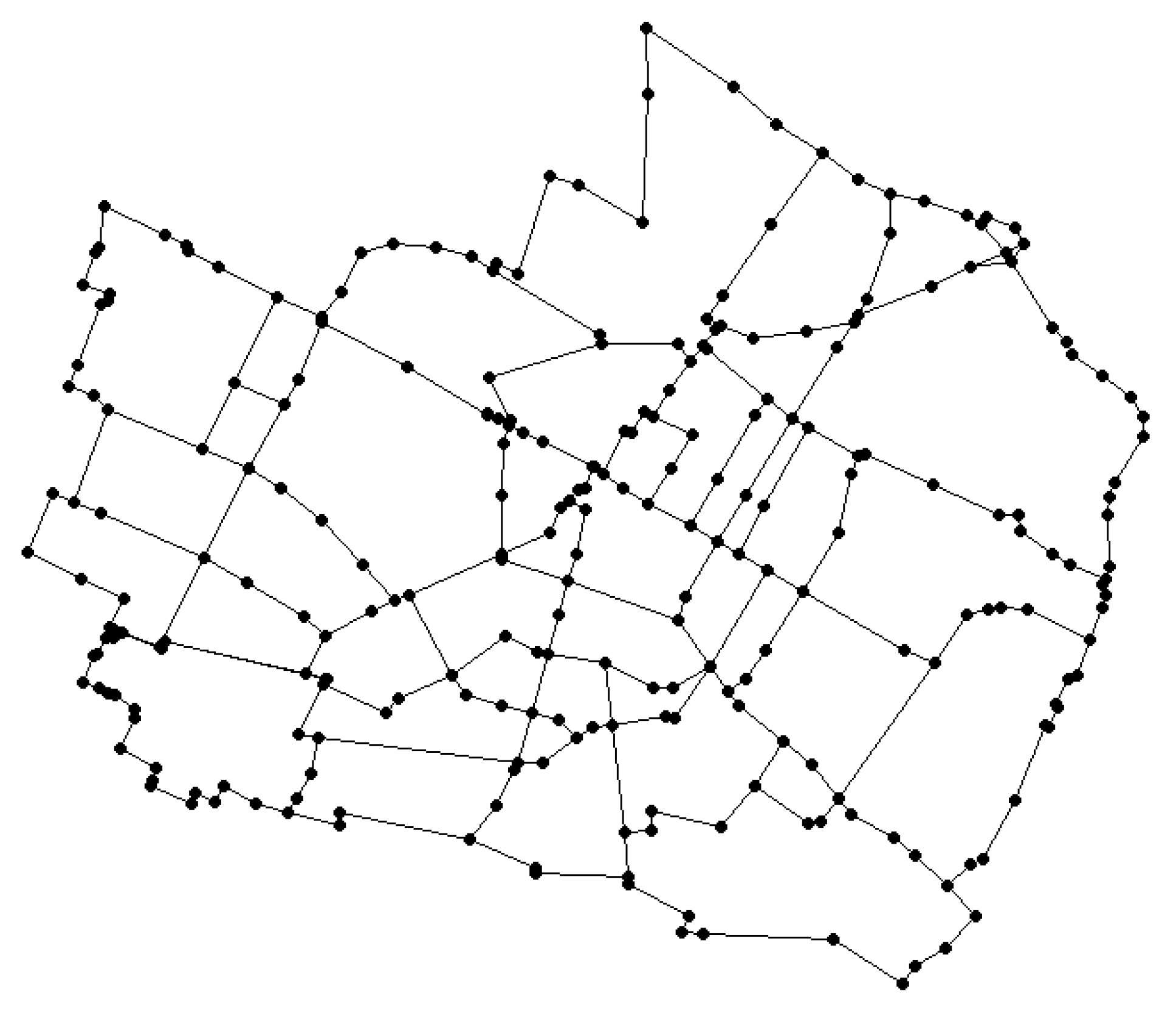
In this section, we analyze the SOH performance to show that it can compete with state-of-the-art nonlinear solvers when it runs multiple times using a multi-start procedure. The layout of the Modena network (Figure 2), which is available in [42], is used to compare the performance of the SOH against the nonlinear solver. For solving the nonlinear Q-C model, the IPOPT solver was used [31]. IPOPT is an open-source nonlinear optimization solver, which uses the interior-point algorithm. The experiment is programmed in MATLAB using the YALMIP modeling language [43], the code is available in GitHub Repository (https://github.com/SWSLAB/SOH/ (Accessed on 12 August 2021). The SOH algorithm is used with $\beta ={10}^6$, $\epsilon =0.001$ for all runs. IPOPT is used with default tuning parameters except for the maximum iteration limit, which is increased to one million iterations. In the absence of other studies that compare the performance of optimization algorithms on the Q-C model, we only compared the SOH to IPOPT. Future research can build on the code and data in the GitHub Repository to test the performance of other optimization heuristics compared to the proposed SOH.

We used the same network layout of the Modena network as in [42], but some of the configurations were randomly generated to create synthetic problems for testing the optimization solvers. For example, we have defined 30 sources and 50 demands nodes in the network that were randomly chosen. The demands, bounds, and costs were also randomly generated along the management horizon. The salinity levels in the source nodes are chosen such that the salinity is high for sources with low production cost, this characteristic will create a more challenging problem because of the tradeoff between meeting the quality constraints and minimizing the production cost. It is noteworthy that because the layout and pipe directions are predetermined in the Modena network, the feasibility of randomly generated problems is not guaranteed. For example, if a node that has only outgoing pipes is selected as a demand node, the problem will be infeasible, or if the total capacity of the links ingoing a demand node is below the required demand, the problem will be infeasible. In this study, we only consider randomly generated problems, which have feasible solutions. The configurations of the solved problems are available in https://github.com/SWSLAB/SOH/ (accessed on 12 August 2021).

To study the impact of model size on computation time and accuracy, a series of runs are made in which the number of years is increased from one to eight. For a single year, the nonlinear Q-C model (Equations (14)–(22)) of the Modena network includes 1191 decision variables. The size of the optimization problem will linearly increase with the management horizon. For $T=8$, the nonlinear optimization model will have 1191 × 8 = 9528 decision variables. Since both the SOH and IPOPT are local optimization solvers, we adapted a multi-start procedure in which the optimization problem is solved from 25 starting points, which are randomly drawn from uniform probability distribution defined by the decision variables bounds. At the end of the process, each solver will end up with a “bank” of 25 solutions for the problem. The selected solution from each solver is the one that is feasible and minimizes the objective function.

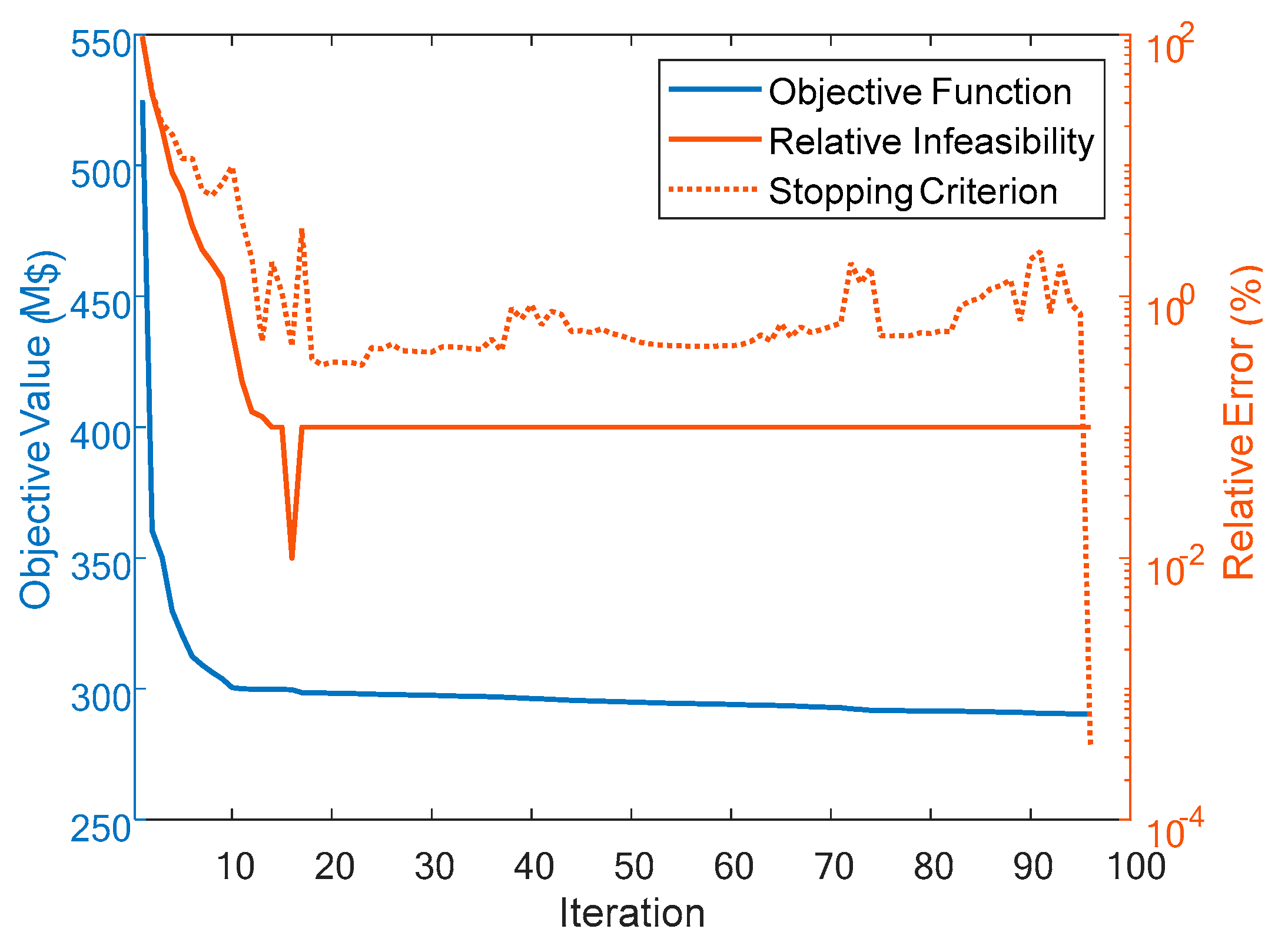
Before we start the comparison, Figure 3 demonstrates the iteration process in the SOH. Figure 3 shows the solution progress for the optimal run with $T=1$. In this run, the relative infeasibility is more than 1% up to iteration 10, and the objective function drops drastically in these first 10 iterations from 525 M$ to 300 M$. The relative infeasibility is within the tolerance $\epsilon =0.1\%$ starting from iteration 15, while the stopping criterion in Equation (37) is satisfied at iteration 96. The objective function improves from 299.7 to 290.4 M$ between iterations 15 and 96.

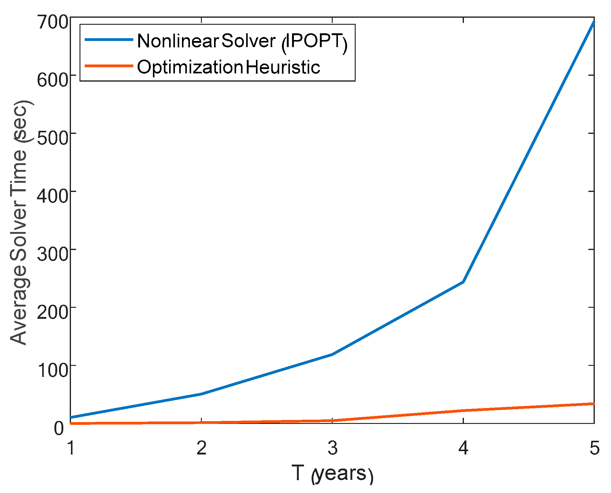
To compare the efficiency of the SOH and IPOPT, Figure 4 shows the average solver time for different problems with increasing size (number of decision variables ranges from 1191 to 5955), which are obtained by increasing the problem horizon from one year to five years. The results show that the solution time of the nonlinear solver is increasing exponentially with the problem size while the SOH solves the problems with a moderate increase in the solution time. For example, for a Q-C model with a horizon of five years, the solution time of the multi-start procedure using IPOPT is 25 × 693 = 17,325 s (~4.81 h) while using the SOH is 25 × 34 = 850 s (~0.24 h).

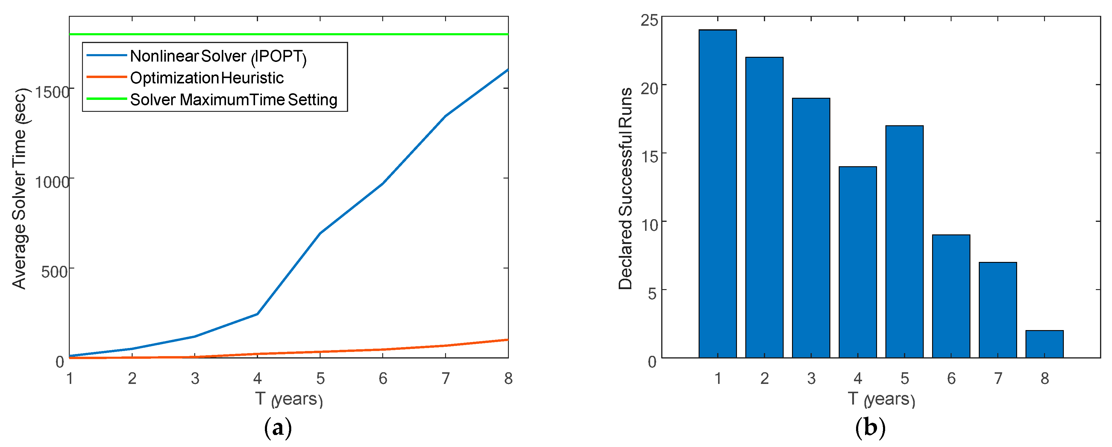
Further increasing the problem horizon will create larger problems in which the nonlinear solver will require a longer solution time. It is typical when using nonlinear solvers to limit the number of iterations or to limit the solver time. In Figure 5, the problem is further increased to 9528 decision variables by increasing the problem horizon to eight years. Nonetheless, to examine the practicality of the nonlinear solver, the IPOPT solver time limit is set to 1800 s (0.5 h). While the exponential increase in IPOPT solver is not maintained after $T=5$ (due to limiting the solver time), the difference between the solution time of the SOH and IPOPT is still evident, since the SOH shows an almost linear increase in solution time with respect to the problem horizon. For a large problem with 9528 decision variables, the multi-start procedure will require about 11 h using IPOPT, but only 0.7 h using the SOH. Moreover, for the largest problem, only two out of the 25 runs in IPOPT were declared successful (reached first-order optimality conditions), the rest of the runs either failed to converge to local optima or reached the maximum time limit. Figure 5 also shows the successful runs of IPOPT out of 25 for increasing problem horizon (i.e., increasing problem size).

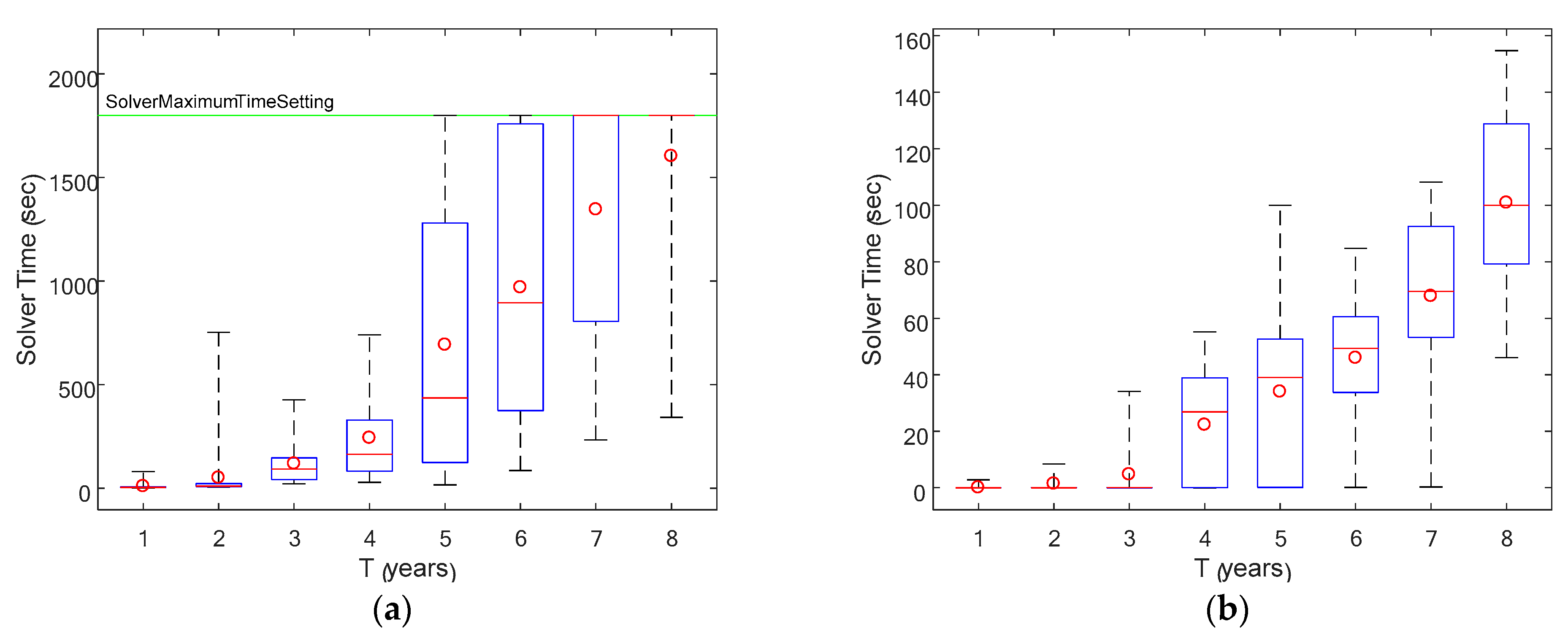
Figure 6 shows the box-and-whiskers plots for IPOPT and SOH solution time, respectively. The boxes show the interquartile ranges with the red crossbar depicting the median and the red circle depicting the mean. The whiskers show the minimum and maximum values. The results show that while IPOPT solver can reach the solution fast when the problem is small in most of the runs, the solution time becomes impractical for large problems as most of the runs reach the practical limit of 0.5 h per run. For example, when $T=8$, 20 out of 25 of the runs (i.e., 80%) reach the maximum time limit of the solver. On the other hand, the worst solution time of the SOH is 155 s.

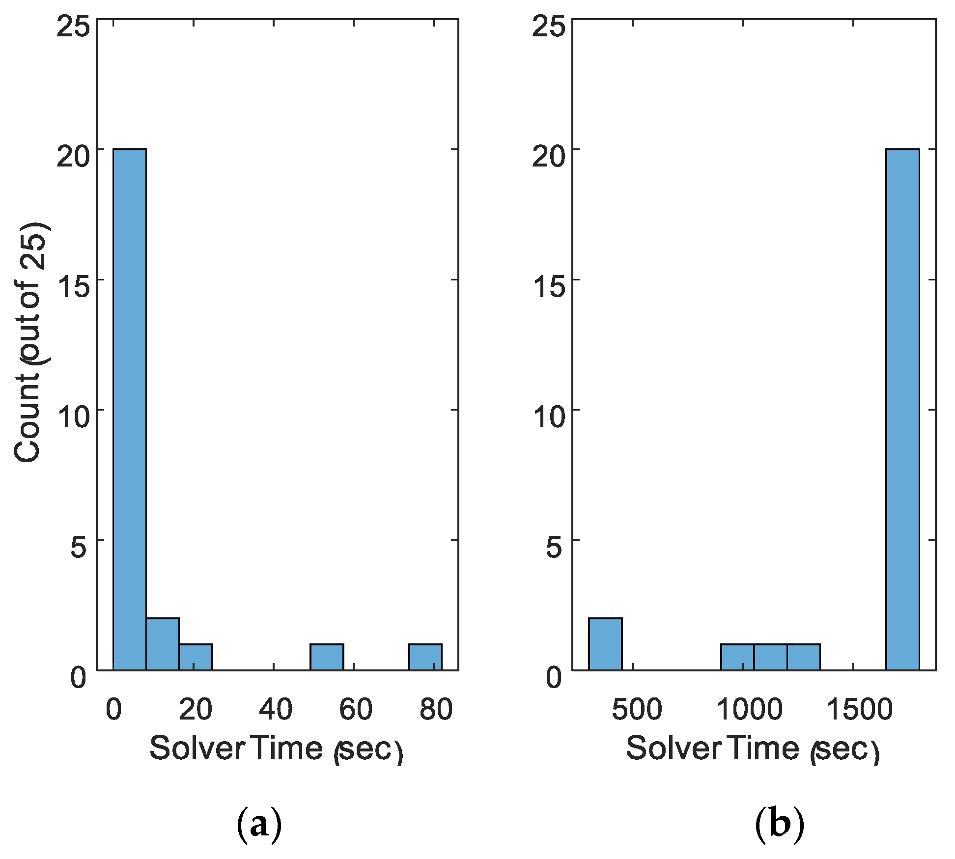
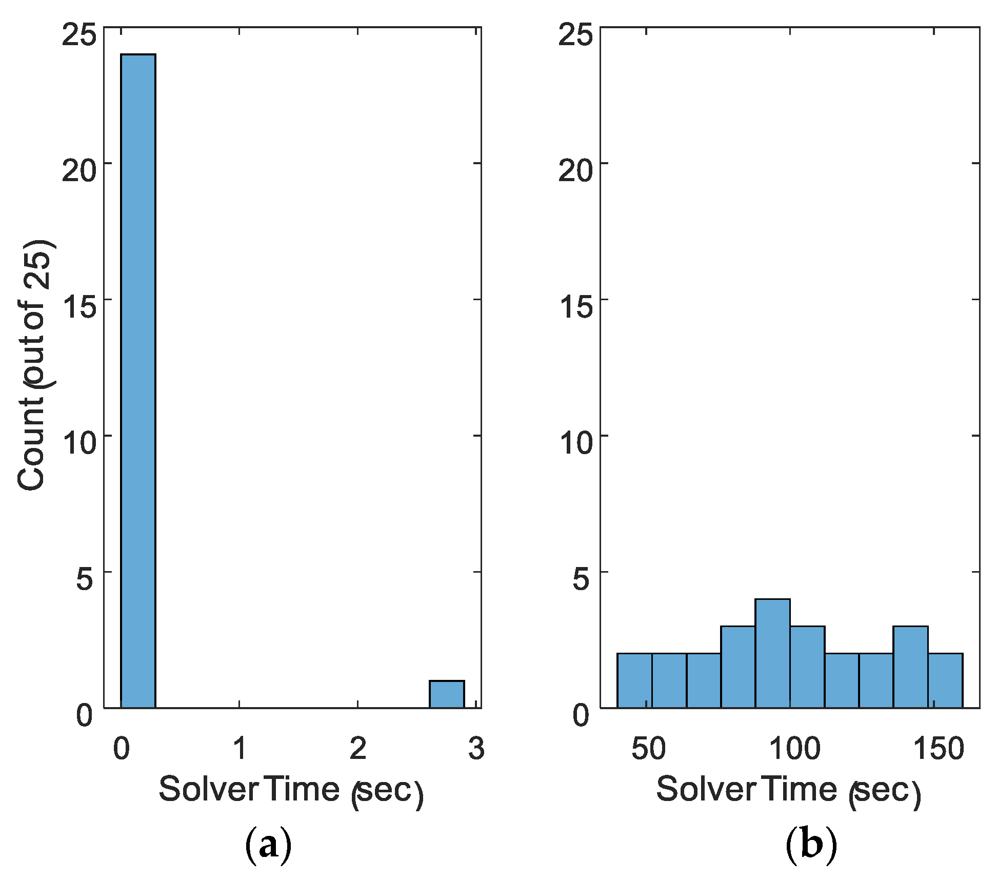
Figure 7 and Figure 8 show the detailed solver time histograms of the smallest and largest problem for IPOPT and SOH, respectively. In the smallest problem with $T=1$, 20 out of 25 the runs in IPOPT required a short run time of 6.6 s, however for the large problem with $T=8$, 20 out of the 25 runs reach the time limit. Figure 8 shows the solver time in the SOH for the small problem is less than 3 s in all runs, while for the large problem the solver time is almost uniformly distributed between 46–154.7 s.

In light of the above, it is clear that the SOH solves large problems much faster than the nonlinear solver, but the question to tackle next is: is it as accurate?

To answer this question we define the error between the best objective values obtained by the multi-start procedure using IPOPT and SOH as given in Equation (38).

$$ObjErr=\frac{OptOb{j}_{SOH}-OptOb{j}_{IPOPT}}{OptOb{j}_{IPOPT}}\times 100\%$$

(38)

Figure 9 shows the objective error, as defined in Equation (38), for increasing problem horizon (i.e., increasing problem size). The SOH shows good accuracy for all the solved problems. The worst-case error is as low as 0.45%. In fact, for $T>5$ the error is negative, indicating that the optimal objective value reached by the SOH is better than the optimal value obtained in IPOPT. For example, when $T=7$ the SOH optimal value is 0.32% better than the IPOPT solution. However, in general, the error is relatively low (regardless of its sign) and the two solutions could be considered identical for practical purposes.

To judge the quality of the solution it is not enough to examine the objective function, one should also examine the constraints violation of the problem. Figure 10 shows the relative infeasibility in the solute balance as defined in Equation (39).

$$RelInf=\frac{\Vert \hspace{0.17em}\hspace{0.17em}{\left[A\cdot \left(Q^{t*}\circ C^{t*}\right)\right]}_{\forall t}\Vert }{\Vert \hspace{0.17em}\hspace{0.17em}{\left[Q^{t*}\circ C^{t*}\right]}_{\forall t}\Vert }$$

(39)

where $Q^{t*},C^{t*}$ are the optimal decision values as obtained from the multi-start procedure using the SOH. The results in Figure 10 show that the relative infeasibility is below the acceptable tolerance of the SOH ( $\epsilon =0.1\%$) for all the solved problems.

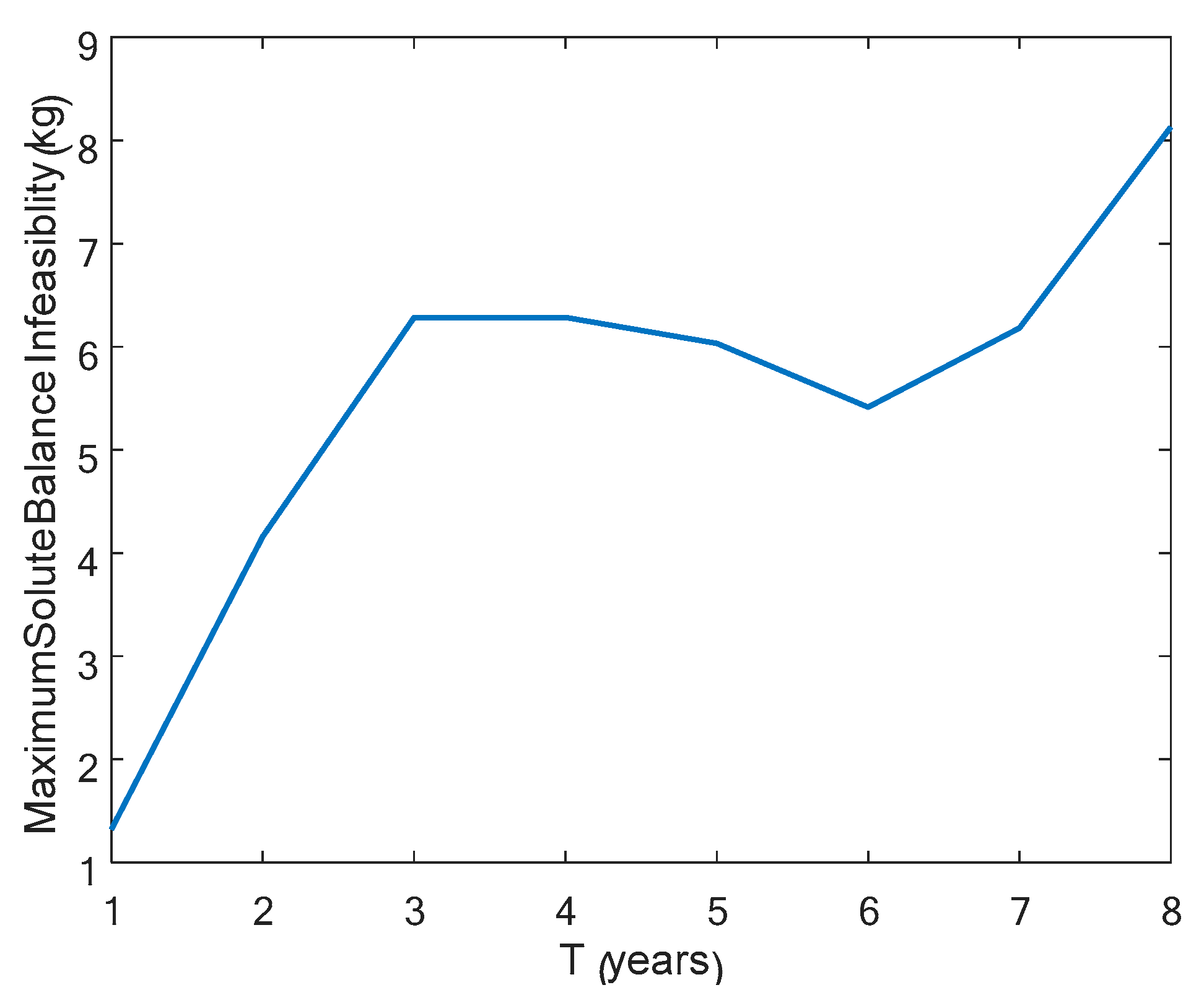
Figure 11 shows the maximum solute balance infeasibility as defined in Equation (40). The results in Figure 11 show that while maximum infeasibility is generally increasing with problem size, the maximum infeasibility is as low as 8.13 kg per year, which is a very negligible imbalance for practical regional water supply systems that deliver millions of cubic meters per year.

$$MaxInf=\max \left({\left[A\cdot \left(Q^{t*}\circ C^{t*}\right)\right]}_{\forall t}\right)$$

(40)

Solution efficiency is a key element for the practical implementation of Q-C models. Often, Q-C optimization models results will be used within Decision Support Systems to facilitate active discussion between stakeholders. A slow solution process will hinder real-time stakeholders’ interaction with the model in which scenarios (i.e., changing constraints or different parameters) are refined rapidly. In practice, it is hard to define the scenarios in advance; usually, the scenarios are refined during an active discussion between the stakeholders (partly by seeing how the model reacts). Near-real-time interaction with the model is very important, and it could be done only if the model can be solved in a reasonable time. Thus, a fast solution process can contribute to expediting stakeholders’ engagement with Decision Support Systems. Our results indicate that using simple optimization heuristics combined with a multi-start optimization procedure can be an alternative to off-the-shelf nonlinear solvers when solving multisource quantity-quality models. The results from the suggested approach compete with nonlinear solvers in terms of both accuracy and efficiency. The results show that for large-scale problems (five-year horizon) the nonlinear solver will require ~4.8 h, making it an impractical tool for near-real-time interactions with the model, while the suggested heuristic can solve the same problem in ~15 minutes. If we further increase the horizon to eight years (i.e., 9528 decision variables), the nonlinear solver will reach the maximum time limit of 1800 s in 80% of the runs, and the runtime will be as high as ~11 h which is compared to ~0.7 h when using the SOH. This efficiency of the SOH is obtained by harnessing ultra-fast optimization procedures within an iterative process. Moreover, the results show that SOH can reach good accuracy with maximum relative error in the objective function of 0.45% and relative infeasibility within the prescribed tolerance. Still, the SOH is a local solver (as well as the nonlinear solver, IPOPT), and thus, it cannot guarantee a globally optimal solution. In this study, we compared the performance of the nonlinear solver and the SOH using the same settings of the multi-start procedure (i.e., the same number of initial points). However, owing to the fast solution process of the SOH, we can consider a larger number of initial points, which will increase the chance to reach a globally optimal solution. Further research is needed to examine the performance of the proposed approach in reaching the global optimum compared to state-of-the-art global optimization solvers.

References

- Droogers, P.; Immerzeel, W.W.; Terink, W.; Hoogeveen, J.; Bierkens, M.F.P.; Van Beek, L.P.H.; Debele, B. Water resources trends in Middle East and North Africa towards 2050. Hydrol. Earth Syst. Sci. 2012, 16, 3101–3114. [Google Scholar] [CrossRef] [Green Version]
- Loucks, D.P.; van Beek, E. Water Resource Systems Planning and Management: An Introduction to Methods, Models, and Applications; UNESCO: Paris, France, 2005. [Google Scholar]
- Eusuff, M.M.; Lansey, K.E. Optimization of water distribution network design using the shuffled frog leaping algorithm. J. Water Resour. Plan. Manag. 2003, 129, 210–225. [Google Scholar] [CrossRef]
- Zaide, M. A Model for Multi-Year Combined Optimal Management of Quantity and Quality in the Israeli National Water Supply System. Doctoral Dissertation, Technion-Israel Institute of Technology, Haifa, Israel, 2006. Available online: https://shamir.net.technion.ac.il/files/2019/01/2011-Housh-Ostfeld-Shamir-RC-EWRI-2011.pdf (accessed on 11 May 2021).
- Tu, M.-Y.; Tsai, F.T.-C.; Yeh, W.W.-G. Optimization of water distribution and water quality by hybrid genetic algorithm. J. Water Resour. Plan. Manag. 2005, 131, 431–440. [Google Scholar] [CrossRef]
- Cohen, D.; Shamir, U.; Sinai, G. Optimal operation of multi-quality water supply systems-I: Introduction and the Q-C model. Eng. Optim. 2000, 32, 549–584. [Google Scholar] [CrossRef]
- Cohen, D.; Shamir, U.; Sinai, G. Optimal operation of multi-quality water supply systems-II: The Q-H model. Eng. Optim. 2000, 32, 687–719. [Google Scholar] [CrossRef]
- Cohen, D.; Shamir, U.; Sinai, G. Optimal operation of multiquality water supply systems-III: The Q-C-H model. Eng. Optim. 2000, 33, 1–35. [Google Scholar] [CrossRef]
- Wada, Y.; Van Beek, L.P.H.; Van Kempen, C.M.; Reckman, J.W.T.M.; Vasak, S.; Bierkens, M.F.P. Global depletion of groundwater resources. Geophys. Res. Lett. 2010, 37, 1–5. [Google Scholar] [CrossRef] [Green Version]
- Oude Essink, G.H.P. Improving fresh groundwater supply—Problems and solutions. Ocean. Coast. Manag. 2001, 44, 429–449. [Google Scholar] [CrossRef]
- Ma, T.; Sun, S.; Fu, G.; Hall, J.W.; Ni, Y.; He, L.; Yi, J.; Zhao, N.; Du, Y.; Pei, T.; et al. Pollution exacerbates China’s water scarcity and its regional inequality. Nat. Commun. 2020, 11, 1–9. [Google Scholar] [CrossRef] [PubMed] [Green Version]
- Vengosh, A.; Rosenthal, E. Saline groundwater in Israel: Its bearing on the water crisis in the country. J. Hydrol. 1994, 156, 389–430. [Google Scholar] [CrossRef]
- Jones, E.; Qadir, M.; van Vliet, M.T.H.; Smakhtin, V.; Kang, S. mu The state of desalination and brine production: A global outlook. Sci. Total Environ. 2019, 657, 1343–1356. [Google Scholar] [CrossRef] [PubMed]
- World Bank Group. The Role of Desalination in an Increasingly Water-Scarce World; World Bank: Washington, DC, USA, 2019. [Google Scholar]
- Dreizin, Y.; Tenne, A.; Hoffman, D. Integrating large scale seawater desalination plants within Israel’s water supply system. Desalination 2008, 220, 132–149. [Google Scholar] [CrossRef]
- Housh, M.; Ostfeld, A.; Shamir, U. Seasonal multi-year optimal management of quantities and salinities in regional water supply systems. Environ. Model. Softw. 2012, 37, 55–67. [Google Scholar] [CrossRef]
- Shah, M.; Sinai, G. Steady state model for dilution in water networks. J. Hydraul. Eng. 1988, 114, 192–206. [Google Scholar] [CrossRef]
- Mehrez, A.; Percia, C.; Oron, G. Optimal operation of a multisource and multiquality regional water system. Water Resour. Res. 1992, 28, 1199–1206. [Google Scholar] [CrossRef]
- Tawarmalani, M.; Sahinidis, N.V. Convexification and Global Optimization in Continuous and Mixed-Integer Nonlinear Programming: Theory, Algorithms, Software, and Applications; Springer: Berlin, Germany, 2002. [Google Scholar]
- Cai, X.; McKinney, D.C.; Lasdon, L.S. Integrated hydrologic-agronomic-economic model for river basin management. J. Water Resour. Plan. Manag. 2003, 129, 4–17. [Google Scholar] [CrossRef] [Green Version]
- Yates, D.; Purkey, D.; Sieber, J.; Huber-Lee, A.; Galbraith, H. WEAP21—A demand-, priority-, and preference-driven water planning model. Part 2: Aiding freshwater ecosystem service evaluation. Water Int. 2005, 30, 501–512. [Google Scholar] [CrossRef]
- Jenkins, M.W.; Lund, J.R.; Howitt, R.E.; Draper, A.J.; Msangi, S.M.; Tanaka, S.K.; Ritzema, R.S.; Marques, G.F. Optimization of California’s water supply system: Results and insights. J. Water Resour. Plan. Manag. 2004, 130, 271–280. [Google Scholar] [CrossRef] [Green Version]
- Draper, A.J.; Jenkins, M.W.; Kirby, K.W.; Lund, J.R.; Howitt, R.E. Economic-engineering optimization for california water management. J. Water Resour. Plan. Manag. 2003, 129, 155–164. [Google Scholar] [CrossRef]
- Ostfeld, A.; Shamir, U. Optimal operation of multiquality networks. I: Steady-state conditions. J. Water Resour. Plan. Manag. 1993, 119, 645–662. [Google Scholar] [CrossRef]
- Ostfeld, A.; Shamir, U. Design of optimal reliable multiquality water-supply systems. J. Water Resour. Plan. Manag. 1996, 122, 322–333. [Google Scholar] [CrossRef]
- Schwarz, J.; Meidad, N.; Shamir, U. Water quality management in regional systems. IAHS-AISH Publ. 1985, 153, 341–349. [Google Scholar]
- Fukuda, E.H.; Graña Drummond, L.M. On the convergence of the projected gradient method for vector optimization. Optimization 2011, 60, 1009–1021. [Google Scholar] [CrossRef]
- Gill, P.; Murray, W.; Murtagh, B.; Saunders, M.; Wright, M. GAMS/MINOS in GAMS: Solver Manuals; GAMS Development Corp.: Washington, DC, USA, 2000. [Google Scholar]
- Shor, N.Z. Minimization Methods for Non-Differentiable Functions; Springer: Berlin, Germany, 1985; Volume 3, ISBN 978-3-642-82120-2. [Google Scholar]
- Gabriele, G.A.; Ragsdell, K.M. Large scale nonlinear programming using the generalized reduced gradient method. J. Mech. Des. Trans. ASME 1980, 102, 566–573. [Google Scholar] [CrossRef]
- Biegler, L.T.; Zavala, V.M. Large-scale nonlinear programming using IPOPT: An integrating framework for enterprise-wide dynamic optimization. Comput. Chem. Eng. 2009, 33, 575–582. [Google Scholar] [CrossRef]
- Cai, X.; McKinney, D.C.; Lasdon, L.S. Solving nonlinear water management models using a combined genetic algorithm and linear programming approach. Adv. Water Resour. 2001, 24, 667–676. [Google Scholar] [CrossRef]
- Griffith, R.E.; Stewart, R.A. A Nonlinear Programming Technique for the Optimization of Continuous Processing Systems. Manage. Sci. 1961, 7, 379–392. [Google Scholar] [CrossRef]
- Palacios-Gomez, F.; Lasdon, L.; Engquist, M. Nonlinear optimization by successive linear programming. Manag. SCI 1982, 28, 1106–1120. [Google Scholar] [CrossRef]
- Nocedal, J.; Wright, S. Numerical Optimization; ser. Springer Series in Operations Research; Springer: New York, NY, USA, 1999. [Google Scholar]
- Byrd, R.H.; Gilbert, J.C.; Nocedal, J. A trust region method based on interior point techniques for nonlinear programming. Math. Program. 2000, 89, 149–185. [Google Scholar] [CrossRef] [Green Version]
- Palomares, U.M.G.; Mangasarian, O.L. Superlinearly convergent quasi-newton algorithms for nonlinearly constrained optimization problems. Math. Program. 1976, 11, 1–13. [Google Scholar] [CrossRef] [Green Version]
- Powell, M.J.D. A fast algorithm for nonlinearly constrained optimization calculations. In Numerical Analysis; Springer: Berlin/Heidelberg, Germany, 1978; pp. 144–157. [Google Scholar]
- Di Pillo, G.; Grippo, L. Exact penalty functions in constrained optimization. SIAM J. Control Optim. 1989, 27, 1333–1360. [Google Scholar] [CrossRef]
- CPLEX IBM ILOG CPLEX Optimization Studio. 2017. Available online: https://www.ibm.com/docs/SSSA5P_12.8.0/ilog.odms.studio.help/pdf/usrcplex.pdf (accessed on 11 May 2021).
- Brent, R.P. Algorithms for minimization without derivatives. IEEE Trans. Automat. Contr. 1974, 19, 632–633. [Google Scholar] [CrossRef] [Green Version]
- Exeter Benchmarks. Available online: http://emps.exeter.ac.uk/engineering/research/cws/resources/benchmarks/design-resiliance-pareto-fronts/data-files/ (accessed on 24 July 2021).
- Löfberg, J. YALMIP: A toolbox for modeling and optimization in MATLAB. In Proceedings of the IEEE International Symposium on Computer-Aided Control System Design, Taipei, Taiwan, 2–4 September 2004; pp. 284–289. [Google Scholar]
Figure 1.
Illustrative network.
Figure 2.
Layout of Modena network.
Figure 3.
Iteration process for the optimal run of .
Figure 4.
Average solution time for without solver time limit.
Figure 5.
(a) Average solution time for with solver time limit of 1800 seconds; (b) Successful runs of IPOPT out of 25 for .
Figure 6.
Box-and-whiskers plots for IPOPT (a) and SOH (b) solution time.
Figure 7.
Histogram of IPOPT solver time for the small (a) and the large (b) problems.
Figure 8.
Histogram of SOH solution time for the small (a) and the large (b) problems.
Figure 9.
Objective error for the SOH compared to the best solution from IPOPT.
Figure 10.
Relative infeasibility using the SOH.
Figure 11.
Maximum infeasibility using the SOH.5. Conclusions.