
Factors Governing Biodegradability of Dissolved Natural Organic Matter in Lake Water


1
Center of Biogeochemistry in the Anthropocene, Department of Chemistry, University of Oslo, P.O. Box 1033, 0371 Oslo, Norway
2
Center of Biogeochemistry in the Anthropocene, Department of Biosciences, University of Oslo, P.O. Box 1066, 0371 Oslo, Norway
*
Author to whom correspondence should be addressed.
Water 2021, 13(16), 2210; https://doi.org/10.3390/w13162210
Submission received: 31 May 2021
/
Revised: 18 July 2021
/
Accepted: 9 August 2021
/
Published: 13 August 2021
(This article belongs to the Special Issue Freshwater Ecosystems under Anthropogenic Stress)
Abstract
:Dissolved Natural Organic Matter (DNOM) is a heterogeneous mixture of partly degraded, oxidised and resynthesised organic compounds of terrestrial or aquatic origin. In the boreal biome, it plays a central role in element cycling and practically all biogeochemical processes governing the physico-chemistry of surface waters. Because it plays a central role in multiple aquatic processes, especially microbial respiration, an improved understanding of the biodegradability of the DNOM in surface water is needed. Here the current study, we used a relatively cheap and non-laborious analytical method to determine the biodegradability of DNOM, based on the rate and the time lapse at which it is decomposed. This was achieved by monitoring the rate of oxygen consumption during incubation with addition of nutrients. A synoptic method study, using a set of lake water samples from southeast Norway, showed that the maximum respiration rate (RR) and the normalised RR (respiration rate per unit of carbon) of the DNOM in the lakes varied significantly. This RR is conceived as a proxy for the biodegradability of the DNOM. The sUVa of the DNOM and the C:N ratio were the main predictors of the RR. This implies that the biodegradability of DNOM in these predominantly oligotrophic and dystrophic lake waters was mainly governed by their molecular size and aromaticity, in addition to its C:N ratio in the same manner as found for soil organic matter. The normalised RR (independently of the overall concentration of DOC) was predicted by the molecular weight and by the origin of the organic matter. The duration of the first phase of rapid biodegradation of the DNOM (BdgT) was found to be higher in lakes with a mixture of autochthonous and allochthonous DNOM, in addition to the amount of biodegradable DNOM.
1. Introduction
The amount of Dissolved Natural Organic Matter (DNOM) in boreal surface waters typically exceeds in mass the content of inorganic constituents, and carbon associated with DNOM by far exceeds the biotic pools of C [1]. This DNOM, being a very heterogeneous mix of partly degraded organic compounds, has a profound effect on the cycling of carbon (C) and associated elements such as nitrogen (N) and phosphorus (P), in addition to the physicochemical characteristics of surface waters. During recent decades, the concentrations of DNOM in surface water have increased, especially in boreal lakes [2]. In these aqueous systems most of the DNOM is allochthonous, i.e., derived from the catchment [3]. The main driver for the ongoing rise in DNOM is the increase in terrestrial biomass (greening), rendering more organic matter in the soils available to be partly decomposed and leached out, causing surface water browning [4,5]. This is due to the rise in mean temperatures and to the increase in forest biomass [6], which, e.g., reached 29% in southeast Norway between 1971 and 2000 [7]. A concomitant factor is the increasing runoff and runoff intensity. This causes shifts in soil–water flow paths, with more water flowing through the organic-rich forest floor horizons before entering the stream, bypassing the absorptive capacity of the deeper mineral soil. A third major factor applies to regions heavily exposed to acid deposition in the 1970–1980s. Since then, sulphur (S) deposition has decreased by up to 90% in the previously most affected areas in southern Norway. The subsequent decrease in ionic strength, in addition to Al3+ and H+ concentrations, has increased DNOM solubility and reduced its flocculation, increasing its flux to surface waters [8,9]. However, the decrease in S deposition has subsided, and the effect of this driver no longer contributes significantly to the present increase in DNOM.
The increased concentrations of DNOM in lakes have, in turn, significant impacts on the lake ecosystem. The increasing content of chromophoric DNOM (CDOM) reduces light penetration and thereby the depth of photosynthetic active radiation [10]. Concurrently, the increased contribution of allochthonous carbon boosts microbial metabolism and therefore enhances heterotrophic respiration. This is potentially boosting the net emission of the greenhouse gases (GHGs) CO2 and CH4 [11], promoting the role of boreal lakes as hot-spots for GHG emissions [3].
The bioavailability of DNOM to bacterial respiration is known to mainly depend on its molecular weight and aromaticity, with the low molecular weight (LMW) and more saturated moieties of the DNOM being most biodegradable [12]. Allochthonous DNOM has a generally higher molecular weight (HMW) and is more aromatic than DNOM produced in situ (autochthonous) [13]. Nevertheless, due to the large flux of DNOM from boreal catchments, the allochthonous DNOM constitutes a significant fraction of the bioavailable organic C in their surface waters. In addition, the DNOM contents of key nutrients, such as N and P, are important for both autotroph and heterotroph production of boreal lakes [11]. In addition, photodegradation, or photobleaching, transforms the aromatic HMW DNOM moieties into more saturated and more LMW DNOM compounds that are thus more bioavailable [14]. Insights into the factors governing the microbial respiration of DNOM (i.e., its biodegradability) are important for assessing the transformation of organic C to CO2.
The objective of this study was to assess the temporal dynamics of DNOM biodegradability in a wide range of boreal lakes with different quantities and qualities of DNOM. This measure of biodegradability differs from end-point measurements of the biodegradable amount of organic carbon (BDOM), estimated either by the decline in oxygen concentration or the increase in CO2 emissions, or by analysing the content of DOC [15]. During incubation, the decline in oxygen (O2) concentration is monitored over time with gas sensors, providing a measure of the maximum speed at which bacteria consume O2 (i.e., respiration rate (RR), DOC normalised RR (RRn), and duration of rapid biodegradation (BdgT)) that relates to the physicochemical properties of the DNOM and other water quality properties. Optical sensors for dissolved oxygen have previously been used to measure the biodegradability of organic pollutants under incubation [16]. The estimation of the respiration rate of organic matter with optical sensors has been previously undertaken in our group [17,18,19,20]. The large scale of the current study allows a standardisation of the method, including the development of a script for the extraction of biodegradability parameters and the comparison of the respiration rates in a large variety of samples.
2. Materials and Methods
2.1. Water Sampling
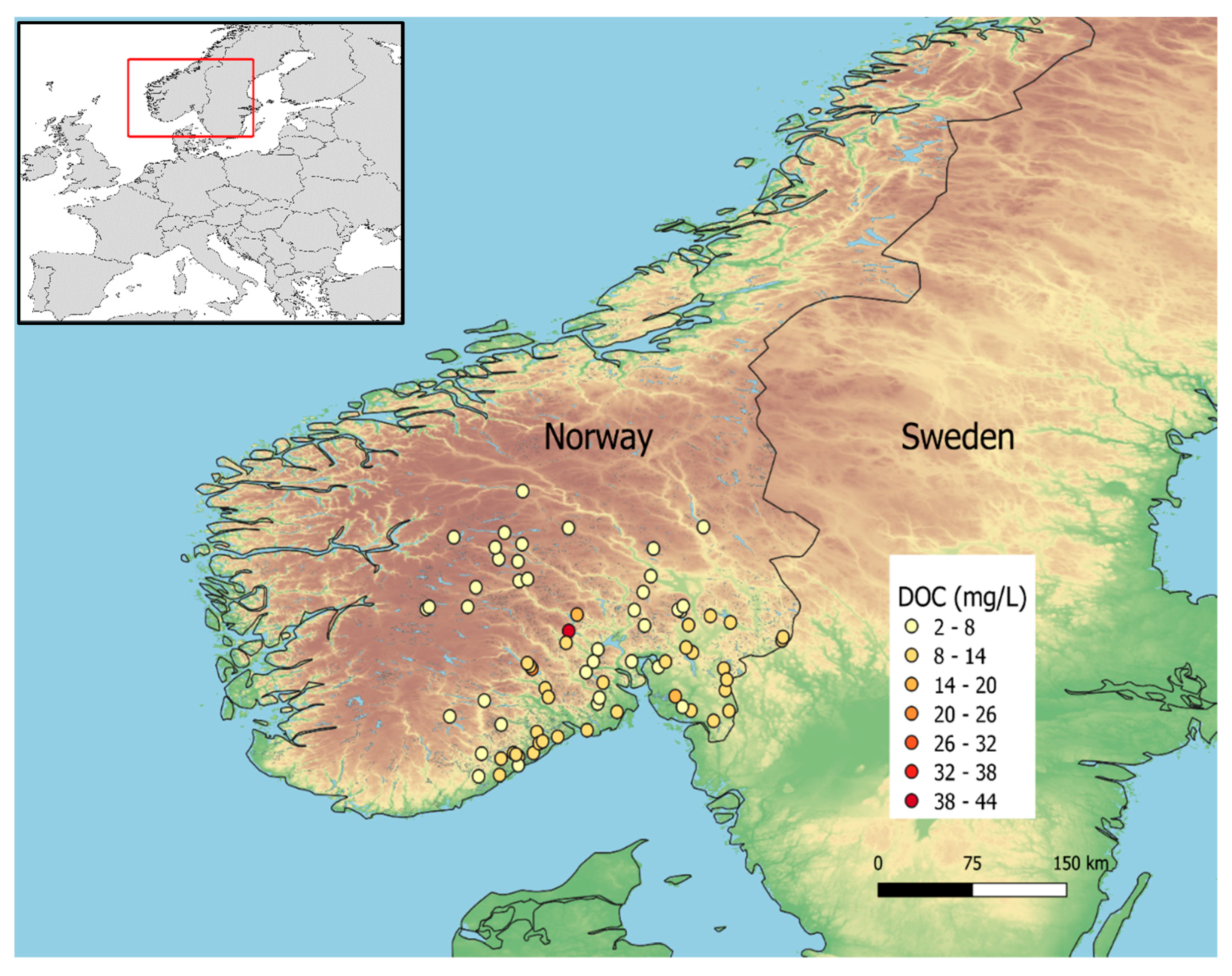
Surface water samples from 73 lakes in southeast Norway (Figure 1) were collected in autumn 2019 for detailed biogeochemical studies by the Centre for Biogeochemistry (CBA) at the University of Oslo, Norway. They were selected as a subset of the lakes sampled during the national lake survey, itself repeating the sampling of previous campaigns conducted in 1986 and 1995 [21,22]. These lakes span a wide range of water quality properties, notably DNOM, covering different catchment sizes and elevations. Most Norwegian lakes are oligotrophic or dystrophic, although a few of the lakes in the selection have mesotrophic or eutrophic characteristics (Figure S1).
2.2. Explanatory Water Quality Factors
The biodegradability of DNOM (RR, RRn and BdgT) from the 73 sampled lakes was related to more than 80 variables, describing the DNOM quality, in addition to the physical, chemical, and biological characteristics of the lake samples. The complete dataset and details about the experimental settings for the measurement of these variables are available on an online repository dedicated to the survey [23] and a summary is available in the Supplementary Material (Table S1). From these 80 parameters, 27 were selected as explanatory parameters based on their conceptual relevance. Empirical and conceptual links between the derived biodegradability descriptors and the following explanatory parameters were thus assessed: DOC normalised UV and VIS absorbance (sUVa = Aλ254 nm/DOC, sVISa = Aλ400 nm/DOC), UV/VIS absorbance ratio (SARuv), and spectral slope ratio (SR = Aλ275–295/Aλ350–400), along with DOC concentration, pH, alkalinity, lake temperature (T), conductivity (EC), O2, CO2, N2O and CH4 concentration, consumption and production, major cations (Calcium (Ca), Magnesium (Mg), Sodium (Na), Potassium (K)) and anions (Sulphate (SO4), Chloride (Cl)), Iron (Fe), Aluminium (Al), dissolved reactive Nitrogen and -Phosphorus (DN, DP), carbon to nutrient ratios (C:N, C:P), and bacterial abundance. The gas concentration, consumption, and production were obtained from a concomitant experiment, independent of the biodegradability measurements [11,24]. It should be noted that the nutrient concentrations applied for the statistical analysis is the original concentration in the sample water, not the concentration after the addition of nutrients for the incubation experiment.
As commonly found for environmental concentration variables, most of the ion and nutrient concentration data were not normally distributed, but rather skewed towards higher concentrations. Therefore, the concentration data were log transformed prior to analysis, except for pH, which is already in logarithmic form. Optical proxies of DNOM characteristics and cell counts where normally distributed and thus not log transformed. The dataset was standardised prior to regression analysis in order to ease the comparison of the effect size [25].
2.3. Determination of Biodegradability
A detailed description of the experiment protocol is available online [26] and provided in the Supplementary Material (Chapter B). The main principles and concepts are summarised in the following.
2.3.1. Sample Preparation for Biodegradability Analysis
At the sampling sites, a bucket of raw water was collected with a sampling rod close to the outlet of the lake, approximately 4 m from the shore. A quantity of 50 mL of raw water was filtered through a sterile 0.22 µm cartridge (Sterivex-GP Pressure unit filter, rinsed by pipetting 120 mL raw water through cartridge before sampling) to remove bacteria and eucaryotes. The samples were transported and stored at 10 °C in polyethylene bottles. Biodegradability measurements were conducted within 7 days after sampling. All batches of inoculum were prepared from a 50 L sample of water containing natural microbial communities (mainly bacteria) collected on September 8th, 2019, from one of the 73 sites, the dystrophic lake Langtjern ecological monitoring station (NIVA, 2021). After sampling, the water was filtered through 2.0 µm Isopore Membrane Filters to remove zooplankton. The water was then stored until use at in a closed tank at 10 °C with water circulation.
Three to five days prior to each incubation, the inoculum was prepared with 100 mL of the filtered water withdrawn from the tank and 1 mL of a solution of nutrients (5 mM ammonium nitrate and 5 mM dipotassium phosphate) to ensure unlimited growth of the bacterial community.
2.3.2. Incubation
The inoculum was added to each sample prior to the incubation, along with ample amounts of nutrients (same solution of 2:1 N:P as for the inoculum). N and P were added to ensure that the only limitation for the respiration rate at maximum O2 consumption was the biodegradability of the DNOM substrate, and thus that the biodegradability was primarily governed by the DNOM quantity and quality. A quantity of 0.25 mL of the inoculum solution and 0.25 mL of nutrient solution were added to 25.0 mL of the water sample, which means that 1% of the sample volume was added of both solutions. Therefore, the final concentration of nutrients in the biodegradation samples was 4- to 20-fold higher than that of the lake water with respect to N, and around 1000-fold for P. Aliquots of 5 mL samples were transferred into gas-tight PreSens SensorVials and placed on a PreSens plate (PreSens Precision Sensing, Regensburg, Germany) that holds 24 vials. Five samples with 4 replicates each were run in parallel, along with 3 blanks (5 mL of Type-1 water) and a house standard (solution of 20 mg C/L, prepared from Reverse Osmosis and freeze-dried isolate from Hellerudmyra, the source of The Nordic Humus Standard [27]). We did not include samples without added nutrients, because pilot studies showed very little biodegradation during the incubation period in that case. The 5 mM concentration for the stock solution of phosphate and ammonium nitrate was based on pilot studies, showing an increasing effect on biodegradation up to 5 mM, which levelled off above this concentration.
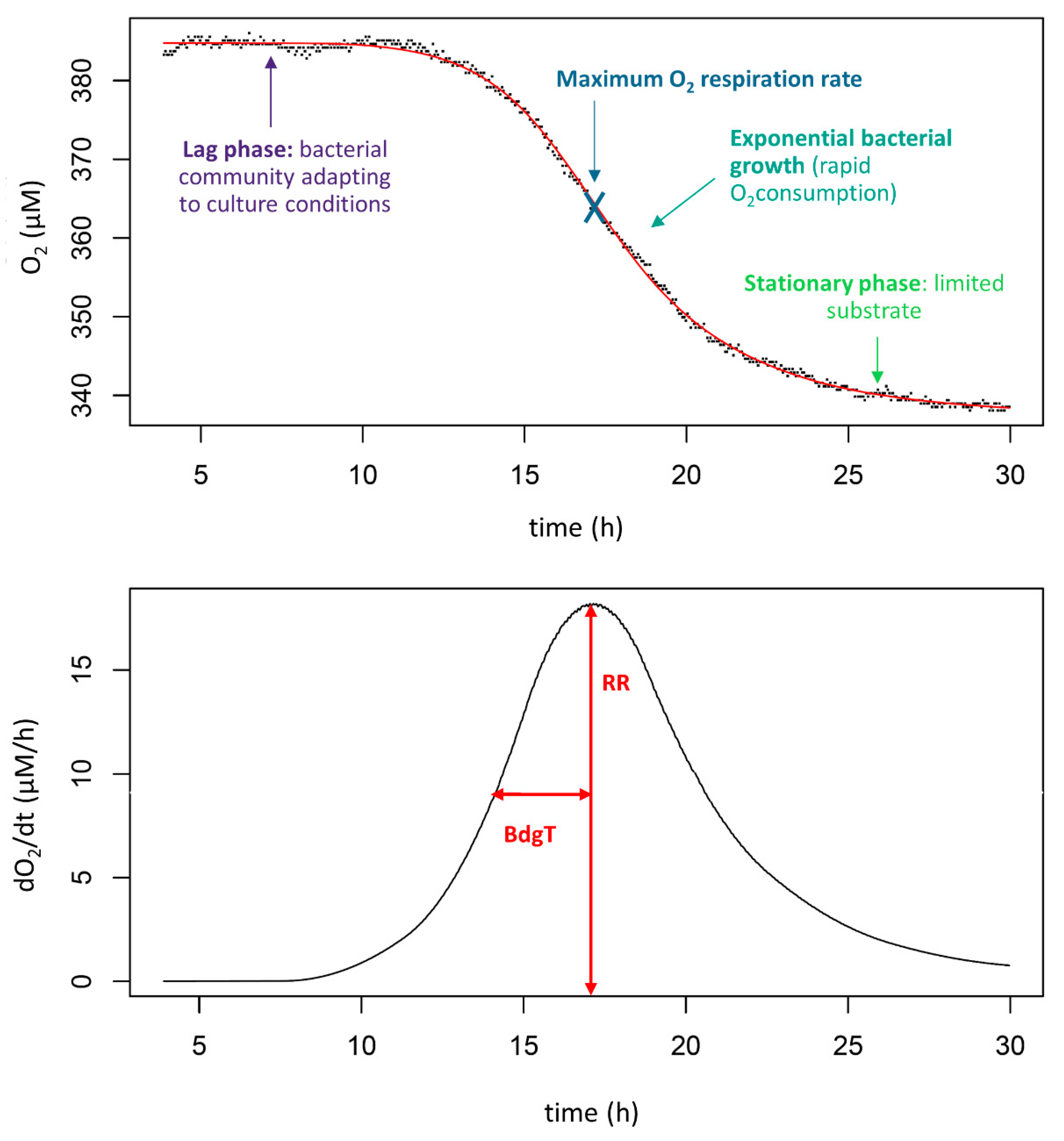
Three phases are commonly observed during incubation experiments [28]. During the initial phase, or “lag phase”, the inoculated bacterial community adapts to its new environment and substrate. During this phase oxygen consumption is low. Some activity is nevertheless taking place because the bacteria are synthesising new enzymes adapted to the new substrate, though no significant biodegradation occurs [28]. Following this phase, the bacterial respiration of the DNOM increases. The maximum rate of oxygen consumption obtained during a linear phase is used as a measure of RR of the DNOM and thus a proxy for its biodegradability. Eventually, a decrease in respiration occurs due to limitation in BDOM, lack of O2, or an accumulation of toxic wastes from the bacterial community. This phase subsides on a stationary plateau where the decrease in O2 is low.
2.3.3. Inoculum Composition
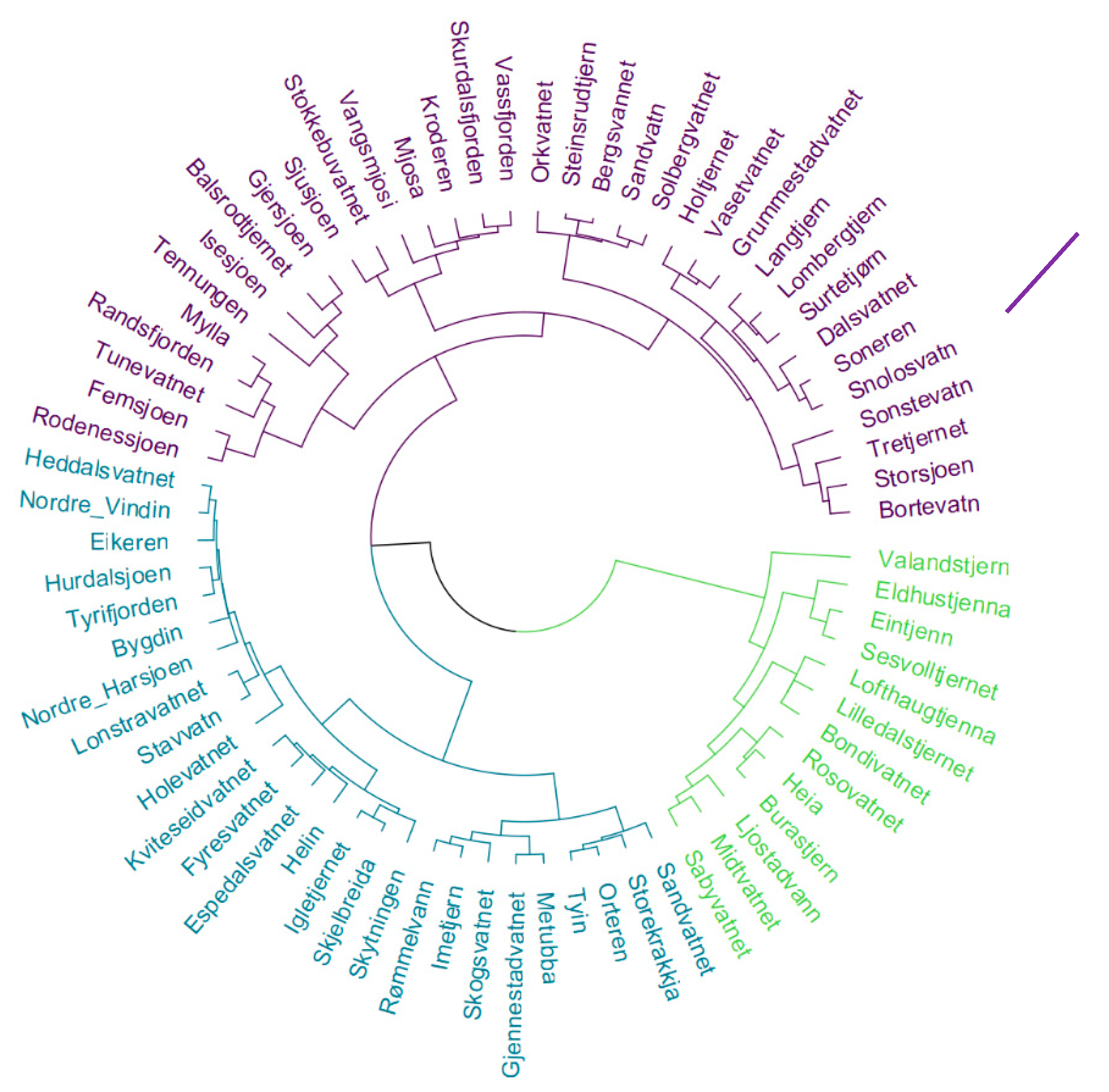
A standardised inoculum from one site was used in this study. This could represent a bias relative to site-specific properties and CDOM qualities. It was nevertheless assumed that the large biodiversity of bacteria in freshwater enables the population to adapt during the lag phase to the range of water qualities and DNOM substrates assessed in this study [29]. To test the assumption of microbial similarity, the bacterial community composition in Langtjern (the origin of the inoculum) was compared with that of the other 72 lakes. For this purpose, the Sterivex filter cartridges, used to remove bacteria and eucaryotes from the samples (Section 2.3.1), were liquid nitrogen frozen immediately after use on-site. Total DNA was extracted from each filter using a DNesay PowerWater Sterivex Kit (Qiagen, Hilden, Germany). Bacterial SSU rRNA gene amplicons were sequenced using an Illumina MiSeq with a 2 × 300 bp chemistry MiSeq (Illumina, San Diego, USA) at IMR sequencing facility (Dalhousie University, Halifax, Canada) following procedures from Comeau et al. [30]. As forward and reverse primers, 515FB (5’-GTGYCAGCMGCCGCGGTAA-3’) and 806RB (5’-GGACTACNVGGGTWTCTAAT-3’) were used, respectively. Raw sequences were trimmed of primers with CUTADAPT [31] and analysed with the R package dada2, version 1.18.0 [32] for de-replicating, de-noising, and sequence-pair assembly. Finally, taxonomy was assigned using the SILVA138 database.
A total of 1181 genera were found, confirming the large diversity of bacteria. To simplify the analysis, the genera, families, and orders were grouped by class taxonomic rank so that the sample sites could be clustered depending on the number of occurrence of bacteria from a given class. The ideal number of clusters was determined using the silhouette method [33]. This resulted in 3 site clusters, represented in Figure 2. An analysis of variance of the dependent variables based on these three clusters is presented in Section 3.1. All the computations were performed using the “factoextra” [34] and “dendextend” [35] packages in R.
2.3.4. Instrumentation
PreSens Oxygen sensors measure the oxygen concentration in samples by its quenching of fluorescence decay (PreSens Precision Sensing, Regensburg, Germany). The sensors contain a dye that is excited once every minute. The dye subsequently emits a fluorescence signal detected by the instrument. Oxygen molecules present in the solution collide with the excited dye, quenching the fluorescence, and thereby decreasing its intensity. Hence, the higher the oxygen concentration, the more collisions and the shorter the fluorescence lifetime. The lifetime of the fluorescence is recorded and converted to oxygen concentration using the Stern–Volmer equation. The oxygen sensors are situated in the bottom of the Sensor Vials, which are set on a plate with 24 wells. The plates are mounted on the Sensor Reader in an incubator (Digital incubator Incu-line 23 L, VWR International, Oslo, Norway), maintaining a constant temperature at 25 °C during the 30 h incubation period. The incubation time was chosen empirically as the time at which most samples have reached the last phase plateau.
2.3.5. Data Processing
The oxygen concentration in each vial was monitored every minute by the PreSens software (SDR_v4.0.0). Typically, the curve of oxygen concentration with time had a negatively sigmoid shape (Figure 3). A R script was developed to extract descriptive parameters for the biodegradability of DNOM from each curve by the following steps.
Data were removed from the initial hours of incubation, due to an unstable temperature and the lag phase (Section 2.3.2), and measurement after 30 h.
- The oxygen concentration values ([O2]t,initial) were normalised ([O2]t,corrected) by the ratio of oxygen concentration in the corresponding blanks ([O2]t,blank) divided by the mean of all the blanks, according to the following equation:
- The decline in oxygen concentration in each vial was fitted as a constrained spline (median R2 = 0.97) and the derivative of the equation was calculated (“scam” and “base” package on R). Typically, the derivative curve displays a peak, corresponding to the maximum rate of oxygen consumption. Two parameters were extracted from this peak, as shown in Figure 4: the maximum respiration rate (RR) and the biodegradation period (BdgT). The first half of the peak was used to determine the BdgT to avoid effects of limited O2 or accumulation of toxic wastes from the bacterial community (Section 2.3.2).
- RR and BdgT (Table 1) were determined for each of the 73 lakes as the median of 4 replicate samples. The area under the curve of the derivative was strongly correlated with RR (r = 0.93). It thus provided no new information and was therefore not included in the assessment.
2.4. Assessment of Factors Governing Biodegradability
Statistical analysis was conducted in R 4.0.3 [30], using the 27 conceptually relevant parameters selected from the CBA-100 lakes survey as predictors (Section 2.2) for the respiration rate (RR), normalised RR (RRn), and the biodegradability period (BdgrT) as response variables. The response variables and the relevant parameters, and the summary statistics of the 73 lakes, are presented in the Supplementary Material (Part A Table S1). Eight missing values in the dataset (summarised in the last column of the Table S1) were imputed by multiple imputation (50 imputations) using the “mice” package in R [36]. The multiple imputations process is described in the Supplementary Material, Part B Figure S5.
Correlation analysis on parameters that were not normally distributed was also conducted on log-transformed data (Section 2.2). A screening of the covariates was then performed to remove covariates with high correlations [37], using the correlation matrix (“micombine.cor”) function in the mice package.
Multivariate analysis was performed using a lasso (least absolute shrinkage and selection operator) regression model [38] on the 50 imputed datasets. The lasso model selects relevant parameters by shrinking the estimates of unimportant variables to 0. The estimates are selected by minimising the expression , where RSS is the residual sum of squares in the model, and λ is the penalty term used to shrink the estimate β [39]. Several λ might be obtained depending on how the dataset is separated between a training and a test subset. Cross-validation was applied to each model to select the best lambda (penalty) parameter each time, and the estimates of the covariates were computed and pooled. Pooling of lasso estimates consists of averaging the estimates for each dataset if the estimates were retained for more than half of the 50 lasso regression results. These analyses were undertaken using the cv.glmnet function in the “glmnetUtils” package in the R software environment [40]. The selected parameters were used to compute a multiple linear regression model (“Gauss-lasso regression”). The merits of the resulting models were compared by their mean absolute error (MAE).
3. Results
3.1. Respiration Rate and Time-Lapse of Biodegradability
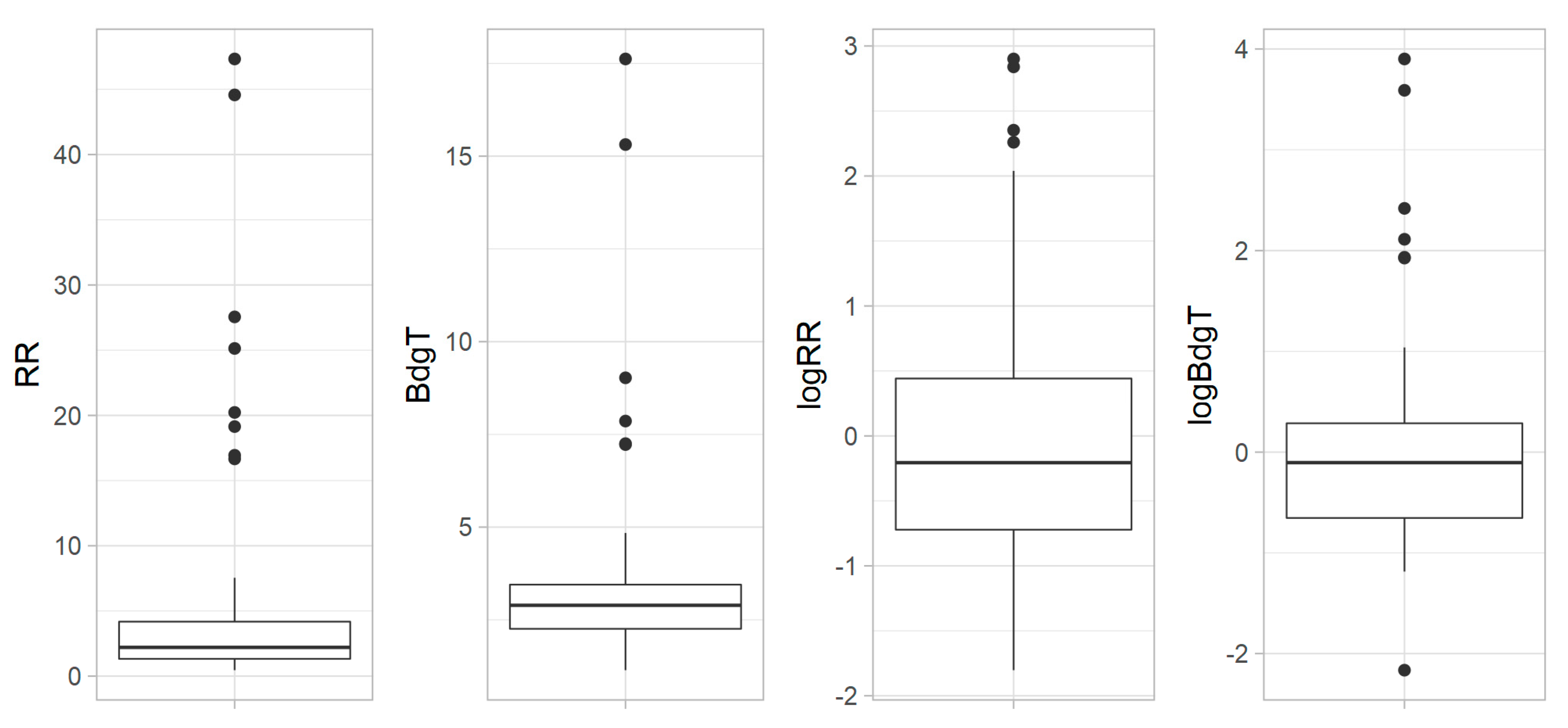
Most RR values ranged between 0.46 and 7.55 µmol O2 h−1, though eight samples had higher values up to 47.3 µmol O2 h−1 (Figure 4). Similarly, most BdgT values ranged from 1.14 h to 4.84 h, with outliers as high as 17.6 h. As is evident from Figure 5, the RR and BdgT data were not normally distributed, but skewed towards higher values. The data were thus log transformed for the following analysis.
The respiration rate (RR) and biodegradation period (BdgT) were calculated from the derivate of the O2 slope data. RR is not correlated to BdgT (confidence interval for R being (−0.25; 0.21)), indicating that RR and BdgT reflect different aspects of the microbial degradation process. An ANOVA showed that there was no significant difference between the three site clusters of bacterial composition (Section 2.3.3) and mean RR (p = 0.7) and BdgT (p = 0.9). The use of a non-indigenous inoculum does thus not appear to have affected the biodegradation parameters.
3.2. Covariation of Variables
A total of 27 potential explanatory parameters were selected from the CBA lake survey (see Section 2.2.). However, regression models are sensitive to collinearity between covariates. Therefore, a correlation matrix with Pearson correlation coefficients was calculated for the 27 potential explanatory variables. The full matrix is presented in the Supplementary Material (Part D Figure S2). Only covariates with a correlation coefficient lower than 0.5 were kept, in order to avoid interaction effects in the models. The resulting 12 selected explanatory parameters are presented in Table 2 and a correlation matrix with the log transformed response variables is presented in Figure 5.
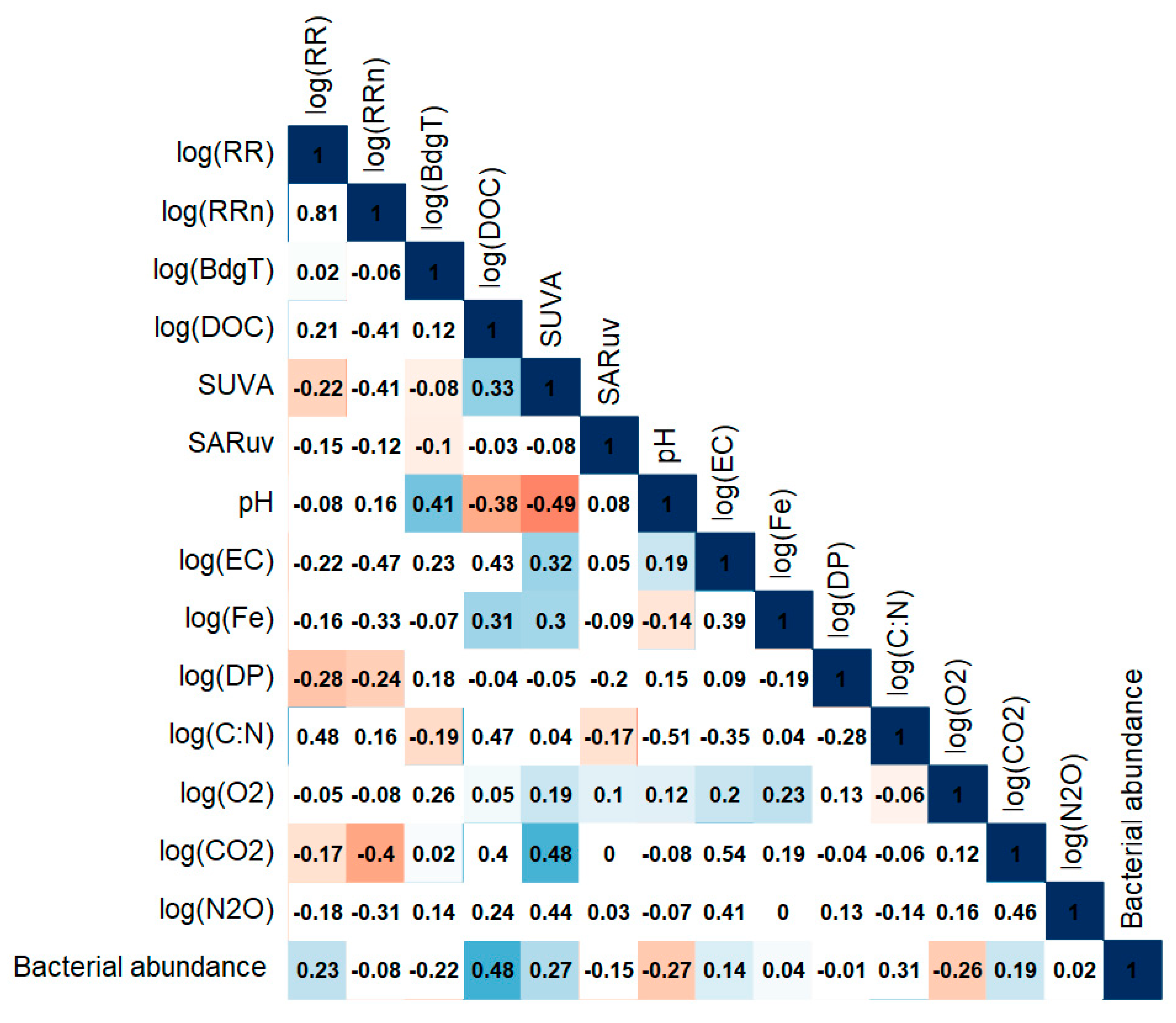
Log(RR) is significantly correlated (p-value < 0.05) with sUVa (r = −0.22), log(DP) (−0.28), log(CO2) (−0.17), and cells counts (0.23) (Figure 5). It is also strongly, though not significantly, correlated with log(C:N). The correlation coefficient between log(RRn) and log(RR) is high (r = 0.81), although the p-value is higher than 0.05. Therefore, this correlation is not significant. Log(RR) has negative significant correlations with log(DP) (r = −0.24) and log(CO2) (r = −0.4). Log(BdgT) is not correlated with log(RR) or log(RRn), but is significantly correlated with pH (r = 0.41) and log(C:N) (r = −0.19). It has also weak significant correlations with sUVa and SARuv (r = −0.08 and r = −0.1).
3.3. Selection of Drivers of Biodegradability
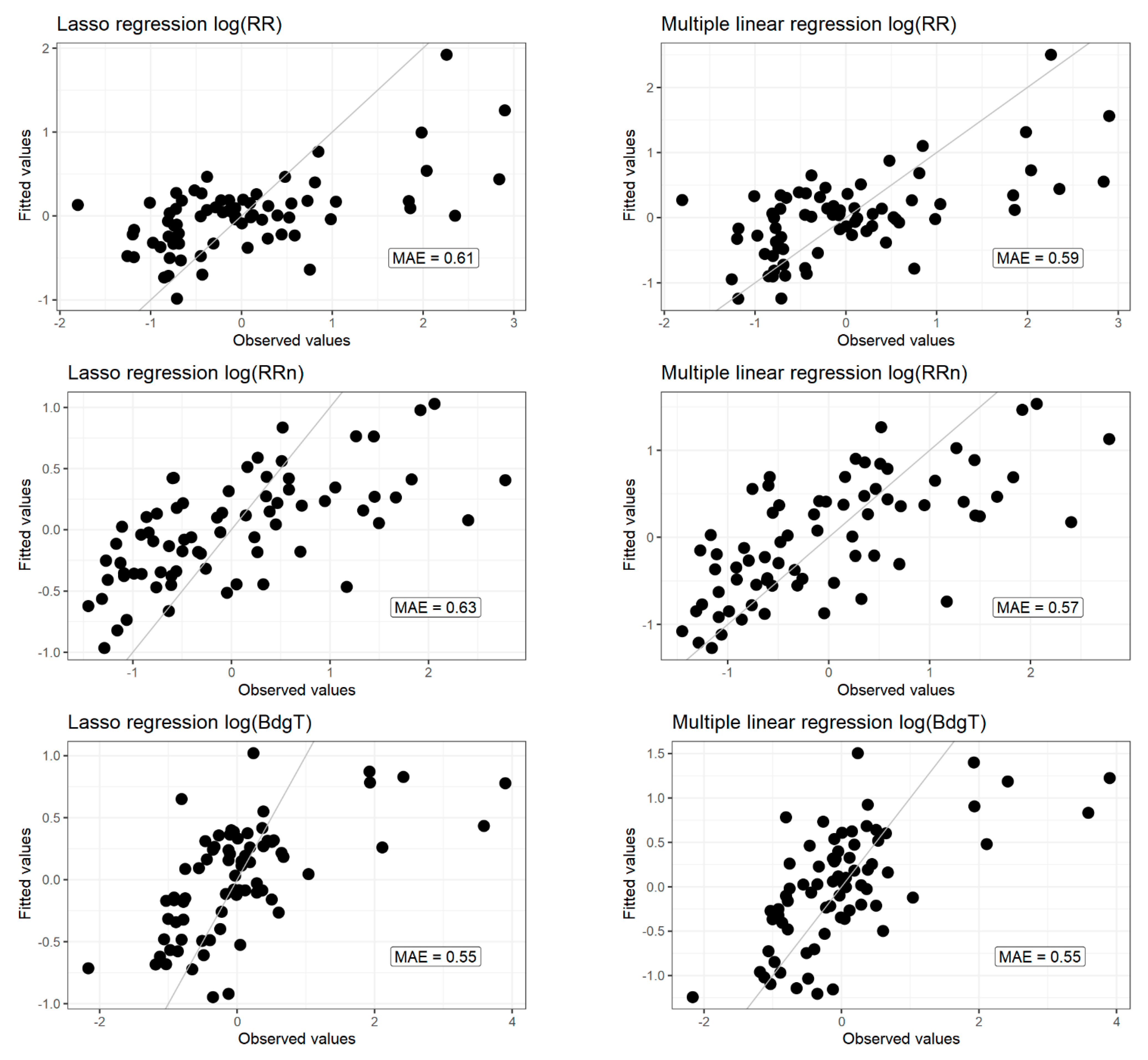
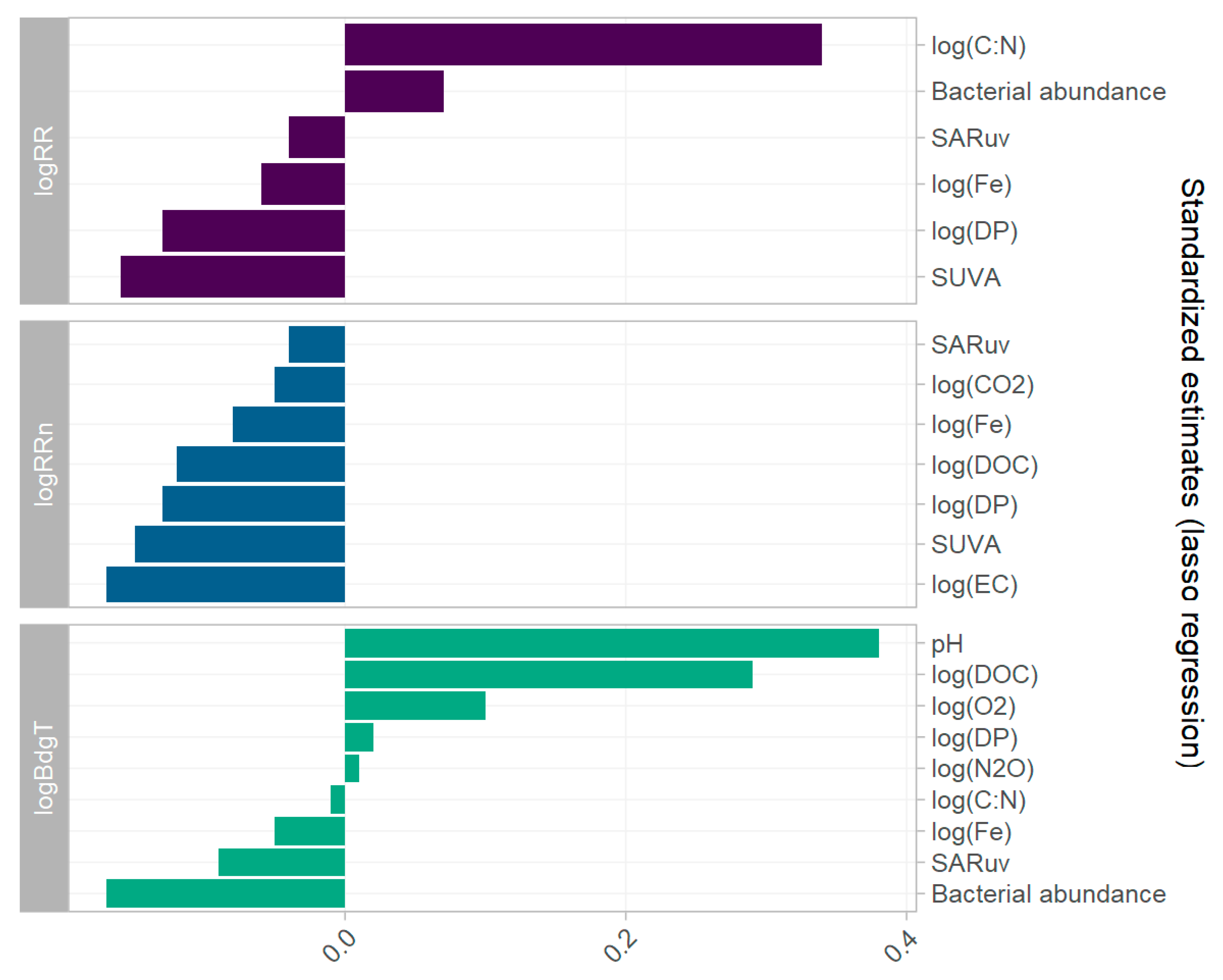
Lasso multiple linear regressions were applied to the dataset of 12 selected explanatory parameters (Table 2) for each of the three log transformed response variables. The lasso regression is a statistical tool allowing covariates with little explanatory power to be discarded, thus only keeping significant covariates. The fitted vs. observed values of the multiple linear regression models are plotted in Figure 6. Their performances are presented by residual plots in the Supplementary Material (Part E Figures S7–S9). The mean absolute error of each of the models was low, but the normal Q-Q plots display residuals skewed to the right, and not following the normal distribution. The estimates for each lasso regression model are plotted in Figure 7.
The lasso regression model with log(RR) as response variable selected six covariates of the 12 (Table 2). Because the dataset was standardised, the estimates reflect the effect size of each variable, not the absolute effect. Log(C:N) was the parameter with the highest explanatory value on log(RR) with β = 0.34. On the contrary, the estimate for log(DP) was β = −0.13. Nutrient concentrations were based on the concentration in the original sample, before addition of nutrients for the incubation experiment. Log(RR) was thus found to increase with an increasing original C:N ratio, and decrease with increasing original DP concentration. sUVa also had a high explanatory value with β = −0.16. (RRn). Cells count, log(Fe), and SARuv were also selected by the model, with estimates of β = 0.07, β = −0.06, and β = −0.04, respectively.
For the modelling of log(RRn), seven covariates were selected by the lasso regression, all with a negative effect. Log(EC) had the largest effect with β = −017, followed by sUVa with −0.15. Moreover, log(DP), log(DOC), and log(Fe) had negative estimates, in addition to log(CO2) and log(SARuv) (β = −0.13, −0.12, −0.06, and −0.05 and −0.04 respectively). This suggests that the normalised respiration rate (the respiration rate divided by the organic carbon concentration) decreases with increasing DOC and phosphate concentrations, and with increasing conductivity (a proxy for ionic strength).
Of the 12 selected covariates, nine were selected for log(BdgT). The estimates with the highest coefficients were the pH with β = 0.38, followed by log(DOC) with β = 0.29, and log(O2) with β = 0.10. Cells count and SARuv had a negative effect on log(BdgT), with β = 0.17 and β = 0.09, respectively. Log(DP), log(N2O), log(C:N), and log(Fe) were also selected but had minor effects (β being 0.02, 0.01, −0.01, and −0.05, respectively). The effect of the nutrient concentration on log(BdgT) was opposite to the one observed for log(RR).
3.4. Significance of the Selected Drivers of Biodegradabilityz
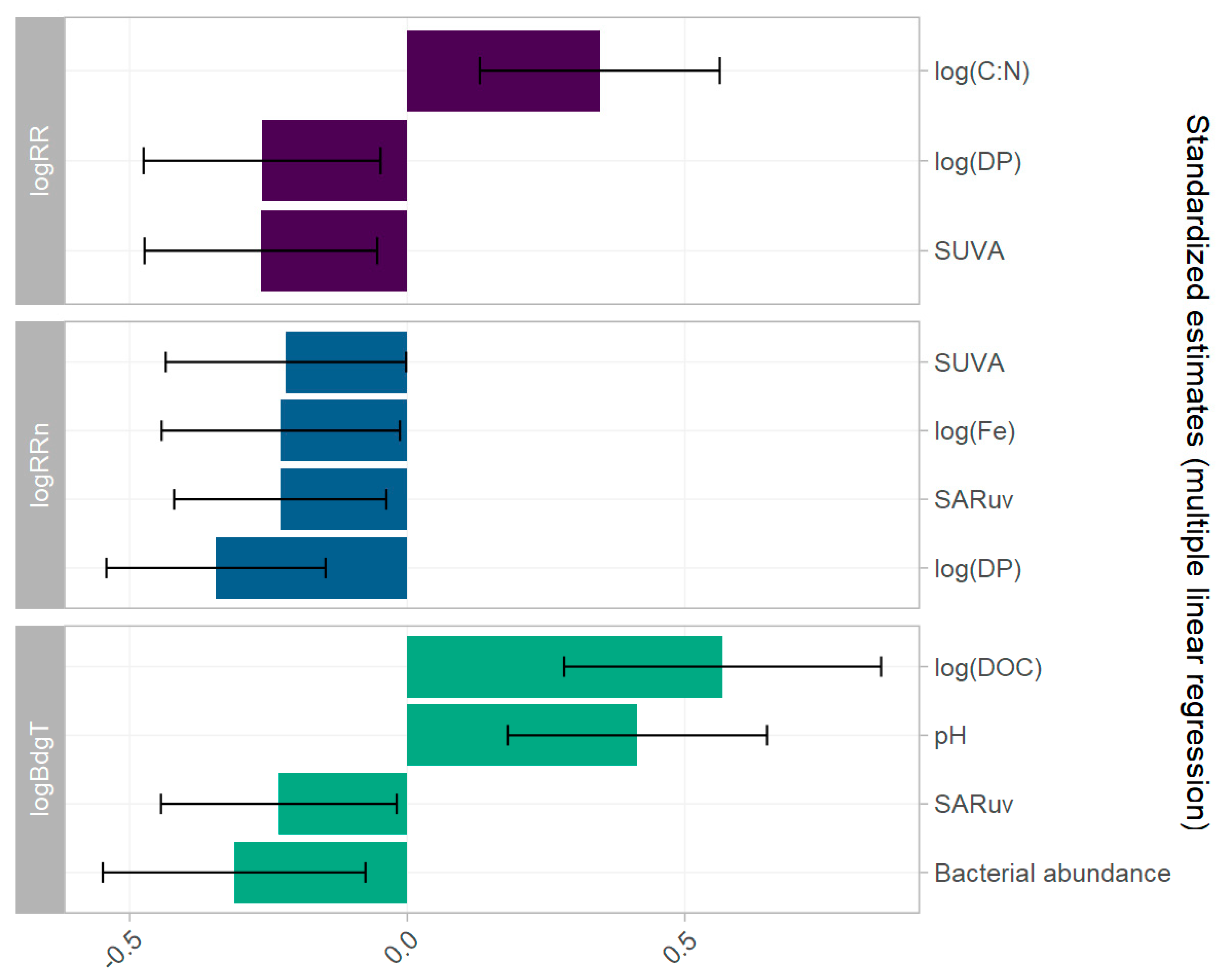
Multiple linear regression models for each of the three variables describing the biodegradability of DNOM were constructed based on only the explanatory variables selected by lasso regression (Section 3.3). Each model was performed on the 50 imputed datasets and the resulting estimates, residuals, and predicted values were pooled. The fitted vs. observed values are represented in Figure 7. The residual plots of the model are presented in the Supplementary Material (Part F Figures S10–S12).
The mean absolute errors of the models are similar to those obtained with the lasso regression. Despite the log transformation, residuals are skewed to the right and there is still heteroscedasticity of the data. Moreover, certain data points had high leverage in the model, but no lake had both high leverage and high studentised residual (>3), so all the points were retained in the model. Estimates for the covariates are represented for each model in Figure 8. Only the significant estimates with a p-value less than 0.05 are represented (Supplementary Material Part F Table S3). Compared to the lasso regression, few covariates remained significant.
Log(RR) is exclusively dependent on sUVa, log(C:N), and log(DP), with log(C:N) remaining as the predictor with the highest impact (β = 0.35), followed by sUVa and log(DP), both with β = −0.26.
Log(RRn) is negatively impacted by sUVa and log(DP) in a similar manner as log(RR), with β = −0.22 and −0.34, respectively. In addition, log(Fe) and SARuv had equally important effects (β = −0.23). Four explanatory variables were kept for log(BdgT): log(DOC), pH, SARuv, and Cells count (i.e., bacterial abundance) with respective estimates of 0.57, 0.41 and −0.23, and −0.31.
4. Discussion
4.1. Priming Effect Boosting the Respiration Rate
The specific UV absorbance (sUVa) had an explanatory value for the observed variation of log(RR) and log(RRn), both in the correlation analysis and in the lasso and multiple linear regressions. A high sUVa value is an indicator of HMW and of a high degree of aromaticity of the DNOM [36]. Several authors have shown that DNOM with a low sUVa is preferably degraded compared to DNOM with a high sUVa. For example, Zhou et al. [41] highlighted a negative correlation between the BDOM and the sUVa value, and Abbott et al. [42] showed that the sUVa increases during the first 10 days of an incubation experiment, meaning that the HMW aromatic compounds were less degraded than the LMW saturated moieties. Our incubation experiment, focusing on the first hours of bacterial decomposition of the DNOM, confirms that bacterial communities consume preferentially the LMW and more saturated moieties of the DNOM pool. Even if the residence time of the water in the studied lakes can extend up to 8 years [43] (as represented by Mjøsa, Norway’s largest lake), the bacterial community will prioritise fresh, light moieties of DNOM over the remaining HMW compounds. The log normalised respiration rate (log(RRn)) was also negatively associated with sUVa in the lasso and multiple linear regression models, although this relationship may be inherent because both variables are derived by dividing by DOC. Log(Fe) was also found to have a slight negative explanatory value on log(RR) and log(RRn). Practically all Fe in these generally oxic surface waters is complexed to the DNOM. Typically, the HMW moieties of the DNOM have higher Fe content [44,45]. The role of log(Fe) as an explanatory factor for log(RR) and log(RRn) may thus reflect a covariation to the larger size of the DNOM, and thereby lower biodegradability, as reflected by sUVa (r = 0.3, Figure 6).
Although the log(C:N) ratio was not significantly correlated with log(RR) (Figure 6), it excelled as an explanatory predictor, both in the lasso and in the multiple linear regression models of log(RR) (Figure 7 and Figure 8). The C:N ratio was calculated as the molar ratio of DOC/DN, both DOC and DN being measured in filtered water (0.45 um). In the assessed lake water samples, it displayed a pronounced variation, ranging from 9.33 to 450, with a mean of 49.0. This greatly exceeds the Redfield ratio observed in marine phytoplankton cells (the molar Redfield ratio for C:N being 6.6), which would be assumed to represent the C:N ratio of algae-derived, autochthonous DOM. Large deviations from this stoichiometry are commonly observed in inland waters [46,47] and oceans [48]. The relatively high C:N ratio indicates recalcitrant, terrestrially derived organic matter, potentially already partially degraded by a microbial community, contrary to autochthonous and algae-derived DNOM [49,50]. N-poor DNOM implies that proteins and amino acids are depleted, yielding low-quality DNOM for bacterial consumption. This is due to the large import of allochthonous DNOM [51] to surface waters in the boreal biome, and the long residence time in the lake [52]. In addition, the degradation of the most recalcitrant moieties of DNOM may primarily be restricted by the N limitation [37]. Therefore, the addition of nutrients in our incubation experiment might have led to a “priming effect”, making the relatively LMW and more saturated DNOM moieties with a high C:N ratio available for microbial degradation. Such a priming effect occurs naturally in boreal lakes, for instance, during seasonal turnovers, when the water from the hypolimnion is mixed with the nutrient-depleted water of the epilimnion [53].
The respiration rate was also partly explained by log(DP), which was negatively correlated with log(RR) (r = −0.28, Figure 6) and had a negative impact in the lasso and multiple linear regression models (Figure 7 and Figure 8). Abbott et al. [54] found that DP in their permafrost leachate samples was a good positive indicator of the percentage of BDOC. Similarly, Allesson et al. [18] reported a higher turnover of BDOM in lakes in which P was in surplus. In our incubation experiment, all treatments received N and P to avoid the effects of nutrient limitation, in order to specifically test the role of DNOM quality on respiration. Nonetheless, the negative effect of log(DP) appears counterintuitive but may be because, in more nutrient-rich systems, the available DNOM was previously degraded. This supports the hypothesis of the priming effect in nutrient-poor samples.
4.2. Slower Biodegradation in Autotrophic Lakes
Log(BdgT) was positively associated with log(DOC) in the lasso and linear regressions (Figure 7 and Figure 8). This is an inherent baseline condition for the biodegradation: the more DNOM and thereby BDOM to degrade, the longer the biodegradation period. However, log(BdgT) was negatively correlated with log(C:N) (Figure 6), which suggests a longer biodegradation time for labile DNOM. A possible explanation for this apparent contradiction is that the bacterial community faces a more heterogeneous pool of BDOM in lakes with a higher share of labile DNOM.
This is supported by the association between the biodegradation period (BdgT) and autotrophic conditions. First, log(O2) appeared as the main explanatory positively correlated variable in the lasso regression for log(BdgT) (Figure 8). High oxygen concentrations are common in the epilimnion of autotrophic lakes where the primary production releases dissolved oxygen in the layer of photosynthesis active radiation (PAR) [55]. As the samples in this study were collected from the surface, elevated O2 concentration likely indicates high primary production in the raw water. The positive effect of log(DP) and the negative effect of log(C:N) in the lasso regression (Figure 8) also support this hypothesis. In addition, pH was a positive explanatory factor for BdgT in the lasso and multiple linear regression (Figure 7 and Figure 8). It was itself positively related to log(Alkalinity) and log(Ca) (Table 2). Typically, these lakes are eutrophic with an inherent significant production of autochthonous BDOM [56,57].
As shown above, lighter BDOM is degraded preferentially even though the nutrient limitation is removed. Therefore, in lakes comprising both autochthonous and allochthonous DNOM, the biodegradation phase lasts longer because both the light BDOM and the less recalcitrant share of allochthonous DNOM are degraded by the bacterial community.
4.3. Enhanced Bacterial Respiration in Dystrophic Lakes
The speed and duration of respiration by the bacterial community was measured, assuming that for one molar unit of oxygen gas consumed, the bacterial community consumed one molar unit of carbon. However, this is based on the theorical value for glucose degradation. In reality, the degradation of compounds of lower molecular weight, containing more oxygen, could yield an RQ well above 1 [17,58]. In this case, the respiration of DNOM with a large share of autochthonous, light DNOM would be underestimated by controlling only the oxygen consumption. The higher respiration rate in samples from dystrophic lakes may reflect a RQ closer to 1, contrarily to the respiration rate in samples from mesotrophic lakes, where more autochthonous DNOM is available.
In addition, the microbial fixation of DNOM was not measured. The actual concurrence of these two processes can also explain the behaviour of the bacterial community in meso/eutrophic lakes and in dystrophic lakes, with a longer biodegradability lapse in the former and a higher respiration rate in the latter. Indeed, community respiration reflects both the cell-specific and the overall heterotrophic community activity. Situations with “excess C” may yield high cell-specific respiration (typically high RR), whereas higher levels of nutrients may lead to reduced cell-specific respiration, although with increased bacterial biomass and thus increased overall respiration (high BdgT) [59].
Abbott et al. [42] observed that, in samples with higher inorganic nitrogen concentration, a larger proportion of the DNOM was mineralised after the nutrient addition. They suggested that nutrient addition enhances preferentially the complete degradation of labile organic matter to CO2, rather than causing a priming effect by making recalcitrant organic matter available. In that case, high RR is a means for the microorganisms to spend excess C [59,60,61,62], thereby lowering the C:N ratio. This is supported by the fact that log(RR) and log(RRn) were negatively associated with proxies indicating higher nutrient lake status. First, log(RR) and log(RRn) were both negatively correlated with log(CO2) (Figure 6). Low CO2 concentrations are usually associated with autotrophic lakes, due to the autotrophic fixation of the CO2 [63]. Secondly, log(RRn) was negatively associated with log(EC) in the lasso regression (Figure 8). Log(EC) is a proxy of the trophic state because it is correlated with the ionic strength. Indeed, most eutrophic lakes are found in agricultural regions that are located below the marine limit with elevated levels of HCO3, Ca, Na and Cl, in addition to DP. Moreover, few dystrophic lakes have high levels of inorganic ions [64].
This is consistent with the findings of Allesson et al. [18], who also suggested that at a community level, bacterial production increases relative to the bacterial respiration in nutrient-rich lakes. We thus suggest that in meso- and eutrophic lakes, the bacterial community uses a large proportion of the DNOM to grow and respire, although only a small part is used to provide energy for this growth. Meso- and eutrophic lakes contain a high share of autochthonous, labile DNOM, which can be directly used for anabolism. This causes the bacterial community to use the available oxygen at a slower pace, and for a longer time. On the contrary, in dystrophic lakes, the bacterial community uses a larger proportion of the DNOM pool for respiration and a smaller part for assimilation, leading to high respiration rates and faster oxygen depletion.
5. Conclusions
We tested the applicability of an analytical method to determine the biodegradability of DNOM, based on the rate of oxygen consumption by bacteria during incubation under optimal conditions. The respiration rate (RR) and the DOC normalized RR (RRn), in addition to the duration of rapid biodegradation (BdgT) of the DNOM, showed significant spatial variation among boreal lakes in southeast Norway.
The variation in the RR was mainly driven by the characteristics of the DNOM. HMW and aromatic DNOM was respired more slowly than LMW and hydrogen saturated DNOM. Indeed, the sUVa was a main predictor of both the RR and RRn. The RR was also governed by the trophic state of the lake. However, dystrophic lakes, with a high proportion of recalcitrant DNOM and a low nutrient concentration, had the highest RR. It is likely that the amount of BDOM left in these dystrophic lake water samples is low due to the long residence time of lake water. It is thus hypothesised that the high RR is due to a priming effect, caused by the addition of nutrients for the incubation experiment. Because the studied lakes are generally lower-mesotrophic and dystrophic, the addition of nitrogen and phosphate allowed an increased respiration rate. This implies that the rate of heterotrophic respiration in these nutrient-poor lakes is mainly governed by the availability of reactive nutrients and, in particular, nitrogen, with the C:N ratio being a main predictor of the respiration rate.
Nutrient-rich lakes with high pH and oxygen concentration displayed a longer BdgT. These lakes are also prone to contain more autochthonous DNOM, which is generally more readily biodegradable. This suggests that the longer biodegradation period reflects a greater variety in the DNOM quality, due to a mix of autochthonous and allochthonous organic matter, which forces the bacteria community to adjust and thus extend its growth phase. Although the RR is faster for lakes with a higher proportion of labile organic matter, the biodegradation period may last longer due to the larger heterogeneity of the biodegradable matter, in addition to a greater quantity of BDOM to degrade.
Our findings suggest that the balance between rapid RR and long BdgT may be partly governed by the balance between bacterial respiration and assimilation. A DNOM pool with a lower proportion of labile nutrient compounds (i.e., high C:N), such as in dystrophic lakes, would enhance the bacterial respiration, hence resulting in a faster RR. On the contrary, a DNOM pool with a high proportion of bioavailable autochthonous compounds, such as those found in eutrophic lakes, would be better suited for bacterial assimilation, hence leading to a longer biodegradation duration.
Supplementary Materials
The following are available online at https://www.mdpi.com/article/10.3390/w13162210/s1: Figure S1: Repartition of the 73 lakes depending on their trophic state, based on Carlson’s Trophic State Index; Figure S2: Organization of a sensor plate. Figure; S3: Snapshot of the SDS interface; Figure S4: Example of the oxygen concentration in a natural lake water sample; Figure S5: Multiple imputation process; Figure S6: Correlation plot the 27 covariates; Figure S7: Residual plots for lasso regression with log(RR) as response variable; Figure S8: Residual plots for lasso regression with log(RRn) as response variable; Figure S9: Residual plots for lasso regression with log(BdgT) as response variable; Figure S10: Residual plots for linear model with log(RR) as response variable; Figure S11: Residual plots for linear model with log(RRn) as response variable; Figure S12: Residual plots for linear model with log(BdgT) as response variable; Table S1: Summary of the dataset from the CBA 100 lakes survey; Table S2: Lasso regression estimates (pooled for n > 25); Table S3: Linear model estimates and p-values (pooled for n > 25).
Author Contributions
Conceptualization, R.D.V., D.O.H. and C.C.; methodology, R.D.V. and C.C.; formal analysis, C.C. and T.A.; investigation, C.C. and N.V.; data curation, C.C. and N.V.; writing—original draft preparation, C.C.; writing—review and editing, R.D.V., D.O.H., T.A. and N.V.; visualization, C.C.; supervision, R.D.V., D.O.H. and T.A.; project administration, R.D.V. All authors have read and agreed to the published version of the manuscript.
Funding
This research was funded by the Center of Biogeochemistry in the Anthropocene (University of Oslo).
Institutional Review Board Statement
Not applicable.
Informed Consent Statement
Not applicable.
Data Availability Statement
The data used in this study is available on the open access repository Open Science Forum, to any person with a user account. https://osf.io/r39ng/?view_only=e9a3b3de84794bfc9883db481cb9a483 (accessed on 17 July 2021). The R code written for this study is published on Github and freely available: https://github.com/CamilMC/100_lakes_2019 (accessed on 17 July 2021).
Acknowledgments
We thank all of the participants of the CBA-100 lakes survey, who took part in the sampling of the lakes presented in this article. Eline Mosleth Fægerstad and Ragna Othilie Lie contributed significantly to the incubation experiment. Per-Johan Færøvig provided additional Presens sensors. Alexander Eiler and Laurent Fontaine developed the pipeline for amplicon analysis and Jing Wei undertook the microbial DNA extraction.
Conflicts of Interest
The authors declare no conflict of interest.
References
- Hessen, D.; Andersen, T.; Lyehe, A. Carbon metabolism in a humic lake: Pool sires and cycling through zooplankton. Limnol. Oceanogr. 1990, 35, 84–99. [Google Scholar] [CrossRef]
- Garmo, Ø.A. Trends and Patterns in Surface Water Chemistry in Europe and North America between 1990 and 2016, with Particular Focus on Changes in Land Use as a Confounding Factor for Recovery; NIVA REPORT SNO 7556-2020; The Norwegian Institute for Water Research: Oslo, Norway, 2020. [Google Scholar]
- Tranvik, L.J.; Downing, J.A.; Cotner, J.; Loiselle, S.; Striegl, R.G.; Ballatore, T.J.; Dillon, P.; Finlay, K.; Fortino, K.; Knoll, L.B.; et al. Lakes and reservoirs as regulators of carbon cycling and climate. Limnol. Oceanogr. 2009, 54, 2298–2314. [Google Scholar] [CrossRef] [Green Version]
- Larsen, S.; Andersen, T.; Hessen, D.O. Predicting organic carbon in lakes from climate drivers and catchment properties. Glob. Biogeochem. Cycles 2011, 25. [Google Scholar] [CrossRef]
- Finstad, A.G.; Andersen, T.; Larsen, S.; Tominaga, K.; Blumentrath, S.; A de Wit, H.; Tømmervik, H.; Hessen, D.O. From greening to browning: Catchment vegetation development and reduced S-deposition promote organic carbon load on decadal time scales in Nordic lakes. Sci. Rep. 2016, 6, 31944. [Google Scholar] [CrossRef] [Green Version]
- Mattsson, T.; Kortelainen, P.; Räike, A. Export of DOM from Boreal Catchments: Impacts of Land Use Cover and Climate. Biogeochemistry 2005, 76, 373–394. [Google Scholar] [CrossRef]
- De Wit, H.A.; Palosuo, T.; Hylen, G.; Liski, J. A carbon budget of forest biomass and soils in southeast Norway calculated using a widely applicable method. For. Ecol. Manag. 2006, 225, 15–26. [Google Scholar] [CrossRef]
- Sawicka, K.; Rowe, E.C.; Evans, C.D.; Monteith, D.T.; Vanguelova, E.I.; Wade, A.J.; Clark, J.M. Modelling impacts of atmospheric deposition and temperature on long-term DOC trends. Sci. Total Environ. 2017, 578, 323–336. [Google Scholar] [CrossRef] [Green Version]
- De Wit, H.A.; Mulder, J.; Hindar, A.; Hole, L. Long-Term Increase in Dissolved Organic Carbon in Streamwaters in Norway Is Response to Reduced Acid Deposition. Environ. Sci. Technol. 2007, 41, 7706–7713. [Google Scholar] [CrossRef] [PubMed]
- Thrane, J.-E.; Hessen, D.O.; Andersen, T. The Absorption of Light in Lakes: Negative Impact of Dissolved Organic Carbon on Primary Productivity. Ecosystems 2014, 17, 1040–1052. [Google Scholar] [CrossRef] [Green Version]
- Yang, H.; Andersen, T.; Dörsch, P.; Tominaga, K.; Thrane, J.-E.; Hessen, D.O. Greenhouse gas metabolism in Nordic boreal lakes. Biogeochemistry 2015, 126, 211–225. [Google Scholar] [CrossRef] [Green Version]
- Rajakumar, J. Effect of Photo-Oxidation on Size, Structure and Biodegradability of Dissolved Natural Organic Matter. Master’s Thesis, University of Oslo, Oslo, Norway, 2018. [Google Scholar]
- Liu, S.; He, Z.; Tang, Z.; Liu, L.; Hou, J.; Li, T.; Zhang, Y.; Shi, Q.; Giesy, J.P.; Wu, F. Linking the molecular composition of autochthonous dissolved organic matter to source identification for freshwater lake ecosystems by combination of optical spectroscopy and FT-ICR-MS analysis. Sci. Total Environ. 2020, 703, 134764. [Google Scholar] [CrossRef] [PubMed]
- Hansen, A.M.; Kraus, T.; Pellerin, B.; Fleck, J.A.; Downing, B.; Bergamaschi, B. Optical properties of dissolved organic matter (DOM): Effects of biological and photolytic degradation. Limnol. Oceanogr. 2016, 61, 1015–1032. [Google Scholar] [CrossRef] [Green Version]
- Marschner, B.; Kalbitz, K. Controls of bioavailability and biodegradability of dissolved organic matter in soils. Geoderma 2003, 113, 211–235. [Google Scholar] [CrossRef]
- Brown, D.M.; Hughes, C.B.; Spence, M.; Bonte, M.; Whale, G. Assessing the suitability of a manometric test system for determining the biodegradability of volatile hydrocarbons. Chemosphere 2018, 195, 381–389. [Google Scholar] [CrossRef]
- Allesson, L.; Ström, L.; Berggren, M. Impact of photochemical processing of DOC on the bacterioplankton respiratory quotient in aquatic ecosystems. Geophys. Res. Lett. 2016, 43, 7538–7545. [Google Scholar] [CrossRef] [Green Version]
- Allesson, L.; Andersen, T.; Dörsch, P.; Eiler, A.; Wei, J.; Hessen, D.O. Phosphorus Availability Promotes Bacterial DOC-Mineralization, but Not Cumulative CO2-Production. Front. Microbiol. 2020, 11. [Google Scholar] [CrossRef]
- Håland, A. Characteristics and Bioavailability of Dissolved Natural Organic Matter in a Boreal Stream during Storm Flow. Master’s Thesis, University of Oslo, Oslo, Norway, 2017. [Google Scholar]
- Færgestad, E.M. Biodegradability and Spectroscopic Properties of DNOM Affected by Mercury Transport and Uptake. Master’s Thesis, University of Oslo, Oslo, Norway, 2019. [Google Scholar]
- Henriksen, A.; Brit, L.S.; Jaakko, M. Results of National Lake Surveys 1995 in Finland, Norway, Sweden, Denmark, Russian Kola, Russian Karelia, Scotland and Wales; Technical Report; U.S. Department of Energy: Washington, DC, USA, 1997.
- Henriksen, A.; Brit, L.S.; Jaakko, M.; Anders, W.; Ron, H.; Chris, C.; Jens, P.J.; Erik, F.; Tatyana, M. Northern European Lake Survey 1995: Finland, Norway, Sweden, Denmark, Russian Kola, Russian Karelia, Scotland and Wales. Ambio 1998, 27, 80–91. [Google Scholar]
- Crapart, C.; Parra, N. CBA 100 Lakes. Available online: https://osf.io/r39ng/?view_only=e9a3b3de84794bfc9883db481cb9a483 (accessed on 17 July 2021).
- Åberg, J.; Wallin, M. Evaluating a fast headspace method for measuring DIC and subsequent calculation of pCO2 in freshwater systems. Inland Waters 2014, 4, 157–166. [Google Scholar] [CrossRef]
- Schielzeth, H. Simple means to improve the interpretability of regression coefficients. Methods Ecol. Evol. 2010, 1, 103–113. [Google Scholar] [CrossRef]
- Biodegradability of DNOM. Available online: https://www.protocols.io/view/biodegradability-of-dnom-biyykfxw (accessed on 2 August 2020).
- Gjessing, E.; Egeberg, P.; Håkedal, J. Natural organic matter in drinking water ? The ?NOM-typing project?, background and basic characteristics of original water samples and NOM isolates. Environ. Int. 1999, 25, 145–159. [Google Scholar] [CrossRef]
- Najafpour, G.D. Growth Kinetics. In Biogeochemical Engineering and Biotechnology; Elsevier B.V.: Amsterdam, The Netherlands, 2017; pp. 81–141. [Google Scholar]
- Langenheder, S.; Lindström, E.; Tranvik, L.J. Weak coupling between community composition and functioning of aquatic bacteria. Limnol. Oceanogr. 2005, 50, 957–967. [Google Scholar] [CrossRef] [Green Version]
- Comeau, A.M.; Douglas, G.M.; Langille, M.G.I. Microbiome Helper: A Custom and Streamlined Workflow for Microbiome Research. mSystems 2017, 2, e00127-16. [Google Scholar] [CrossRef] [PubMed] [Green Version]
- Martin, M. Cutadapt removes adapter sequences from high-throughput sequencing reads. EMBnet. J. 2011, 17, 10–12. [Google Scholar] [CrossRef]
- Callahan, B.J.; McMurdie, P.J.; Rosen, M.J.; Han, A.W.; Johnson, A.J.A.; Holmes, S.P. DADA2: High-resolution sample inference from Illumina amplicon data. Nat. Methods 2016, 13, 581–583. [Google Scholar] [CrossRef] [PubMed] [Green Version]
- Charrad, M.; Ghazzali, N.; Boiteau, V.; Niknafs, A. Nbclust: An R package for determining the relevant number of clusters in a data set. J. Stat. Softw. 2014, 61, 1–36. [Google Scholar] [CrossRef] [Green Version]
- Kassambara, A.; Mundt, F. Factoextra: Extract and Visualize the Results of Multivariate Data Analyses. Available online: https://cran.r-project.org/package=factoextra (accessed on 17 July 2021).
- Galili, T. dendextend: An R package for visualizing, adjusting and comparing trees of hierarchical clustering. Bioinformatics 2015, 31, 3718–3720. [Google Scholar] [CrossRef] [PubMed] [Green Version]
- Van Buren, S. Flexible Imputation of Missing Data; CRC Press: Boca Raton, FL, USA, 2018; Available online: https://stefvanbuuren.name/fimd/foreword.html (accessed on 8 February 2021).
- Zuur, A.F.; Ieno, E.N.; Elphick, C.S. A protocol for data exploration to avoid common statistical problems: Data exploration. Methods Ecol. Evol. 2010, 1, 3–14. [Google Scholar] [CrossRef]
- Casella, G.; Fienberg, S.; Olkin, I. An Introduction to Statistical Learning; Springer: New York, NY, USA, 2013. [Google Scholar]
- Boehmke, B.; Greenwell, B. Chapter 6 Regularized Regression. In Hands-On Machine Learning with R; CRC Press: Boca Raton, FL, USA, 2020; Available online: https://bradleyboehmke.github.io/HOML/regularized-regression.html (accessed on 7 April 2021).
- Ooi, H. Glmnetutils: Utilities for ‘Glmnet. 2021. Available online: https://cran.r-project.org/web/packages/glmnetUtils/index.html (accessed on 17 July 2021).
- Zhou, L.; Zhou, Y.; Tang, X.; Zhang, Y.; Jeppesen, E. Biodegradable dissolved organic carbon shapes bacterial community structures and co-occurrence patterns in large eutrophic Lake Taihu. J. Environ. Sci. 2021, 107, 205–217. [Google Scholar] [CrossRef]
- Toosi, E.R.; Clinton, P.W.; Beare, M.H.; Norton, D.A. Biodegradation of Soluble Organic Matter as Affected by Land-Use and Soil Depth. Soil Sci. Soc. Am. J. 2012, 76, 1667–1677. [Google Scholar] [CrossRef]
- NVE Temakart. Available online: https://temakart.nve.no/tema/innsjodatabase (accessed on 17 July 2021).
- Du, Y.; Ramirez, C.E.; Jaffé, R. Fractionation of Dissolved Organic Matter by Co-Precipitation with Iron: Effects of Composition. Environ. Process. 2018, 5, 5–21. [Google Scholar] [CrossRef]
- Xiao, Y.; Riise, G. Coupling between increased lake color and iron in boreal lakes. Sci. Total Environ. 2021, 767, 145104. [Google Scholar] [CrossRef]
- They, N.H.; Amado, A.M.; Cotner, J. Redfield Ratios in Inland Waters: Higher Biological Control of C:N:P Ratios in Tropical Semi-arid High Water Residence Time Lakes. Front. Microbiol. 2017, 8, 1505. [Google Scholar] [CrossRef] [PubMed] [Green Version]
- Andersen, T.; Hessen, D.O. Carbon, nitrogen, and phosphorus content of freshwater zooplankton. Limnol. Oceanogr. 1991, 36, 807–814. [Google Scholar] [CrossRef]
- Hopkinson, C.S.; Vallino, J. Efficient export of carbon to the deep ocean through dissolved organic matter. Nat. Cell Biol. 2005, 433, 142–145. [Google Scholar] [CrossRef] [PubMed]
- Kähler, P.; Koeve, W. Marine dissolved organic matter: Can its C:N ratio explain carbon overconsumption? Deep. Sea Res. Part I Oceanogr. Res. Pap. 2001, 48, 49–62. [Google Scholar] [CrossRef]
- Rantala, M.V.; Nevalainen, L.; Rautio, M.; Galkin, A.; Luoto, T.P. Sources and controls of organic carbon in lakes across the subarctic treeline. Biogeochemistry 2016, 129, 235–253. [Google Scholar] [CrossRef]
- Sepp, M.; Kõiv, T.; Nõges, P.; Nõges, T. The role of catchment soils and land cover on dissolved organic matter (DOM) properties in temperate lakes. J. Hydrol. 2019, 570, 281–291. [Google Scholar] [CrossRef]
- Jonsson, A.; Algesten, G.; Bergström, A.-K.; Bishop, K.; Sobek, S.; Tranvik, L.J.; Jansson, M. Integrating aquatic carbon fluxes in a boreal catchment carbon budget. J. Hydrol. 2007, 334, 141–150. [Google Scholar] [CrossRef]
- Bellido, J.L.; Peltomaa, E.; Ojala, A. An urban boreal lake basin as a source of CO2 and CH4. Environ. Pollut. 2011, 159, 1649–1659. [Google Scholar] [CrossRef] [PubMed]
- Abbott, B.W.; Larouche, J.R.; Jones, J.B.; Bowden, W.B.; Balser, A. Elevated dissolved organic carbon biodegradability from thawing and collapsing permafrost. J. Geophys. Res. Biogeosciences 2014, 119, 2049–2063. [Google Scholar] [CrossRef]
- Laas, A.; Cremona, F.; Meinson, P.; Rõõm, E.-I.; Nõges, T.; Nõges, P. Summer depth distribution profiles of dissolved CO2 and O2 in shallow temperate lakes reveal trophic state and lake type specific differences. Sci. Total Environ. 2016, 566–567, 63–75. [Google Scholar] [CrossRef]
- Ryder, R.A. The Morphoedaphic Index—Use, Abuse, and Fundamental Concepts. Trans. Am. Fish. Soc. 1982, 111, 154–164. [Google Scholar] [CrossRef]
- Cole, J.J.; Findlay, S.; Pace, M.L. Bacterial production in fresh and saltwater ecosystems: A cross-system overview. Mar. Ecol. Prog. Ser. 1988, 43, 1–10. [Google Scholar] [CrossRef]
- Berggren, M.; Lapierre, J.-F.; del Giorgio, P. Magnitude and regulation of bacterioplankton respiratory quotient across freshwater environmental gradients. ISME J. 2011, 6, 984–993. [Google Scholar] [CrossRef] [PubMed]
- Hessen, D.O.; Anderson, T.R. Excess carbon in aquatic organisms and ecosystems: Physiological, ecological, and evolutionary implications. Limnol. Oceanogr. 2008, 53, 1685–1696. [Google Scholar] [CrossRef]
- Jansson, M.; Bergström, A.-K.; Lymer, D.; Vrede, K.; Karlsson, J. Bacterioplankton Growth and Nutrient Use Efficiencies Under Variable Organic Carbon and Inorganic Phosphorus Ratios. Microb. Ecol. 2006, 52, 358–364. [Google Scholar] [CrossRef] [PubMed]
- Berggren, M.; Laudon, H.; Jansson, M. Landscape regulation of bacterial growth efficiency in boreal freshwaters. Glob. Biogeochem. Cycles 2007, 21. [Google Scholar] [CrossRef]
- Spohn, M. Microbial respiration per unit microbial biomass depends on litter layer carbon-to-nitrogen ratio. Biogeosciences 2015, 12, 817–823. [Google Scholar] [CrossRef] [Green Version]
- Balmer, M.B.; Downing, J.A. Carbon dioxide concentrations in eutrophic lakes: Undersaturation implies atmospheric uptake. Inland Waters 2011, 1, 125–132. [Google Scholar] [CrossRef]
- Tranvik, L.J. Dystrophy. In Encyclopedia of Inland Waters; Elsevier: Amsterdam, The Netherlands, 2009; pp. 405–410. [Google Scholar]
Figure 1.
Map of South Norway with the 73 sampled lakes and their DOC concentration (in mg/L) as a proxy for DNOM.
Figure 1.
Map of South Norway with the 73 sampled lakes and their DOC concentration (in mg/L) as a proxy for DNOM.

Figure 2.
Dendrogram of the 73 sampling sites sorted by similar bacteria classes. Different colours show the three main clusters. The inoculum was sampled in “Langtjern”. Computations were performed with the “factoextra” and “dendextend” packages in R.
Figure 2.
Dendrogram of the 73 sampling sites sorted by similar bacteria classes. Different colours show the three main clusters. The inoculum was sampled in “Langtjern”. Computations were performed with the “factoextra” and “dendextend” packages in R.

Figure 3.
Typical O2 concentration curve (top panel) and corresponding derivative (bottom panel). RR is the respiration rate and BdgT is the biodegradation Period (see Table 1).
Figure 3.
Typical O2 concentration curve (top panel) and corresponding derivative (bottom panel). RR is the respiration rate and BdgT is the biodegradation Period (see Table 1).

Figure 4.
Boxplots of respiration rate (RR) and biodegradability period (BdgT) and their log transformed data, showing the distribution of these parameters in the 73 sampled lakes. The line inside the box represents the median value, and the upper and lower sections of the box show the upper and lower quartiles. The whiskers represent 1.5 times the interquartile range. Outliers are marked as points outside the whiskers.

Figure 5.
Correlation plot of log transformed response variables log(RR), log(RRn), and log(BdgT), and the 12 selected explanatory variables. Blue and red coloured squares indicate positive and negative significant correlation coefficients (p < 0.05), respectively.
Figure 5.
Correlation plot of log transformed response variables log(RR), log(RRn), and log(BdgT), and the 12 selected explanatory variables. Blue and red coloured squares indicate positive and negative significant correlation coefficients (p < 0.05), respectively.

Figure 6.
Predicted vs. observed values for lasso regression and multiple linear regression.

Figure 7.
Estimates (pooled for n > 25) of parameter coefficients in lasso regression models of log(RR), log(RRn), and log(BdgT).
Figure 7.
Estimates (pooled for n > 25) of parameter coefficients in lasso regression models of log(RR), log(RRn), and log(BdgT).

Figure 8.
Estimates of the covariates in multiple linear regressions of log(RR), log(RRn), and log(BdgT). Error bars show the confidence interval for each estimate.
Figure 8.
Estimates of the covariates in multiple linear regressions of log(RR), log(RRn), and log(BdgT). Error bars show the confidence interval for each estimate.


Table 1.
Parameters describing the biodegradability of DNOM.
| Parameter | Definition | Interpretation |
|---|---|---|
| Maximum Respiration rate (RR) | Maximum biodegradation speed (µmolO2 L−1 h−1) | The maximum speed at which the microorganisms consume the DNOM, thus a proxy of the biodegradability of DNOM |
| Normalised respiration rate (RRn) | Respiration rate divided by the DOC (µmolO2 h−1 mgC−1) | The normalised respiration rate is a quality factor describing the relative speed of biodegradability, independent of the amount of DNOM. |
| Biodegradation period (BdgT) | Width of the half-peak (h) | The biodegradation period reflects the heterogeneity of DNOM quality, and balance of RR on the one hand and the amount of biodegradable matter on the other. |
Table 2.
Selected 12 explanatory parameter and their aliased covariates.
| Selected Explanatory Parameter | Aliased (Covariates with r > 0.5, p < 0.05 Are Indicated by an Asterisk (*)) | |
|---|---|---|
| Positive Correlations | Negative Correlations | |
| log(DOC) | log(C:P) *, SR, log(DN), log(B) | |
| sUVa | log(CH4) *, sVISa | |
| SARuv | None | |
| pH | log(Alkalinity) *, log(Ca) * | Log(Al) *, log(C:N) |
| log(EC) | log(Alkalinity) *, log(Ca) *, log(Mg) *, log(Na) *, log(SO4) *, log(Cl) *, log(B) *, log(DN) *, log(K), log(CO2) | |
| log(Fe) | None | |
| log(DP) | log(C:P) * | |
| log(C:N) | Log(C:P) | Log(SO4) *, log(DN) * |
| Log(O2) | log(T) * | |
| Log(CO2) | Log(EC), Log(B), log(CH4) | |
| Log(N2O) | sVISa | |
| Cells | None | |
Publisher’s Note: MDPI stays neutral with regard to jurisdictional claims in published maps and institutional affiliations. |
© 2021 by the authors. Licensee MDPI, Basel, Switzerland. This article is an open access article distributed under the terms and conditions of the Creative Commons Attribution (CC BY) license (https://creativecommons.org/licenses/by/4.0/).
Share and Cite
MDPI and ACS Style
Crapart, C.; Andersen, T.; Hessen, D.O.; Valiente, N.; Vogt, R.D. Factors Governing Biodegradability of Dissolved Natural Organic Matter in Lake Water. Water 2021, 13, 2210. https://doi.org/10.3390/w13162210
AMA Style
Crapart C, Andersen T, Hessen DO, Valiente N, Vogt RD. Factors Governing Biodegradability of Dissolved Natural Organic Matter in Lake Water. Water. 2021; 13(16):2210. https://doi.org/10.3390/w13162210
Chicago/Turabian StyleCrapart, Camille, Tom Andersen, Dag Olav Hessen, Nicolas Valiente, and Rolf David Vogt. 2021. "Factors Governing Biodegradability of Dissolved Natural Organic Matter in Lake Water" Water 13, no. 16: 2210. https://doi.org/10.3390/w13162210
Note that from the first issue of 2016, this journal uses article numbers instead of page numbers. See further details here.