
Performance of a Bog Hydrological System Dynamics Simulation Model in an Ecological Restoration Context: Soomaa Case Study, Estonia


1
Faculty of Engineering, Vidzeme University of Applied Sciences, Tērbatas iela 10, LV-4201 Valmiera, Latvia
2
Department of Geology, University of Tartu, 50090 Tartu, Estonia
*
Author to whom correspondence should be addressed.
Water 2021, 13(16), 2217; https://doi.org/10.3390/w13162217
Submission received: 30 June 2021
/
Revised: 6 August 2021
/
Accepted: 10 August 2021
/
Published: 14 August 2021
(This article belongs to the Section Ecohydrology)
Abstract
:We describe how a bog hydrology simulation model, developed in the System Dynamics environment, predicts the changes in the groundwater levels that result from drainage ditch closure and partial thinning of the surrounding forest stand. Five plots were selected in an area that was subjected to such ecological restoration, and the observed groundwater levels were compared with the simulated ones. Across the plots, the mean difference between the observed and simulated groundwater curves varied between 0.88 and 2.63 cm, and the RMSE between 0.28 and 0.71. Although the absolute difference between the predicted vs. observed values was greater in the plots with ditch closure, the curves co-varied more closely there over time. Therefore, hydrological System Dynamics models can be particularly useful for relative comparisons and risk-mapping of novel management scenarios.
1. Introduction
Investing in natural capital, including the restoration of carbon-rich habitats, is considered to be one of the five most important fiscal recovery policies that have a major economic multiplier effect and a positive impact on climate [1]. Mires cover 3% of the global land area, but accumulate about one-third of the soil carbon [2]. Intact mires are also habitats for many threatened species, regulate water and nutrient flows, and provide multiple cultural services to people across landscapes (e.g., [3]). By now, these functions have been greatly reduced in most regions with a long history of land use. Europe has lost more than 50% of its mires, with the largest losses in the past 75 years. Due to an emerging political consensus, substantial efforts of ecological restoration have been recently initiated within the EU to counteract such historical degradation [4]. From a global perspective, the United Nations recently launched its Decade on Ecosystem Restoration (2021–2030), focusing on mainstreaming ecological restoration in landscape contexts.
A necessity to understand how the mire ecosystems work, and what to expect in the case of human interventions, has been long acknowledged as a research priority [5,6]. For effective ecosystem restoration, it needs to be explicitly understood how, by changing one part of a mire, its other parts can be affected [7]. The groundwater level and its fluctuations are the key parameters for such understanding. There is an increasing need for reliable and feasible modelling tools for assessing the water supplies and wetland conditions, which could be then used as inputs for landscape and land-use planning. A desired feature of such modelling tools would be their robustness to specific land use practices, in order to predict the consequences of novel management regimes and the (expectably) unprecedented ecological restoration initiatives.
In boreal mires drained for forestry, the two main techniques for ecological restoration are thinning of the woody vegetation and ditch closure [8]. An explicitly described and tested model would be a valuable tool for planning these interventions at the ecosystem scale, given the conservation dilemmas and costs included [9]. The Regional Hydro-Ecological Simulation System (RHESSys) model predicts that forest thinning may cause an increase in annual streamflow, and watersheds that receive a higher rainfall have a more robust response; this supports tree thinning as a restoration option [10]. Hence, mire restoration planning requires a regional-scale model that explicitly and accurately includes the complex impacts of vegetation change on the water balance.
The existing applied models do not depict the restoration situations common in drained and afforested mires. For example, one of the most used hydrological models, MODFLOW, is designed to access the groundwater resources and does not include the vegetation parameters [11,12,13]. The Soil & Water Assessment Tool (SWAT) is a river basin-scale model used to simulate the quality and quantity of surface and groundwater and to predict the environmental impact of land use and management and climate change [14]; again, when the Green-Ampt infiltration equation is used to calculate infiltration in saturated soil, the interception of rainfall by the canopy must be calculated separately [15]. Several other hydrological models have been developed, such as WEAP [16], MIKE SHE [17], HecRAS [18], QUAL2K [19] and others, but their simplifications tend to allow reasonable accuracy only at large scales.
In order to accurately predict restoration and related impacts on individual mires, we have been developing a specific hydrological model in an environment of System Dynamics (SD), using the Stella Architect version 1.9.4, isee systems inc., Lebanon, PA, USA software. The central concept of the SD is understanding how all the objects in a system interact with one another through multiple feedback loops [20]. Previous hydrological models of bogs in the SD environment include the system dynamics watershed (SDW) model that lacked vegetation-related equations [21]. It was followed in 2009 by an improved version of the generic system dynamics watershed model (GSDW), which included interception and evaporation [22], but still did not show sufficient precision against field data [7]. The same study system (Gulbjusala bog in Latvia) was then used for a thorough revision and model simulation; the resulting equations, structure, and operating principles have been described in detail in a previous paper [23].
In the current phase of development, the work on the model has been continued with high-quality datasets from Estonia. A sensitivity analysis in an intact bog showed that transpiration had the greatest impact on the groundwater level. For groundwater fluctuations, the next most sensitive parameters were vegetation related: leaf area index (LAI), leaf distribution and inclination angle, and specific leaf area [24].
In this paper, we assess the performance of our SD model in a degraded bog forest that has been treated to recover its hydrological regime and, from a longer perspective, to restore its natural habitat conditions. Such an assessment (having the input data necessary) was possible in the protected Soomaa and Kikepera wetland complex in Estonia, where experimental mire restoration (in 2014–2015) has been accompanied with intensive pre- and post-treatment monitoring. The restoration included thinning of the forest cover (largely developed due to draining) and blocking ditches in various parts of the wetland that were separated from each other by forestry ditches. Our main study question is the parameter value of the LAI as a proxy to the vegetation effects. LAI is expressed as half of the sum of leaf areas per unit ground area [25]. LAI is strictly related to many ecological processes, such as transpiration, interception and carbon flux [26] and can indicate the growth status of forest vegetation [27].
2. Materials and Methods
2.1. Study Area and Test Plots
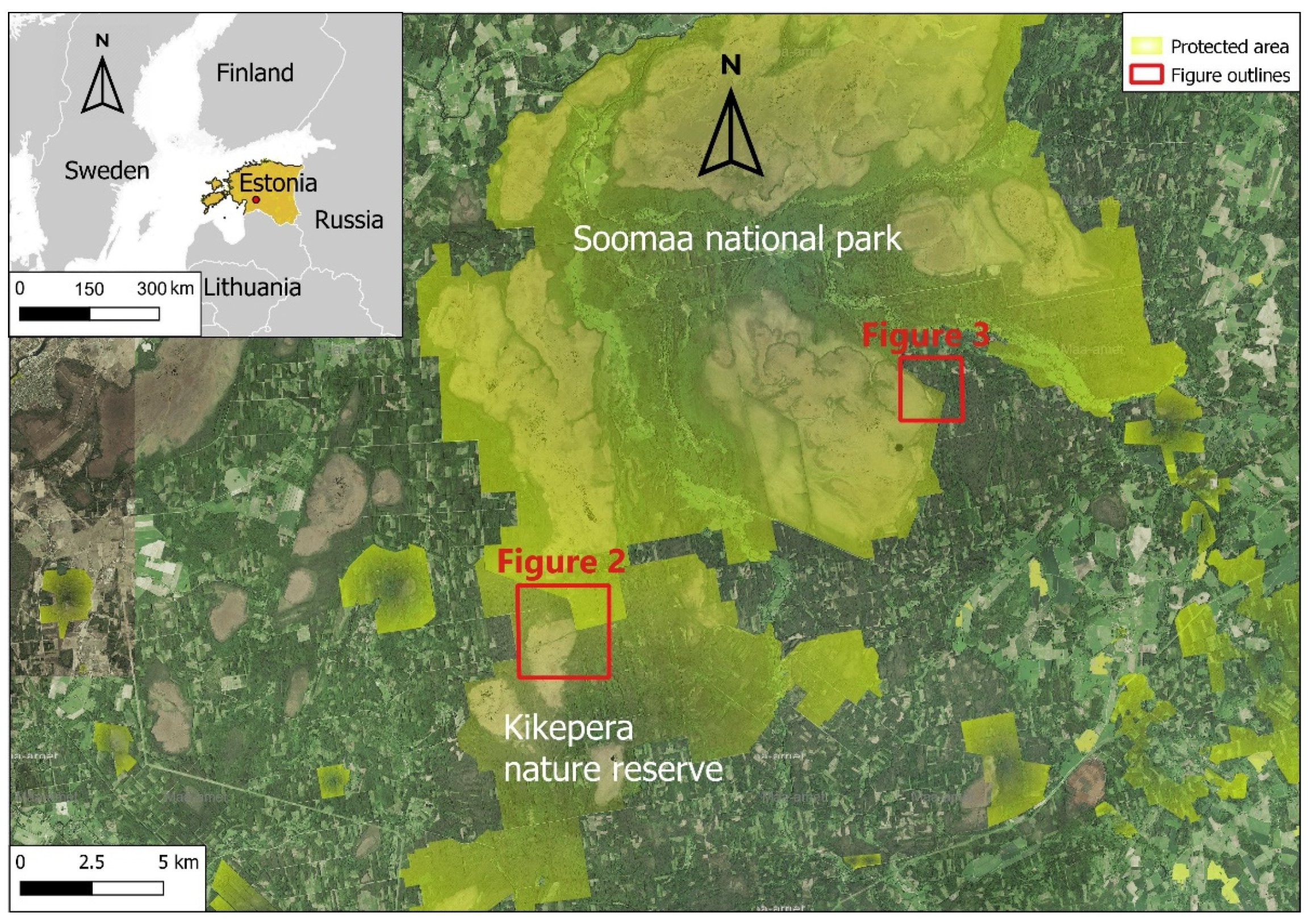
The study area was located in the Soomaa National Park and Kikepera Nature Reserve, in the southwest of Estonia, on the western slope of the Pärnu lowland and the Sakala highland (Figure 1). The area is characterized by numerous mire systems that are divided by rivers and seasonally flooded meadows and forests. We used an ongoing experiment, which was designed in 2013 to restore peatland forest habitats for the Capercaillie (Tetrao urogallus), an iconic bird species in the Baltic States [28]. The experiment combined ditch closure (backfilling where possible; damming elsewhere and in combination) and partial harvest treatments in a block design, and targeted mixotrophic bog areas drained in the late 1960s. These treatments were similar to the ones used in Estonia and elsewhere for more general mire habitat restoration [8,29], but the intensity was adjusted to the specific objective of sustaining forest cover.
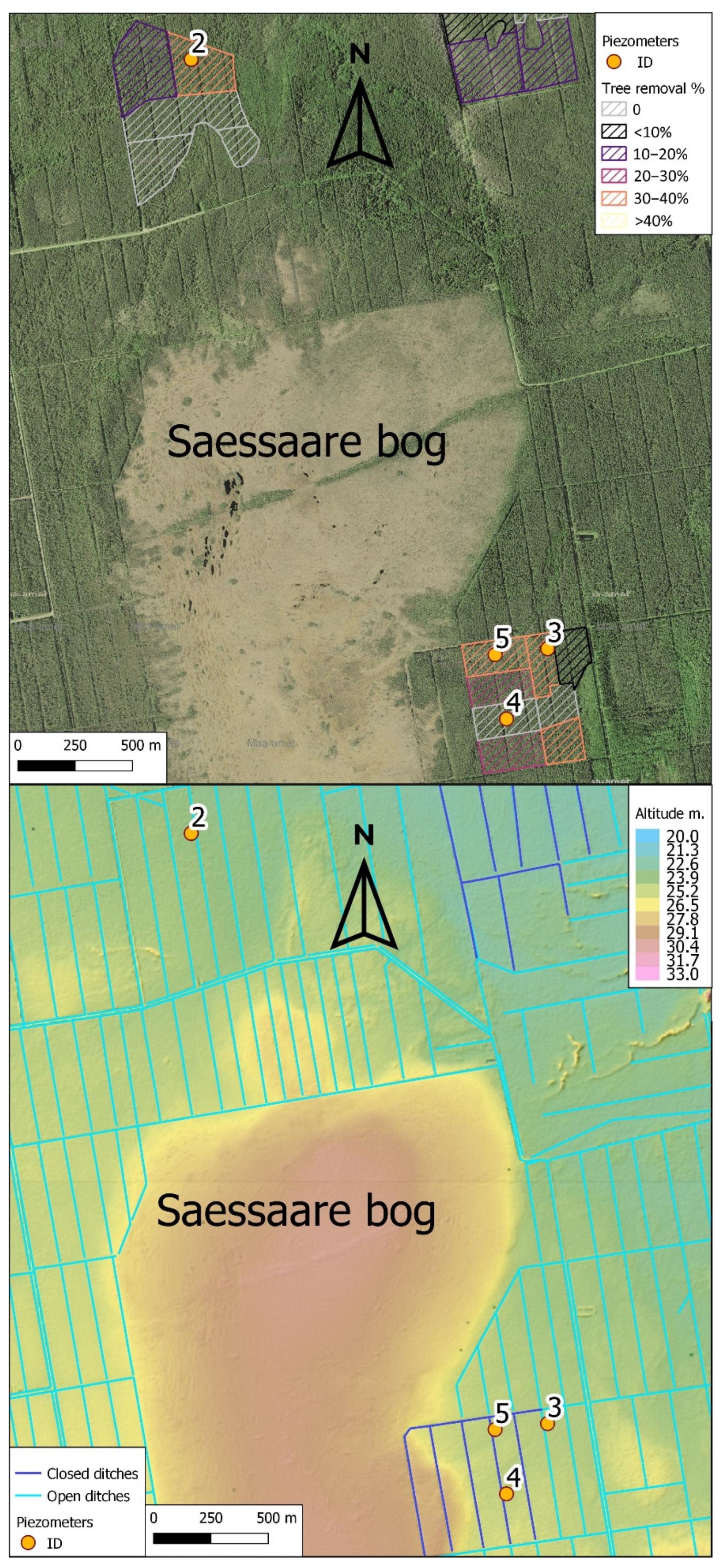
For this study, five plots were selected in order to assess the model simulations against measured groundwater level fluctuations under different manipulations and site conditions (Table 1). As shown in Figure 2 and Figure 3, the drainage ditches in the study area were arranged in rectangular shapes. The plots differed in peat layer thickness, altitude, and forest stand density. The altitude is related to the surface slope required for surface runoff calculations. Since the plots were separated by the drainage ditches, their local treatments were unlikely to have considerable influence on each other. However, the surface water can also reach geographically lower plots over the ditches. In order to include that effect in lower-lying plots, we varied the model values of the amount of precipitation in the period prior to ditch closure. The amount of precipitation was chosen as the input parameter to be adjusted given its linear relationship with the surface runoff [30] that forms water in ditches.
Of other parameters, the peat thickness was measured in the field. Information about the underlying mineral soil (5 m of till in our case) and sedimentary rocks (Devonian sandstones) is based on the geological mapping at the scale of 1:400,000 (Estonian Land Board) and separate peat resource maps (scale 1:10,000, Estonian Geological Survey).
2.2. The Modelling Techniques
A detailed description of the model, including its calculations, parameterization techniques, sub-models and feedbacks, is available in [23]. In the current study, the simulation was applied to the period from 1 November 2013 to 31 December 2018. The temporal resolution for the model was one day; there were altogether 1836 data points (days). The input data set contained: (i) meteorological data of daily means (rain and snow; air temperature; relative humidity; wind speed; solar radiation) as obtained from the state-run weather stations at Kaansoo and Türi; (ii) remote sensing data (reflectance in red and near infrared bounds before and after thinning of the forest stand) sourced from the Estonian Land Board; (iii) geological and geomorphological data (peat layer thickness; slope of the surface of the plot); (iv) soil hydraulic properties (peat layer wetting front suction head; peat and sandstone total porosity and effective porosity; peat residual saturation and peat saturated hydraulic conductivity) [31,32,33,34,35,36], and (v) values calculated (leaf distribution angle; specific leaf storage; snow interception coefficient; maximum snow storage in the tree canopy; peat evaporation coefficient; limestone percolation coefficient).
Of the calculated values, the leaf distribution angle ranged between 0.2 and 0.8; specific leaf storage was between 0.4 and 5.88 [22]. To calculate the snow interception, we modified the rain interception equation [7] and concluded, after the calibration, that the exact value can be searched within the range of 2 to 8. The peat evaporation coefficient is an exponent greater than 1 [21]. For water percolation in sandstone, we developed a new approach where it is calculated on the basis of peat layer’s water deficit (OiP), peat effective porosity (OeP), sandstone field capacity (OfS), effective moisture saturation of peat layer (SmP), and sandstone percolation coefficient (IS):
IF OiP > OeP
THEN (SmP/OfS)*IS
ELSE 0
THEN (SmP/OfS)*IS
ELSE 0
The sandstone percolation coefficient was determined as 0.0019 during the calibration.
To address the experimental treatments (stand thinning and ditch closure), remote sensing data obtained from flights over the area before and after the tree felling was used to calculate the size of the forest stand and the LAI (from reflectance in the red and near red spectrum). We acknowledge that the LAI reduction is not always proportional to partial tree cutting; for example, when shrub layer responds to opening up the canopy with a rapid growth. Ditch closure was simulated by changing the slope of the ground surface that causes runoff reduction.
The simulation model coefficients were calibrated only once using the test plot 1 (Table 1). Those calibrated values were also used in the other plots, the plot-specific input variables being the thickness of the peat layer, reflectance in the red and near infrared bound, and the slope of the surface. The post-thinning reflectance measurements for the test plot were not available and were therefore addressed by fitting appropriate values until the simulated groundwater curve approached as close as possible to the groundwater measurements. This serves as an example of how to apply a calibrated simulation model to find an unknown parameter value.
The model performance was validated by comparing the simulated values of groundwater levels with the measurements performed on site. For the latter, piezometers with a ceramic piezoresistive pressure sensor (push-in type, manufactured by Geotech AB, Askim, Sweden) were used. All piezometers were installed at depth of 1.16 m and positioned 15 m away from the nearest drainage ditch. The piezometers measured the pressure and temperature at 8 h intervals. The air pressure was later subtracted from the total pressure in order to get the water column height above the sensor.
3. Results
3.1. Accuracy of Groundwater Level Simulations
The model performance varied among the test plots (Table 2). The mean difference between simulated and observed groundwater level estimates was 0.88–2.63 cm. The absolute mean differences between the estimates were smaller in those plots where the groundwater levels fluctuated less. In parallel, the root mean square error (RMSE) value was lower in the plots where the difference between the two curves was smaller. In contrast, correlation coefficients and R2 values were closer to 1 (showing closer co-variation) in the plots where more extensive ecosystem restoration work had been performed. In all plots, the Nash-Sutcliffe efficiency coefficients (NSE) were above zero, indicating that the model was not biased and had a potential for forecasting [37].
Below, the model performance in each plot is examined in more detail.
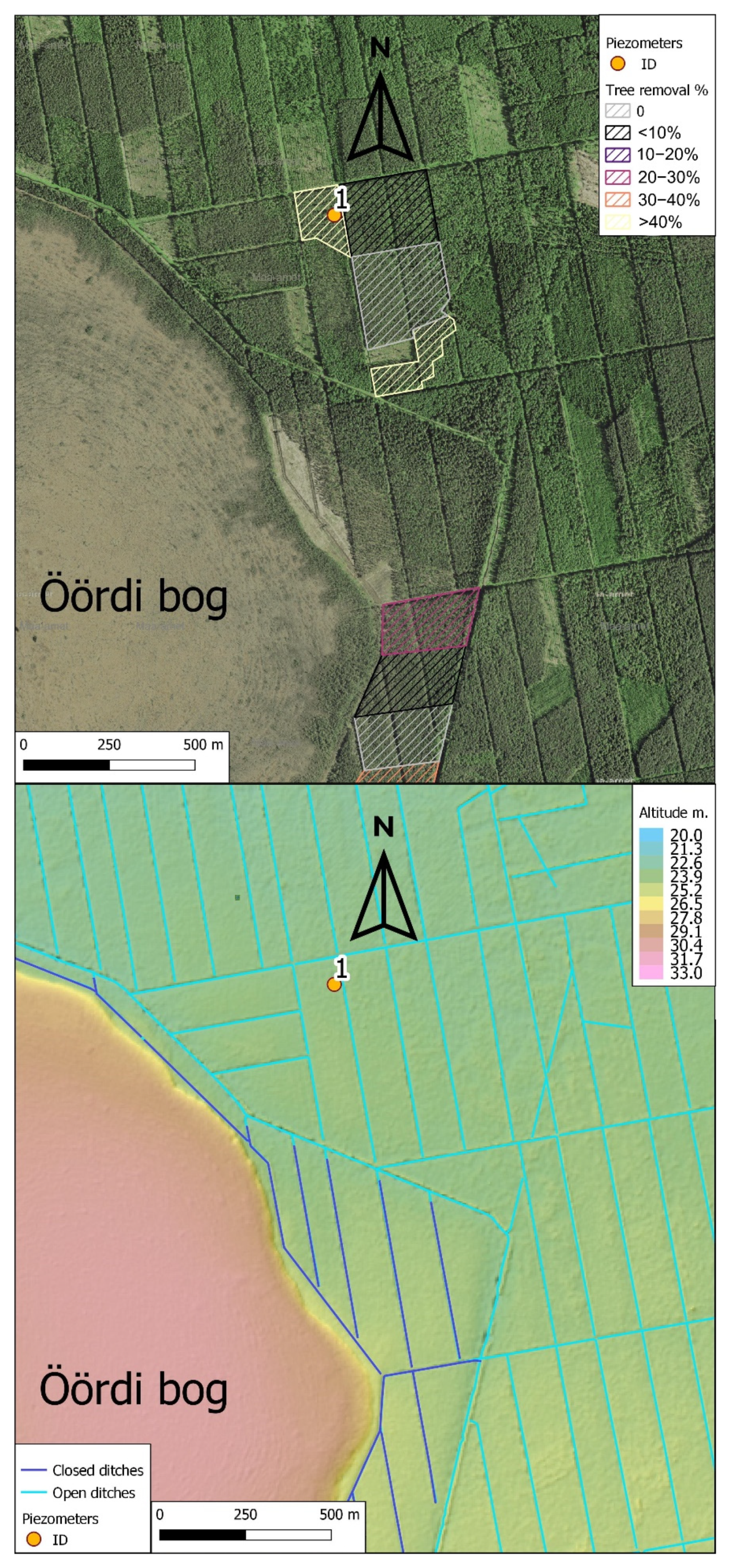
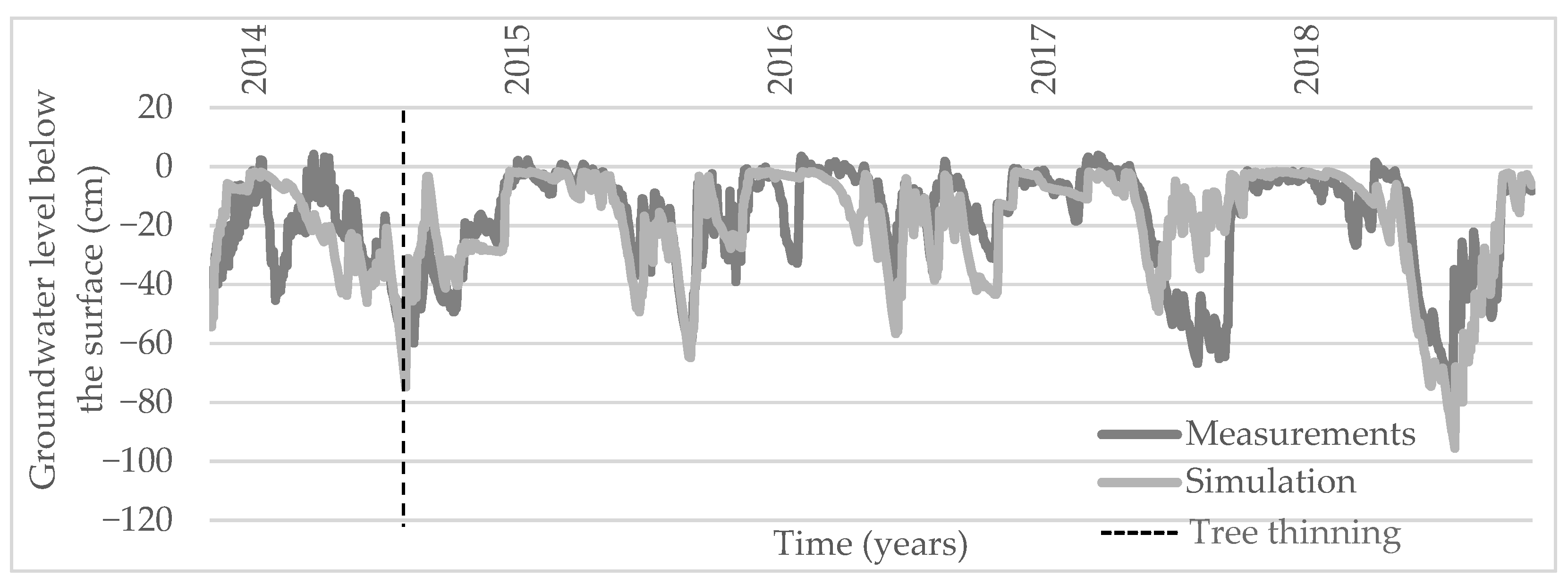
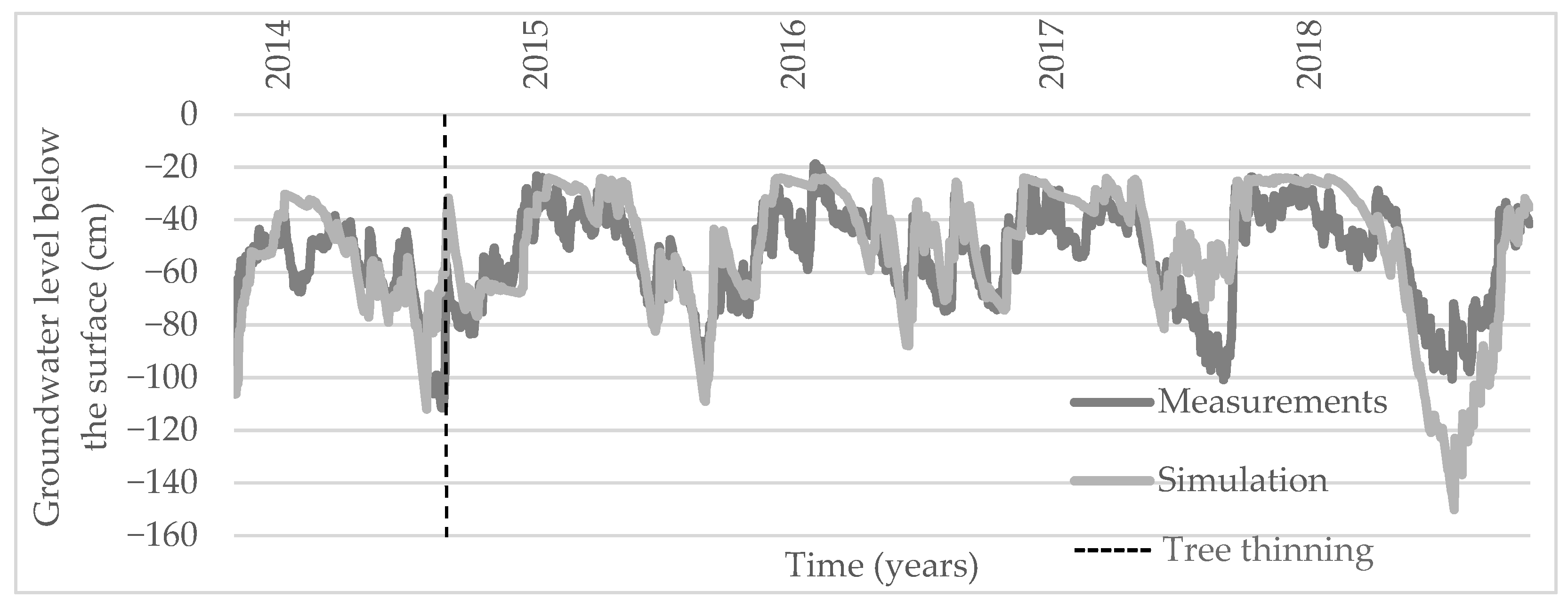
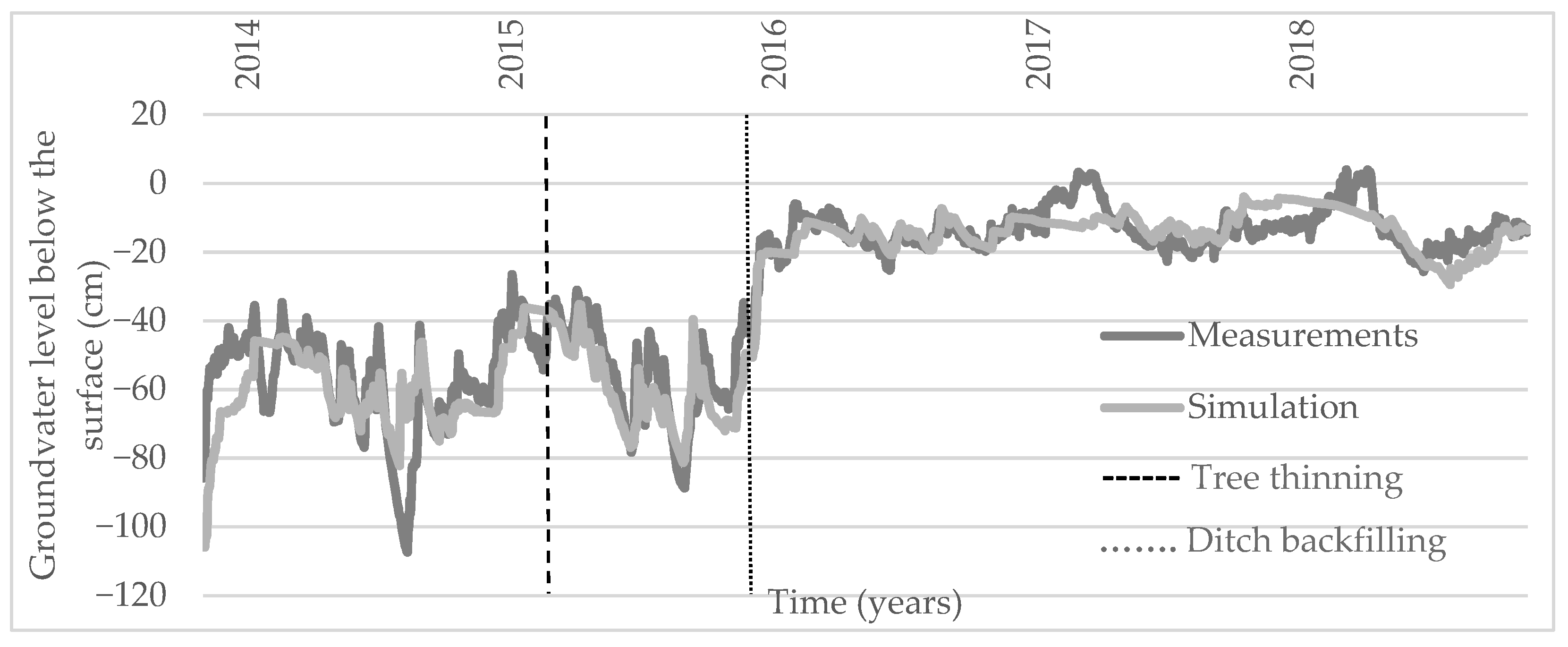
The plot 1 was located at 39 m above the sea level, higher up than the surrounding area (Figure 2). Its groundwater level dynamics indicated a contribution from the thinning of the forest stand (44% removal on 14 August 2014; the vertical line in Figure 4): from 2015, there were no significant fluctuations in winter and the groundwater level remained a few cm below the surface. However, fluctuations re-appeared with the onset of warmer weather and the thawing of the slopes of the drainage ditches; these fluctuations exceeded those typical of a natural raised bog (within +/−30 cm from the ground surface) [38].
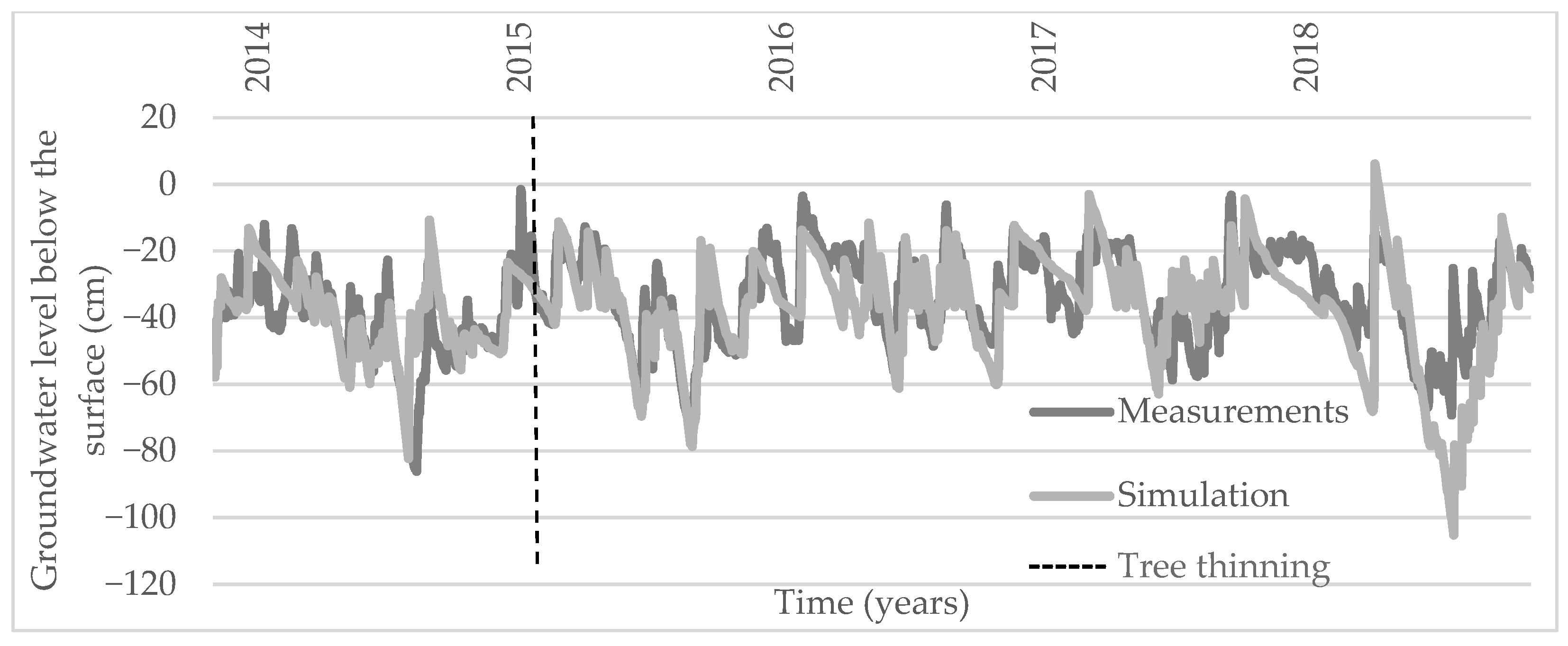
The groundwater curves of the plot 2 (Figure 5) reveal elevated groundwater levels in the post-thinning winter (2014/2015). On frozen ground there is no evaporation, but, unlike deciduous trees, conifers slowly transpire. Nevertheless, the peat layer loses less water. In summer, the impact of the decrease in transpiration on the total water balance was less pronounced. A likely explanation is that the thinning exposed the undergrowth, where the extra atmospheric heat and solar radiation caused an increase in evaporation.
Three plots (3, 4 and 5) were located close to each other (see Figure 2) but were separated and bound by a system of drainage ditches. The thinned plot 3 was located above the other two plots. Its measured and simulated groundwater level curves matched most closely among all the plots (Figure 6; Table 3) supporting the view that simulated curves can become very close to the measured ones.
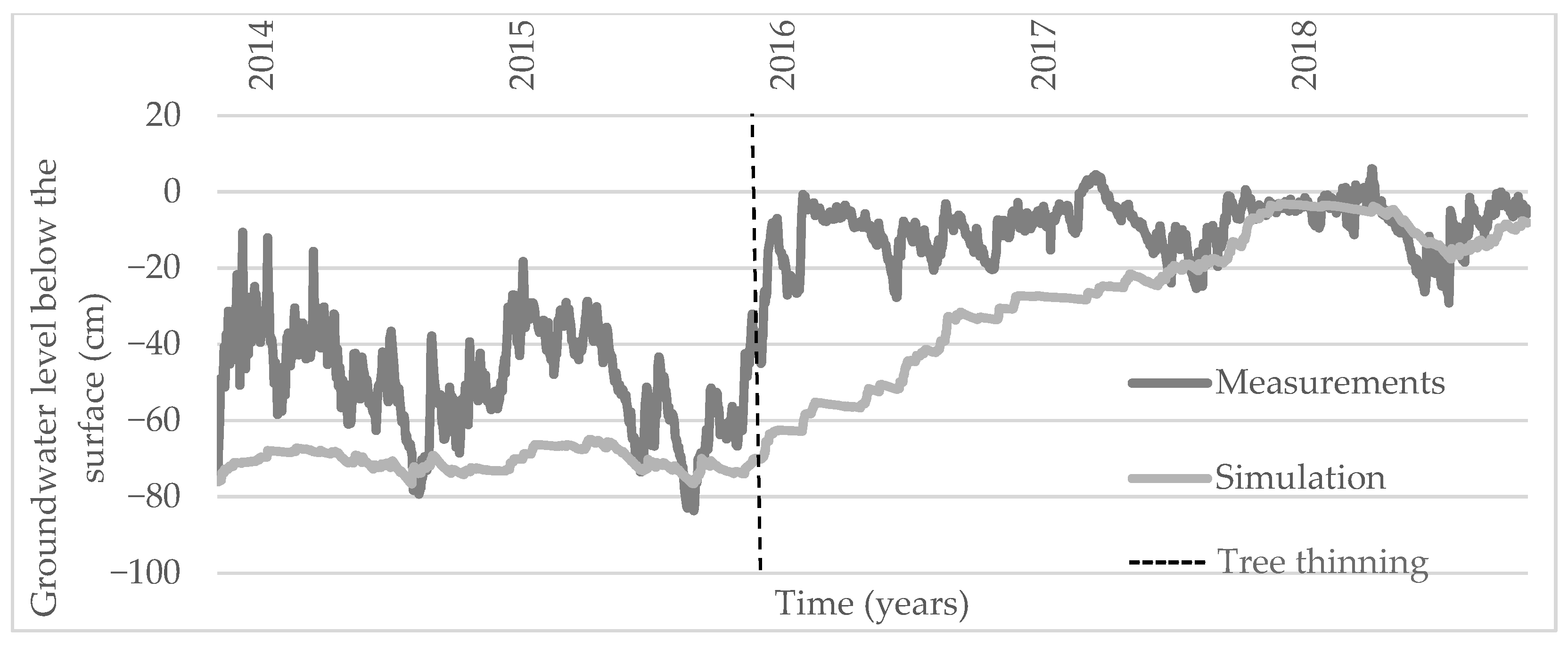
The unthinned plot 4 was located at 31 m above the sea level and one metre below the plot 3 (Figure 2); it only received the ditch closure treatment (backfilling with peat). Figure 7 shows that the simulated estimates of its groundwater level started significantly below the actual levels. Following the closure of the drainage ditches in December 2015, the simulated values gradually increased until, in summer 2017, they reached the measured groundwater levels and followed those further.
Such a behaviour of the simulated curve has a technical explanation: it was not possible to simulate a steeper increase in the groundwater level following the closure of the ditches when using precipitation as the only source of water supply (see also Section 2.1). Infiltration in the peat layer should exceed the amount of precipitation several times in order to reach the measured groundwater levels. Thus, after backfilling of the ditches, the plot 4 was modelled as receiving only the actual amount of precipitation, since the impact of adjacent sections was significantly reduced. Yet some surface runoff from adjacent plots may have actually reached it over the surface.
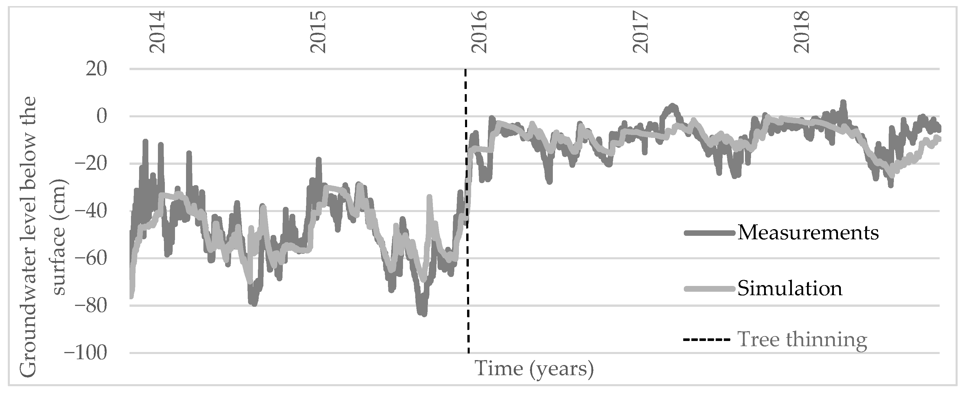
A support that plots 4 and 5 were affected from geographically higher areas even after the backfilling of the ditches was found in spring 2017 when a thick snow cover was formed. During this period, the measured groundwater levels were apparently enriched with a larger mass of water than produced by the snow precipitation alone (Figure 8). The amount of water to accurately simulate the observed fluctuations in the groundwater level in the plot 4 was achieved by increasing the precipitation parameter values 5.2 times.
The plot 5 received a distinct combined treatment of ditch backfilling with peat soil and 34% tree removal (the vertical lines in Figure 9). It was lower-lying than the other plots (30 m above sea level) and all the drainage ditches separating it from the raised bog in the west were closed during the experiment (Figure 3). Being located approximately one meter below the plot 4, the drainage impact on its water balance was even more pronounced here. In order to fit the simulated groundwater level curve with the observations, the precipitation parameter should be increased 6.2 times for the period before the ditch closure, but only 1.7 times after the backfilling. This difference probably reflects the share of the surface runoff from higher areas.
3.2. Performance of the Leaf Area Index as Vegetation Proxy
The LAI was not directly proportional to the extent of tree removals at thinning (Table 3). This can be explained by the compensatory responses of the undergrowth after opening up of the canopies (see above).
4. Discussion
Our simulation model validation, in terms of the turning points in the time series, indicated that its mathematical equations work correctly. However, the mean differences between the observed and simulated groundwater curves were smaller in the case of smaller groundwater level fluctuations. A general implication is that such models more accurately simulate the absolute impacts of smaller interventions to the ecosystem. This contrasts with a practical necessity for such models, specifically in the case of large (planned) interventions, which risk potentially large unwanted environmental impacts and inefficient expenditure of funds. To address this problem, a relative assessment of the performance of the model was provided by the correlation coefficients and R2 values. These estimates of the system dynamics were indeed better in the plots with more intensive restoration treatments. Ecologically, such strong correlations indicate that the simulation model successfully detected the rapid increase in the saturation of the peat layer after drainage ditches were back-filled.
An advantage of our model is that it can be operated in any System Dynamics (SD) environment. It is tested and works equally well in using both Stella Architect version 1.9.4, ISEE systems Inc., Lebanon, PA, USA and Insight Maker software. Its main problems are thus related to the general spatial limitations of the SD modelling framework. Specifically, in lower lying plots, which received water not only from precipitation but also from the adjacent areas (as surface runoff), our simulation equations did not work accurately without resolving for additional water supplies. This problem could be solved by transferring the tested equations to another simulation modelling environment. A promising modelling environment would allow the whole catchment area to be defined based on a GIS digital terrain model [39]; then, either agent-based modelling [40,41] could be used, or a new modelling tool in the Python programming language [42,43] developed. In agent-based models, ‘agents’ are the components capable of moving and responding to the local environment. In our case, the agents would track a water path that goes through a catchment at a given moment; similarly to the patterns in system dynamics, they could make ‘decisions’ on the paths. Python is a very popular programming language for scientific computing due to a low barrier to entry for translating ideas into code and generating actual data [44].
Expanding the geographic area would allow our simulation model to be applied to real bog restoration projects, while an agent-based modelling approach could open up possibilities for even wider uses. For example, replacing the peat parameters with those of mineral soils (supplemented with a couple of other corrections) could open a way to use the model in precise agriculture. The practical problems addressed could then include the absorption of fertilizers through roots and degradation in soil, depending on the seeded plant species, thereby providing insights into an optimal use of fertilisers.
A general message from our study is that the SD approach appears a promising first step for process-based models. It can simulate hydrological processes at specific locations, helping to understand the causes, consequences and a sufficient set of system components, before simulating large-scale processes in an advanced environment.
Author Contributions
O.J. proposed the idea of the main text, constructed the manuscript, developed a new percolation in sandstone approach, conducted model verification, and contributed to the tables and figures. M.K. provided hydrological and meteorological data, contributed to the main text, and figures. A.L. developed the experimental systems, provided vegetation data, and contributed to the main text and structure of the manuscript. All authors have read and agreed to the published version of the manuscript.
Funding
Funding was provided by the University of Tartu Dora Plus sub-activity 2.2 grant for international visiting doctoral students (to O.J.) and the Estonian Research Council (project IUT 34-7 and PRG1121 to A.L.).
Institutional Review Board Statement
Not applicable.
Informed Consent Statement
Not applicable.
Data Availability Statement
The data presented in this study are available on request from the corresponding author.
Acknowledgments
We are grateful to the Estonian State Forest Management Centre for carrying out the habitat manipulations.
Conflicts of Interest
The authors declare no conflict of interest.
References
- Hepburn, C.; O’Callaghan, B.; Stern, N.; Stiglitz, J.; Zenghelis, D. Will COVID-19 fiscal recovery packages accelerate or retard progress on climate change? Oxf. Rev. Econ. Policy 2020, 36, S359–S381. [Google Scholar] [CrossRef]
- Kiely, G.; Leahy, P.; Mcveigh, P.; Lewis, C.; Sottocornola, M.; Laine, A.; Koehler, A.-K. PeatGHG-Survey of GHG Emission and Sink Potential of Blanket Peatlands; Environmental Protection Agency: Wexford, Ireland, 2018.
- Kimmel, K.; Mander, Ü. Ecosystem services of peatlands: Implications for restoration. Prog. Phys. Geogr. 2010, 34, 491–514. [Google Scholar] [CrossRef]
- Andersen, R.; Farrell, C.; Graf, M.; Muller, F.; Calvar, E.; Frankard, P.; Caporn, S.; Anderson, P. An overview of the progress and challenges of peatland restoration in Western Europe. Restor. Ecol. 2017, 25, 271–282. [Google Scholar] [CrossRef]
- Mitsch, W.J.; Straškraba, M.; Jørgensen, S.N. Wetland Modelling. Developments in Environmental Modelling; Elsvier: Amsterdam, The Netherlands, 1988; ISBN 9780444597694. [Google Scholar]
- Lamers, L.P.; Vile, M.A.; Grootjans, A.P.; Acreman, M.C.; van Diggelen, R.; Evans, M.G.; Richardson, C.J.; Rochefort, L.; Kooijman, A.M.; Roelofs, J.G.; et al. Ecological restoration of rich fens in Europe and North America: From trial and error to an evidence-based approach. Biol. Rev. 2015, 90, 182–203. [Google Scholar] [CrossRef] [Green Version]
- Java, O. Significance of thinning degraded swamps forest stand in sustainable ecosystem’s development. In Proceedings of the 8th International Scientific Conference Rural Development 2017, Kaunas, Lithuania, 23–24 November 2017; pp. 1–5. [Google Scholar]
- Anderson, R.; Vasander, H.; Geddes, N.; Laine, A.; Tolvanen, A.; O’Sullivan, A.; Aapala, K. Afforested and forestry-drained peatland restoration. In Peatland Restoration and Ecosystem Services—Science, Policy and Practices; Bonn, A., Allott, T., Evans, M., Joosten, H., Stoneman, R., Eds.; Cambridge University Press: Cambridge, UK, 2016; pp. 213–233. [Google Scholar]
- Remm, L.; Lõhmus, A.; Leibak, E.; Kohv, M.; Salm, J.O.; Lõhmus, P.; Rosenvald, R.; Runnel, K.; Vellak, K.; Rannap, R. Restoration dilemmas between future ecosystem and current species values: The concept and a practical approach in Estonian mires. J. Environ. Manag. 2019, 250, 1–8. [Google Scholar] [CrossRef]
- Chen, B.; Liu, Z.; He, C.; Peng, H.; Xia, P.; Nie, Y. The regional hydro-ecological simulation system for 30 years: A systematic review. Water 2020, 12, 2878. [Google Scholar] [CrossRef]
- Koohestani, N.; Meftah Halaghi, M.; Dehghani, A. Numerical simulation of groundwater level using MODFLOW software (A case study: Narmab watershed, Golestan province). Int. J. Adv. Biol. Biomed. Res. 2013, 1, 858–873. [Google Scholar]
- Longcang, S.; Yang, X.; Peieng, W. Groundwater Flow Numeric Simulation Method Based on Uncertaintiesof MODFLOW Parameters. J. Jilin Univ. Earth Sci. Ed. 2017, 47, 1803–1809. [Google Scholar] [CrossRef]
- Akter, A.; Ahmed, S. Modeling of groundwater level changes in an urban area. Sustain. Water Resour. Manag. 2021, 7, 1–20. [Google Scholar] [CrossRef]
- Texas A&M University. Soil & Water Assessment Tool. Available online: https://swat.tamu.edu/ (accessed on 18 June 2021).
- O’Keeffe, J.; Marcinkowski, P.; Utratna, M.; Piniewski, M.; Kardel, I.; Kundzewicz, Z.W.; Okruszko, T. Modelling climate change’s impact on the hydrology of Natura 2000 wetland habitats in the Vistula and Odra River Basins in Poland. Water 2019, 11, 2191. [Google Scholar] [CrossRef] [Green Version]
- Stockholm Environment Institute Why WEAP? Available online: https://www.weap21.org/index.asp?action=201 (accessed on 18 June 2021).
- DHI MIKE SHE. Available online: https://www.mikepoweredbydhi.com/products/mike-she (accessed on 18 June 2021).
- Natural Resources Conservation Service HEC-RAS. Available online: https://go.usa.gov/xXcRM (accessed on 18 June 2021).
- Tufts University Modeling Framework for Simulating, River, Stream, and Lake Water Quality. Available online: http://www.qual2k.com/home/default.html (accessed on 18 June 2021).
- Forrester, J.W. System dynamics, systems thinking, and soft OR. Syst. Dyn. Rev. 1994, 10, 245–256. [Google Scholar] [CrossRef]
- Elshorbagy, A.; Jutla, A.; Barbour, L.; Kells, J. System dynamics approach to assess the sustainability of reclamation of disturbed watersheds. Can. J. Civ. Eng. 2005, 32, 144–158. [Google Scholar] [CrossRef]
- Keshta, N.; Elshorbagy, A.; Carey, S. A generic system dynamics model for simulating and evaluating the hydrological performance of reconstructed watersheds. Hydrol. Earth Syst. Sci. 2009, 13, 865–881. [Google Scholar] [CrossRef] [Green Version]
- Java, O. Restoration of a degraded bog hydrological regime using System Dynamics modeling. CBU Int. Conf. Proc. 2018, 6, 1105–1113. [Google Scholar] [CrossRef] [Green Version]
- Java, O.; Kohv, M.; Lõhmus, A. Hydrological model for decision-making: Männikjärve bog case study, Estonia. Balt. J. Mod. Comput. 2020, 8, 379–390. [Google Scholar] [CrossRef]
- Gong, P.; Pu, R.; Biging, G.S.; Larrieu, M.R. Estimation of forest leaf area index using vegetation indices derived from Hyperion hyperspectral data. IEEE Trans. Geosci. Remote Sens. 2003, 41, 1355–1362. [Google Scholar] [CrossRef] [Green Version]
- Zheng, G.; Moskal, L.M. Retrieving Leaf Area Index (LAI) Using Remote Sensing: Theories, Methods and Sensors. Sensors 2009, 9, 2719–2745. [Google Scholar] [CrossRef] [Green Version]
- Yu, Y.; Wang, J.; Liu, G.; Cheng, F. Forest Leaf Area Index inversion based on Landsat OLI data in the Shangri-La City. J. Indian Soc. Remote. Sens. 2019, 47, 967–976. [Google Scholar] [CrossRef]
- Lõhmus, A.; Leivits, M.; Pēterhofs, E.; Zizas, R.; Hofmanis, H.; Ojaste, I.; Kurlavičius, P. The Capercaillie (Tetrao urogallus): An iconic focal species for knowledge-based integrative management and conservation of Baltic forests. Biodivers. Conserv. 2017, 26, 1–21. [Google Scholar] [CrossRef]
- Laine, A.M.; Leppälä, M.; Tarvainen, O.; Päätalo, M.L.; Seppänen, R.; Tolvanen, A. Restoration of managed pine fens: Effect on hydrology and vegetation. Appl. Veg. Sci. 2011, 14, 340–349. [Google Scholar] [CrossRef]
- Abudu Kasei, R.; Ampadu, B.; Sapanbil, G.S. Relationship between rainfall-runoff on the White Volta River at Pwalugu of the Volta Basin in Ghana. J. Environ. Earth Sci. 2013, 3, 92–100. [Google Scholar]
- Custers, J.; Graafstal, H. Characterisation of the Water Flow in a Pool-Ridge Microtope in a Bog. A Case Study of Männikjärve Bog, Estonia; Unpublished Report; Wageningen University: Wageningen, The Netherlands; Tallinn University: Tallinn, Estonia, 2005. [Google Scholar]
- Liu, H.; Lennartz, B. Hydraulic properties of peat soils along a bulk density gradient—A meta study. Hydrol. Process. 2019, 33, 101–114. [Google Scholar] [CrossRef] [Green Version]
- Rawls, W.J.; Brakensiek, D.L.; Saxton, K.E. Estimation of soil water properties. Trans. ASAE 1982, 25, 1316–1320. [Google Scholar] [CrossRef]
- da Silva, F.F.; Wallach, R.; Chen, Y. Hydraulic properties of sphagnum peat moss and tuff (scoria) and their potential effects on water availability. Plant Soil 1993, 154, 119–126. [Google Scholar] [CrossRef]
- Fuel, S.N.; Kellner, E. Svensk Kärnbränslehantering AB Effects of Variations in Hydraulic Conductivity and Flow Conditions on Groundwater Flow and Solute Transport in Peatlands. C. Grup. AB; Technical Report; Swedish Nuclear Fuel and Waste Management Co.: Stockholm, Sweden, 15 February 2007; pp. 1–55. [Google Scholar]
- Schlotzhauer, S.M.; Price, J.S. Soil water flow dynamics in a managed cutover peat field, Quebec: Field and laboratory investigations. Water Resour. Res. 1999, 35, 3675–3683. [Google Scholar] [CrossRef]
- Moussa, R. When monstrosity can be beautiful while normality can be ugly: Assessing the performance of event-based flood models. Hydrol. Sci. J. 2010, 55, 1074–1084. [Google Scholar] [CrossRef]
- Krīgere, I.; Kalniņa, L.; Dreimanis, I.; Lazdiņš, A.; Pakalne, M. Rewetting (re-creating mire conditions). In Sustainable and Responsible After-Use of Peat Extraction Areas; Priede, A., Gancone, A., Eds.; Biedrība “Baltijas krasti”: Riga, Latvia, 2019; pp. 195–201. ISBN 9789934198458. [Google Scholar]
- Miller, S.N.; Semmens, D.J.; Miller, R.C.; Hernandez, M.; Goodrich, D.C.; Miller, W.P.; Kepner, W.G.; Ebert, D. GIS-Based Hydrologic Modeling: The Automated Geospatial Watershed Assessment Tool. In Proceedings of the 2nd Federal Interagency Hydrologic Modleing Conference, Las Vegas, NV, USA, 28 July–1 August 2002; pp. 1–12. [Google Scholar]
- Reaney, S.M. The use of agent based modelling techniques in hydrology: Determining the spatial and temporal origin of channel flow in semi-arid catchments. Earth Surf. Process. Landf. 2008, 33, 317–327. [Google Scholar] [CrossRef]
- Huber, L.; Bahro, N.; Leitinger, G.; Tappeiner, U.; Strasser, U. Agent-based modelling of a coupled water demand and supply system at the catchment scale. Sustainability 2019, 11, 6178. [Google Scholar] [CrossRef] [Green Version]
- Collenteur, P.; Mälicke, M.; Visser, M.; Vremec, M. Python-Hydrology-Tools. Available online: https://github.com/raoulcollenteur/Python-Hydrology-Tools (accessed on 8 August 2021).
- Python Software Foundation Applications for Python. Available online: https://www.python.org/about/apps/ (accessed on 30 June 2021).
- Comparing Python and Julia for Hydrological Modeling. Available online: https://medium.com/@kel.markert/comparing-python-and-julia-for-hydrologic-modeling-7334ffa9534b (accessed on 2 August 2021).
Figure 1.
Location of the study area and test plots.

Figure 2.
Ortophoto, digital terrain model, locations of the forest manipulations, and piezometers in the southern part of the study area, Kikepera Nature Reserve (data from the Estonian Land Board).
Figure 2.
Ortophoto, digital terrain model, locations of the forest manipulations, and piezometers in the southern part of the study area, Kikepera Nature Reserve (data from the Estonian Land Board).

Figure 3.
Ortophoto, digital terrain model, locations of the forest manipulations, and piezometers in the northern part of the study area study area (data from the Estonian Land Board).
Figure 3.
Ortophoto, digital terrain model, locations of the forest manipulations, and piezometers in the northern part of the study area study area (data from the Estonian Land Board).

Figure 4.
Measured vs. simulated groundwater level in plot 1.

Figure 5.
Measured vs. simulated groundwater level in plot 2.

Figure 6.
Measured vs. simulated groundwater level in plot 3.

Figure 7.
Measured vs. simulated groundwater level in plot 4.

Figure 8.
Groundwater level estimates for plot 4 after adjusting the precipitation parameter to include the water supply from surface runoff.
Figure 8.
Groundwater level estimates for plot 4 after adjusting the precipitation parameter to include the water supply from surface runoff.

Figure 9.
Plot 5 groundwater level after manipulation with the amount of precipitation.


Table 1.
Characteristics of the study plots.
| ID | Peat (m) | Date of Forest Thinning | Date of Closure of Drainage Ditches | Tree Removal at Thinning (%) |
|---|---|---|---|---|
| 1 | 0.8 | 14.08.2014 | Not performed | 44 |
| 2 | 1.2 | 15.10.2014 | Not performed | 31 |
| 3 | 1.2 | 15.02.2015 | Not performed | 38 |
| 4 | 1.3 | Not performed | 01.12.2015 | 0 |
| 5 | 1.2 | 18.02.2015 | 01.12.2015 | 34 |
Table 2.
Parameters that indicate the accuracy of the simulation model by study plots.
| ID | Mean Difference (cm) | Correlation | R2 | RMSE | NSE |
|---|---|---|---|---|---|
| 1 | 0.96 | 0.70 | 0.50 | 0.32 | 0.39 |
| 2 | 1.25 | 0.78 | 0.60 | 0.37 | 0.23 |
| 3 | 0.88 | 0.68 | 0.47 | 0.28 | 0.25 |
| 4 | 1.64 | 0.94 | 0.89 | 0.42 | 0.89 |
| 5 | 2.63 | 0.94 | 0.88 | 0.71 | 0.19 |
Table 3.
Characteristics of the forest stands in the study plots.
| ID | NIR before Forest Stand Thinning | Red before Forest Stand Thinning | LAI before Forest Stand Thinning | NIR after Forest Stand Thinning | Red after Forest Stand Thinning | LAI after Forest Stand Thinning | Forest Stand Thinning Intensity (%) | Changes in LAI (%) |
|---|---|---|---|---|---|---|---|---|
| 1 | 85 | 29 | 2.36 | 97 | 53 | 1.76 | 44 | −25 |
| 2 | 77 | 41 | 1.76 | 97 | 60 | 1.54 | 31 | −13 |
| 3 | 52 | 30 | 1.65 | 56 | 41 | 1.28 | 38 | −22 |
| 4 | 59 | 31 | 1.78 | 70 | 36 | 1.81 | 0 | +2 |
| 5 | 37 | 21 | 1.67 | 44 | 26 | 1.61 | 34 | −4 |
Publisher’s Note: MDPI stays neutral with regard to jurisdictional claims in published maps and institutional affiliations. |
© 2021 by the authors. Licensee MDPI, Basel, Switzerland. This article is an open access article distributed under the terms and conditions of the Creative Commons Attribution (CC BY) license (https://creativecommons.org/licenses/by/4.0/).
Share and Cite
MDPI and ACS Style
Java, O.; Kohv, M.; Lõhmus, A. Performance of a Bog Hydrological System Dynamics Simulation Model in an Ecological Restoration Context: Soomaa Case Study, Estonia. Water 2021, 13, 2217. https://doi.org/10.3390/w13162217
AMA Style
Java O, Kohv M, Lõhmus A. Performance of a Bog Hydrological System Dynamics Simulation Model in an Ecological Restoration Context: Soomaa Case Study, Estonia. Water. 2021; 13(16):2217. https://doi.org/10.3390/w13162217
Chicago/Turabian StyleJava, Oskars, Marko Kohv, and Asko Lõhmus. 2021. "Performance of a Bog Hydrological System Dynamics Simulation Model in an Ecological Restoration Context: Soomaa Case Study, Estonia" Water 13, no. 16: 2217. https://doi.org/10.3390/w13162217
Note that from the first issue of 2016, this journal uses article numbers instead of page numbers. See further details here.