Modeling Groundwater-Fed Irrigation and Its Impact on Streamflow and Groundwater Depth in an Agricultural Area of Huaihe River Basin, China

Abstract

The amount of water taken from groundwater for agricultural irrigation is often not observed, while hydrological models have been extensively proposed to investigate the irrigation dynamics and impacts in agricultural areas. In this work, we propose an agro-hydrological model that integrates agricultural irrigation with the traditional Xin’anjiang (XAJ) hydrological model. In particular, the proposed model incorporates the FAO guidelines on crop evapotranspiration into hydrological routing of water balance and flow fluxes in unsaturated and saturated zones. The model was used to calibrate the groundwater irrigation amounts in terms of both the observed river discharge and the groundwater depth in the Xuanwu plain area of the Huaihe River Basin in China. The calibration and sensitivity analyses were performed by the shuffled complex evolution (SCE-UA) method. This method can be applied to a single-objective optimization of model parameters, based on either the river discharge or the groundwater depth, or to a multi-objective optimization of model parameters based on both of these objectives. The results show that the multi-objective calibration is more efficient than the single-objective method for capturing dynamics of the river discharge and the groundwater depth. The estimated means of the annual groundwater withdrawal for wheat and maize irrigations were found to be about 140.5 mm and 13.7 mm, respectively. The correlation between the groundwater withdrawal and the change in groundwater depth during crop growing seasons demonstrated that the groundwater withdrawal is the dominant factor for the groundwater depth change in the river basin, particularly in the winter wheat season. Moreover, model simulations show that the combined effects of the reduced precipitation and the increased groundwater withdrawal would lead to a decrease of the average annual runoff and an increase of the average groundwater depth. These estimates can greatly help in understanding the irregular changes in the groundwater withdrawal and offer a quantitative basis for studying future groundwater demands in this area.

1. Introduction

Agricultural needs account for about 70% of worldwide freshwater withdrawals, while irrigation water accounts for about 90% of all agricultural water usage [1]. Therefore, irrigated agriculture is the main component of water demand and a driver of widespread scarcity of freshwater. Globally, the annual water consumption in irrigation comes mainly from groundwater with a percentage of about 43% (or a volume of 545 km³ yr⁻¹). Moreover, the current irrigated area worldwide is approximately 301 million hectares (ha), of which 38% employs groundwater irrigation. In particular, in terms of the total groundwater-irrigated area, China comes second (with 19 million ha), just after India (with 39 million ha) and before the USA (with 17 million ha). Because of the increased use of groundwater in irrigation, groundwater withdrawal rates could exceed the aquifer recharge rates. It might sooner or later result in the depletion of groundwater resources [2].

Various direct and indirect methods have been developed for estimating groundwater withdrawals from aquifers. The direct methods obtain groundwater abstraction amount from in situ measurements including meter readings at pumping wells and electric power consumption readings given relationship between the power consumption and groundwater abstraction amount in some specific areas. However, data collection by direct methods is time-consuming and laborious due to numerous pumping wells in agricultural areas. Moreover, most measurement facilities give annual statistical averages without reporting detailed measurement variations within each year. Alternatively, indirect methods have emerged in order to estimate groundwater withdrawal in the absence of direct measurement data. For instance, groundwater withdrawal can be estimated based on the water-table fluctuations. This method provides an estimate of groundwater withdrawal according to variations of groundwater depth fluctuations and specific yield in the pumping period [3]. In cultivation areas, the groundwater irrigation amount can be estimated according to the consumptive water use of crops, which comes from both evaporation (E) and crop transpiration (T) under rainy conditions. The evapotranspiration can be estimated by the commonly-used FAO-56 dual approach for irrigation management at the regional scale [4]. In recent decades, remote-sensing techniques have been applied to estimate crop transpiration and soil moisture (e.g., Cruz-Blanco et al. [5]). These efforts can roughly estimate historical groundwater withdrawal for irrigation, but they need verifications of the groundwater withdrawal in relation to the consumptive water use of crops. Such relationship can be developed based on water balance analysis in cultivated areas.

Hydrological models are efficient for evaluating water balance in saturated and unsaturated zones and estimating hydrological components, such as evapotranspiration and groundwater level variations under different climate conditions and the influence of irrigation. The global-scale hydrological models, such as WaterGAP [6], PCR-GLOBWB [7], WBMplus [8], GEPIC [9], and LPJmL [10], have been successfully used to estimate the worldwide irrigation amount. Some catchment-scale hydrological models, including the SWAP model [11] and the SWAT model [12], have been improved to augment functions that can quantify irrigation schemes.

One of key procedures for hydrological modelling is parameter calibration and model validation based on available observation data. In order to reduce uncertainties of the modeling results, more observation data are necessary, such as combination uses of discharge and groundwater depth observations in cultivated areas. Meanwhile, an appropriate optimal method can reduce uncertainty of the optimized parameters. Traditional parameter calibration methods based on optimizing a single objective usually fail to reflect the multiple hydrological processes [13] and thus could result in equifinality of the calibrated parameters. In recent decades, many global optimization algorithms have been proposed for parameter calibration. The commonly used algorithms include Genetic Algorithm [14], Particle Swarm Optimization [15], Bayesian Method [16], etc. These multi-objective optimization approaches can effectively reduce the modelling uncertainty [17,18]. The aforementioned approaches are mostly applied to calibrate hydrological parameters and evaluate the effectiveness of hydrological simulations of the rainfall–runoff response and groundwater table dynamics. Nevertheless, these approaches are seldom used to evaluate water use in irrigated agriculture.

The main objectives of this work are to estimate the groundwater use in irrigation and evaluate the reliability of water use simulations. The execution is based on the improved Xin’anjiang (XAJ) hydrological model [19] with functions for estimating the actual FAO crop evapotranspiration and evaluating the groundwater balance induced by the groundwater withdrawal, precipitation recharge and stream flow discharge. The improve model is applied in the Xuanwu catchment of the Huaihe River Basin in China. The single-objective and multi-objective optimization approaches are constructed for model parameter calibration and validation against the catchment outlet discharge and the groundwater depth.

2. Study Area and Data

The Huaihe River Basin is the third most populated river basin and the main agricultural production base in China with about 133,300 km² of cultivated land area, which produces about 1/6 of the total grain output in China. Since the 1960s, the cultivated scheme in this basin has shifted from three harvests every two years to two harvests every single year, one for winter wheat and another for summer maize. As a result, grain production requirements of this wheat-maize cropping system have remarkably increased water demands. The mean annual precipitation is 738 mm, while the average water requirement for the wheat-maize cropping system is generally 700 mm. Because of extremely uneven distribution of intra-annual precipitation, precipitation in the area is not sufficient to meet crop water requirements. Currently, the sustainability of high-level productivity is heavily dependent on the availability of irrigation resources. Groundwater has been exploited to compensate for surface water deficits and hence meet agricultural water requirements. However, the long-term over-exploitation of groundwater has led to significant decline of groundwater table in some areas. The water shortage will put severe constraints on agricultural sustainability, ecosystem services, and regional environmental health [20].

The study area is located in the Xuanwu basin, which is one of the sub-basins of the Huaihe River Basin. The area of the Xuanwu basin is 4014 km². The annual precipitation in this basin ranges from 560 mm to 1089 mm and gradually decreases from the southwest to the northeast of the basin. About 54% of the annual precipitation falls in summer (June–August), while 20%, 21%, and 5% occur in spring (March–May), autumn (September–November), and winter (December–February), respectively.

The soils in the study area are mainly of the yellow loam soil (with 98.7% of the total area). The soil hydraulic parameters were measured to be 40% for saturated moisture, 26.5% for field capacity, and 12.6% for wilting moisture [21]. According to the geological conditions in the basin, the groundwater is mostly stored in the Quaternary loose sediment, and a small portion is stored in carbonate rock fissures and metamorphic rock fissures. Therefore, the groundwater use for irrigation is mainly extracted from the aquifer in the Quaternary loose sediment. The area is relatively flat with a hydraulic slope from 1/10,000 to 1.25/10,000. Groundwater table variations are primarily affected by vertical hydrological processes, such as rainfall recharge and groundwater withdrawal. The annual variation of water level is from 1 to 4 m [22].

For the wheat-maize cropping system in the study area, winter wheat is usually sown on October 10th of each year and harvested on 30 May of the next year. Summer maize is sown on 1 June and harvested on 30 September of the same year. According to the criteria set by the United Nations Food and Agriculture Organization (FAO), the whole growth period of the two crops can be divided into four different stages [23]. The characteristics of the four growth stages for winter wheat and summer maize are shown in

Table 1. Characteristics of four growth stages for winter wheat and summer maize.

Crop	Start and Stop Dates	Length of Crop Growth (day)	Growth Period
Summer maize	1 June–20 June	20	Sowing-seeding
	21 June–10 July	20	Seeding-jointing
	11 July–10 August	31	Jointing-tasseling
	11 August–30 September	51	Tasseling-maturity
Winter wheat	10 October–30 November	60	Seeding-tillering
	1 December–8 February	70	Tillering-overwintering
	9 February–16 April	67	Green-flowering
	17 April–30 May	44	Flowering-maturity

.

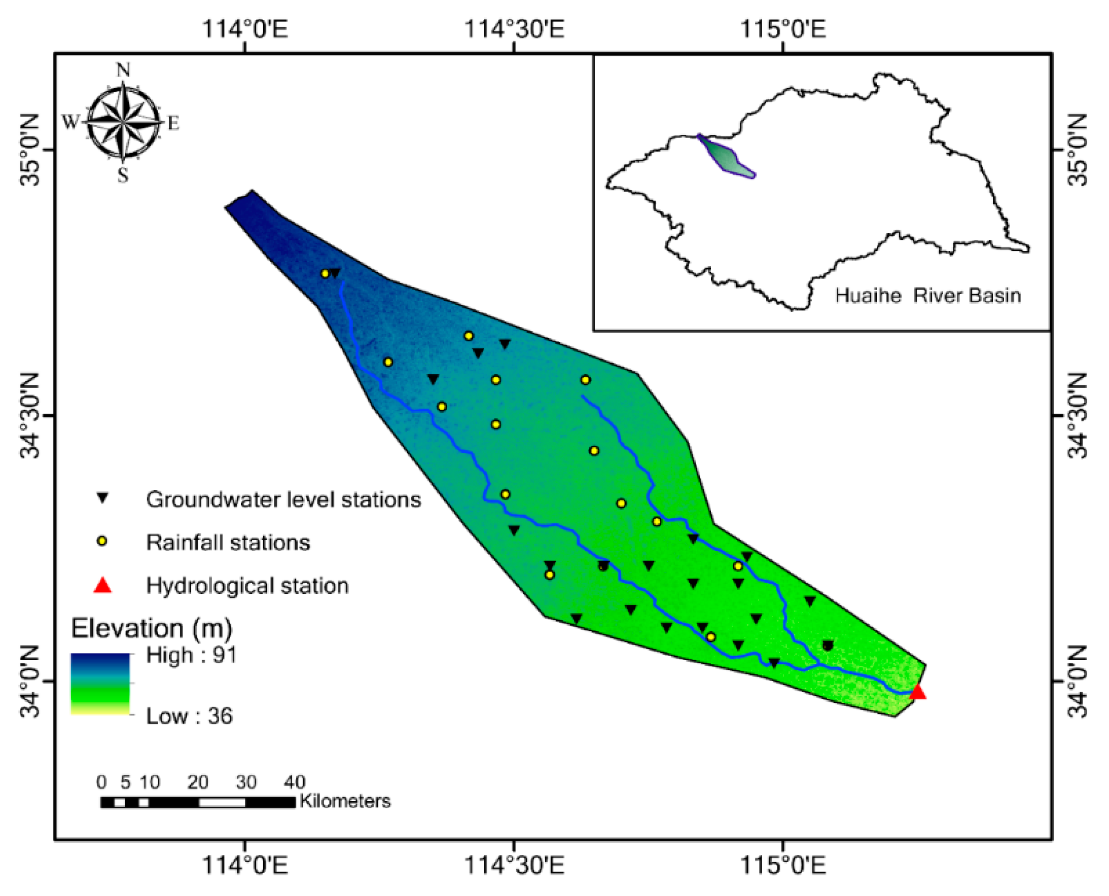
In this study, there are 16 rainfall observation stations, 23 groundwater table monitoring stations and 1 hydrological station recording streamflow discharge at outlet of the catchment. The locations of these stations are shown in Figure 1. In this study, the meteorological, hydrological and 5-day groundwater table data are collected from 2001 to 2009.

3. Methodology

3.1. Development of the Agro-Hydrological Model

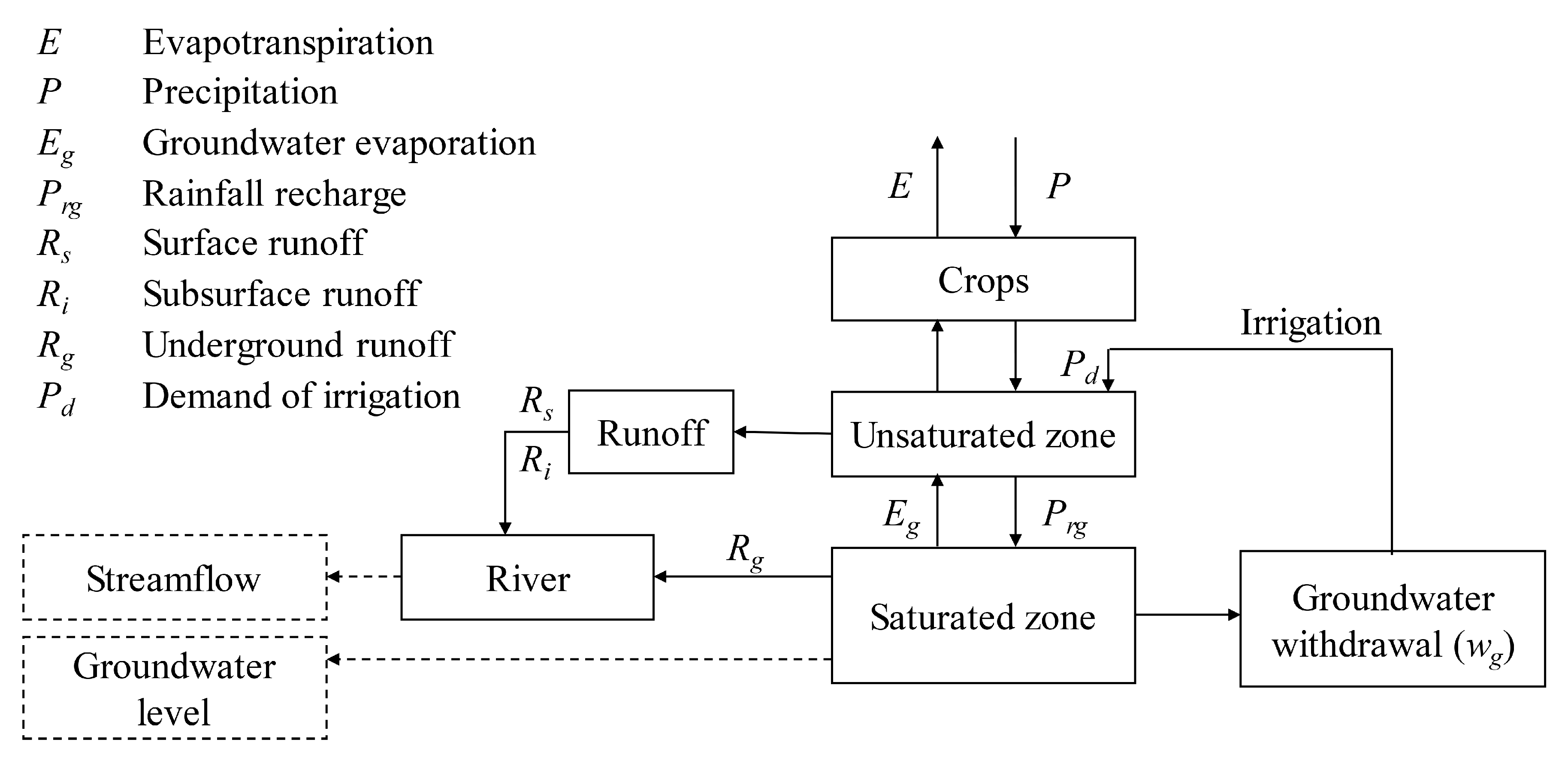
In this study, an agro-hydrological model is developed by integrating agricultural irrigation functions with a hydrological model as illustrated in Figure 2. The model structure is composed of three vertical layers: a crop canopy, an unsaturated zone, and a saturated zone. The net precipitation (P-E) generates surface runoff (R_s), subsurface runoff (R_i), and recharge into the saturated zone (i.e., P_rg). When the phreatic water level exceeds the river water level, groundwater discharges into streamflow (R_g). Due to the capillary action, phreatic water in the saturate zone can supply unsaturated zone through groundwater evaporation (E_g). The irrigation scheme depends on balance of available soil moisture for crop consumption and precipitation infiltration in the root zone. Groundwater withdrawal (W_g) for irrigation is only necessary when available soil moisture cannot meet requirement of crop consumption. Irrigation water is mostly consumed by crops and a small portion recharges into the saturated zone.

3.1.1. Rainfall–Runoff Routing Using the XAJ Model

The Xin’anjiang (XAJ) model has been widely applied to simulate rainfall–runoff response in humid and semi-humid areas in China [24,25,26,27]. The use of a distribution curve to describe uneven distribution of the tension water capacity or field capacity WM is a key concept of the XAJ model:

$$\frac{f}{F}=1-{(1-\frac{WM{\prime }_{}}{WMM})}^B$$

(1)

where f/F is a ratio of the runoff generation area f to the total basin area F, WM′ is a point WM, B is a parameter, and WMM is the maximum value of WM.

So, if $PE\le 0$, runoff R = 0. If $PE>0$ and $PE+A<WMM$, R is equal to:

$$R=PE-WM+W_1+WM{\left[1-\frac{PE+A}{WMM}\right]}^{B+1}$$

(2)

where PE is the net rainfall (P-E), W₁ is the initial soil moisture storage, and A represents the tension water storage state. For $PE+A\ge WMM$, R is equal to:

$$R=PE-WM+W_1$$

(3)

According to water balance in unsaturated zone, the soil moisture storage in the next time step is:

$$W_2=W_1+P{E}_1-R_1$$

(4)

In our model, the separation of the runoff components and flow routing in watersheds and rivers is the same as that in the original XAJ model. Regulation of the catchment heterogeneity for the free water runoff R is represented by a spatial distribution curve of the free water storage capacity with a catchment average SM and an exponent of the spatial distribution curve, EX. For thin soils, SM is around 10 mm, and EX is between 1.0 and 1.5 [19]. The runoff R is then divided into the overland flow R_s, the subsurface flow R_i, and the groundwater flow R_g. The outflow coefficients of the free water storage to interflow and groundwater are denoted by KI and KG. The sum of these two coefficients (KI + KG) may be selected in the range [0.7, 0.8], and the ratio of the three runoff components might be changed by altering the KG/KI ratio [19].

3.1.2. Modifying Evapotranspiration Routing in the XAJ Model

In the original XAJ Model, evapotranspiration is calculated through a three-layer soil moisture scheme. In this study, we focus on modeling the hydrological processes in irrigation regions where evapotranspiration is mainly related to crop growth. The crop evapotranspiration ET_c is estimated according to the FAO 56 guidelines [23]. Under the potential absence of water stress, the crop evapotranspiration ET_c is obtained through multiplying the dual crop coefficients (K_cb + K_e) and the Penman–Monteith reference evapotranspiration rate ET_ref. In particular, following the FAO 56 guidelines, the dual crop coefficients approach splits the crop coefficient K_c into two separate coefficients, namely, a basal crop coefficient K_cb (to account for the plant transpiration) and a soil evaporation coefficient K_e (to account for water evaporation from the soil). Therefore, the crop evapotranspiration ET_c can be expressed as follows:

$$E{T}_c=(K_s\cdot K_{cb}+K_e)\cdot E_{ref}$$

(5)

The Penman–Monteith reference evapotranspiration rate ET_ref [mm/d] can be computed as

$$E_{ref}=\frac{0.408\Delta (R_n-G)+\gamma \frac{900}{T+273}{u}_2(e_s-e_a)}{\Delta +\gamma (1+0.34u_2)}$$

(6)

where R_n [MJ m⁻² d⁻¹] is the net radiation, G [MJ m⁻² d⁻¹] is the soil heat flux, T [°C] and u₂ [m s⁻¹] are the temperature and the wind speed measured at a distance of 2 m, e_s [kPa] is the saturation vapor pressure at air temperature, e_a is the actual vapour pressure, Δ [kPa °C⁻¹] is the slope of the saturation vapor pressure curve, and γ [kPa °C⁻¹] is the psychometric constant at air temperature.

Under limited water supplies, the coefficient K_s in Equation (5) is

$$\{\begin{array}{ll}{K}_{\mathrm{s}}=\frac{TAW-D_r}{TAW-RAW}=\frac{TAW-D_r}{\left(1-\rho \right)TAW}& D_r>RAW\\ K_s=1& D_r\le RAW\end{array}$$

(7)

where TAW [mm] is the total available water, D_r [mm] is the root zone depletion, and RAW [mm] represents the readily available water which can be obtained via multiplying TAW by a depletion coefficient (ρ) to account for the crop water stress resistance. In particular, when water storage in the root zone is equal to RAW, the reduction coefficient K_s becomes 1. The depletion coefficient ρ is a function of the atmospheric evaporative demand and hence can be empirically computed as [21]

$$\rho =\frac{1}{{\alpha }_{\rho }+{\beta }_{\rho }\times E{T}_c}-0.1\times (5-N{O}_{cg})$$

(8)

where ${\alpha }_{\rho }$ and ${\beta }_{\rho }$ [d cm⁻¹] are regression coefficients with values of 0.76 and 1.5, respectively, while NO_cg is the crop group number, which depends on the level of the crop resistance to water stress. The value of the depletion coefficient ρ varies among different crop types. A value of ρ = 0.50 is commonly used [28] for the majority of crop types.

The soil evaporation coefficient, K_e, describes the soil evaporation component of the actual evapotranspiration ET_c. This K_e coefficient is large when the topsoil is wet due to rain or irrigation. By contrast, the K_e coefficient becomes small and tends to zero when the soil surface is dry due to the absence of water in the upper layer. When the topsoil dries out, less water becomes available for evaporation, and consequently, the soil evaporation is reduced in proportion to the amount of water remaining in the soil top layer. Hence, the soil evaporation coefficient K_e can be calculated as

$$K_e=K_r\left(K_{c,\max }-K_{cb}\right)\le f_{ew}{K}_{c,\max }$$

(9)

where K_c,max is the maximum K_c value that is attained immediately after rain or irrigation, K_r is a dimensionless evaporation reduction coefficient that depends on the cumulative depth of water evaporating from the topsoil, and f_ew is the fraction of the exposed wet soil from which most evaporation occurs.

3.1.3. Modifying Groundwater Routing in the XAJ Model

In the original XAJ model, groundwater flow (or base flow) is separated from the free water R, without accounting for groundwater storage routing of the recharge, discharge, and change in storage. In this study, the groundwater balance equation is calculated:

$$\Delta S_{g,t}=P_{rg,t}-R_{g,t}-E_{g,t}-W_{g,t}+Q_g$$

(10)

where P_rg is the rainfall recharge, R_g is the discharge of the groundwater storage (i.e., the base flow), W_g is the amount of groundwater withdrawal, E_g is the groundwater evaporation, Q_g is the water exchange between rivers and aquifers, and ΔS_g is change of the basin average groundwater storage, which can be expressed as:

$$\Delta S_g=\mu (d_1-d_2)$$

(11)

where μ is the specific yield, d₁ and d₂ represent the groundwater depth at the beginning and end of the time period, respectively.

The rainfall recharge, P_rg, is calculated as

$$P_{rg}=(P_{dp}-E_{ref}){\left[\frac{\theta -{\theta }_{wp}}{{\theta }_s-{\theta }_{wp}}\right]}^a$$

(12)

where P_dp is the total of the net precipitation and the irrigation water, θ_s is the saturated moisture, θ_wp is the wilting moisture content, and a is a constant.

The groundwater evaporation, E_g, can be estimated using the Aviriyanover formula [29]:

$$E_g=E_{ref}{(1-\frac{d}{d_{\max }})}^n$$

(13)

where d and d_max are the groundwater depth and the critical water depth (below which groundwater evaporation ceases), respectively, and n is an empirical constant.

Water exchange between rivers and aquifers, Q_g, can be set as

$$Q_g=C_{riv}(d_{riv}-d)$$

(14)

where d_riv is the bottom depth of the river stage, and C_riv represents the hydraulic conductivity between rivers and aquifers.

The spatial distribution of the groundwater depth can be described using the Gamma distribution [30]:

$$f(d_{gw})=\frac{{\lambda }^{\alpha }}{\mathsf{\Gamma }(\alpha )}{d}_{gw}{}^{\alpha -1}{e}^{-\lambda d_{gw}},\alpha >0,\lambda >0$$

(15)

where $\mathsf{\Gamma }(\alpha )$ is the Gamma function, while $\alpha$ and $\lambda$ represent the distribution shape and scale parameters, respectively. The average groundwater depth can be found as the mathematical expectation of the afore-mentioned Gamma-distributed variable, i.e., $\overline{d}=\alpha /\lambda$.

Thus, the groundwater discharge R_g and the groundwater evaporation E_g can be respectively expressed as

$$\begin{array}{l}{R}_g=K{\displaystyle {\int }_{d_{gw=0}}^{d_{gw}=d_{riv}}f(d_{gw})}(d_{riv}-d_{gw})d(d_{gw})\\ \approx \frac{K{(\frac{\alpha }{\overline{d}})}^{\alpha }}{\mathsf{\Gamma }(\alpha )}{\displaystyle \sum _{i=1}^m{e}^{-\frac{\alpha }{\overline{d}}(\frac{i{d}_{riv}}{m})}}{(\frac{i{d}_{riv}}{m})}^{\alpha -1}(d_{riv}-\frac{i{d}_{riv}}{m})\frac{d_{riv}}{m}\end{array}$$

(16)

$$E_g\approx \frac{E_p{(\frac{\alpha }{\overline{d}})}^{\alpha }}{\mathsf{\Gamma }(\alpha )}{\displaystyle \sum _{i=1}^m{e}^{-\frac{\alpha }{\overline{d}}(\frac{i{d}_{\max }}{m})}}{(\frac{i{d}_{\max }}{m})}^{\alpha -1}{(1-\frac{i}{m})}^n\frac{d_{\max }}{m}$$

(17)

where i represents the spatial location of the groundwater depth.

3.2. Construction of Multi-Objective Functions for Parameter Calibration

In this work, we use the optimization function proposed by Cheng et al. [31] to calibrate the parameters of the modified XAJ model. The objective function is obtained as follows.

The error (e) between the simulated and the observed variable at time step i can be expressed as

$$e_{i,y}=ob{s}_{i,y}-si{m}_{i,y}$$

(18)

where $ob{s}_{i,y}$ and $si{m}_{i,y}$ are the observed and the simulated outcomes, respectively, at time step i. Assume that the errors are independent and identically distributed, each error $e_{i,y}$ can be modeled with a Gaussian-distributed random variable, whose probability density function is:

$$p\left(e_{i,y}|\theta \right)=\frac{1}{\sqrt{2\pi {\sigma }_y}}\exp \left(-\frac{e_{i,y}{}^2}{2{\sigma }_y{}^2}\right)$$

(19)

where ${\sigma }_y$ is the standard deviation, and θ represents a parameter set.

The log-likelihood function of y is as follows:

$$l_y\left(\theta |ob{s}_y\right)=\ln \left({\displaystyle {\prod }_1^{n}p\left(e_{i,y}|\theta \right)}\right)=-\frac{n}{2}\ln \left(2\pi \right)-\frac{n}{2}\ln \left({\sigma }_y{}^2\right)-{\displaystyle {\sum }_1^n\frac{e_{i,y}^2}{2{\sigma }_y{}^2}}$$

(20)

where n is the length of the error time series.

When ${\sigma }_y{}^2={\displaystyle {\sum }_1^n{e}_{i,y}^2/n}$ is the unbiased estimator of ${\sigma }_y{}^2$, $l_y\left(\theta |ob{s}_y\right)$ reaches its maximum value:

$$\begin{array}{ll}\max \left(l_y\left(\theta |ob{s}_y\right)\right)& =-\frac{n}{2}\ln \left(2\pi \right)-\frac{n}{2}\ln \left({\sigma }_y{}^2\right)-\frac{n}{2}\\ & =-\frac{n}{2}\ln \left(2\pi \epsilon \right)-\frac{n}{2}\ln \left({\displaystyle {\sum }_1^n\frac{e_{i,y}^2}{n}}\right)\end{array}$$

(21)

where ε is used herein to denote the base of the natural logarithms, $\epsilon \approx 2.718$.

The single-objective function of the Nash-Sutcliffe efficiency for y (NSE_y) [32] is expressed as

$$NS{E}_y=1-\frac{{\displaystyle {\sum }_1^n{\left(si{m}_{i,y}-ob{s}_{i,y}\right)}^2}}{{\displaystyle {\sum }_1^n{\left(ob{s}_{i,y}-\overline{ob{s}_y}\right)}^2}}=1-\frac{{\displaystyle {\sum }_1^n{e}_{i,y}{}^2}}{{\displaystyle {\sum }_1^n{\left(ob{s}_{i,y}-\overline{ob{s}_y}\right)}^2}}$$

(22)

where $\overline{ob{s}_y}$ is the mean observed outcome. From Equation (21), we can obtain

$${\displaystyle {\sum }_1^n\frac{e_{i,y}^2}{n}}=\frac{n-1}{n}\left(1-NS{E}_y\right){\sigma }_y^2$$

(23)

By substituting Equation (22) into Equation (20), the log-likelihood function of Equation (20) is transformed into

$$\max \left(l_y\left(\theta |ob{s}_y\right)\right)=-\frac{n}{2}\ln \left(2\pi \epsilon \frac{n-1}{n}{\sigma }_y^2\right)-\frac{n}{2}\ln \left(1-NS{E}_y\right)$$

(24)

Assuming that the simulation errors for discharge $e_{i,Q}$ and the groundwater depth $e_{i,D}$ are independent of each other, the following multi-objective function NSE_union can be constructed by combining the Nash–Sutcliffe efficiency coefficient of river discharge (NSE_flow) and the Nash–Sutcliffe efficiency coefficient of groundwater depth (NSE_depth):

$$l\left(\theta |obs\right)=l_{flow}\left(\theta |ob{s}_{flow}\right)+l_{depth}\left(\theta |ob{s}_{depth}\right)$$

(25)

The term $-\frac{n}{2}\ln \left(2\pi \epsilon \frac{n-1}{n}{\sigma }_y^2\right)$ in Equation (24) is constant, and hence, the multi-objective function of Equation (25) can be rewritten as

$$l^{\prime }\left(\theta |obs\right)=-\frac{n}{2}\ln \left(1-NS{E}_{flow}\right)-\frac{m}{2}\ln \left(1-NS{E}_{depth}\right)$$

(26)

3.3. Sensitivity Analysis and Model Calibration

The Monte-Carlo Analysis Tool (MCAT) [33] is an effective sensitively analysis tool based on the generalized likelihood uncertainty estimation (GLUE) [34], which can repeatedly simulate valid parameter groups in physical or conceptual scopes. In this study, the shuffled complex evolution (SCE-UA) algorithm is further used to calibrate the sensitive parameters. The SCE-UA algorithm has the advantages of fewer parameters and efficient operation [35]. The details of the SCE-UA algorithm are given by Duan et al. [16].

4. Results and Discussion

4.1. Model Sensitivity Analysis, Calibration and Verification

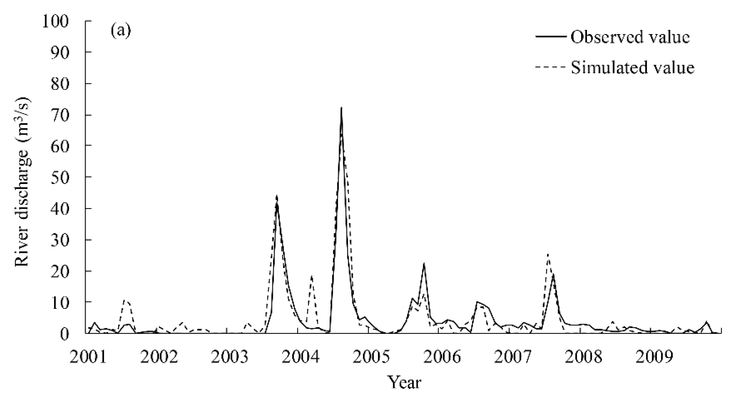
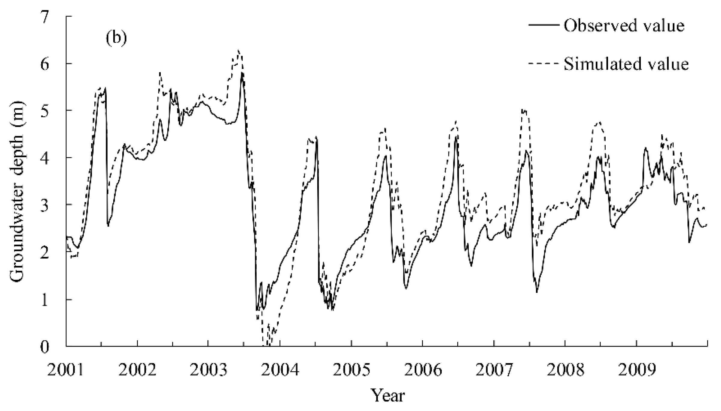
The proposed agro-hydrological model inputs meteorological data and crop types, the simulated results include several hydrological components, such as crop evapotranspiration, streamflow, and groundwater tables. The model has 17 model parameters (shown in

Table 2. The model parameters and calibration results.

Module	Parameters	Meaning of Parameters	Initial Value	Objective Functions
				NSEflow	NSEdepth	NSEunion
Runoff Generation	B	Exponent of the tension water capacity distribution curve	0.4	0.449	0.405	0.429
	RN	Vadose zone thickness/m	1.85	1.746	1.852	2.126
Runoff Separation	SM	Areal mean free water capacity/mm	15.5	13.45	13.81 ☆	17.37
	EX	Exponent of the free water storage capacity distribution curve	1.6	1.6 ☆	1.6 ☆	1.6 ☆
	KI	Outflow coefficients of interflow (KI + KG = 0.7)	0.25	0.21 ★	0.34	0.19 ★
Flow Concentration	EI	Recession constant of interflow storage	0.88	0.88 ☆	0.88 ☆	0.88 ☆
	C1	Muskingum parameter	0.88	0.893 ★	0.887	0.877 ★
	C2	Muskingum parameter	0.1	0.089 ★	0.082 ★	0.085 ★
Groundwater Evaporation	n	Coefficient of groundwater evaporation	1.6	1.6 ☆	1.58	1.6 ☆
	driv	Maximum cutting depth of river	1.9	2.277 ★	2.028 ★	1.955
	dmax	Critical depth to groundwater	5	4.660 ★	4.256 ★	4.030 ★
Groundwater reservoir	a	Coefficient for groundwater recharge	0.6	0.493 ★	0.488 ★	0.659
	K	Baseflow coefficient	0.024	0.024 ☆	0.024 ☆	0.024 ☆
	QC	Coefficient of groundwater withdrawal amount	0.65	0.633	0.746 ★	0.743
	γ	Gamma curve shape parameter	2.8	2.927	3.118 ★	3.290 ★
	μ	Specific yield	0.055	0.065 ★	0.062 ★	0.062 ★
The optimal values of objective functions	NSEflow	Calibration period		0.62	0.46	0.55
		Validation period		0.51	0.18	0.40
	NSEdepth	Calibration period		−0.82	0.94	0.92
		Validation period		−0.13	0.69	0.58

Note: ^★ represents sensitive parameters, ^☆ represents insensitive parameters.

). By normalizing the likelihood function, the sensitive and insensitive parameters are identified according to the single-objective functions NSE_flow and NSE_depth, as well as the multi-objective function NSE_union. The sensitive parameters are calibrated against the observed streamflow and groundwater depth from 2001 to 2004 using the SCE-UA algorithm. The model is validated for the period from 2005 to 2009. The optimal parameter settings are listed in Table 2, and the simulation results are shown in Figure 3, Figure 4 and Figure 5.

As shown in Table 2, C₂, d_max, and μ are all sensitive parameters, while EX, EI, and K are all insensitive ones. Also, the parameters KI and C₁ are sensitive to the streamflow objective function, and insensitive to the objective function of the groundwater depth. As well, the parameters QC and γ are insensitive to the streamflow objective function and sensitive to groundwater-depth objective function. C₂ and μ are both sensitive to the streamflow and groundwater-depth objective functions. The parameters that are insensitive to the single-objective functions are also insensitive to the multi-objective function.

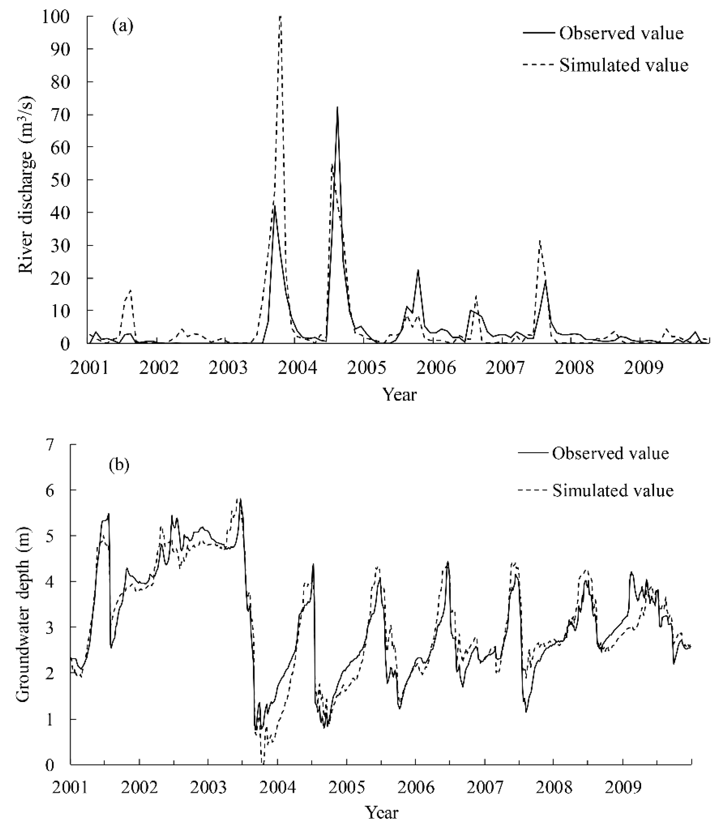
Using the calibrated parameters of Table 2, a comparison of the simulation results is shown in

Table 3. Comparison of the simulated and observed results of the discharge and the groundwater depth from 2001 to 2009.

Year	Discharge (m3/s)				Groundwater Depth (m)
	Observed Value	Simulation			Observed Value	Simulation
		NSEflow	NSEdepth	NSEunion		NSEflow	NSEdepth	NSEunion
2001	1.17	2.18	3.14	1.74	3.49	3.70	3.44	3.44
2002	0.02	1.05	1.63	0.94	4.70	4.95	4.55	4.45
2003	8.28	9.66	18.73	14.32	3.46	3.61	3.38	3.35
2004	13.27	16.63	12.93	16.61	2.17	2.09	2.02	2.01
2005	5.00	3.49	3.02	4.02	2.42	2.78	2.54	2.62
2006	4.23	2.97	1.92	1.71	2.58	3.16	2.79	2.94
2007	4.78	4.53	5.18	3.98	2.54	3.17	2.79	2.98
2008	1.36	0.78	0.80	0.33	3.04	3.48	3.09	3.23
2009	0.75	0.70	1.08	0.42	3.27	3.57	3.17	3.32
average	4.31	4.66 (8.1%)	5.38 (24.7%)	4.90 (13.5%)	3.07	3.39 (10.4%)	3.09 (0.1%)	3.15 (2.6%)

for different objectives. The simulated and observed discharge values agree well when the discharge is used as a single objective (Figure 3a). The Nash efficiency coefficients (NSE_flow) of the calibration and validation periods are 0.62 and 0.51, respectively. On average, maximizing NSE_flow yields the minimum difference of 8.1% between the simulated and observed discharges. The single-objective NSE_flow function mainly reflects rainfall–runoff response but fails to estimate the groundwater depth. Figure 3b shows significant errors between the simulated and observed groundwater depths. However, the simulation error is large for the groundwater depth with the maximum difference of 10.4% between the simulated and observed groundwater depths. When the groundwater depth is used as a single objective, the single-objective NSE_depth function can better simulate changes in the groundwater depth Figure 4b. The NSE_depth values of the calibration and validation periods are 0.94 and 0.69, respectively. However, it cannot accurately simulate the rainfall-runoff response in the flood periods. Figure 4a indicates that the model significantly overestimates the flood peak in 2003 while it underestimates the flood peak in 2004. Maximizing NSE_depth produces the maximum difference of 24.7% between the simulated and observed discharges on average.

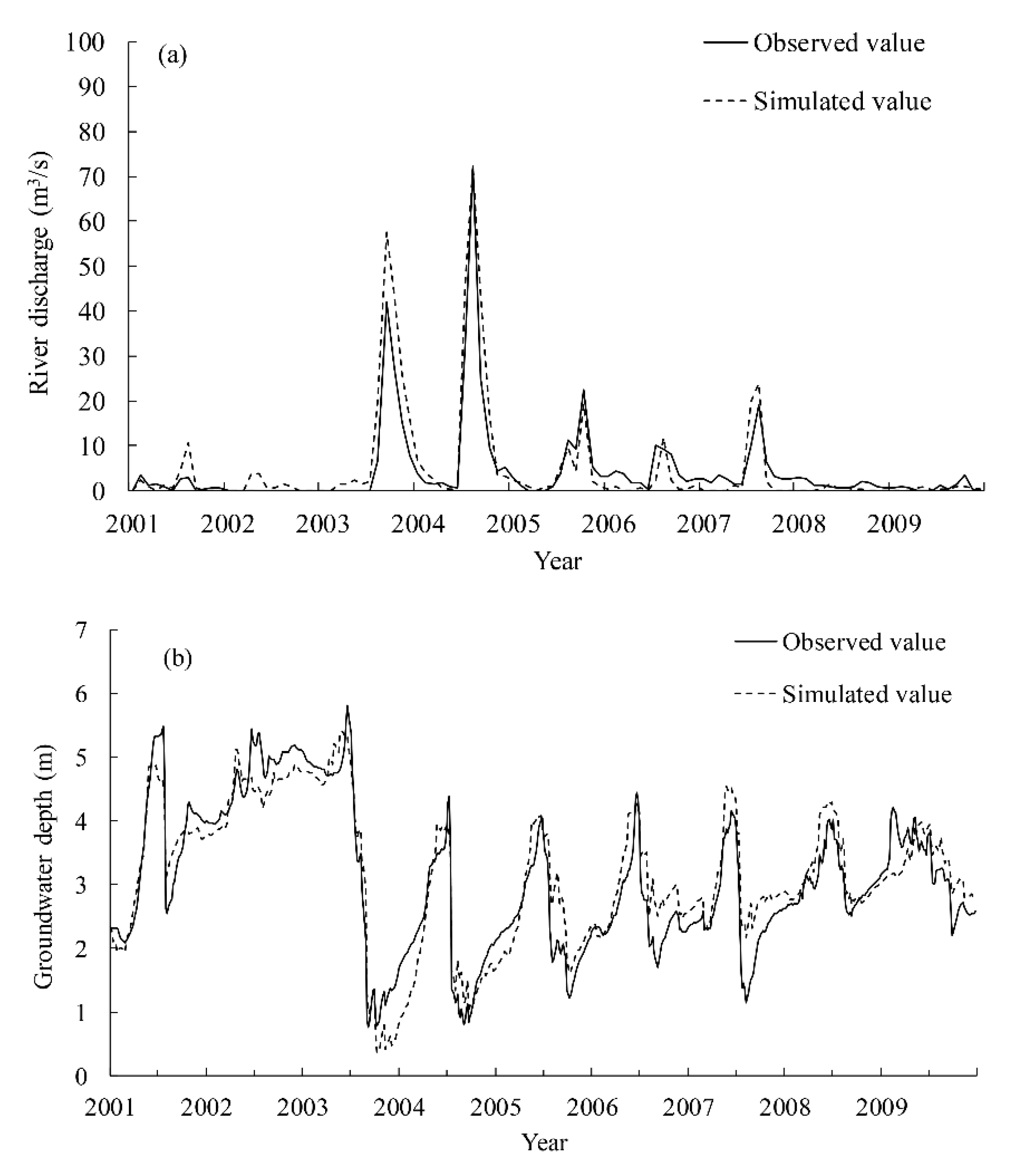
Maximizing the multi-objective function NSE_union achieves a balance between the two single-objective extremes. Indeed, the simulation errors of the discharge and the groundwater depth for the calibration and validation periods fall in the middle range for the three parameter sets. As shown in Table 2, the multi-objective formulation results in NSE_flow and NSE_depth values of 0.55 and 0.92, respectively, during the calibration period. The corresponding values during the validation period are 0.40 and 0.58, respectively. The associated simulation errors of the average discharge and the groundwater depth are 13.5% and 2.6%, respectively. Figure 5 shows consistency in the simulated discharge and groundwater depth using the multi-objective function. As the basin conditions are somewhat influenced by human activities, the agro-hydrological model can be employed to balance the simulation outcomes in terms of the discharge and the groundwater depth. Therefore, the multi-objective optimization results are used for the next analyses.

4.2. Estimation of the Groundwater Use for Irrigation

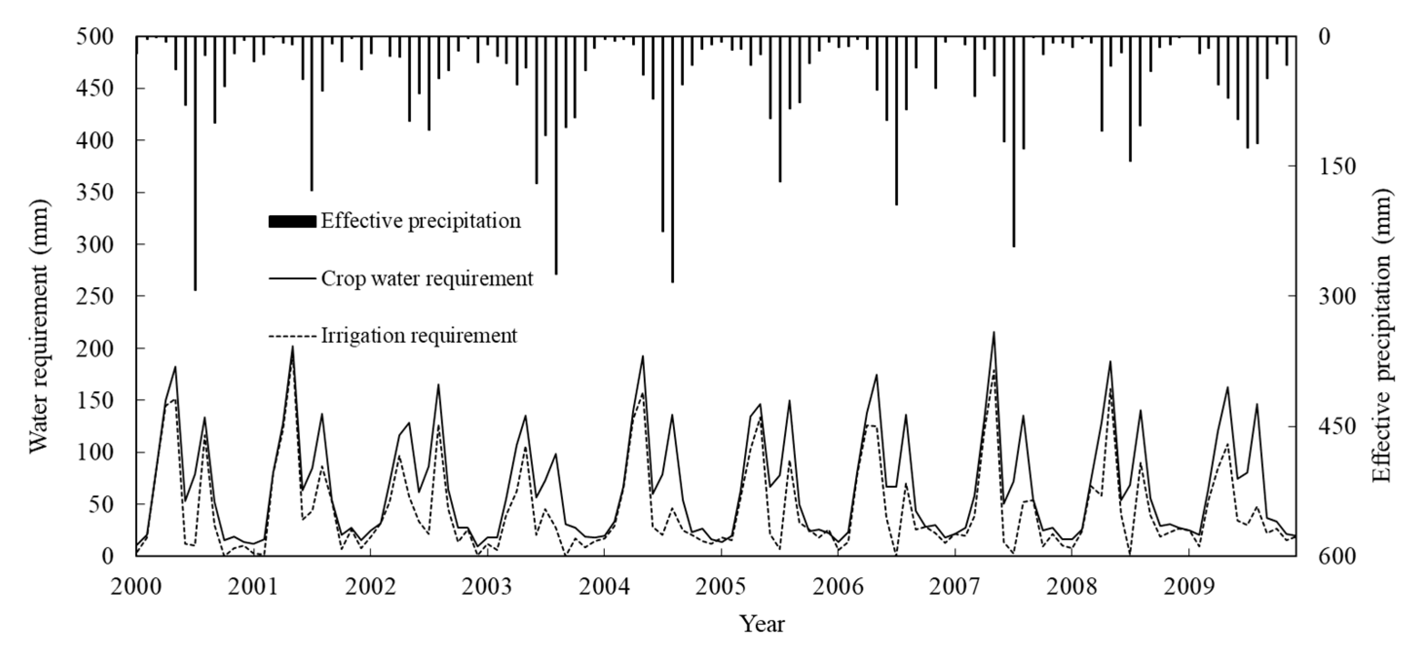
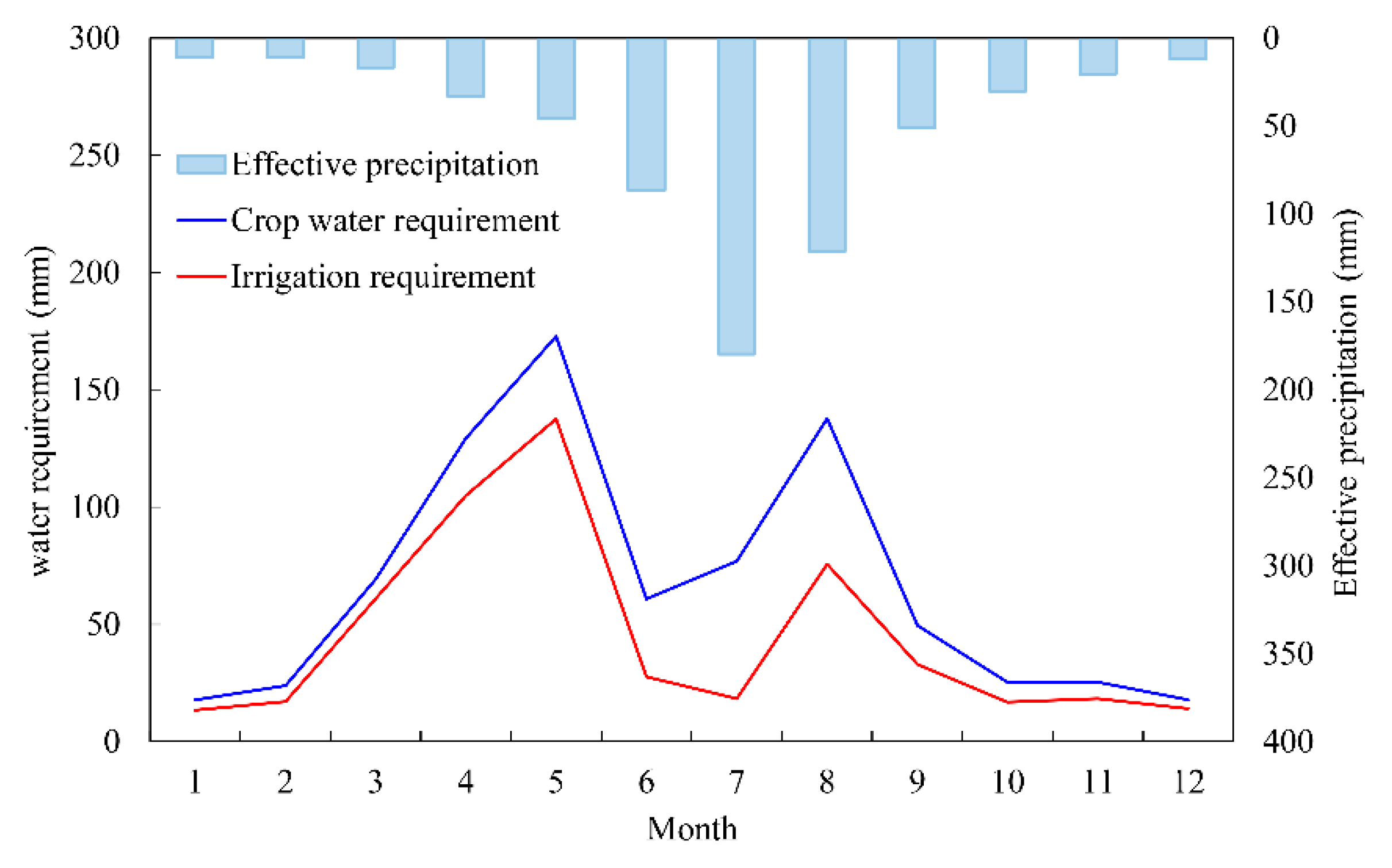
Figure 6 shows the annual effective precipitation (PE = P − E), the crop water demand (ET_c), and the irrigation demand (Wg) of the Xuanwu basin from 2000 to 2009. When the effective precipitation is not enough to meet the demand of crop evapotranspiration, then supplementary irrigation is needed. Therefore, the irrigation demand is the difference between the crop water demand and the effective precipitation in the growth period. As shown by Figure 6, irrigation is necessary for crop growth in the study area. Changes in the irrigation demand are consistent with those of the crop water demand. Figure 7 reflects changes in the monthly irrigation water demand for the winter wheat and summer maize. From transition of month 6 to 8, instead of high precipitation, crop water requirement is high. It is due to crop physiological stage of summer maize (peak vegetative growth around tasseling, Table 1).

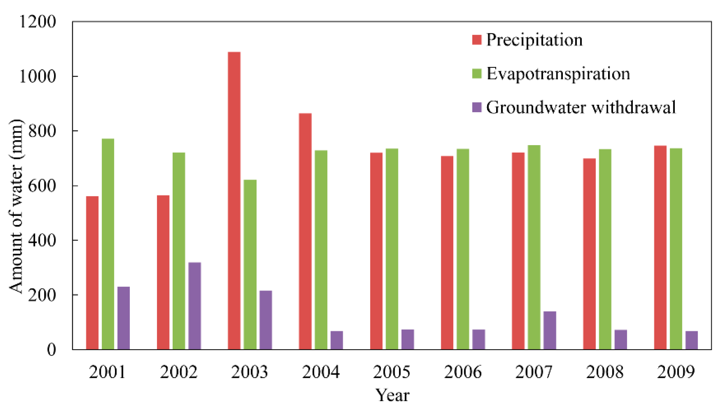
Figure 8 shows that the annual groundwater withdrawal is significantly affected by precipitation and evapotranspiration. In fact, the groundwater withdrawal is large if the precipitation is small and the evapotranspiration is large. For example, in the years of 2001 and 2002, precipitation levels were 560 and 564 mm, respectively. The corresponding evapotranspiration levels were 771 and 721 mm, respectively, while the amounts of groundwater withdrawal levels were 230 and 319 mm, respectively. In the years of 2004 and 2009, precipitation was larger than evaporation, and the exploitations were only 68 mm and 69 mm, respectively. However, in 2003, precipitation was much higher than evapotranspiration, but the groundwater withdrawal was still high. These patterns could be attributed to large floods (with high rainfall from June to September) in the Huaihe River in the summer of 2003 and low rainfall from March to May, when the crop water demand is large.

The groundwater withdrawal is given for each of four stages in the whole growth period of winter wheat and summer maize shown in

Table 4. The length of each growth period and the groundwater withdrawal for winter wheat and summer maize crops.

Crop	Project	Initial Stage	Crop Development Stage	Mid-Season Stage	Late Season Stage	Whole Growth Period
Winter wheat	Growth period (days)	60	70	67	44	241
	Groundwater withdrawal (mm)	5	4.7	81.2	49.6	140.5
Summer maize	Growth period (days)	20	20	31	51	122
	Groundwater withdrawal (mm)	0	3	6.2	4.5	13.7

. Clearly, the groundwater withdrawal for winter wheat irrigation at the mid-season stage is the largest (accounting for 57.8% among the four growth stages). The groundwater withdrawal used for summer maize irrigation is much smaller than that of winter wheat. Moreover, the irrigation during the mid-season and late-season stages consumes most of the groundwater withdrawal compared with other stages.

Estimates of the monthly average groundwater withdrawal for winter wheat and summer maize crops are shown in Figure 9. The groundwater withdrawal for winter wheat in May is the largest, accounting for 42.7% of the total wheat irrigation amount in the whole growth period. The growth period for summer maize is generally from the middle of June to the middle of September. Since there is enough precipitation during this period, the irrigation water demand for maize is significantly smaller than that of wheat.

4.3. Correlation between the Groundwater Withdrawal for Irrigation and the Groundwater Level

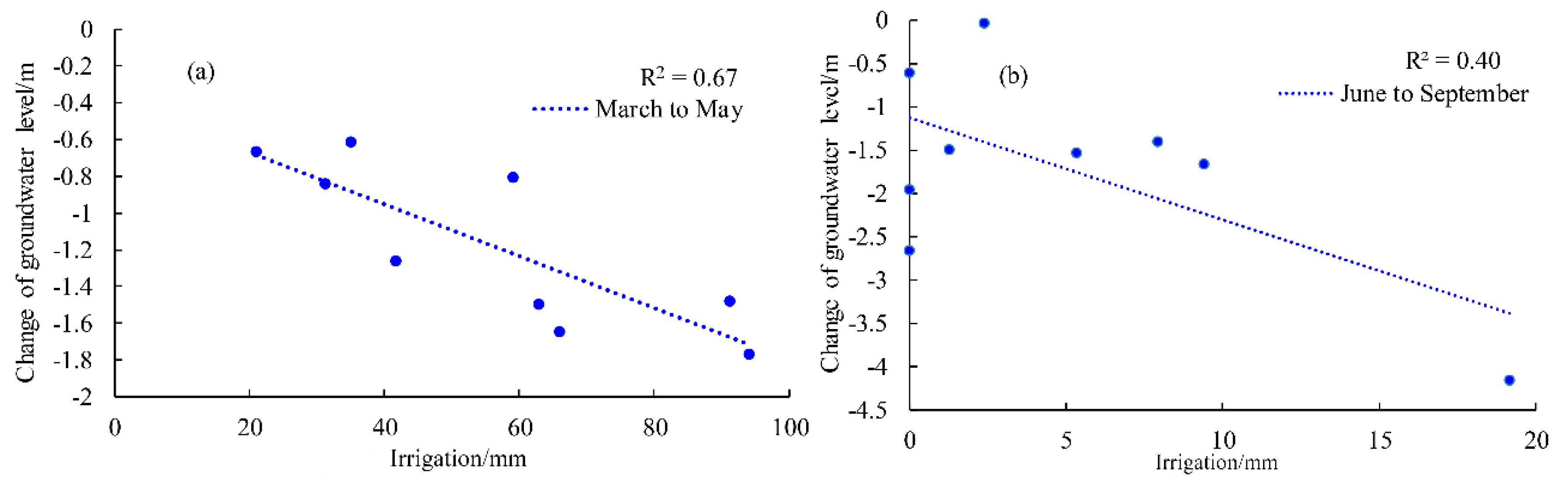
Based on the estimated groundwater withdrawal for irrigation and change in the observed groundwater level, the correlation between these variables during the growth periods of winter wheat and summer maize is presented in Figure 10.

There is little precipitation during the March-to-May period which represents the main growth season of winter wheat. Thus, it is difficult to meet the crop water demand during this period unless groundwater is exploited for irrigation. Figure 10a shows that there is a significant negative correlation between the change in the groundwater level and the groundwater withdrawal. The June-to-September period is the growth season of summer maize, during which precipitation is relatively abundant, and the irrigation water demand for summer maize is relatively small. As shown in Figure 10b, the negative correlation between the groundwater level change and the groundwater withdrawal is relatively weak.

4.4. Precipitation Effects on Irrigation, Streamflow, and the Groundwater Depth

We show here results of numerical experiments for investigating the effects of precipitation on irrigation, streamflow, and groundwater depth. For this purpose, the precipitation is systematically reduced by 1%, 3%, and 5%. We run the agro-hydrological model repeatedly for each precipitation scenario. The simulation results are shown in

Table 5. Effects of precipitation variability on irrigation, streamflow, and the groundwater tables.

Variation of Precipitation (%)	Irrigation Water Requirement (mm) (%)	Groundwater Withdrawal (mm) (%)	Average Annual Groundwater Depth (m) (%)	Average Annual Runoff (mm) (%)
0%	99.6	63.1	3.15	30.6
−1%	105.3 (5.7%)	66.7 (5.7%)	3.21 (1.9%)	29.1 (−4.9%)
−3%	122.3 (22.8%)	77.4 (22.7%)	3.30 (4.8%)	26.9 (−12.1%)
−5%	138.8 (39.4%)	87.9 (39.3%)	3.43 (8.9%)	23.3 (−23.9%)

. When the total precipitation is reduced by 5% while the model parameters are kept unchanged, the average annual runoff decreases by 23.9%, the irrigation water demand and the groundwater withdrawal increase by 39.4% and 39.3%, respectively, and the average groundwater depth increases by 8.9%. The precipitation reduction directly results in runoff reduction as well as an increase in the irrigation water demand. Furthermore, the increase of the groundwater withdrawal leads to a higher groundwater depth, and further affects the runoff level. The results indicate that the precipitation variations have significant effects on the runoff and groundwater withdrawal. Indeed, hydrological variables and groundwater withdrawal are highly interconnected in groundwater-irrigated regions. Precipitation is the driving factor of the whole system, and it not only affects the hydrological variables but also greatly influences irrigation activities. Meanwhile, these activities also have direct impacts on hydrological variables, such as groundwater tables.

5. Conclusions

As the Chinese government promotes the sustainable use of groundwater resources and prevents groundwater over-exploitation, estimation of groundwater withdrawal in irrigated fields is quite important for effective control of groundwater utilization in an appropriate level. In this study, the agro-hydrological model is developed for estimating the annual, seasonal, and monthly variations of groundwater withdrawal and other hydrological components in an irrigated area. To avoid the limitations of single-objective parameter calibration methods, we established a multi-objective optimization approach that involves objectives of flow discharge and groundwater depth.

The results show that single-objective parameter calibration methods cannot effectively simulate the dynamics of the river discharge and the groundwater depth at the same time. By contrast, the simulation results of the multi-objective parameter calibration method for a specific objective function are not as good as those of single-objective optimization. Nevertheless, multi-objective parameter calibration can achieve high accuracy in simulating simultaneous changes of the river discharge and the groundwater depth. For the wheat-maize cropping system in the study, the estimated average annual groundwater withdrawal for irrigation is about 140.5 mm for wheat and 13.7 mm for maize. The wheat irrigation is in the range of 87–307 mm as estimated by the water resource balance in the whole Huaihe River Basin. Alternatively, this irrigation is 180 mm according to the Yucheng Comprehensive Experimental Station of the Chinese Academy of Sciences in the Shangdong Province, where the annual precipitation of 600 mm is close to that in our study catchment [36]. Moreover, the simulated seasonal variations of the irrigation amount are dependent on precipitation and crop types. For example, the groundwater withdrawal for irrigation of winter wheat is much larger than that of summer maize. Correlation analysis between the groundwater withdrawal for irrigation and change in the groundwater depth in the crop-growing season shows that groundwater withdrawal is the dominant factor for the groundwater depth change in the considered basin. In addition, the negative correlation between the groundwater depth change and the groundwater withdrawal is more significant in the winter wheat season than in the summer maize season.

Since the Huaihe River catchment is located in a transition zone of semi-humid and semi-arid climate, short-term and long-term precipitation variations are observed. This phenomenon significantly affects crop irrigation and hydrological components. In this study, results of numerical modeling experiments show that as the precipitation is systematically reduced by 1–5%, the irrigation water demand and the groundwater withdrawal increase by 39.4% and 39.3%, respectively. The combined effects of the reduced precipitation and the increased groundwater withdrawal would lead to a decrease of the average annual runoff by 23.9% and to an increase of the average groundwater depth by 8.9%.

This model can be applied in basins where groundwater withdrawal is unknown or well-pumping data is incomplete. Using both the streamflow discharge and the groundwater tables to calibrate model parameters can reduce the uncertainty of the simulated hydrological components and also balance water storage in unsaturated and saturated zones. However, with the high numbers of model parameters and hydrological variables for this kind of complex models, more detailed data could be further collected and analyzed to increase the reliability of the simulation results.

References

- FAO (Food and Agriculture Organization of the United Nations). AQUASTAT Main Database; FAO (Food and Agriculture Organization of the United Nations): Rome, Italy, 2016. [Google Scholar]
- Siebert, S.; Burke, J.; Faures, J.M.; Frenken, K.; Hoogeveen, J.; Döll, P.; Portmann, F.T. Groundwater use for irrigation—a global inventory. Hydrol. Earth Syst. Sci. 2010, 14, 1863–1880. [Google Scholar] [CrossRef] [Green Version]
- Maréchal, J.; Dewandel, B.; Ahmed, S.; Galeazzi, L.; Zaidi, F.K. Combined estimation of specific yield and natural recharge in a semi-arid groundwater basin with irrigated agriculture. J. Hydrol. 2006, 329, 281–293. [Google Scholar] [CrossRef] [Green Version]
- Amri, R.; Zribi, M.; Chabaane, Z.L.; Szczypta, C.; Calvet, J.C.; Boulet, G. FAO-56 dual model combined with multi-sensor remote sensing for regional evapotranspiration estimations. Remote. Sens. 2014, 6, 5387–5406. [Google Scholar] [CrossRef] [Green Version]
- Cruz-Blanco, M.; Lorite, I.; Santos, C. An innovative remote sensing based reference evapotranspiration method to support irrigation water management under semi-arid conditions. Agric. Water Manag. 2014, 131, 135–145. [Google Scholar] [CrossRef]
- Alcamo, J.; Flörke, M.; Maerker, M. Future long-term changes in global water resources driven by socio-economic and climatic changes. Hydrol. Sci. J. 2007, 52, 247–275. [Google Scholar] [CrossRef]
- Wada, Y.; Wisser, D.; Bierkens, M.F. Global modeling of withdrawal, allocation and consumptive use of surface water and groundwater resources. Earth Syst. Dynam. 2014, 5, 15–40. [Google Scholar] [CrossRef] [Green Version]
- Wisser, D.; Frolking, S.; Douglas, E.M.; Fekete, B.M.; Schumann, A.H.; Vörösmarty, C.J. The significance of local water resources captured in small reservoirs for crop production—A global-scale analysis. J. Hydrol. 2010, 384, 264–275. [Google Scholar] [CrossRef] [Green Version]
- Liu, J. A GIS-based tool for modelling large-scale crop-water relations. Environ. Model. Softw. 2009, 24, 411–422. [Google Scholar] [CrossRef]
- Lapola, D.M.; Priess, J.A.; Bondeau, A. Modeling the land requirements and potential productivity of sugarcane and jatropha in Brazil and India using the LPJmL dynamic global vegetation model. Biomass Bioenergy 2009, 33, 1087–1095. [Google Scholar] [CrossRef]
- Van Dam, J.C.; Huygen, J.; Wesseling, J.; Feddes, R.; Kabat, P.; van Walsum, P.; Groenendijk, P.; van Diepen, C. Theory of SWAP Version 2.0, Simulation of Water Flow, Solute Transport and Plant Growth in the Soil-Water-Atmosphere-Plant Environment; DLO Winand Staring Centre: Wageningen, The Netherlands, 1997. [Google Scholar]
- Gassman, P.W.; Reyes, M.R.; Green, C.H.; Arnold, J.G. The soil and water assessment tool: Historical development, applications, and future research directions. Trans. ASABE 2007, 50, 1211–1250. [Google Scholar] [CrossRef] [Green Version]
- Duan, Q.; Gupta, H.V.; Sorooshian, S.; Rousseau, A.N.; Turcotte, R. Calibration of Watershed Models; American Geophysical Union: Washington, DC, USA, 2004. [Google Scholar]
- Ye, L.; Zhou, J.; Zeng, X.; Guo, J.; Zhang, X. Multi-objective optimization for construction of prediction interval of hydrological models based on ensemble simulations. J. Hydrol. 2014, 519, 925–933. [Google Scholar] [CrossRef]
- Fereidoon, M.; Koch, M. SWAT-MODSIM-PSO optimization of multi-crop planning in the Karkheh River Basin, Iran, under the impacts of climate change. Sci. Total. Environ. 2018, 630, 502–516. [Google Scholar] [CrossRef]
- Adeyeri, O.; Laux, P.; Arnault, J.; Lawin, A.; Kunstmann, H. Conceptual hydrological model calibration using multi-objective optimization techniques over the transboundary Komadugu-Yobe basin, Lake Chad Area, West Africa. J. Hydrol. Reg. Stud. 2020, 27, 100655. [Google Scholar] [CrossRef]
- Vrugt, J.A.; Gupta, H.; Bastidas, L.A.; Bouten, W.; Sorooshian, S. Effective and efficient algorithm for multiobjective optimization of hydrologic models. Water Resour. Res. 2003, 39. [Google Scholar] [CrossRef] [Green Version]
- Lakshimi, G.; Sudheer, K. Parameterization in hydrological models through clustering of the simulation time period and multi-objective optimization based calibration. Environ. Model. Softw. 2021, 138, 104981. [Google Scholar] [CrossRef]
- Ren-Jun, Z. The Xinanjiang model applied in China. J. Hydrol. 1992, 135, 371–381. [Google Scholar] [CrossRef]
- Mo, X.-G.; Hu, S.; Lin, Z.-H.; Liu, S.-X.; Xia, J. Impacts of climate change on agricultural water resources and adaptation on the North China Plain. Adv. Clim. Chang. Res. 2017, 8, 93–98. [Google Scholar] [CrossRef]
- Wang, Z.L.; Zhang, Q.B.; Li, R. Experimental Study on Hydrology in Huaibei Plain; China University of Science and Technology Press: Shanghai, China, 2011. [Google Scholar]
- Cheng, X.; Yu, M.; Zhang, J. Comparative study on hydrogeological conditions of Huaihe mining area. J. Geogr. Cartogr. 2018, 1. [Google Scholar] [CrossRef]
- Allen, R.G.; Pereira, L.S.; Raes, D.; Smith, M. Crop Evapotranspiration—Guidelines for Computing Crop Water Requirements-FAO Irrigation and Drainage Paper 56; FAO (Food and Agriculture Organization of the United Nations): Rome, Italy, 1998. [Google Scholar]
- Yao, C.; Zhang, K.; Yu, Z.; Li, Z.; Li, Q. Improving the flood prediction capability of the Xinanjiang model in ungauged nested catchments by coupling it with the geomorphologic instantaneous unit hydrograph. J. Hydrol. 2014, 517, 1035–1048. [Google Scholar] [CrossRef]
- Song, X.-M.; Kong, F.-Z.; Zhan, C.-S.; Han, J.-W. Hybrid optimization rainfall-runoff simulation based on Xinanjiang model and artificial neural network. J. Hydrol. Eng. 2012, 17, 1033–1041. [Google Scholar] [CrossRef]
- Lu, M.; Li, X. Time scale dependent sensitivities of the XinAnJiang model parameters. Hydrol. Res. Lett. 2014, 8, 51–56. [Google Scholar] [CrossRef] [Green Version]
- Hao, F.; Sun, M.; Geng, X.; Huang, W.; Ouyang, W. Coupling the Xinanjiang model with geomorphologic instantaneous unit hydrograph for flood forecasting in northeast China. Int. Soil Water Conserv. Res. 2015, 3, 66–76. [Google Scholar] [CrossRef] [Green Version]
- Van Diepen, C.; Rappoldt, C.; Wolf, J.; van Keulen, H. Crop Growth Simulation Model WOFOST. Documentation Version 4.1; Centre for World Food Studies: Wageningen, The Netherlands, 1988. [Google Scholar]
- Verianov, A. The Level Drainage Facilities to Control the Irrigation Salinization; China Industry Press: Beijing, China, 1963. [Google Scholar]
- Yeh, P.J.-F.; Eltahir, E.A.B. Representation of water table dynamics in a land surface scheme. Part I: Model development. J. Clim. 2005, 18, 1861–1880. [Google Scholar] [CrossRef]
- Cheng, Q.-B.; Chen, X.; Xu, C.-Y.; Reinhardt-Imjela, C.; Schulte, A. Improvement and comparison of likelihood functions for model calibration and parameter uncertainty analysis within a Markov chain Monte Carlo scheme. J. Hydrol. 2014, 519, 2202–2214. [Google Scholar] [CrossRef]
- Nash, J.E.; Sutcliffe, J.V. River flow forecasting through conceptual models part I—A discussion of principles. J. Hydrol. 1970, 10, 282–290. [Google Scholar] [CrossRef]
- Beven, K.J.; Binley, A. The future of distributed models: Model calibration and uncertainty prediction. Hydrol. Process. 1992, 6, 279–298. [Google Scholar] [CrossRef]
- Beven, K.J.; Kirkby, M.J. A physically based, variable contributing area model of basin hydrology/Un modèle à base physique de zone d’appel variable de l’hydrologie du bassin versant. Hydrol. Sci. J. 1979, 24, 43–69. [Google Scholar] [CrossRef] [Green Version]
- Qi, W.; Zhang, C.; Fu, G.; Zhou, H. Quantifying dynamic sensitivity of optimization algorithm parameters to improve hydrological model calibration. J. Hydrol. 2016, 533, 213–223. [Google Scholar] [CrossRef] [Green Version]
- Fang, Q.X.; Ma, L.; Green, T.R.; Yu, Q.; Wang, T.D.; Ahuja, L.R. Water resources and water use efficiency in the North China Plain: Current status and agronomic management options. Agric. Water Manag. 2010, 97, 1102–1116. [Google Scholar] [CrossRef]
Figure 1.
Location of the study area and the stations.
Figure 2.
Flowchart of the agro-hydrological model structure.
Figure 3.
Comparison of the observed and simulated processes of (a) the river discharge and (b) the groundwater depth under maximizing the single-objective function NSEflow.
Figure 4.
Comparison of the observed and simulated processes of (a) the river discharge and (b) the groundwater depth under maximizing the single-objective function NSEdepth.
Figure 5.
Comparison of the observed and simulated processes of (a) the river discharge and (b) the groundwater depth under maximizing the multi-objective function NSEunion.
Figure 6.
Annual effective precipitation, crop water demand, and irrigation demand.
Figure 7.
Monthly effective precipitation, crop water demand, and irrigation demand.
Figure 8.
Annual precipitation, evapotranspiration, and groundwater withdrawal from 2001 to 2009.
Figure 9.
Monthly average groundwater withdrawal for winter wheat and summer maize crops.