
Robust Yellow River Delta Flood Management under Uncertainty


Department of Environmental Health and Engineering, Johns Hopkins University, Baltimore, MD 21218, USA
*
Author to whom correspondence should be addressed.
Water 2021, 13(16), 2226; https://doi.org/10.3390/w13162226
Submission received: 30 June 2021
/
Revised: 4 August 2021
/
Accepted: 7 August 2021
/
Published: 16 August 2021
(This article belongs to the Special Issue Flood Risk Management and Resilience)
Abstract
:A number of principles for evaluating water resources decisions under deep long-run uncertainty have been proposed in the literature. In this paper, we evaluate the usefulness of three widely recommended principles in the context of delta water and sedimentation management: scenario-based uncertainty definition, robustness rather than optimality as a performance measure, and modeling of adaptability, which is the flexibility to change system design or operations as conditions change in the future. This evaluation takes place in the context of an important real-world problem: flood control in the Yellow River Delta. The results give insight both on the physical function of the river system and on the effect of various approaches to modeling risk attitudes and adaptation on the long-term performance of the system. We find that the optimal decisions found under different scenarios differ significantly, while those resulting from using minimal expected cost and minmax regret metrics are similar. The results also show that adaptive multi-stage optimization has a lower expected cost than a static approach in which decisions over the entire time horizon are specified; more surprisingly, recognizing the ability to adapt means that larger, rather than smaller, first-stage investments become optimal. When faced with deep uncertainty in water resources planning, this case study demonstrates that considering scenarios, robustness, and adaptability can significantly improve decisions.
1. Introduction
Water resources system analysis, as originally championed by the Harvard Water Program [1], uses mathematical representations of the component processes and interactions of the system to improve understanding or assist in decision-making [2]. It integrates economics, environmental, and social objectives, risk characterization, and technical engineering analysis in order to balance the cost of the plan with the goals that clients and society want to achieve [3]. These goals include, for instance, flood mitigation, reducing water scarcity, producing hydropower, providing recreational opportunities, and minimizing harmful impacts on ecosystems and water quality [4].
However, this kind of analysis relies heavily on the availability of information on future physical characteristics of the system, such as rates of sea level rise and frequencies of floods and low flows, as well as economic and social information such as engineering costs and land use. When uncertainties concerning these variables are well characterized by probabilities, in theory an expected utility approach can be used to identify the best solution [5].
However, the necessary conditions for using utility theory do not hold for practical decisions concerning large public investments, especially when decisions are controversial because of conflicting priorities or the presence of deep uncertainty concerning, e.g., climate change and future social conditions [6,7]. When stakeholders and managers disagree about what goals should be emphasized, there is no rational basis for combining their preferences into a single utility function (i.e., the famous Arrow “impossibility theorem” [8]); for that reason, the Harvard Water Program endorsed an explicit multi-objective approach to understanding tradeoffs and informing public decisions about water investments. Meanwhile, concerning uncertainty, even after careful consultation with relevant experts, managers, and stakeholders, there may remain very different views about how to describe the uncertainty. Another concern is that reliance on a single “best guess” scenario or even a single probability distribution for uncertainties, as required by traditional deterministic and stochastic optimization, respectively, may leave behind potentially important information and suggest choices that erode rather than enhance system resilience, not to mention public confidence in the decision process [9].
Therefore, for real-world decisions, identifying a “best guess” projection of the future and then deriving the corresponding optimum strategy accordingly is grossly suboptimal [10]. Even using a set of scenarios with a single set of assumed probabilities has limitations because experts and stakeholders disagree over those likelihoods, especially for long-run, “deep” uncertainties. Instead, researchers and decision makers have long recognized the need for alternative methods for decision-making under uncertainty that recognize that there may not be a single consensus probability distribution [11]. Examples include Robust Decision-Making (RDM) [12], Decision Scaling [13], Info-Gap [14], and dynamic adaptive policy pathways [15]. These methods have three shared principles: (1) uncertainty is defined using multiple scenarios but without assigning probabilities to them, unlike stochastic optimization and utility theory [16]; (2) the performance of alternatives is measured by the robustness of system performance and optimal decisions to errors, randomness, or changes in the future [17]; and (3) adaptive strategies, in which the effect of decisions today on the ability to switch or change the system design or operations depending on what scenario is actually realized, are preferable to static (“open-loop”) decisions [18,19,20,21]. The purpose of this paper is to evaluate the effect of considering each of these three principles in the context of a challenging water resource problem: management of sediment and flooding in the Yellow River delta.
As noted by [10], each of these three principles is not new, but they have been generally considered separately, with most applications focusing on using multiple scenarios [22,23,24]. Some studies, however, have included robustness as a performance measure for water resources plans [25,26,27,28], while others have considered plan adaptability [29,30,31,32]. In this paper, we improve upon these literatures by considering all three principles.
Robustness in this context broadly refers to “the insensitivity of (optimal) system design to errors, random or otherwise, in the estimates of those parameters affecting design choice” [17]. Extensive studies have demonstrated that decision makers are willing to sacrifice expected performance to improve robustness to uncertainty [33,34,35]. Ref. [11] proposes a taxonomy of proposed robustness analysis approaches, based on how they (1) identify alternatives, (2) sample states of the world, (3) quantify robustness measures, and (4) identify key uncertainties. These approaches characterize uncertainty with multiple representations of the future and use robustness as a decision criterion. There have been some applications of robust decision-making under deep uncertainty to flood management, including [36,37].
In this paper, we evaluate the impact of physical uncertainties on planning for flood control in the Yellow River delta and assess how inclusion of these three principles can alter and perhaps improve near-term flood control investments in that context. The Yellow River, one of the most sedimented river system in the world [38], has constantly suffered from levee breaches and avulsions in its delta [39,40]. To reduce risks of flood and natural avulsions, Ref. [41] considered two measures—deliberate permanent avulsions and temporary diversions via floodways—and developed a simulation-based optimization model, which integrates economics, hydraulics, and sediment dynamics to minimize both flood damages and engineering construction costs for the lower Yellow River for a 50-year time horizon. However, the decision models of that study did not consider possible future changes of physical characteristics and social information in the system, nor their implications for near-term design and long-term adaptive decisions.
In this paper, to assess the value of multiple scenarios (Principle 1), we compared decisions made under (1) naïve uncertainty (i.e., use of only a single base case scenario), (2) perfect information concerning future conditions, and (3) a more realistic characterization in which today’s decisions are made under physical and social uncertainties, but later choices will benefit from having better information while being constrained by earlier commitments. These analyses allow us to quantify the value of information, which is a measure of the impact upon decisions of uncertainty.
Turning to robustness (Principle 2), we compare stochastic optimization under an expected cost minimization objective with the results of robust decision-making approaches (minmax cost and minmax regret), assessing both average system performance and performance under extreme scenarios. In addition, we consider whether different robustness measures yield different near-term plans; if not, then it would not matter which measure is used, at least in the near term.
Finally, we consider adaptation (Principle 3) by comparing open-loop decision-making (up-front commitments to specified decisions over an entire time horizon) against adaptive decision-making (which evaluates near-term investments considering how they affect the flexibility of the system to adapt later). We ask if there is a significant option value to delaying decisions in order to take advantage of later flexibility, or if uncertainty means that more investments should be made now to make the system more robust.
This paper is organized as follows. The problem formulation section (Section 2.1) describes the problem of controlling flood damages through engineered avulsions and floodways in the lower Yellow River, summarizing [41]. This is followed by Section 2.2, in which we outline the experimental design of the future scenarios, which describe the climate and economic uncertainties. A summary of our robustness measures, the definition of adaptive strategies, and their implementation in our analysis of flood control in the Yellow River problem is presented in Section 2.3 and Section 2.4, which address system performance and adaptive strategies, respectively. The results using different decision schemes are compared in Section 3, followed by a conclusions section (Section 4).
2. Methods
2.1. Problem Formulation
Ref. [41] developed a decision model to manage the flood risk of the Yellow River delta in the next 50 years. There are three parts to this optimization model, including physical simulation, management alternatives, and estimation and optimization of flooding and engineering costs. The model’s framework is shown in Figure 1, and the three parts are summarized below.
One part is a physical model that simulates the daily evolution of the riverbed of the lower Yellow River and the resulting water profile. Daily streamflows and initial riverbed conditions are input variables for the hydraulic and hydrology simulation model (HH&S model). Using assumed daily flows, the HH&S model calculates as outputs daily water depths (under non-flood conditions) and bed evolution at each point in the lower 200 km of the Yellow River. Meanwhile, yearly flood risks are characterized by combining a generalized extreme value (GEV) flood frequency distribution with channel depths (result from the HH&S model) using Monte Carlo simulation. The model then outputs the flooding water surface and area which is transformed to flood damage. To simplify the simulation, the yearly flow follows a step function, which has a 20 day peak flow period (3600 ) and 345 days of off-peak flow period (700 ). This, and other hydrological assumptions, were subjected to sensitivity analyses in [42].
The second part is the modeling of two broad management alternatives—engineered avulsions and floodways—which are described by four decision variables. Their performance on the two objectives of flood risk and engineering cost is estimated by the physical model, as above. The former alternative (avulsions) lowers the flood risk by deliberately creating a new channel to the sea that restores the riverbed profile to the initial condition downstream of the avulsion point, while the riverbed remains the same upstream of the avulsion point. The latter alternative (floodways to temporarily divert flood flows away from the main channel) serves to decrease the streamflow in the main channel by a certain amount when the streamflow reaches a predefined threshold. There are two decision variables associated with each of the broad alternatives, and the overall modeling framework then attempts to optimize the four variables. They include: the avulsion rule (defined as the minimum allowed flow capacity of the channel; if the capacity falls below this level, an artificial avulsion is constructed to increase the capability of the Yellow River to convey flood flows); the avulsion location (distance above the river mouth where the new channel intersects the original channel); the floodway size (the amount of water that can be temporarily diverted); and the floodway rule (the river flow that triggers the use of the floodway). In general, because of the rapid accumulation of sediment in the Yellow River channel, a higher avulsion rule will necessitate more frequent engineered avulsions in order to maintain a larger channel capacity. In contrast, a higher floodway rule means that the floodway will be used less often.
In the third part, flood and construction costs are estimated for each combination of variables considered and the coordination function of the model is used to search for the optimum solution among the feasible values of {, , , }. This is done by discretizing the continuous decision space and then using brute force (grid) search for the optimum under a base case (deterministic) scenario of future climate and economic conditions, resulting in 1386 solutions to be evaluated.
Here, for computational reasons and because we are considering multiple future scenarios, the number of possible combinations of values for those variables that we can consider is limited. We are able to reduce the combinations of decision variable values that are considered because in the deterministic case, it turns out that the optimal floodway operation rule is the same under all assumptions, as the smallest value within its range is always optimal. For this reason, is not varied in the stochastic/robustness analyses of this paper. Here, we consider the following values of the decision variables (Table 1): five values of the avulsion rule (2600~3400 ), two values of the avulsion location (70 and 100 ), three values of floodway size (0, 900, 1800 ), and one value of floodway rule (5000 ), resulting in a total of 30 alternatives.
2.2. Scenario Definition (Principle 1)
The assumptions and parameters used in the Yellow River flood control study can be divided into three groups:
- Economic assumptions that include flood damage, avulsion cost, and floodway cost.
- Two groups of physical model assumptions. These include, first, all the parameters used in the HH&S model, and second, water and sediment discharge and sea level rise, which can be affected by climate change.
The HH&S model parameters were calibrated using field data as described in [42], and for brevity we do not discuss the calibration process here.
Cost-related parameters include ¥6 M/ flood damage, avulsion cost ¥180 M + × ¥2 M/, and floodway cost × ¥270 M + × ¥0.1 M/. However, the bulk of analyses of this paper will emphasize climate change uncertainties, to which we will apply the three principles discussed above in Section 1.
The uncertain factors affected by climate change that impact the HH&S model are streamflow, flood flow, and sea level. We now discuss the ranges of those variables that are considered in the analyses of this paper.
In the most recent Intergovernmental Panel on Climate Change (IPCC) report [43], the Fifth Assessment Report (AR5), four greenhouse gas concentration trajectories are adopted as Representative Concentration Pathways (RCPs) [44]. Based on that report, Ref. [45] projects that the rate of sea level rise is accelerating, the extent of which depends on the scenario. The rate changes from 3.2 mm/year in 2000 to 4.4 mm/year in 2100 under RCP 2.6, while under RCP 8.5 the rate increases to 11.2 mm/year in 2100. Meanwhile, hydrologists use a two-step process to characterize the uncertainty in streamflow and flood flow. The first step involves evaluating spatiotemporal uncertainties in precipitation and temperature based on downscaled outputs of climate models under different scenarios, followed by the second step of projecting streamflow changes using a hydrological model [46,47,48,49].
This two-step process for projecting hydrological impacts has been applied to China and, in particular, the Yellow River. By applying different hydrological models and data sources, researchers have made different projections. [46] claims that flood frequency will increase 10–50% in China under RCP8.5, while water availability will change only negligibly under RCP2.6 from year 2070 to 2099. Meanwhile, [50] predicts that the Yellow River streamflow will increase 20–30% under RCP8.5 from 2070 to 2099. In contrast, [51] shows a decrease of water supply for the Yellow River in the early and mid-21st century, but after 2080, the frequency of extreme flood events tend to increase under RCP8.5.
Based on the above review, we assume that changes over the next half century (through 2070) in the following three hydrological variables will have the following ranges of uncertainty:
- Mean annual flow of the Yellow River at Lijin Station: 0–20% increase, assuming an unchanged flow profile shape, in that the ratio of normal to flood season month flows is unchanged;
- Mean flood flow of the Yellow River at Lijin Station: 0–20% increase, consistent with most of the above cited literature;
- Sea level rise at the Yellow River Delta (Bohai Sea): 0.2–0.5 m increase.
We define a set of scenarios encompassing those ranges. To limit the dimensionality of the analysis and avoid unreasonable computational times, we define scenarios considering just the two extremes of the range for each variable. Since there are two values for each of the uncertain variables, there are eight different scenarios in total. In contrast, in the scenarios considered in [41], these three variables were assumed to remain unchanged over the next 50 years. Table 2 summarizes all the scenarios considered.
In the base case, the yearly flow follows a step function, 3600 peak flow for 20 days per year, and 700 base flow for the remainder of the year. In the analysis of this paper, we separate the cases with and without increasing annual flow. Under the scenarios in which annual flow does not change, the yearly flow remains the same as in the base case. However, under the increasing streamflow scenarios, we assume both the peak flow and the base flow increase 0.4% every year, attaining a 20% increase in 50 years. Therefore, the peak flow of the step function grows following and the base flow changes according to , in which indicates the year.
The peak flood flow is assumed to follow a GEV distribution, which has three parameters. One of the parameters is a location parameter characterizing the mean of the distribution. Under increasing flood flow scenarios, this location parameter is increased by a total of 20% by year 50 (0.4% increase every year). It will affect flood flow drawn from this distribution every year in the simulation.
Sea level is a parameter in the HH&S model when calculating the water surface profile. Under different scenarios for sea level rise rate, this parameter will grow linearly every year with different rates accordingly, which will affect the flooding depth in the channel and floodplain and the resulting inundated area.
In the results section, we will compare the decisions under each of the scenarios in order to address Principle 1. By this principle, uncertainty is defined using multiple scenarios. Changes in decisions and their performance under different scenarios will allow us to quantify the value of perfect information, which is a measure of the importance to decisions of uncertainty. In a scenario analysis, each decision is made assuming a single scenario that is treated as if the manager knew that it would occur with probability 1. If near-term decisions are the same across all the scenarios, then considering uncertainty does not matter [52]. However, if the near-term decisions differ, considering uncertainty might, but does not necessarily, improve expected performance of the system (ibid.).
2.3. System Performance: Alternative Robustness Measures (Principle 2)
In the previous section, we described the generation of multiple scenarios by combining different possible values of three uncertain hydrologic and sea level values. In this section, we address Principle 2 and discuss alternative ways to measure system performance in terms of robustness to uncertainties. A robustness objective seeks a decision that performs relatively well across a wide range of scenarios [16] rather than performs the best (minimum or maximum) under a single base case scenario or subset of scenarios. However, there are several alternative specific definitions and corresponding implementations on the concept of robustness. Multiple robustness metrics, such as expected value or utility, maximin net benefits/minimax cost, and minimax regret, have been proposed and used, reflecting diverse approaches to modeling decision maker’s risk aversion [53]. Ref. [54] used, among other metrics, a minimax regret objective for the operation of Lake Como in Italy for flood protection and water supply purposes, while [55] used a pair of metrics (mean and variance, as in the famous portfolio analysis approach of [56]) to analyze renewable energy investments in the European Union. For a complete review of regret metric definitions and their use, see [57], who presented a framework to define and calculate alternative robustness metrics.
According to Principle 2, the performance or ranking of alternatives is measured by their robustness: the insensitivity of system performance and rankings to errors, randomness, or change in the future. We initially consider the case of robust “open-loop” decision-making, where all decisions are made prior to resolving any of the uncertainties (In Section 2.4, we show how multistage closed-loop decision-making can be extended to incorporate robustness concerns, where strategies allow decisions to be modified depending on what is learned). To illustrate the application of robustness metrics in open-loop decisions, we compare stochastic optimization under an expected cost minimization objective with the results of two highly risk averse approaches to robust decision-making (minmax cost and minmax regret) in this open-loop setting. We focus on whether different robustness measures yield different rankings of near-term plans; if not, it would not matter which measure is used, at least in the near term.
The vehicle for our illustration of robustness approaches is the Yellow River flood control case study with an objective of minimizing the total flooding and engineering cost. Let the cost performance of an alternative depend on scenario . The metrics are listed below, in decreasing order of relative level of risk aversion:
1. The minimax cost (M1) metric [58] finds the worst possible performance of each alternative first, then chooses the alternative such that:
This metric always focuses on the worst case; thus, it is considered the most risk averse.
2. The minimax regret (M2) metric [59] needs to calculate regret first. Regret is defined as the difference between the performance of the best alternative and the performance of alternative under the scenario :
This metric chooses the alternative that minimizes the maximum regret across all the scenarios:
3. The optimal expected value (M3) metric [58] is based on probability-weighted performance, and chooses the alternative that gives the minimal average total cost across the 8 scenarios in our case, here assuming equal probabilities.
If probabilities are not equal, then this becomes:
To find the optimal solution , we use the grid/brute force method, considering the set of 30 alternatives (as described in Section 2.1 above) under the set of 8 scenarios. It turns out that for every decision alternative in the Yellow River flood control problem, the best (lowest cost) scenario is the same (low streamflow, low flood flow, and low sea level rise), and likewise the worst (highest cost) scenario is also identical across the options (the other extreme of each variable). These results are described further in Section 3.3, below. Consequently, we find that the first (minimax cost) metric M1 will always result in the alternative that performs the best under the worst scenario. Note that this does not imply that the highest regret for each alternative occurs under the same scenario; as a result, the minimax regret criterion might not choose an option that performs well under the worst scenario.
In the results section (Section 3.2), we will compare the rankings of decision alternatives using different robustness metrics, assessing both average system performance and performance under extreme scenarios.
2.4. Adaptive Strategies (Principle 3)
Turning to Principle 3 described in Section 1 above, researchers and managers have recognized the economic, environmental, and social benefits of adaptation [60,61]. Adaptive management can be defined as a structured process for improving management policies and practices by systemic learning from the outcomes of implemented strategies, and by taking into account changes in external factors [44,62]. It was first proposed by [63] for environmental assessment and management, and by [64] in ecological management.
There are many applications of adaptive optimization that consider multiple decision stages (including near-term decisions and subsequent adaptation stages). As examples, Ref. [65] implemented adaptive flood risk management of the Thames Estuary in the context of different future climatic and socioeconomic scenarios. Refs. [15,66] developed dynamic adaptive policy pathways for the Rhine Delta that take into account deep uncertainties about the future arising from social, political, technological, economic, and climate changes. Ref. [29] studied adaptive levee system planning of California. Refs. [52,67] considered the adaptation of water or other infrastructure to uncertain changes in climate using a two-stage decision analysis approach, where some commitments are made immediately, and other decisions can be postponed until after more information on the magnitude of climate impacts occurs.
In this section, a two-stage (“closed loop”) decision framework is proposed that will be tested and compared in Section 3.3 to an open-loop strategy, in which all decisions for all time are made up front. First stage decisions will be made at the beginning of the planning horizon, in the year 2018; thus, those commitments are made without any additional climate information. These decisions will be the values of the four decision variables described in Section 2.1 for the first 10 years. The second stage decision will be made 10 years after the beginning, in the year 2028, when the past 10 years of climate information is regarded as common knowledge, at which point it is observed that flows are either not increasing or are on a trajectory to increase by the assumed amount by 2068 (0.4% increase per year). In this analysis, we assume that only decisions concerning avulsion rule and floodway size can be altered after learning takes place, and not the other two decision variables. The avulsion rule specifies what reduction in channel capacity will trigger an engineered avulsion; this criterion could be updated as new information unfolds. At each stage there are 5 choices for the avulsion rule, 2600, 2800, 3000, 3200, and 3400 , as shown in Table 1, so there are different combinations of avulsion rule for the two stages. Meanwhile, the floodway size defines the amount of water to be diverted from the main channel during the flood season. If the floodway size is 0 in the first stage, which means no floodway at all, then it could change to any of the 3 possible values of 0, 900, and 1800 in the second stage. If changes from zero in the first stage to a positive value in the second stage, it means that the floodway is built in the second stage and is available in 2028. On the other hand, if the floodway size is positive in the first stage (either 900 or 1800 ), it has to stay the same for the second stage; we assume that the design cannot be modified once constructed. (However, if we had a small diversion in stage one, it might be enlarged in stage two. This possibility could be considered in future research) Thus, there will be 5 combinations of floodway size decisions across the two stages: (0,0), (0,900), (0,1800), (900,900), and (1800,1800). Considering all the decision variables (including the ones not considered adaptive: 2 values of avulsion location and one value of floodway rule ), there are combinations of first and second stage decisions. All the alternatives are summarized in Table 3. All 250 alternatives under 8 scenarios are simulated by the HH&S and cost models summarized in Section 2.1.
In Section 3.3, the effect of considering adaptation alternatives will be assessed by comparing the expected performance of the adaptive strategies with the performance of open-loop decisions, and by testing whether there is a significant benefit to being able to delay decisions on floodway building and to adapt avulsion rule decisions.
3. Results and Discussion
This section has three parts. Section 3.1 compares the optimal decisions under each of the scenarios in order to address Principle 1: uncertainty is defined using multiple scenarios and the optimal solutions found under different scenarios differ will indicate whether uncertainties can matter when making decisions. Section 3.2 then compares the rankings of decision alternatives using different robustness metrics, consistent with Principle 2. Finally, Section 3.3 addresses the impact of Principle 3 by calculating the expected performance of the adaptive strategies with open-loop decision and tests whether there is a significant benefit to delaying decisions on floodway size and to change decisions on avulsion.
3.1. Results: Decisions under Different Hydrology/Sea Level Scenarios (Principle 1)
In this study, uncertainty is defined using multiple scenarios (Principle 1). However, if the decisions under all the scenarios do not differ, or the performance of different alternatives differs by only a small amount [52], then the uncertainty is not relevant to decision-making. The first part of the results discusses the decisions under different hydrology/sea level scenarios in order to give insight both on the physical function of the river system and on the effect of different management alternatives on the long-term performance of the system.
We consider a total of 30 alternatives under 8 scenarios, as summarized in Table 1 and Table 2. The cost objective contains two parts: accumulated flood damage and construction/operations cost (avulsion cost plus floodway cost). We compare both the best and the worst decisions under each of the scenarios, as shown in Table 4. It turns out that within all the alternatives we consider, the intermediate floodway size of is always inferior, no matter which scenario or which values of the other decision variables (, and ) are considered. Thus, we will not discuss results which have 900 as a floodway size. In order to provide perspective on the solutions shown below, they can be compared to the deterministic analysis of [41], where the optimal solution found using the brute force search for the original base problem and scenario is {3000 , 100 , 0 , 5000 }, which yields a total cost of 5076 million ¥. Meanwhile, at the other extreme, the solution that yields the maximum (worst) cost for the original base problem is {2600 , 70 , 1800 , 5000 }, with a cost of 5356 million ¥.
Before describing the optimal solutions, we note that Table 4 shows that within these 8 scenarios, there are two scenarios that are worst and best, respectively, in the sense that alternatives incur their highest cost under the former scenario and their best cost under the latter scenario. In particular, scenario S1 (lower streamflow, lower flood flow and lower sea level rise) yields the best cost for each of the 30 alternatives, while S8 (higher streamflow, higher flood flow and higher sea level rise) yields the worst. That is, no matter what the decision is, it always incurs its lowest cost under the best scenario and its highest cost under the worst scenario.
The optimal solutions found under different scenarios differ, which [52] states is a necessary condition for uncertainties to matter when making decisions, in this case concerning flood control in the Yellow River delta. Depending on the scenario, the optimal value of varies from 2600 (S8) to 3200 (S5); the best varies from 70 (S1, S2, S5 and S6) to 100 (S3, S4, S7 and S8); and the optimal varies from 0 (S1, S2, S3, S4, S6 and S7) to 1800 (S5 and S8). Furthermore, there can be significant regret. For instance, if the optimal solution for scenario S5 {3200 , 100 , 1800 , 5000 } is implemented in scenario S3, its performance is 417 million ¥ worse than S3’s optimum ({2600 , 70 , 0 , 5000 }), whose cost is 5404 million ¥. This confirms that uncertainty matters, since significant regret under a scenario with nonzero probability is sufficient for uncertainty to potentially change the optimal strategy [52].
Further exploring how scenarios affect the optimal decisions for engineered avulsion, we find that a larger avulsion rule and further upstream avulsion location are best for smaller annual flow scenarios (S1, S2, S5 and S6). That is because low streamflows will lead to a low bed aggradation rate. If we fix the avulsion rule decision , this will lead to fewer engineered avulsions over a given planning horizon, which will reduce construction expenditures. Therefore, more expenditures on avulsions are cost-justified under smaller annual flow scenarios, so the model chooses an increased avulsion trigger (resulting in more frequent avulsions) and moves the avulsion location away from the river mouth.
In terms of floodway decisions, only S5 (lower streamflow, higher flood flow, and lower sea level rise) and S8 (higher streamflow, higher flood flow, and higher sea level rise) result in construction and operation of the floodway. For S5, due to low streamflow and sea level, the river has a low bed aggradation rate which would reduce the frequency (and thus cost) of engineered avulsions. Thus, we could operate the floodway to deal with high flood flows and not bother with frequent avulsions. On the other hand, S8 is the worst scenario among the eight considered. In terms of engineered avulsion construction, a lower channel capacity is tolerated in order to reduce the frequency of building expensive avulsions under this and other larger annual flow scenarios. However, in terms of floodways, the model indicates that the largest floodways are justified to prevent the worst outcome from happening.
3.2. Results: Alternative Indices of Robustness (Principle 2)
This subsection addresses Principle 2: when making decisions under deep uncertainty, an important index is the resulting robustness of system performance to changes in the future. Figure 2 gives an example of this concept. In the figure, we plot three alternatives and their performance under all the scenarios using a spider plot. On the axis that is labelled “average”, we calculate the average performance of each alternative under all 8 scenarios.
To explain the spider diagram Figure 2, consider the blue line. It corresponds to the cost performance of a strategy of {2600 (flow threshold that triggers decision to invest in an avulsion), 100 (location of diversion), 0 (floodway size)}. The axes in the spider plot represent percent of the maximum cost within a scenario among all 3 alternatives that a particular alternative incurs in that scenario, with one axis for each of the eight-year 2070 climate scenarios of average flow/flood flow/sea level rise (Table 2). For instance, Scenario 2 is “no change in flows, and 0.5 m rise in sea level.” The blue alternative 2600/100/0 has a cost level under Scenario 2 that is ranked 43% relative to the difference between the least cost alternative (3200/100/0) and highest cost alternative (2800/100/1800), so its cost is relatively low but not the best in that scenario. Thus, the blue alternative 2600/100/0 is best (least cost) in just one individual scenario (Scenario 3), but has relatively low costs in all eight scenarios, so its average cost is the lowest of all three alternatives (indicated by 0% cost on the “average” axis). Please note that the three alternatives shown in Figure 2 represent just three out of the 250 alternatives. The purpose in portraying just those three in the figure is to illustrate how the ranks of alternatives can switch around depending on which scenario is considered, and that an overall good performing alternative on the “average” axis might be best on very few or none of the individual scenarios.
If we use average performance as our robustness metric, then the blue alternative ({2600 , 100 , 0 , 5000 }) is the most robust among those three alternatives. However, if we care more about the worst scenario (scenario 8), then the red alternative ({2800 , 100 , 1800 , 5000 }) should instead be chosen when considering just those three alternatives. This shows how and why different alternatives can be favored by different metrics. In this section, we will systematically compare the rankings of all 250 decision alternatives using the three robustness metrics outlined in Section 2.3.
If we use minimax cost as our robustness metric (M1), as stated before, this most risk averse metric will focus on worst case. Our Yellow River flooding problem has a single scenario (S8) that is worst for all decisions. Therefore, this metric suggests the decision { = 2600 , = 70 , = 1800 } because it performs better (has a lower cost) than the other 249 alternatives under the worst scenario S8 (Note that this alternative is not shown in Figure 2, which only shows three example alternatives). This is a conservative avulsion decision that results in the smallest avulsion trigger (and thus less frequent avulsions) and an avulsion location closer to the river mouth, but the largest floodway size . The minmax formulation acts to give up potentially good, expected performance (since, as indicated below, this alternative does not minimize expected cost) in order to prepare for the worst realization of the future.
If we use minmax regret as our metric (M2), the best alternative is instead { 2600 , 70 , 0 }. This metric calculates the regrets between the chosen alternative and the best alternative under each scenario and aims to minimize the largest regret among all the scenarios. The difference compared to the M1 solution is that no floodway is built in the M2 case. This is because the amount of potential regret is largest not in scenario S8, but in some of the other higher streamflow scenarios (S3, S4, as well as S7) due to larger cost differences between best and worst decisions under those scenarios (Table 4). Therefore, the minmax regret metric (M2) will tend to prefer the optimal solution we get under these scenarios, which Table 4 shows is {2600 , 70 , 0 , 5000 }. Under higher streamflow scenarios, regrets tend to be larger because flood damages are higher in those cases, and thus there are differences among the alternatives. That is why this metric will wind up, in effect, focusing on these scenarios.
Finally, if we use minimal expected cost as our metric (M3), it assumes an equal weight (probability) for each scenario. This regret measure assumes risk neutrality, unlike M1 and M2 which focus on worst cases. One alternative { 2600 , 70 , 0 } is the best decision under 3 out of 8 scenarios while not performing very badly on others, and so turns out best by this metric. This alternative is also the optimum under metric M2. M1’s solution is best under the worst-case scenario S8; in just that scenario, the cost of the floodway is justified by the reduction in flooding costs. However, in most of the other scenarios, the floodway’s benefits are exceeded by its cost. As a result, M2 and M3 find that not building the floodway is best.
To see whether the overall rankings of all alternatives using different metrics agree with each other, we plot a comparison of the performance of the alternatives with respect to each pair of metrics (3 plots) in Figure 3. In each plot, the and -axes each represent the objective function value of one of the two metrics in each pair. If the rankings for each metric coincide with each other, we should expect that the points line up in a series from the lower left (best in both metrics) to the upper right (worst in both metrics). No points would be located northwest or southeast of another point (indicating that an alternative has a lower robustness on one metric and higher robustness on the other). However, Figure 3 shows there are such points. For example, the red dot in the M1–M3 plot is located above and to the left of the green dot, indicating the red dot has a lower expected cost (M3) but a higher maximum cost across scenarios (M1) compared with the green dot. Thus, different robustness metrics produce conflicting solution rankings, and the definition of robustness does matter in the decision-making process.
In particular, among these 20 first-stage alternatives (floodway size equals 900 being excluded), there are
pairs of alternatives. Of those pairs, 53 of them do not agree for M1 and M3 (i.e., one alternative of a pair is better for one metric but is worse for the other), while 45 pairs fail to agree for M2 and M3, and 50 disagree for M1 and M2.
In summary, this section’s robustness analysis has measured and compared the relative performances of the thirty open-loop (non-adaptive) alternatives by three robustness metrics. We find that different metrics produce conflicting solution rankings, which indicates that the definition of robustness does matter in the decision-making process. However, modelers should not make the choice of the robustness measures purely based on model performance, and it is also important to consider possibly conflicting risk attitudes among the stakeholders. Presenting results under different robustness measures would help decision makers to make a more informed choice, especially since their risk preferences might be difficult to measure explicitly [68].
3.3. Results: Adaptive Strategies (Principle 3)
In this problem, two out of four decision variables (avulsion rule and floodway size ) are modeled as adaptive (i.e., in year 10 they can be changed from their initial (Year 0) values), and there is a total of 250 alternatives representing different combinations of Year 0 and Year 10 decisions, as discussed in Section 2.4. This section presents a comparison of open-loop (Section 2.3) against adaptive decision-making, with the discussion being divided into four parts. First, the optimal choice of the two adaptive variables is summarized separately, which gives insight on the benefits of adaptive strategies and how they work. The focus of that discussion is on the benefits of modifying the system as conditions change under certainty (i.e., if it is known which scenario is occurring). Then, in the second part, we examine the additional benefits of adaptation under uncertainty, when it is not known in year 0 which scenario will occur. In such a case, because of learning, there may be a significant benefit to delay decisions on floodway size. This benefit is related to the idea of “option value” from real options theory [69]. Third, we explore whether changing the cost parameters will alter the adaptive strategies—especially first stage decisions which is what decision makers must commit to today—and the resulting benefits of adaptation. Fourth and finally, we consider whether the benefits of implementing Principle 3 (adaptation) are primarily due to being able to modify plans under changing but predicted conditions or learning under uncertainty.
3.3.1. Second Stage (Adaptation) Choices concerning Floodway Size and Avulsion Rule, Given the First Stage Choices and Scenario
Here we provide some insight on the subset of benefits of adaptation that are realized, even if there is no uncertainty as to which scenario will occur. These arise from changing conditions over the planning time horizon, such that there are different levels of benefits from floodways and avulsions in later years than in earlier years as mean annual flow, mean flood, and sea levels gradually change. There are additional benefits of adaptation that arise if there is uncertainty; in particular, if it is not known in the first stage (year 0) which scenario will occur, then if the planner is better informed in the second stage (year 10), then the initial plan can be modified. These additional benefits are discussed in the next subsection.
First, we discuss the interaction of decisions concerning floodway size in the first and second stages. If the first stage decision 0 (do not build the floodway right away), we preserve the option of whether or not to build the floodway later. Since the floodway size of 900 will not be discussed in this subsection (as it is dominated by 0 or 1800 as discussed above), we consider only 3 rather than 5 combinations of floodway size choices for the two stages: (0,0), (0,1800), (1800,1800). Figure 4 summarizes the optimal choice of floodway size combinations ((0,0): dark blue; (0,1800): green; (1800,1800): yellow) given the scenario that is realized in stage 2 at year 10 (we assume that we learn for certain what happens at that time, Section 2.4) and first stage avulsion decisions. As summarized in Table 3, there are 25 choices of avulsion rule decisions (five possible values of the first stage rule times five possible values of the second stage rule ), and 2 choices of avulsion location decisions (fixed throughout the first and second stage), which yields 50 avulsion decisions in total, which are shown in the x-axis of Figure 4. The first 25 alternatives from the left in the figure have 70 as their avulsion location, while the last 25 have 100 . Within these 25 choices, the first 5 have 2600 as their first stage avulsion rule, while the second stage avulsion rule decisions are 2600 to 3400, respectively (as indicated in the enlargement of the x axis on the left). With the same logic, the second 5 choices have 2800 as their first stage avulsion rule, while 3000 is the first stage rule for the third 5 choices, etc. The y-axis indicates the eight scenarios, defined in Table 2.
To help with the interpretation of Figure 4, consider the second column in the figure, which, as the enlargement shows, corresponds to an initial avulsion rule = 2600 , which is then changed in the second stage to = 2800 , and a location of the floodway 70 km upstream. The eight cells in that column indicate what combination of first and second stage floodway ( and ) decisions concerning are optimal, given which of the eight scenarios the decision makers learn in Stage 2 is occurring. All eight cells indicate that no floodway is installed in stage 1 in any scenario, but that whether a floodway is built in stage 2 (after 10 years) depends on which scenario occurs then. The top cell, for instance, shows that if scenario 8 occurs, a floodway is optimal, but the third cell from the top, corresponding to scenario 6, reveals that no floodway is best in that situation.
An examination of the figure indicates that only a small number of combinations of scenarios and avulsion decisions would result in a floodway being optimal in both the first and second stage (yellow). These are the cases with highest avulsion trigger (3400 ), or with both a higher streamflow (S3, S4, S7, S8) and further upstream location (100 ). Higher streamflows result in higher riverbed elevations, so in that case floodway is a good means of reducing flood risk. The cases choosing not to have any floodway throughout the entire 50 years (dark blue) are always the scenarios with lower streamflows (S1, S2, S5, S6). In these cases, we will expect that lower bed elevations will occur, so floodways are not so useful. For the remaining cases (green, mostly in the higher streamflow scenarios), we benefit from delaying a commitment on building a floodway until after 10 years because its benefits are less than the costs of having built the floodway in the early years before the annual flows have changed.
Turning to adaptation possibilities arising from our ability to change the avulsion rule , there are choices available considering possible combinations for the first and second stage choices. The optimal choice of second stage avulsion rule depends on the scenario, as well as the first stage avulsion and floodway decisions. Table 5 portrays the impact of scenario on the choice of second stage avulsion rule as well as floodway implementation for one particular first stage decision. In this example, we assume no floodway in the first stage ( = 0), = 70 for the avulsion location and = 2600 for the first stage avulsion rule. This first stage decision is considered most robust under robustness criteria M2 and M3, as discussed in Section 3.2. The table can be interpreted as follows. For example, in S1, we choose 2800 and no floodway as our second stage decision, which yields a total cost of 5195 million ¥. The averaged minimum cost over 8 scenarios is 5665 million ¥. This is the expected cost of this particular first stage decision, given optimal choices in the second stage.
We now discuss the reasons for some of the scenario-specific choices in that table. First, considering second stage floodway construction, no floodway is constructed under the scenarios with lower streamflow (S1, S2, S5 and S6), due to lower bed aggradation and therefore lower flooding than in the other scenarios. Meanwhile, regarding the avulsion rule, S4 and S8 have higher streamflow and sea level rise, which results in higher bed aggradation rates, so less frequent avulsions (resulting from a small avulsion trigger) turn out to be optimal in order to lower the avulsion construction cost over the planning horizon. S2 and S6 have lower streamflow and higher sea level rise. In these cases, the effect of sea level rise is two-fold. It could increase the bed aggradation rate, but that impact is much less than the aggradation effect of higher streamflows. It could also increase flood damage, which would justify more frequent avulsions (due to a larger avulsion trigger rule) and associated construction costs. For all the other scenarios, an avulsion trigger in the middle is preferred.
These results demonstrate that second stage adaptation decision can depend strongly on what happens between the first and second stages, and that by allowing adaptation, the performance of the system improves. The ability to adapt depends on the first stage decision, and in the next subsection we analyze how consideration of adaptability can improve the choices that are made in the first stage.
3.3.2. Optimal First Stage Strategy Given Adaptability and Resulting Cost Improvement
Here, we examine the effect upon the optimal first stage choice of combining uncertainty regarding which scenario will occur, with the flexibility to choose a different avulsion rule in stage 2 as well as to build a floodway if not already constructed in stage 1, and the resulting expected cost. The key distinction between this subsection’s analyses and the previous subsection is that now year 0 commitments must be made without knowing which of the 8 scenarios will occur, but by year 10 the planner will have learned which scenario the system will follow.
Table 6 summarizes the improvement due to the availability of options to adapt in the second stage once it is learned which scenario will occur for each of the combinations of first stage decisions. For instance, the first row in that table corresponds to the first stage decision considered in Table 5 (2600 first stage avulsion rule 70 avulsion location, no floodway). The fourth column entry for that row shows that if those decisions are maintained throughout the second stage (as in the open-loop analysis of Section 3.2), the resulting expected cost is 5704 million ¥. However, based on the information in Table 5, if the optimal adaptation (avulsion rule and floodway construction ) is made in the second stage in each scenario, under the assumption that in stage two the decision makers know which scenario they are in, the average cost falls to 5665 million ¥, as indicated in the fifth column entry of that row previously. That cost difference (−39 million ¥) is the value of adaptation.
Table 6 also shows in the last columns the expected costs if instead there is only one adaptation variable (either avulsion rule or floodway construction in stage 2); restricting the options in general will increase expected costs. In the case of the first row of Table 6, for example, the resulting costs are 5684 million ¥ (cost change of −20 million ¥ relative to the open loop strategy) and 5687 million ¥ (a change of −17 million ¥), respectively. The fact that both adaptation alternatives improve expected cost shows that both have value, so it should not be surprising that having both available improves cost even more (−39 million ¥, as just noted).
Between the two adaptation decision variables and , being able to change the avulsion rule appears more valuable. In particular, an average −78 million ¥ cost decrease can be realized if just the avulsion rule can be changed, while a −23 million ¥ drop in cost occurs if the floodway can be built later without changing the avulsion rule.
Our final observation is that first stage decisions with no floodway ( = 0, odd numbered rows) see higher improvements than when a floodway is built in the first stage ( = 1800, even numbered rows). Additionally, when the first stage decisions involve a higher avulsion rule , adaptation results in a greater improvement. For example, in the first row, which has { = 2600 , = 70 , = 0 } as the first stage decisions, adaptation yields a cost decrease of −39 million ¥. In contrast, the ninth row, which has {3400 , 70 , 0 } as those first stage decisions, experiences a much greater cost decrease of −245 million ¥.
This trend indicates that a high avulsion trigger in stage one may be suboptimal, with a later correction to a lower level yielding large savings. This is evident when we calculate the optimal strategy when the scenario is unknown at the first stage; this strategy is the combination of a single first stage decision followed by the eight optimal second stage decisions, one per scenario that yields the lowest first plus probability-weighted second stage total cost. For any of the three adaptation cases in Table 6, this optimum involves a low first stage trigger { 2600 }, with the recourse decisions in stage two shown in Table 5, assuming that both avulsion and floodway decisions can be adaptive.
This first stage decision also happens to coincide with the most robust open-loop decision under two of the three robustness metrics M2 and M3 (Section 3.2). This implies that considering adaptation (closed-loop modification of and in stage two) would not change the first stage decision under these assumptions, even though having the option to change and after learning which scenario applies lowers expected costs. However, under other assumptions, adaptation can change the first stage commitment, as we show next.
3.3.3. Sensitivity of Adaptation Benefits to Cost Assumptions
In Table 6, we notice that the optimal solution favors less frequent avulsions (lower channel capacity triggers) and no floodway in the first stage, which means the cost of more frequent avulsions and the floodway exceed any additional decrease in expected flood damage that would be avoided if they were implemented. It is reasonable to ask whether those additional expenditures would be justified if we lower construction/operations cost or raise unit area flood damage. Table 7 summarizes improvements due to considering adaptation for all the combinations of first stage decisions under three other cost assumptions: higher flood damages, and lower avulsion or floodway engineering costs.
In terms of robust (“closed loop”) decisions with no adaptation, the most robust decision (under the expected cost criterion M3) stays the same as under the baseline cost assumptions { = 2600 , = 70 , = 0 } only under decreasing avulsion cost. However, as would be expected, that assumption yields a smaller total cost due to the shrinking avulsion cost (5512 in the middle of the first row of Table 7, compared with 5704 in Table 6). For the other two sensitivity cases (increased flood damage or decreased floodway cost), more costly strategies are preferred. The increased flood damage case favors {3000 , 100 , 1800 }, which has higher engineering costs in terms of both avulsion construction and floodway operation), while the decreased floodway cost case favors {2600 , 70 , 1800 } (increasing engineering cost only for the floodway). It can be concluded that the flood damage assumption matters the most in determining the avulsion rule since only in the case of altering that assumption is the decision regarding the rule changed compared with the original cost case.
However, comparing the optimal adaptive and non-adaptive optimal strategies (both marked as red) under each set of assumptions in Table 7, the first stage decision for the adaptive strategy always prefers a larger avulsion rule (3400 vs. 3000 for increased damage assumptions, 3400 vs. 2600 for decreased avulsion costs, and 3400 vs. 2600 for decreased floodway cost case). That is to say, the ability to adapt makes higher target channel capacities optimal, which implies more frequent engineered avulsions.
This sensitivity analysis shows that considering second stage adaptation options can affect optimal choices in the first stage. This also results in improvements in expected performance; for instance, by choosing {3000 , 100 , 1800 } rather than {2600 , 70 , 0 } as the first stage decision in the adaptation case under lower flood damages, expected costs are 6438 rather than 6529. However, it is not clear whether the value of this flexibility lies mainly in the ability to change course when something unexpected happens, or whether most of the value of flexibility arises from being able to adapt to predictable changes in environmental conditions. We next consider the role of uncertainty in determining the value of adaptability.
3.3.4. Is the Value of Adaptability Due to Uncertainty or Just Flexibility to Adjust under Certainty?
The ability to change the avulsion rule in stage two, as well as to build a floodway if one was not built before, arises from two features of the decision problem:
- (1)
- We assume that the decision makers learn which scenario occurs in stage two, so it can be valuable to adapt the system to lower costs once learning takes place.
- (2)
- Because of changes in the system over time due to channel aggradation, delta growth, and possibly climate change, the best avulsion rule might change, and a floodway that is not optimal at first might become optimal later.
The first feature is relevant only if we consider uncertainty in the form of multiple scenarios. The second feature is relevant in both deterministic and stochastic analyses.
We now consider which of the two features is the major source of the value of adaptation. We do this by first determining the best adaptation strategy under certainty by creating a table like Table 4 for each possible closed loop (non-adaptive) decision, and then determine for each of the eight scenarios which combination of first and second stage decisions are best, as shown in Table 8. Allowing adaptation under certainty yields an average improvement of 47 million ¥, comparing the average cost of the optimal strategy if there are no second stage adjustments (5625 million ¥ average cost for no adaption, from Table 4) to the average cost of the optimal strategy if stage two adjustments are possible, where the average is over scenarios. For instance, under scenario S1, Table 4 shows that the best decision is {3000 , 100 , 0 }, and its cost if this decision cannot be changed in stage 2 is 5138 million ¥. However, Table 8 shows that under this scenario that a lower cost results if the second stage can be changed, and the resulting decisions are { = 2600 , = 3400 , = 100 , = 0 ,= 1800 ,= 5000 }, incurring an expected cost of 5114 million ¥, an improvement of 24 million ¥. This average (over all scenarios) cost improvement of 47 million ¥ is due to being able to make a different second stage decision if the future is known. We call this the value of flexibility under perfect information.
Now, we attempt to calculate the cost improvement arising from allowing adaptation in the face of uncertainty. If we have no information about the future scenario in either stage one or two, we have an open-loop situation in which we are to choose both stages’ decisions from a total of 250 combinations of first and second stage variables, as shown in Table 3. We simulate the performance of all of them under each scenario and calculate the average performance of each across 8 scenarios (Table 2), and discover that the decisions that yield the best averaged performance are { = 2600 (1st stage), 2600 (2nd stage), 70 , 0 (1st stage), 0 (2nd stage)}, with a cost of 5704 million ¥. This decision coincides with the best robust decision under M2 and M3 (Section 3.3), since the first and second stage decisions are the same, which means the value of flexibility under no information about the future scenario is precisely zero. On the other hand, if we know exactly which scenario will occur ahead of time before choosing those variables, we can tailor the choices to the scenarios and lower expected costs by 126 million ¥. We call this the expected value of perfect information when allowing adaptation.
An intermediate case of information is when the scenario is learned in the second stage but is not known when a commitment is made in stage one, which is the expected value of partial information when allowing adaptation. This means that when we make the first stage decision at the beginning, we know nothing. However, when we make the second stage decision, the climate information (scenario) is regarded as common knowledge, and so the second stage decision can be tailored to the scenario. Average performance in this case is 38 million ¥ better than the no information case.
Table 9 summarizes the discussion of values of flexibility and information introduced above.
As discussed in Section 2.1, the objective value contains two parts: engineering cost and flood damage. We now want to find out how the availability of information can affect each part of the objective. The result is summarized in Table 10. Its first row shows that the average cost across all the scenarios of the best solution by scenario in Table 8 is 5578 million ¥ and represents how well, in theory, we could do with both perfect information and adaptation. Meanwhile, the information for Row 2, which is the best expected cost adaptation strategy, can be drawn from Table 6, and its cost is 5666 million ¥, as we previously reported. Finally, the best decision in Row 3 coincides with the most robust open-loop (no adaptation) alternative from metric M2 and M3, which would yield a total cost of 5704 million ¥, as discussed above. Comparing these three rows, we conclude that the more information that is available on the future climate (in terms of reduced uncertainty prior to making irreversible commitments), the more is spent on flood mitigation construction. For example, Row 3 is the case where we have least information, and it yields the lowest engineering cost and highest flood damage. By contrast, Row 1, where there is the most information, spends 50% more in engineering costs, in expectation, which is more than made up by the decrease in expected flooding costs.
4. Conclusions
This paper studies decision-making under uncertainty for flood control in the lower Yellow River. We summarize and compare the impact on flood and river sediment management decisions of implementing three recognized principles for good decision-making under uncertainty: (1) uncertainty can be usefully defined using multiple scenarios; (2) the performance of alternatives should be at least in part measured by the robustness of system performance and decisions to errors, randomness, or change in the future; and (3) adaptive strategies are preferable to static (“open-loop”) decisions. The impacts of applying these principles are compared in the context of flood management in the lower Yellow River, which is a situation in which climate change and its effects on streamflows and sea-level rise are uncertain and highly relevant to decisions. Decisions that need to be made concern conditions under which an engineered avulsion (new channel to the sea) is built, its location, and the capacity of a temporary floodway.
Climate-related uncertainty is defined using 8 scenarios concerning average annual flows, average flood flows, and sea level rise (Principle 1). It turns out that the optimal decision found under different scenarios differ a great deal, which makes a robustness analysis desirable (Principle 2). Next, the performance of alternatives is measured by three alternative robustness metrics. We find that different metrics produce conflicting solution rankings, which demonstrates that the definition of robustness can matter in decision-making. Finally, we generalize the decision problem to consider adaptation (Principle 3) in a second decision stage (year 10, at which time we assume that the decision makers know which climate scenario is realized). There are two variables that can be adjusted: a target channel capacity (or “avulsion rule”), which if actual capacity falls below then an engineered avulsion is constructed, and floodway size. The optimal second stage levels of these variables depend on both the uncertainty realization and first stage decision. The results suggest that the flexibility provided by the second stage lowers expected costs significantly, and under some cost assumptions can yield significantly different—and better performing—first stage decisions.
An additional contribution of this paper has been to show that the ability to take aggressive reversible actions in the near future, with the option to partially back them off later, can be a beneficial strategy under uncertainty. In contrast, optimal strategies under uncertainty are more typically assumed to involve either diversification of near-term investments or delay of decisions until more information is received. This result highlights the value of flexible alternatives that can implemented and reversed.
Author Contributions
Conceptualization, L.C. and B.F.H.; methodology, L.C. and B.F.H.; software, L.C.; validation, L.C. and B.F.H.; formal analysis, L.C. and B.F.H.; investigation, L.C. and B.F.H.; resources, B.F.H.; data curation, L.C. and B.F.H.; writing—original draft preparation, L.C. and B.F.H.; writing—review and editing, L.C. and B.F.H.; visualization, L.C. and B.F.H.; supervision, B.F.H.; project administration, B.F.H.; funding acquisition, B.F.H. All authors have read and agreed to the published version of the manuscript.
Funding
Support was provided by NSF grant EAR 1427262, “Coastal SEES Collaborative Research: Morphologic, Socioeconomic, and Engineering Sustainability of Massively Anthropic Coastal Deltas: the Compelling Case of the Huanghe Delta”.
Institutional Review Board Statement
Not applicable.
Informed Consent Statement
Not applicable.
Data Availability Statement
All data needed to evaluate the conclusions are present in this paper and [35]. Additional data related to this paper may be requested from the authors.
Acknowledgments
The authors thank Moyu Zhang for the comments to improve this manuscript, and Andrew Moodie and Jeff Nittrouer of Rice University for advice in building the HH&S model.
Conflicts of Interest
The authors declare no conflict of interest.
References
- Maass, A.; Dorfman, R.; Fair, G.M.; Hufschmidt, M.M.; Marglin, S.A.; Thomas, J.; Harold, A. Design of Water-Resource Systems: New Techniques for Relating Economic Objectives, Engineering Analysis, and Governmental Planning; Harvard University Press: Cambridge, UK, 1962; Available online: http://books.google.com/books?id=KgK4AAAAIAAJ (accessed on 9 February 2019).
- Loucks, D.P.; Stedinger, J.R.; Haith, D.A. Water Resource Systems Planning and Analysis; Prentice-Hall: Englewood Cliffs, NJ, USA, 1981. [Google Scholar]
- Brown, C.M.; Lund, J.R.; Cai, X.; Reed, P.M.; Zagona, E.A.; Ostfeld, A.; Hall, J.; Characklis, G.W.; Yu, W.; Brekke, L. The future of water resources systems analysis: Toward a scientific framework for sustainable water management. Water Resour. Res. 2015, 51, 6110–6124. [Google Scholar] [CrossRef]
- Borgomeo, E.; Mortazavi-Naeini, M.; Hall, J.W.; Guillod, B.P. Risk, Robustness and Water Resources Planning Under Uncertainty. Earths Future 2018, 6, 468–487. [Google Scholar] [CrossRef] [Green Version]
- Lempert, R.J.; Collins, M.T. Managing the risk of uncertain threshold responses: Comparison of robust, optimum, and precautionary approaches. Risk Anal. Int. J. 2007, 27, 1009–1026. [Google Scholar] [CrossRef] [PubMed]
- Brown, C. The End of Reliability; American Society of Civil Engineers: Reston, VA, USA, 2010. [Google Scholar]
- Dessai, S.; Adger, W.N.; Hulme, M.; Turnpenny, J.; Köhler, J.; Warren, R. Defining and experiencing dangerous climate change. Clim. Chang. 2004, 64, 11–25. [Google Scholar] [CrossRef]
- Arrow, K.J. Social Choice and Individual Values; Yale University Press: New Haven, CT, USA, 2012; Volume 12. [Google Scholar]
- Sarewitz, D.; Pielke, R.A.; Byerly, R. Prediction: Science, Decision Making, and the Future of Nature; Island Press: Washington, DC, USA, 2000. [Google Scholar]
- Maier, H.R.; Guillaume, J.H.A.; van Delden, H.; Riddell, G.A.; Haasnoot, M.; Kwakkel, J.H. An uncertain future, deep uncertainty, scenarios, robustness and adaptation: How do they fit together? Environ. Model. Softw. 2016, 81, 154–164. [Google Scholar] [CrossRef]
- Herman, J.D.; Reed, P.M.; Zeff, H.B.; Characklis, G.W. How should robustness be defined for water systems planning under change? J. Water Resour. Plan. Manag. 2015, 141, 04015012. [Google Scholar] [CrossRef]
- Tingstad, A.H.; Groves, D.G.; Lempert, R.J. Paleoclimate scenarios to inform decision making in water resource management: Example from southern California’s inland empire. J. Water Resour. Plan. Manag. 2013, 140, 04014025. [Google Scholar] [CrossRef]
- Brown, C. Decision-Scaling for Robust Planning and Policy under Climate Uncertainty; World Resources Report: Washington, DC, USA, 2011. [Google Scholar]
- Hall, J.W.; Lempert, R.J.; Keller, K.; Hackbarth, A.; Mijere, C.; McInerney, D.J. Robust climate policies under uncertainty: A comparison of robust decision making and info-gap methods. Risk Anal. 2012, 32, 1657–1672. [Google Scholar] [CrossRef]
- Haasnoot, M.; Kwakkel, J.H.; Walker, W.E.; ter Maat, J. Dynamic adaptive policy pathways: A method for crafting robust decisions for a deeply uncertain world. Glob. Environ. Chang. 2013, 23, 485–498. [Google Scholar] [CrossRef] [Green Version]
- Lempert, R.J.; Groves, D.G.; Popper, S.W.; Bankes, S.C. A general, analytic method for generating robust strategies and narrative scenarios. Manag. Sci. 2006, 52, 514–528. [Google Scholar] [CrossRef]
- Matalas, N.C.; Fiering, M.B. Water-resource systems planning. In Climate, Climatic Change, and Water Supply; National Academy of Sciences: Washington, DC, USA, 1977; pp. 99–110. [Google Scholar]
- Groves, D.G.; Bloom, E.; Lempert, R.J.; Fischbach, J.R.; Nevills, J.; Goshi, B. Developing key indicators for adaptive water planning. J. Water Resour. Plan. Manag. 2014, 141, 05014008. [Google Scholar] [CrossRef]
- Herman, J.D.; Quinn, J.D.; Steinschneider, S.; Giuliani, M.; Fletcher, S. Climate adaptation as a control problem: Review and perspectives on dynamic water resources planning under uncertainty. Water Resour. Res. 2020, 56, e24389. [Google Scholar] [CrossRef]
- Haasnoot, M.; Schellekens, J.; Beersma, J.J.; Middelkoop, H.; Kwadijk, J.C.J. Transient scenarios for robust climate change adaptation illustrated for water management in The Netherlands. Environ. Res. Lett. 2015, 10, 105008. [Google Scholar] [CrossRef] [Green Version]
- Fletcher, S.; Lickley, M.; Strzepek, K. Learning about climate change uncertainty enables flexible water infrastructure planning. Nat. Commun. 2019, 10, 1782. [Google Scholar] [CrossRef] [PubMed]
- Bryant, B.P.; Lempert, R.J. Thinking inside the box: A participatory, computer-assisted approach to scenario discovery. Technol. Forecast. Soc. Chang. 2010, 77, 34–49. [Google Scholar] [CrossRef]
- Ghile, Y.B.; Taner, M.; Brown, C.; Grijsen, J.G.; Talbi, A. Bottom-up climate risk assessment of infrastructure investment in the Niger River Basin. Clim. Chang. 2014, 122, 97–110. [Google Scholar] [CrossRef]
- Van Notten, P.W.; Sleegers, A.M.; van Asselt, M.B. The future shocks: On discontinuity and scenario development. Technol. Forecast. Soc. Chang. 2005, 72, 175–194. [Google Scholar] [CrossRef]
- Herman, J.D.; Zeff, H.B.; Reed, P.M.; Characklis, G.W. Beyond optimality: Multistakeholder robustness tradeoffs for regional water portfolio planning under deep uncertainty. Water Resour. Res. 2014, 50, 7692–7713. [Google Scholar] [CrossRef] [Green Version]
- Kasprzyk, J.R.; Nataraj, S.; Reed, P.M.; Lempert, R.J. Many objective robust decision making for complex environmental systems undergoing change. Environ. Model. Softw. 2013, 42, 55–71. [Google Scholar] [CrossRef]
- Korteling, B.; Dessai, S.; Kapelan, Z. Using information-gap decision theory for water resources planning under severe uncertainty. Water Resour. Manag. 2013, 27, 1149–1172. [Google Scholar] [CrossRef] [Green Version]
- Schneller, G.O.; Sphicas, G.P. Decision making under uncertainty: Starr’s domain criterion. Theory Decis. 1983, 15, 321–336. [Google Scholar] [CrossRef]
- Hui, R.; Herman, J.; Lund, J.; Madani, K. Adaptive water infrastructure planning for nonstationary hydrology. Adv. Water Resour. 2018, 118, 83–94. [Google Scholar] [CrossRef]
- Beh, E.H.; Maier, H.R.; Dandy, G.C. Adaptive, multiobjective optimal sequencing approach for urban water supply augmentation under deep uncertainty. Water Resour. Res. 2015, 51, 1529–1551. [Google Scholar] [CrossRef] [Green Version]
- Haasnoot, M.; Middelkoop, H.; Offermans, A.; Van Beek, E.; Van Deursen, W.P. Exploring pathways for sustainable water management in river deltas in a changing environment. Clim. Chang. 2012, 115, 795–819. [Google Scholar] [CrossRef] [Green Version]
- Wise, R.M.; Fazey, I.; Smith, M.S.; Park, S.E.; Eakin, H.C.; Van Garderen, E.A.; Campbell, B. Reconceptualising adaptation to climate change as part of pathways of change and response. Glob. Environ. Chang. 2014, 28, 325–336. [Google Scholar] [CrossRef] [Green Version]
- Clí, J.C. A critical reflection on optimal decision. Eur. J. Oper. Res. 2004, 153, 506–516. [Google Scholar]
- DiFrancesco, K.N.; Tullos, D.D. Flexibility in water resources management: Review of concepts and development of assessment measures for flood management systems. JAWRA J. Am. Water Resour. Assoc. 2014, 50, 1527–1539. [Google Scholar] [CrossRef]
- Walker, W.E.; Haasnoot, M.; Kwakkel, J.H. Adapt or perish: A review of planning approaches for adaptation under deep uncertainty. Sustainability 2013, 5, 955–979. [Google Scholar] [CrossRef] [Green Version]
- van Buuren, A.; Lawrence, J.; Potter, K.; Warner, J.F. Introducing adaptive flood risk management in England, New Zealand, and the Netherlands: The impact of administrative traditions. Rev. Policy Res. 2018, 35, 907–929. [Google Scholar] [CrossRef]
- Lumbroso, D.; Ramsbottom, D. Flood Risk Management in the United Kingdom: Putting Climate Change Adaptation Into Practice in the Thames Estuary. In Resilience; Elsevier: Amsterdam, The Netherlands, 2018; pp. 79–87. [Google Scholar]
- Liu, S.M.; Li, L.W.; Zhang, G.L.; Liu, Z.; Yu, Z.; Ren, J.L. Impacts of human activities on nutrient transports in the Huanghe (Yellow River) estuary. J. Hydrol. 2012, 430, 103–110. [Google Scholar] [CrossRef]
- Moodie, A.J. Assessing Deltaic Landscape Management Strategies Based on Studies from the Yellow River Delta, China. Doctoral Dissertation, Rice University, Houston, TX, USA, 2020. [Google Scholar]
- Van Gelder, A.; van den Berg, J.H.; Cheng, G.; Xue, C. Overbank and channelfill deposits of the modern Yellow River delta. Sediment. Geol. 1994, 90, 293–305. [Google Scholar] [CrossRef]
- Chen, L.; Hobbs, B.F. Flood Control through Engineered Avulsions and Floodways in the Lower Yellow River. J. Water Resour. Plan. Manag. 2020, 146, 04019074. [Google Scholar] [CrossRef]
- Chen, L. Yellow River Delta Management Using Flood Mitigation Strategies. Ph.D. Thesis, Johns Hopkins University, Baltimore, MD, USA, 2019. [Google Scholar]
- Moss, R.; Babiker, W.; Brinkman, S.; Calvo, E.; Carter, T.; Edmonds, J.; Elgizouli, I.; Emori, S.; Erda, L.; Hibbard, K. Towards New Scenarios for the Analysis of Emissions: Climate Change, Impacts and Response Strategies; Intergovernmental Panel on Climate Change Secretariat (IPCC): Noordwijkerhout, The Netherlands, 2008. [Google Scholar]
- Murray, V.; Ebi, K.L. IPCC Special Report on Managing the Risks of Extreme Events and Disasters to Advance Climate Change Adaptation (SREX); BMJ Publishing Group Ltd.: London, UK, 2012. [Google Scholar]
- Tessler, Z.D.; Vörösmarty, C.J.; Overeem, I.; Syvitski, J.P. A model of water and sediment balance as determinants of relative sea level rise in contemporary and future deltas. Geomorphology 2018, 305, 209–220. [Google Scholar] [CrossRef]
- Li, J.; Chen, Y.D.; Zhang, L.; Zhang, Q.; Chiew, F.H.S. Future Changes in Floods and Water Availability across China: Linkage with Changing Climate and Uncertainties. J. Hydrometeorol. 2016, 17, 1295–1314. [Google Scholar] [CrossRef]
- Shi, H.; Li, T.; Wang, K.; Zhang, A.; Wang, G.; Fu, X. Physically based simulation of the streamflow decrease caused by sediment-trapping dams in the middle Yellow River: Simulation of the Streamflow Decrease Caused by Sediment-Trapping Dams. Hydrol. Process. 2016, 30, 783–794. [Google Scholar] [CrossRef] [Green Version]
- Wang, Y.; Ding, Y.; Ye, B.; Liu, F.; Wang, J.; Wang, J. Contributions of climate and human activities to changes in runoff of the Yellow and Yangtze rivers from 1950 to 2008. Sci. China Earth Sci. 2013, 56, 1398–1412. [Google Scholar] [CrossRef]
- Wu, Z.; Xiao, H.; Lu, G.; Chen, J. Assessment of Climate Change Effects on Water Resources in the Yellow River Basin, China. Adv. Meteorol. 2015, 2015, 816532. [Google Scholar] [CrossRef]
- Zhang, Q.; Liu, J.; Singh, V.P.; Shi, P.; Sun, P. Hydrological responses to climatic changes in the Yellow River basin, China: Climatic elasticity and streamflow prediction. J. Hydrol. 2017, 554, 635–645. [Google Scholar] [CrossRef]
- Zhu, Y.; Lin, Z.; Wang, J.; Zhao, Y.; He, F. Impacts of climate changes on water resources in Yellow River Basin, China. Procedia Eng. 2016, 154, 687–695. [Google Scholar] [CrossRef] [Green Version]
- Hobbs, B.F.; Chao, P.T.; Venkatesh, B.N. Using decision analysis to include climate change in water resources decision making. Clim. Chang. 1997, 37, 177–202. [Google Scholar] [CrossRef]
- Drouet, L.; Bosetti, V.; Tavoni, M. Selection of climate policies under the uncertainties in the Fifth Assessment Report of the IPCC. Nat. Clim. Chang. 2015, 5, 937. [Google Scholar] [CrossRef] [Green Version]
- Giuliani, M.; Castelletti, A. Is robustness really robust? How different definitions of robustness impact decision-making under climate change. Clim. Chang. 2016, 135, 409–424. [Google Scholar]
- Hamarat, C.; Kwakkel, J.H.; Pruyt, E.; Loonen, E.T. An exploratory approach for adaptive policymaking by using multi-objective robust optimization. Simul. Model. Pract. Theory 2014, 46, 25–39. [Google Scholar] [CrossRef]
- Markowitz, H.M. Normative portfolio analysis: Past, present, and future. J. Econ. Bus. 1990, 42, 99–103. [Google Scholar] [CrossRef]
- McPhail, C.; Maier, H.R.; Kwakkel, J.H.; Giuliani, M.; Castelletti, A.; Westra, S. Robustness Metrics: How Are They Calculated, When Should They Be Used and Why Do They Give Different Results? Earths Future 2018, 6, 169–191. [Google Scholar] [CrossRef]
- Wald, A. Statistical Decision Functions. Ann. Math. Stat. 1949, 20, 165–205. [Google Scholar] [CrossRef]
- Savage, L.J. The theory of statistical decision. J. Am. Stat. Assoc. 1951, 46, 55–67. [Google Scholar] [CrossRef]
- Hallegatte, S.; Shah, A.; Lempert, R.; Brown, C.; Gill, S. Investment Decision Making under Deep Uncertainty—Application to Climate Change; The World Bank: Washington, DC, USA, 2012. [Google Scholar]
- Ranger, N.; Millner, A.; Dietz, S.; Fankhauser, S.; Lopez, A.; Ruta, G. Adaptation in the UK: A decision making process. Environ. Agency 2010, 9, 1–62. [Google Scholar]
- Pahl-Wostl, C. Transitions towards adaptive management of water facing climate and global change. Water Resour. Manag. 2007, 21, 49–62. [Google Scholar] [CrossRef]
- Holling, C.S. Adaptive Environmental Assessment and Management; John Wiley & Sons: Hoboken, NJ, USA, 1978. [Google Scholar]
- Walters, C.J.; Hilborn, R. Adaptive control of fishing systems. J. Fish. Board Can. 1976, 33, 145–159. [Google Scholar] [CrossRef]
- McGahey, C.; Sayers, P.B. Long term planning—Robust strategic decision making in the face of gross uncertainty (tools and application to the Thames). In Flood Risk Management: Research and Practice; Taylor & Francis Group: Oxford, UK; London, UK, 2008; pp. 1543–1553. [Google Scholar] [CrossRef]
- Jeuken, A.; Reeder, T. Short-term decision making and long-term strategies: How to adapt to uncertain climate change. Water Gov. 2011, 1, 29–35. [Google Scholar]
- Chao, P.T.; Hobbs, B.F. Decision analysis of shoreline protection under climate change uncertainty. Water Resour. Res. 1997, 33, 817–829. [Google Scholar] [CrossRef]
- Wang, S.; Krajbich, I.; Adolphs, R.; Tsuchiya, N. The role of risk aversion in non-conscious decision making. Front. Psychol. 2012, 3, 50. [Google Scholar] [CrossRef] [Green Version]
- Borison, A. Real options analysis: Where are the emperor’s clothes? J. Appl. Corp. Financ. 2005, 17, 17–31. [Google Scholar] [CrossRef]
Figure 1.
The decision tool for the flood control problem.

Figure 2.
Cost by scenario of three example alternatives out of 250 alternatives total (Key: Each line corresponds to one of the 3 alternatives with various values of ( flow threshold for triggering avulsion)/ ( location of diversion)/ (floodway size ), as indicated in the legend. Each axis shows the alternative’s cost rank within a Table 2 scenario, in terms of its position relative to the least and most costly alternatives within that scenario, with 0% being least costly and 100% being most expensive. The exception is the average axis, which shows the average of those percentages across scenarios for each scenario).

Figure 3.
Pairwise comparison of performance of each of 20 alternatives on regret metrics. Each point is one alternative.
Figure 3.
Pairwise comparison of performance of each of 20 alternatives on regret metrics. Each point is one alternative.

Figure 4.
Summary of floodway choices in stages 1 and 2 under each scenario (rows) and each combination of avulsion decisions (columns) (see text for explanation of x axis).
Figure 4.
Summary of floodway choices in stages 1 and 2 under each scenario (rows) and each combination of avulsion decisions (columns) (see text for explanation of x axis).


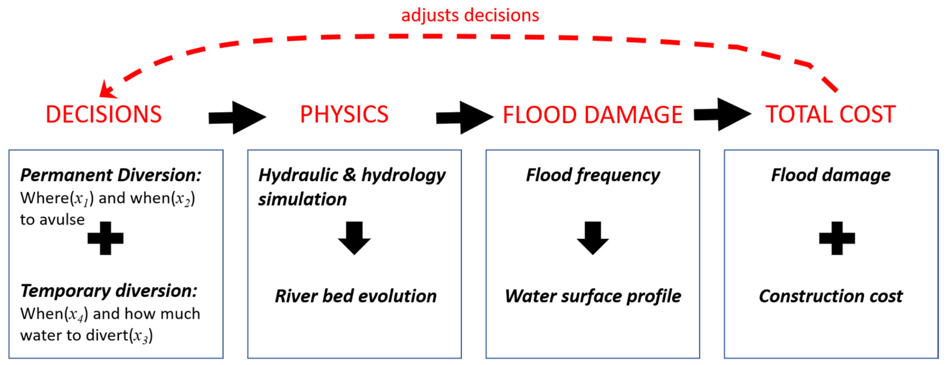
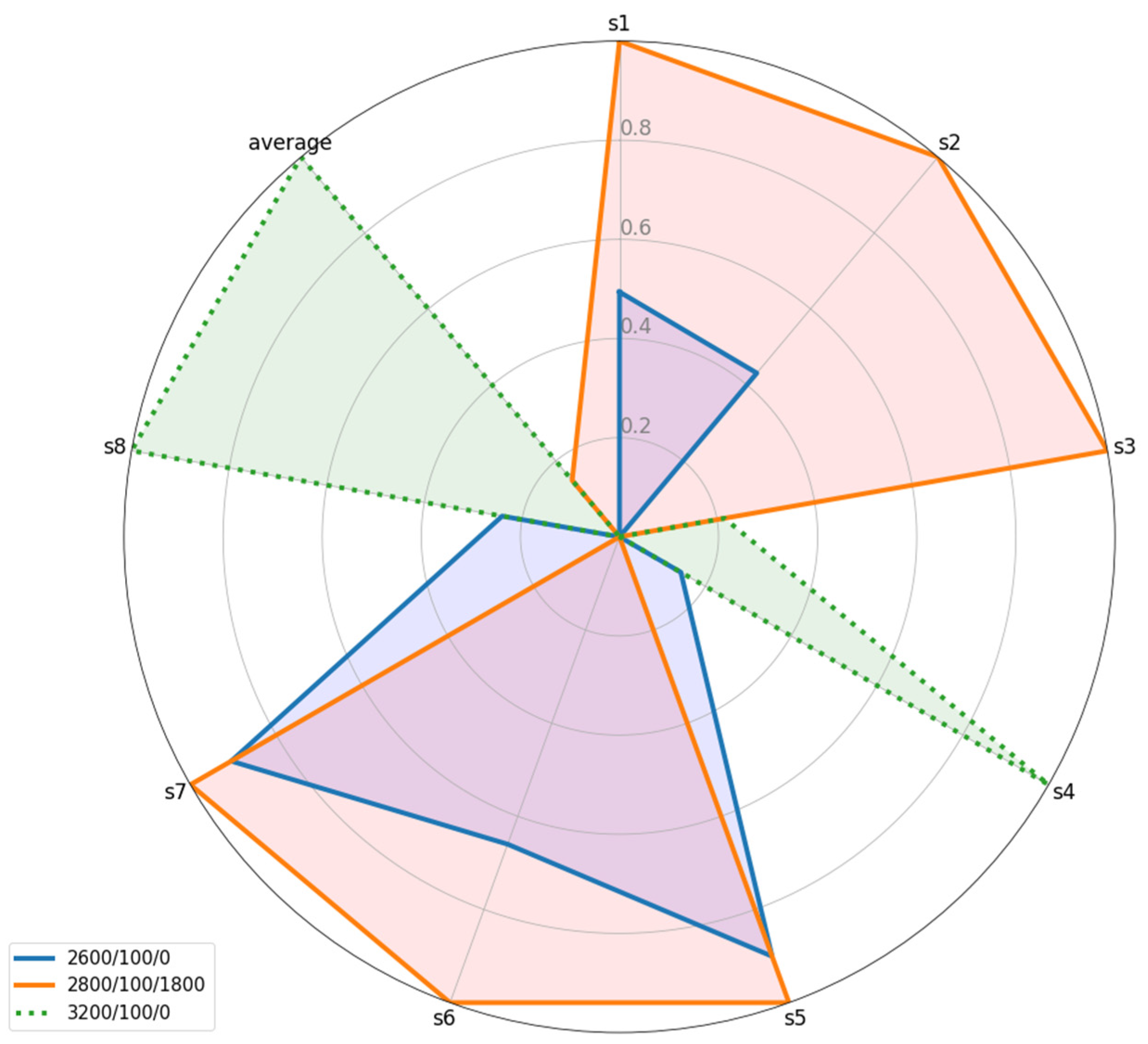
Table 1.
Summary of decision variables and their discrete values.
| Decision Variables | Definition | Considered Values | Unit |
|---|---|---|---|
| Avulsion rule | 2600, 2800, 3000, 3200, 3400 | ||
| Avulsion location | 70, 100 | ||
| Floodway size | 0, 900, 1800 | ||
| Floodway rule | 5000 |
Table 2.
Summary of all Year 2070 scenarios.
| Scenario | Mean Annual Flow | Mean Flood Flow | Sea Level Rise |
|---|---|---|---|
| S1 | Stay the same | Stay the same | 0.2 m |
| S2 | Stay the same | Stay the same | 0.5 m |
| S3 | Increase 20% | Stay the same | 0.2 m |
| S4 | Increase 20% | Stay the same | 0.5 m |
| S5 | Stay the same | Increase 20% | 0.2 m |
| S6 | Stay the same | Increase 20% | 0.5 m |
| S7 | Increase 20% | Increase 20% | 0.2 m |
| S8 | Increase 20% | Increase 20% | 0.5 m |
Table 3.
Summary of 250 alternatives in adaptive decision framework.
| Decision Variables | Stage | Considered Values | Number of Choices | Unit | ||
|---|---|---|---|---|---|---|
| First | 2600, 2800, 3000, 3200, 3400 | 25 | ||||
| Second | 2600, 2800, 3000, 3200, 3400 | |||||
| 70, 100 | 2 | |||||
| First | 0 | 900 | 1800 | 5 | ||
| Second | 0, 900, 1800 | 900 | 1800 | |||
| 5000 | 1 | |||||
Table 4.
Summary of the best and worst decisions and total cost under each scenario ( threshold triggering engineered avulsion decisions; location of engineered avulsion; floodway; river flow triggering the use of floodway).
Table 4.
Summary of the best and worst decisions and total cost under each scenario ( threshold triggering engineered avulsion decisions; location of engineered avulsion; floodway; river flow triggering the use of floodway).
| Decision Variable | Unit | S1 | S2 | S3 | S4 | ||||
| Best | Worst | Best | Worst | Best | Worst | Best | Worst | ||
| 3000 | 2800 | 3000 | 3400 | 2600 | 3400 | 2600 | 3400 | ||
| 100 | 70 | 100 | 70 | 70 | 100 | 70 | 100 | ||
| 0 | 1800 | 0 | 1800 | 0 | 0 | 0 | 0 | ||
| 5000 | 5000 | 5000 | 5000 | 5000 | 5000 | 5000 | 5000 | ||
| Total cost | million ¥ | 5138 | 5483 | 5210 | 5626 | 5404 | 6000 | 5733 | 6326 |
| Decision Variable | Unit | S5 | S6 | S7 | S8 | ||||
| Best | Worst | Best | Worst | Best | Worst | Best | Worst | ||
| 3200 | 2800 | 3000 | 3400 | 2600 | 3400 | 2600 | 3400 | ||
| 100 | 70 | 100 | 70 | 70 | 100 | 70 | 100 | ||
| 1800 | 1800 | 0 | 0 | 0 | 0 | 1800 | 0 | ||
| 5000 | 5000 | 5000 | 5000 | 5000 | 5000 | 5000 | 5000 | ||
| Total cost | million ¥ | 5615 | 6014 | 5734 | 6114 | 5925 | 6471 | 6239 | 6805 |
Table 5.
Summary of optimal second stage decision for each scenario, given first stage decision of { = 2600 , = 70 , 0 , = 5000 }.
Table 5.
Summary of optimal second stage decision for each scenario, given first stage decision of { = 2600 , = 70 , 0 , = 5000 }.
| Scenario | Optimal Second Stage Decision and Total Cost | ||
|---|---|---|---|
| Avulsion Rule | Floodway Capacity | Cost (million ¥) | |
| S1 | 2800 | 0 | 5195 |
| S2 | 3200 | 0 | 5369 |
| S3 | 2800 | 1800 | 5368 |
| S4 | 2600 | 1800 | 5712 |
| S5 | 2800 | 0 | 5733 |
| S6 | 3200 | 0 | 5902 |
| S7 | 3000 | 1800 | 5856 |
| S8 | 2600 | 1800 | 6190 |
Table 6.
Summary of expected cost (across scenarios) of open- and closed-loop decisions for each of the first stage decisions (Bold italicized red text indicates the optimal solution).
Table 6.
Summary of expected cost (across scenarios) of open- and closed-loop decisions for each of the first stage decisions (Bold italicized red text indicates the optimal solution).
| First Stage Decisions | Expected Costs (Million ¥) under Alternative Strategies, and Decrease in Cost Relative to Open Loop Strategy | ||||||||
|---|---|---|---|---|---|---|---|---|---|
| Closed Loop | Adaptive: Optimal Avulsion + Floodway | Δ | Adaptive: Optimal Avulsion Only | Δ | Adaptive: Optimal Floodway Only | Δ | |||
| 2600 | 70 | 0 | 5704 | 5665 | −39 | 5684 | −20 | 5687 | −17 |
| 2600 | 70 | 1800 | 5792 | 5761 | −31 | 5761 | −31 | 5792 | 0 |
| 2800 | 70 | 0 | 5799 | 5691 | −108 | 5713 | −86 | 5770 | −29 |
| 2800 | 70 | 1800 | 5870 | 5775 | −95 | 5775 | −95 | 5870 | 0 |
| 3000 | 70 | 0 | 5851 | 5803 | −49 | 5833 | −18 | 5815 | −36 |
| 3000 | 70 | 1800 | 5918 | 5898 | −19 | 5898 | −20 | 5918 | 0 |
| 3200 | 70 | 0 | 5810 | 5709 | −101 | 5720 | −90 | 5781 | −29 |
| 3200 | 70 | 1800 | 5821 | 5771 | −50 | 5771 | −50 | 5821 | 0 |
| 3400 | 70 | 0 | 5987 | 5741 | −245 | 5770 | −217 | 5875 | −112 |
| 3400 | 70 | 1800 | 5935 | 5795 | −140 | 5795 | −140 | 5935 | 0 |
| 2600 | 100 | 0 | 5834 | 5766 | −68 | 5798 | −36 | 5815 | −19 |
| 2600 | 100 | 1800 | 5895 | 5831 | −65 | 5831 | −64 | 5895 | 0 |
| 2800 | 100 | 0 | 5809 | 5773 | −36 | 5799 | −10 | 5782 | −27 |
| 2800 | 100 | 1800 | 5840 | 5832 | −8 | 5832 | −8 | 5840 | 0 |
| 3000 | 100 | 0 | 5775 | 5709 | −66 | 5731 | −44 | 5736 | −39 |
| 3000 | 100 | 1800 | 5795 | 5756 | −39 | 5756 | −39 | 5795 | 0 |
| 3200 | 100 | 0 | 5877 | 5720 | −156 | 5751 | −126 | 5840 | −37 |
| 3200 | 100 | 1800 | 5847 | 5738 | −109 | 5738 | −109 | 5847 | 0 |
| 3400 | 100 | 0 | 5970 | 5732 | −238 | 5770 | −200 | 5849 | −121 |
| 3400 | 100 | 1800 | 5890 | 5736 | −154 | 5736 | −154 | 5890 | 0 |
Table 7.
Sensitivity to cost assumptions of the expected benefit of allowing adaptive decisions (changes in and/or in second stage) for each of the first stage decisions (Bold red italics indicates optimal solution).
Table 7.
Sensitivity to cost assumptions of the expected benefit of allowing adaptive decisions (changes in and/or in second stage) for each of the first stage decisions (Bold red italics indicates optimal solution).
| First Stage Decisions | Increase Flood Damage Cost by 20% | Decrease Avulsion Construction Cost by 20% | Decrease Floodway Engineering Cost by 20% | ||||||||
|---|---|---|---|---|---|---|---|---|---|---|---|
| No Adapt. | Adaptive | Δ | No Adapt. | Adaptive | Δ | No Adapt. | Adaptive | Δ | |||
| 2600 | 70 | 0 | 6653 | 6529 | −124 | 5512 | 5458 | −54 | 5704 | 5604 | −100 |
| 2600 | 70 | 1800 | 6598 | 6545 | −53 | 5600 | 5553 | −47 | 5632 | 5601 | −31 |
| 2800 | 70 | 0 | 6739 | 6533 | −206 | 5580 | 5464 | −116 | 5799 | 5623 | −177 |
| 2800 | 70 | 1800 | 6664 | 6550 | −114 | 5650 | 5554 | −96 | 5710 | 5615 | −95 |
| 3000 | 70 | 0 | 6783 | 6660 | −123 | 5613 | 5565 | −48 | 5851 | 5742 | −110 |
| 3000 | 70 | 1800 | 6702 | 6670 | −33 | 5679 | 5650 | −29 | 5757 | 5738 | −19 |
| 3200 | 70 | 0 | 6705 | 6541 | −163 | 5543 | 5473 | −70 | 5810 | 5635 | −174 |
| 3200 | 70 | 1800 | 6558 | 6525 | −33 | 5554 | 5530 | −24 | 5661 | 5611 | −50 |
| 3400 | 70 | 0 | 6854 | 6553 | −302 | 5657 | 5477 | −180 | 5987 | 5678 | −309 |
| 3400 | 70 | 1800 | 6632 | 6515 | −117 | 5605 | 5515 | −90 | 5775 | 5635 | −140 |
| 2600 | 100 | 0 | 6776 | 6580 | −196 | 5609 | 5513 | −96 | 5834 | 5679 | −155 |
| 2600 | 100 | 1800 | 6689 | 6592 | −97 | 5670 | 5586 | −85 | 5735 | 5671 | −65 |
| 2800 | 100 | 0 | 6728 | 6590 | −139 | 5566 | 5520 | −46 | 5809 | 5687 | −122 |
| 2800 | 100 | 1800 | 6606 | 6593 | −13 | 5598 | 5587 | −11 | 5680 | 5672 | −8 |
| 3000 | 100 | 0 | 6673 | 6515 | −157 | 5518 | 5458 | −60 | 5775 | 5624 | −151 |
| 3000 | 100 | 1800 | 6537 | 6501 | −36 | 5538 | 5507 | −31 | 5635 | 5596 | −39 |
| 3200 | 100 | 0 | 6747 | 6496 | −251 | 5572 | 5443 | −129 | 5877 | 5629 | −248 |
| 3200 | 100 | 1800 | 6552 | 6458 | −94 | 5542 | 5469 | −73 | 5687 | 5577 | −109 |
| 3400 | 100 | 0 | 6828 | 6495 | −333 | 5634 | 5439 | −194 | 5970 | 5641 | −329 |
| 3400 | 100 | 1800 | 6571 | 6438 | −133 | 5553 | 5451 | −102 | 5730 | 5576 | −154 |
Table 8.
Summary of the best combination of first and second stage decisions under each scenario (deterministic analysis).
Table 8.
Summary of the best combination of first and second stage decisions under each scenario (deterministic analysis).
| Decision Variable | Unit | S1 | S2 | S3 | S4 | S5 | S6 | S7 | S8 | Average |
|---|---|---|---|---|---|---|---|---|---|---|
| 2600 | 3000 | 2600 | 3200 | 3400 | 3000 | 2600 | 3200 | |||
| 3400 | 2800 | 2800 | 2600 | 3400 | 2800 | 3000 | 2600 | |||
| 100 | 100 | 70 | 70 | 100 | 100 | 70 | 70 | |||
| 0 | 0 | 0 | 0 | 0 | 0 | 0 | 0 | |||
| 1800 | 0 | 1800 | 1800 | 1800 | 0 | 1800 | 1800 | |||
| 5000 | 5000 | 5000 | 5000 | 5000 | 5000 | 5000 | 5000 | |||
| Total cost | M¥ | 5114 | 5207 | 5368 | 5642 | 5585 | 5732 | 5856 | 6119 | 5578 |
| Improvement compared to no adaptation (Table 4) | M¥ | 24 | 3 | 36 | 91 | 30 | 2 | 69 | 120 | 47 |
Table 9.
Summary of value of information and value of flexibility (in million ¥).
| Solution and Cost | Non-Adaptive | Adaptive | Value of Flexibility: |
|---|---|---|---|
| 1. Perfect information | 5625 | 5578 | 47 |
| 2. Partial information | - | 5666 | |
| 3. No information | 5704 | 5704 | 0 |
| Value of perfect information: | 79 | 126 |
Table 10.
Comparisons of robust, adaptive decision vs. decisions under perfect information (in million ¥).
Table 10.
Comparisons of robust, adaptive decision vs. decisions under perfect information (in million ¥).
| Best 1st Stage Decision | E[Engineering Cost] | E[Flood Damage] | E[Total Cost] | |
|---|---|---|---|---|
| 1. Perfect information | 2600/70/No Floodway (most frequent) | 1464 | 4114 | 5578 |
| 2. Partial information | 2600/70/No Floodway | 960 | 4706 | 5666 |
| 3. No information | 2600/70/No Floodway | 907 | 4797 | 5704 |
Publisher’s Note: MDPI stays neutral with regard to jurisdictional claims in published maps and institutional affiliations. |
© 2021 by the authors. Licensee MDPI, Basel, Switzerland. This article is an open access article distributed under the terms and conditions of the Creative Commons Attribution (CC BY) license (https://creativecommons.org/licenses/by/4.0/).
Share and Cite
MDPI and ACS Style
Chen, L.; Hobbs, B.F. Robust Yellow River Delta Flood Management under Uncertainty. Water 2021, 13, 2226. https://doi.org/10.3390/w13162226
AMA Style
Chen L, Hobbs BF. Robust Yellow River Delta Flood Management under Uncertainty. Water. 2021; 13(16):2226. https://doi.org/10.3390/w13162226
Chicago/Turabian StyleChen, Liang, and Benjamin F. Hobbs. 2021. "Robust Yellow River Delta Flood Management under Uncertainty" Water 13, no. 16: 2226. https://doi.org/10.3390/w13162226
Note that from the first issue of 2016, this journal uses article numbers instead of page numbers. See further details here.