
Automated Detection of Instability-Inducing Channel Geometry Transitions in Saint-Venant Simulation of Large-Scale River Networks


1
Center for Water and the Environment, The University of Texas at Austin, Austin, TX 78758, USA
2
National Center for Infrastructure Modeling and Management, The University of Texas at Austin, Austin, TX 78758, USA
3
Oak Ridge National Laboratory, Oak Ridge, TN 37830, USA
*
Author to whom correspondence should be addressed.
Water 2021, 13(16), 2236; https://doi.org/10.3390/w13162236
Submission received: 2 June 2021
/
Revised: 28 July 2021
/
Accepted: 5 August 2021
/
Published: 17 August 2021
(This article belongs to the Section Hydraulics and Hydrodynamics)
Abstract
:A new sweep-search algorithm (SSA) is developed and tested to identify the channel geometry transitions responsible for numerical convergence failure in a Saint-Venant equation (SVE) simulation of a large-scale open-channel network. Numerical instabilities are known to occur at “sharp” transitions in discrete geometry, but the identification of problem locations has been a matter of modeler’s art and a roadblock to implementing large-scale SVE simulations. The new method implements techniques from graph theory applied to a steady-state 1D shallow-water equation solver to recursively examine the numerical stability of each flowpath through the channel network. The SSA is validated with a short river reach and tested by the simulation of ten complete river systems of the Texas–Gulf Coast region by using the extreme hydrological conditions recorded during hurricane Harvey. The SSA successfully identified the problematic channel sections in all tested river systems. Subsequent modification of the problem sections allowed stable solution by an unsteady SVE numerical solver. The new SSA approach permits automated and consistent identification of problem channel geometry in large open-channel network data sets, which is necessary to effectively apply the fully dynamic Saint-Venant equations to large-scale river networks or for city-wide stormwater networks.
1. Introduction
Solution of the full unsteady Saint-Venant equations (SVE) across large-scale open-channel networks has been shown to be computationally practical [1], but there remain a variety of roadblocks to effective and efficient applications for regional-to-continental scale river systems or city-wide stormwater networks. In particular, the SVE are prone to develop instabilities at sharp transitions due to the nonlinearities in the equations and interactions between fluxes, acceleration terms, and pressure gradients. Practitioners using SVE models (e.g., unsteady HEC-RAS [2]) are well-aware of such problems, typically using past experience and “engineering judgement” to smooth or remove troublesome geometry and obtain stable simulations. Such ad hoc fixes are readily applied in reach-scale hydraulic simulations where the location of the simulation instability and the appropriate fix can be diagnosed by simple visualization of results and trial-and-error geometry adjustments. However, our experience is that the ad hoc approaches become impractical over large-scale channel networks, which might consist of 10 to 10 reaches. When reaches are further subdivided to improve spatial resolution, a continental river dynamics model or the full SVE for a mega-city stormwater network could easily require 10 or more computational elements. For such systems we need automated methods to (i) identify locations and (ii) “fix” channel geometry that causes computational instabilities. Neither issue has been previously investigated in the literature. As this is the first study of numerical instabilities for large-scale flow networks simulated with implicit time-marching of the Saint-Venant equations, herein we focus solely on the issue of identifying troublesome geometry locations using an automated approach that is demonstrated at regional river network scales and is arguably practical at continental scales. The issue of automated approaches for fixing geometry problems is reserved as a subject for future research.
Motivating this work is our experience since Liu and Hodges [1] introduced the Simulation Program for River Networks (SPRNT). We have found that stable time-marching simulations are readily conducted using synthetic (prismatic) channel geometry, which can be generated using either hydrological characteristics or geographical features. However, the introduction of realistic geometry complexities with surveyed cross-section data tends to produce instabilities in the time-marching solution where sharp geometric transitions violate the underlying need for smoothness in numerical approximations of partial differential equations (see Yu et al. [3] for a discussion of non-smoothness effects of channel bottom slope). Unfortunately, the specific locations in a large network that cause an instability cannot be found simply from the convergence failure of the Newton solver in a nonlinear matrix solution. Such convergence failure is generally diagnosed by an norm that does not reduce or may increase with an instability. As a global measure, the norm cannot provide information on the specific locations of the problematic geometry. Furthermore, the behavior of the norm at non-convergence or behavior of the local error in the matrix cannot be used to identify the discrete locations causing instability—the iterative solution of a nonlinear matrix leads to the instability error being distributed throughout the of the system. If we wish to confine the future to the study of large networks with simplified prismatic cross-sections, then the state-of-the-art is satisfactory. However, with the availability of high-resolution bathymetry from recent advances in hyperspectral remote-sensing data and multi-beam sonar, we can expect future researchers and practitioners will introduce complex geometry into large-scale flow network simulations. There is a clear knowledge gap in how to efficiently analyze such networks to identify problematic geometry.
In our experience, the level of difficulty in identifying the geometry locations causing numerical instability in a Saint-Venant simulation will depend on both the overall scale of the network and the complexity of the geometry data. Unfortunately, trial-and-error methods that are easily applied in a single river reach become cumbersome in a large dendritic network with thousands of possible paths. The most obvious automated trial-and-error framework for a large network is applying independent “single-reach” simulations for all possible single-line paths through the flow network. Such an approach faces two key challenges: (i) identification of boundary conditions for each simulation, and (ii) comparative analyses of the set of simulations to identify locations of geometry problems. To address these issues, the approach to automated identification of problem geometry (as developed herein) uses successive simulations of a computationally-efficient steady-state SVE solver within a graph-theory method to isolate computational elements that cause numerical instabilities. The effectiveness of the approach is demonstrated with unsteady simulations of regional-scale river networks. This study builds on the steady-state SVE model of Yu et al. [4] developed from the unsteady SVE solver of Liu and Hodges [1]. Herein we propose a “sweep search algorithm" (SSA) that can systematically isolate any “choking points" in a large-scale open-channel network simulation. We use the characteristics of the dendritic river network and a simple traversal technique from graph theory for successive simulations with the steady-state SVE solver. The approach uses recursion to effectively examine the numerical convergence in every reach in the network. The information on convergence in the different branches provides automated identification of the locations of divergent behavior. The problem locations can be fixed by adjusting cross-section geometry. The SSA approach is demonstrated in two different open channel networks of and elements.
Background
For regional-to-continental scales, the transition from hydrological river models (i.e., reduced-physics such as [5,6]) to dynamic models (full SVE over all reaches, e.g., Liu and Hodges [1], Saleh et al. [7]) remains challenging, and the fundamental issues outlined in Hodges [8] have yet to be fully addressed. As noted therein, a key dynamic computational issue is that “problems at a single river cross-section can form a pinch point with numerical errors rapidly cascading through large sections of the network”. In city-wide stormwater modeling, variants of the US EPA Stormwater Management Model (SWMM) are often used, but the SVE—or “dynamic wave” approach—is recognized to have stability, convergence, and mass conservation issues [9]—which often causes users to switch to the reduced-physics kinematic wave option.
The transition from hydrologic network models to hydraulic network models has often been accompanied by the use simplified cross-sectional shapes [7,10,11,12], which are typically derived from hydrological characteristics such as cumulative drainage area or mean annual flow that change gradually through space [12,13,14,15,16]. Such approaches result in smooth geometry that is unlikely to cause instabilities and oscillations. However, as hydrologic data systems improve, modelers are gaining access to high-resolution data sets (e.g. Danielson and Gesch [17]) and river channel geometry databases [18] that are not artificially smoothed. Unfortunately, simple insertion of higher-resolution geometry into an existing, stable hydraulic model can lead to instabilities and oscillations due to sharp features in the high-resolution geometry.
The development and suppression of numerical instabilities and oscillations in SVE solvers have been widely discussed in the literature (e.g., Nujic [19], Garcia-Navarro and Vazquez-Cendon [20], Sanders [21], Tseng [22], Xing [23], Li et al. [24]) but there remains no simple, universal, or settled solution. Such problems can be triggered by (i) abrupt changes in lateral inflows [25,26], (ii) inconsistencies in initial conditions [4], (iii) non-Lipchitz source terms in the SVE formulation [3,27], and (iv) sharp transitions in the channel geometry. Herein, we focus only on the last issue.
Numerical oscillations/instabilities due to sharp changes in open-channel geometry can be provoked both by (i) changes in channel slope and (ii) changes in cross-sectional shape or area. The former issue is discussed and a solution provided in Yu et al. [3], where a “Reference Slope” is introduced to algebraically ensure the slope in the source term of an SVE model is a priori Lipschitz smooth. The latter issue, resolving sharp changes in flow area, does not seem amenable to a similar algebraic manipulation and hence is our focus herein. Such sharp transitions may be man-made (e.g., change in stormwater conduit size) or entirely natural. Arguably, the instabilities and oscillations developed by sharp transitions in open-channel cross-sectional shape could be addressed by creating an SVE solver that is unconditionally stable to any and all possible transitions. Such an algorithm cannot be proven unattainable, but it has been elusive thus far. Lacking a guaranteed approach for model stability, developers have investigated a wide variety of approaches to suppressing numerical instabilities. A popular approach is to suppress the non-linear properties (e.g., inertia terms) in the governing equation that typically cause instabilities in transitions across subcritical to supercritical flow [2,28,29]. Such ad hoc approaches can damp incipient instabilities, but they inherently undermine the simulation fidelity and limit the model applicability with trans-critical conditions.
For practitioners and researchers using a previously-developed model, issues of instability and oscillation are typically addressed when they can be seen in simulation results—with the challenge that an incipient numerical instability may only appear in some simulations at some combinations of flow rate and water surface elevation. Most model users do not have either the interest or time to delve into the numerical schemes that affect instabilities and modify the model source code. So the practical manual “fix” involves smoothing or replacing some channel geometry—typically with a trial-and-error approach—until a satisfactory convergent simulation is achieved [30]. This approach has two drawbacks: (i) the location causing the instability must be known, which can be problematic as a choke point causing a systematic network error might not be where the strongest oscillations or instabilities are observed, and (ii) such post hoc analysis and fixes are only effective until the next extreme event causes a new problem at a different location, requiring further manual adjustment. As we lack a cogent theory for a priori identifying problem geometry, what is needed (and is developed herein) is an efficient systematic approach to network analysis with the SVE that can be applied over a range of flow conditions. Our goal is a method that can be used to provide confidence that most, if not all, of the problem geometries have been identified across a wide range of likely flow conditions.
2. Methods
2.1. Governing Equations
The one-dimensional SVE, as proposed by de Saint-Venant [31], are the simplest equations that capture the momentum dynamics of a river reach. The momentum SVE is readily obtained by integrating the incompressible Navier-Stokes equations over a channel cross-section and applying the hydrostatic approximation. The SVE are widely used in both “conservative” [32,33] and “non-conservative” forms [34,35,36,37,38], although with non-uniform geometry this classic distinction becomes somewhat arbitrary, as discussed in Hodges [27]. In this study, we use the classic “non-conservative” form of the SVE from Liu and Hodges [1] in a finite-difference solution where the cross-sectional area (A) and flow-rate (Q) are primary solution variables of the numerical system. The local water depth (h) and friction slope () are derived variables that are expressed in function of A and Q. These SVE are written as
where is the local channel bottom slope and is the net lateral flow rate per unit length of the river, including inflows from the landscape and outflows to the groundwater aquifer. Variable h represents the local water depth and can be expressed by auxiliary function . The friction slope is computed by the Chezy-Manning equation, which can be written as
where is the representative Manning’s n roughness coefficient for the cross-section, and P is the wetted perimeter, which can be expressed as a function of A. Note that Yu et al. [3] have shown that without degrading the representation of geometric complexity, and h can be replaced by a smooth reference slope () and associated depth () with functions to ensure that the right-hand-side of Equation (2) does not include sharp transitions that are destabilizing. This new “Reference Slope” approach serves to isolate sharp geometry changes in the A and terms in the momentum equation. The new approach is recommended for practical large-scale SVE models, but is not used herein so that the results of the present work are entirely independent of Yu et al. [3].
As shown in Yu et al. [4], the steady-state solution of the SVE—which implies in Equation (1) is steady in time—can be easily solved for Q throughout a large network using a depth-first search (DFS) graph traversal technique (e.g., Cormen et al. [39]). The Q at any point in the “directed acyclic graph” (DAG) of the stream network is the sum of the upstream steady flows. With Q known everywhere, Equation (2) devolves into solving for the set of A, , and that implicitly satisfies:
Yu et al. [4] provides details of the Steady State Method (SSM) for solving this equation using a Preissmann discretization consistent with the SPRNT unsteady model of Hodges and Liu [40]. The SSM was shown to be superior to pseudo-time marching techniques that solve the unsteady SVE until convergence to a steady-state solution.
We use the SSM steady-state solver as a proxy for the unsteady SVE in analyzing the tendency of geometry to destabilize solutions in an open-channel network. Note that the SVE, Equation (2), and the SSM, Equation (4) have identical nonlinear advective terms, so it follows that failure of the steady-state solution to converge implies that the unsteady solution is also unlikely to converge.
2.2. Flowpath Topological Dependence
To quantify the internal heterogeneity of the river network and the topological overlap of flowpaths, we define the “flowpath topological dependence” () as a mathematical metric that represents the relationship of structural dependency between flowpaths. Topologically, river networks are Directed Acyclic Graph (DAG) systems because flow can never recirculate from downstream back to an upstream point. For simplicity herein, we will limit our focus to DAG systems that have single outlet and are dendritic trees, i.e., flow always accumulates in the downstream direction and distributaries (such as river deltas) are not allowed. Under these conditions, each streamhead has an unique flowpath to the outlet. Thus a river network system can be imagined as constructed of M flowpaths, with individual flowpaths designated as . Each is composed of a series of channel segments where and is thus the number of segments in . Flowpaths from different streamheads will overlap in downstream channels, as illustrated in Figure 1.
It is convenient to define as a matrix whose elements represent the fraction of the flow path that is shared with the flow path. Formally, this is
where is a sharing index for the v element of the i flowpath with all elements of the j flowpath, defined such that if channel segment v belongs to both flowpaths and if v is not in the j flowpath. The is asymmetrical in i and j as the v element of is not necessarily the v element of . Thus, .
To understand it is useful to consider two limiting cases. First, consider the sharing relationship of some flowpath, e.g., , with itself—this implies for the purposes of the sharing index in Equation (5). The result will be identically . Second, at the other limit is where two flowpaths, and , have no common segments (i.e., are in different networks) in which case provides the metric for commonality of the two paths. Between these limits we can imagine a flowpath of 10 segments that shares 5 of these segments with a flowpath of 20 segments. We find for this case that and , which can be thought of as 50% of is in common with , while only 25% of is in common with .
We use in the the Sweep Search Algorithm (below) to locate channel segments that likely are causing convergence problems.
2.3. Sweep Search Algorithm (SSA)
Our approach is to use a “Sweep Search Algorithm” for successive computations across each of the streamhead-to-outfall flowpaths () of the network. We can isolate the channel locations that cause convergence problems by analysis of the that fail to converge and the that share the same path and successfully converge. This is a form of “greedy” algorithm, which has consequences and limitations as noted in the Discussion, below.
In theory the SSA could be applied with the full unsteady SVE, but it would be extremely computational expensive to run the number of simulations required. Instead, we use the computationally efficient SSM steady-state solver of Yu et al. [4], as discussed in Governing Equations, above. A detailed workflow of the SSA is illustrated in Figure 2. There are three parts to this workflow: preprocess, iteration, and identification.
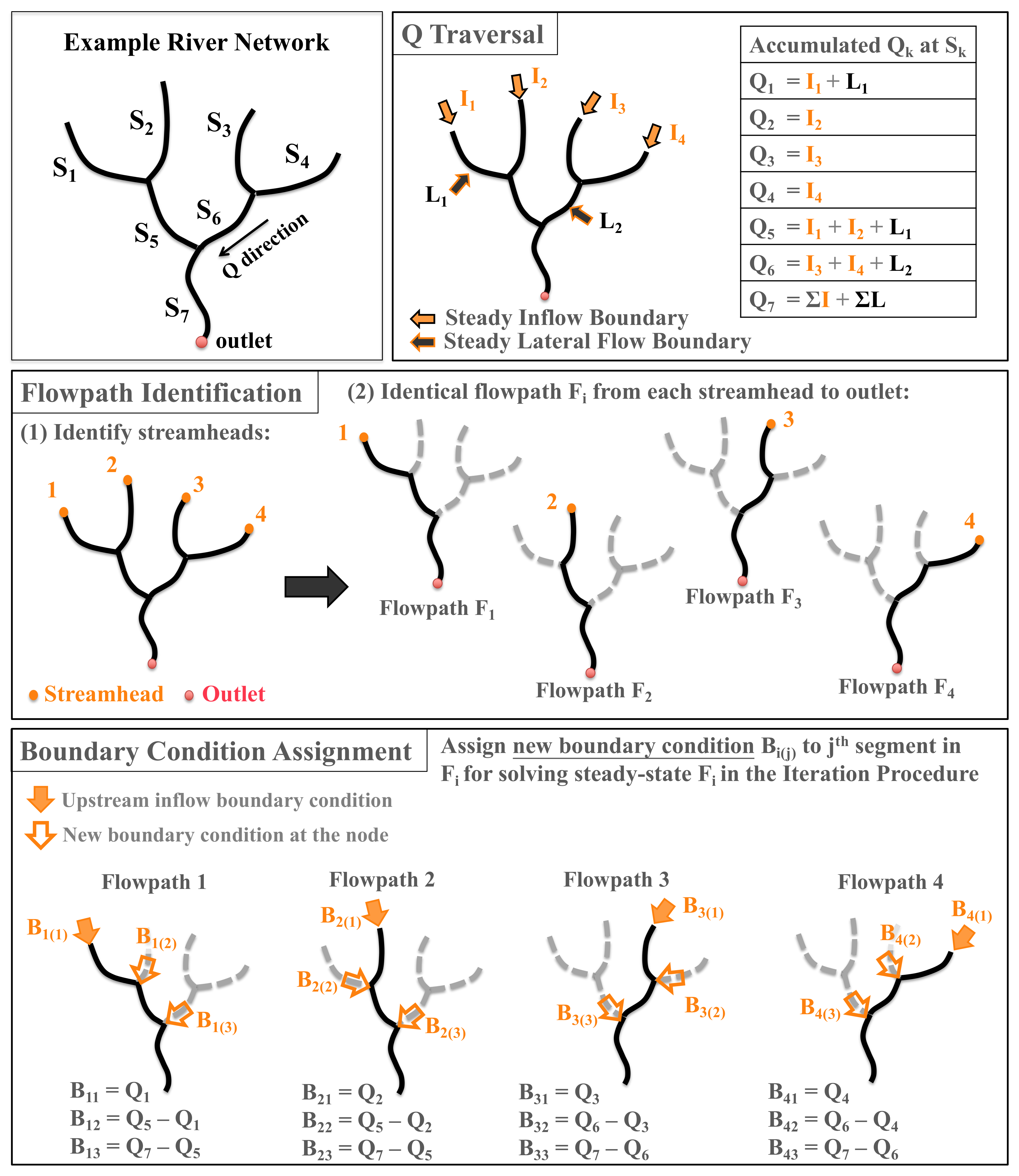
The Preprocess Procedure (PP) of the SSA method includes three steps: (I) Q traversal, (II) flowpath identification, and (III) boundary condition assignment. The Q traversal step takes the given steady-state hydrological flow boundary conditions (e.g., inflow boundary/lateral flow boundary) and uses the network topology to compute the corresponding flowrate () in the each of the k segments of the network, as outlined in Yu et al. [4]. The flowpath identification step identifies the v segments in the unique flowpath from each streamhead node to the river network outlet. In this nomenclature are the computational elements in the flowpath . Lastly, the boundary condition assignment step reassign the new boundary conditions to each identified flowpath base on the corresponding flowrate () computed from the Q traversal step. The new boundary condition is applied as node inflow to make sure the flow condition in each segment of the single flowpath is consistent with the in Q traversal step.
For steady flow, is simply the sum of the connected segments upstream of the k segment. The three steps of PP for an example river network with 7 reach segments are illustrated in Figure 3.
The SSA Iteration Procedure (IP) uses the steady solver (SSM) to recursively examine the numerical convergence of each flowpath in the river network. In this algorithm, the SSM solver is designed to start the examination from the flowpath with the most upstream streamhead, and sequentially proceed to downstream flowpaths. To satisfy the definition of the numerical convergence in this study, the Jacobian matrix’s L2 norm () between the Newton iteration steps in the SSM must be below , which is an arbitrary criteria set by the authors for model convergence. If the solver for the flowpath converges then the iteration moves on to the downstream flowpath, . If the SSM solver does not reach the converge criteria for the flowpath, the algorithm successively examines all other downstream flowpaths () with —i.e., all that share some part of the flowpath—until a converged is found. It is not unusual that multiple share the same value to . Flowpaths belong to one lateral limb can have the identical value to the main stem flowpath. For instance, and in Figure 3 are identical since and share the same overlap channel segment with . To delineate the priority of flowpaths with identical in the SSA iteration procedure, topological characteristic (in this study, flowpath length) is used as a ranking index for the SSM examination. The successive solutions begins with the flowpath where is a maximum for and . This corresponds to the flowpath with the most overlapped channel segments. When a converged is found, we can know that the geometry causing non-convergence is at the upstream section of the overlapped channel between and .
The third part of the SSA method—identification—provides an automated location of a problem segment, but it requires human intervention to fix the problem by adjusting the boundary conditions (channel reach geometry). The complexity of this procedure depends on the river structure and the resolution of input data. As noted in the Introduction Section above, our focus herein is on an automated approach for identifying the location of problematic river reaches, but fixing the underlying cause at any given section remains a matter of “art” that requires modeling judgement and, possibly, further trial-and-error iterations of the SSA method.
3. Computational Tests
3.1. Overview
The performance of SSA is examined with three different river network simulations with different scales. The scale of our test cases range from local-scale (with only two branches) up to a large scales that cover (i) a single river basin and (ii) the entirety of the Texas drainage basin (more than 35,000 stream segments). The number of computational nodes range from to in these three test cases. In the first test case, with a simple urban river topology, we demonstrate the SSA method by implanting an artificial sharp geometry transition at a channel section. The instability of the SSM solution along a flowpath with the new sharp transition and the convergence of flowpaths without the sharp transition provide proof-of-concept for the SSA screening method. In the large-scale test cases the SSA is applied to identify the problematic cross-section data in river networks with more complex topologies. In these tests, no artificial sharp features are introduced, we instead search for the expected discontinuities that typically occur in any large geometry data set. To show that the identified features are indeed the problem, we replace the cross-sections identified by the SSA with equivalent trapezoidal cross-sections and run both steady (SSM) and unsteady solvers to demonstrate convergence. The performance of the SSA is demonstrated and compared using both the required CPU time and number of Newton’s iterations for converged solution or onset of instability. All test cases are run on a Ubuntu Linux operating computer with 2.52 GHz Intel i7-870 CPUs with 16GB of RAM. The SSA algorithm and simulation codes are written in Python 2.7 and C++, with a shell script (bash) wrap-up.
3.2. Local-Scale Test Case—Waller Creek, Austin, Texas
A Y-shape urban river with high-resolution geometrical data in central Texas, Waller Creek, is selected in this study as a proof-of-concept test case for validating the SSA method. Following the “flowpath identification” in the preprocess procedure described in Methods and Figure 3, Waller Creek can be decomposed into two independent flowpaths: main stem () and minor branch () as shown in Figure 4. The 286 surveyed channel cross-sections (data courtesy of City of Austin) are used for the model geometry. Among the 286 cross-sections, 104 belong to the common channel section of and below the junction point (included in both flowpaths), whereas 33 and 149 are from the upstream branches of and (respectively) that occur in only one flowpath. The length of and flowpaths are 10.5 and 5.2 km, with total elevation difference 87.06 m and 44.09 m, respectively. The channel roughness coefficient (Manning’s n) of the computational elements in the two flowpaths ranges between 0.035 and 0.065. The bottom slope of Waller Creek with the closely-surveyed cross-sections includes sharp slope discontinuities, which herein are replaced with uniform slopes so that we focus on effects of sharp-transition channel geometry and exclude instabilities caused by a discontinuous bottom slope as these were treated in Yu et al. [3]. For the upstream reaches of and above the junction point, the are 0.0083 and 0.0116 respectively, whereas the overlapped downstream reach is set to 0.0071. The inflow boundary conditions are set to constant values of 50 m3/s and 30.63 m3/s at the upstream ends of and for steady-state Saint-Venant simulation in the iteration procedure of SSA method.
In this test case, we intentionally replace one cross-section in the upstream of the branch (only) by an artificial channel cross-section with a sharp geometry transition. This geometry simulates what might be either an unusual stream shape or an error in a data set. The artificial cross-section has a deep (2.39 m) narrow (1.06 m) channel with an approximately 19 m wide floodplain when water depth exceeds 2.3 m. The original and artificial cross-sections and the location in Waller Creek are illustrated in Figure 4. The sharp transition introduced between the very narrow incised channel and the flood plain are typical of features that we have seen cause numerical instabilities in a steady or unsteady solver. The SSM is used to simulate four different cases: (1) , (2) , (3) entirety of Waller Creek with original survey data (), and (4) entirety of Waller Creek with replaced geometry (). The numerical behavior and stability are analyzed in Results below.
3.3. River-Basin Test Case—Lavaca River, Texas
A single river basin for the Lavaca River, Texas (USA) provides the second test case. The dataset for this case is derived from Liu et al. [18] and uses the pre-defined rivers/streams structure from the National Hydrography Dataset Plus (NHDPlus). The Lavaca River network consists of 3049 km of river over a drainage area of 5971 km2. As first-order streams typically contribute little to network dynamics, herein we replace these in the data set with nodal inflows, which is similar to the approach of other researchers [41,42]. Removal of the first-order streams reduces the total channel length to 1291 km. The change of channel elevation in the NHDPlus data set is smooth and ranges between 0 m and 22.88 m above sea level. The maximum and minimum slope of the natural channel (excluding spillways and man-made hydraulic structures) are 0.0017 and 0.0001 respectively, with the average slope 0.0028. The mean annual flow at the outlet of the Lavaca River network is 30.84 m3/s. The total number of computation nodes in this model is 6973, with 6615 segments and 292 junctions. The spatial interval between the computational nodes ranges between 170 m to 200 m, with an average value of 183.3 m.
As we do not have a consistent surveyed dataset for channel geometry over the entire Lavaca River basin, we generate synthetic channel bathymetry following Zheng [43], which uses the height above nearest drainage (HAND) approach of Nobre et al. [44] applied to the National Elevation Dataset (NED). Although the HAND approximation is unlikely to be reasonable proxy of the in-channel river bathymetry, it serves the present purposes by providing a consistent and automated approach to generating non-prismatic cross-section from known topography. Our goal is not to provide an accurate topography model or test the validity of HAND, but to start from a model that we expect to have complex geometry with sharp transitions that affect model convergence. The data for channel roughness coefficient (Manning’s n) is acquired from the National Water Model (NWM) [45]. Values for Manning’s n from this source are between 0.05 and 0.06. Where the HAND data of Zheng [43] was incomplete, the missing channels were approximated as trapezoidal cross-sections using data from the NWM.
The necessary artificial inflow boundary conditions for steady-state solution are synthesized based on a uniform distribution of a typical downstream gauged flow over the headwater streams. That is, we take the flowrate at a USGS gauge 08164000 on 20 June 2018 (103.9 m3/s) and divide it by the 67 headwater streams to provide 1.55 m3/s inflow for each stream. Thus, for simplicity this test case has zero lateral inflows (i.e., zero local hydrological runoff) and distributes the actual measured downstream flow in uniform inflows over all the upstream branches. Clearly, this does not represent any real-world distribution of flows over the network, but it ensures that all branches of the network are activated and the total main-stream flow is representative of a real-world condition. This approach is useful in setting up test cases for geometry as it ensures that abrupt temporal changes in lateral inflows are not a confounding source of numerical instabilities. The slopes provided in the NHDPlus data for the Lavaca river network are known to be smooth (which is not true of every NHD network), so failure to converge a simulation for a flowpath in the Lavaca system is indicative of a problem with cross-section geometry.
3.4. Large-Scale Test Case—The Texas–Gulf Watershed
In order to demonstrate the SSA method over large networks, we apply it to the ten major river systems in the U.S. Hydrological Unit Code (HUC) Region 12—the Texas–Gulf Region—which contains 60,518 individual channel reaches with at total length of 184,798 km. As in the Lavaca River test case, we excluded 24,382 first-order streams in all river systems. Furthermore, the present approach has not been modified to handle channel distributaries; thus, 1104 minor streams having more than one downstream connection were excluded. The river topology and connectivity are derived from the divergence index in the NHDPlus dataset. The exclusion of minor streams results in the total number of reaches being 35,032 in the data set, with a total length of 90,693 km. The channel reaches are subdivided to 335,823 computational segments with 395,086 computational nodes. The average length of the computational segments is 192.54 m, with the range between 116.5 m and 200 m.
The channel elevation varies from 1364.4 m (upstream of Brazos River) to 0 m (sea level), with an average slope of 0.00283. Since the major scope of this study focuses on numerical instabilities from cross-sectional geometry transition, we performed smoothing on steep slopes greater than , which prevents instability-inducing slope discontinuities in of Equation (4). The smoothing reduces the overall average slope to 0.00272. As noted for the Waller Creek test case, the correct slopes can be used without generating instabilities through the Reference Slope method of Yu et al. [3], but the present work uses the smoothed slopes so that we isolate the effects of the new approach. The Manning’s n coefficients for all streams are retrieved from the National Water Model, ranging between 0.04 and 0.06.
Extending the approach in the Lavaca River test case, we used the HAND-generated bathymetry dataset created by Zheng [43] for the channel geometries across the entire HUC 12 region. The HAND dataset was filtered to exclude cross-sections deemed highly questionable based on our prior experience; these were cross sections characterized by (i) wetted areas that were not monotonically increasing with depth, (ii) incomplete cross-sectional bathymetry with less than 10 wetted area/depth data pairs, or (iii) inconsistent geometry—top widths less than 1 m combined with mean annual flow greater than 500 m3/s. This preliminary filtering was necessary because these highly questionable cross-sections can prevent the model from running, which is in contrast to more subtle geometry problems that result in numerical instabilities. This filtering affected 96 out of 34,504 reaches (0.27%). An additional 3116 reaches (11.6%) in our simulation did not have the corresponding HAND-generated channel geometries in the Zheng [43] dataset. Synthetic trapezoidal cross-sections as defined in the National Water Model [45] were used to fill the data gap.
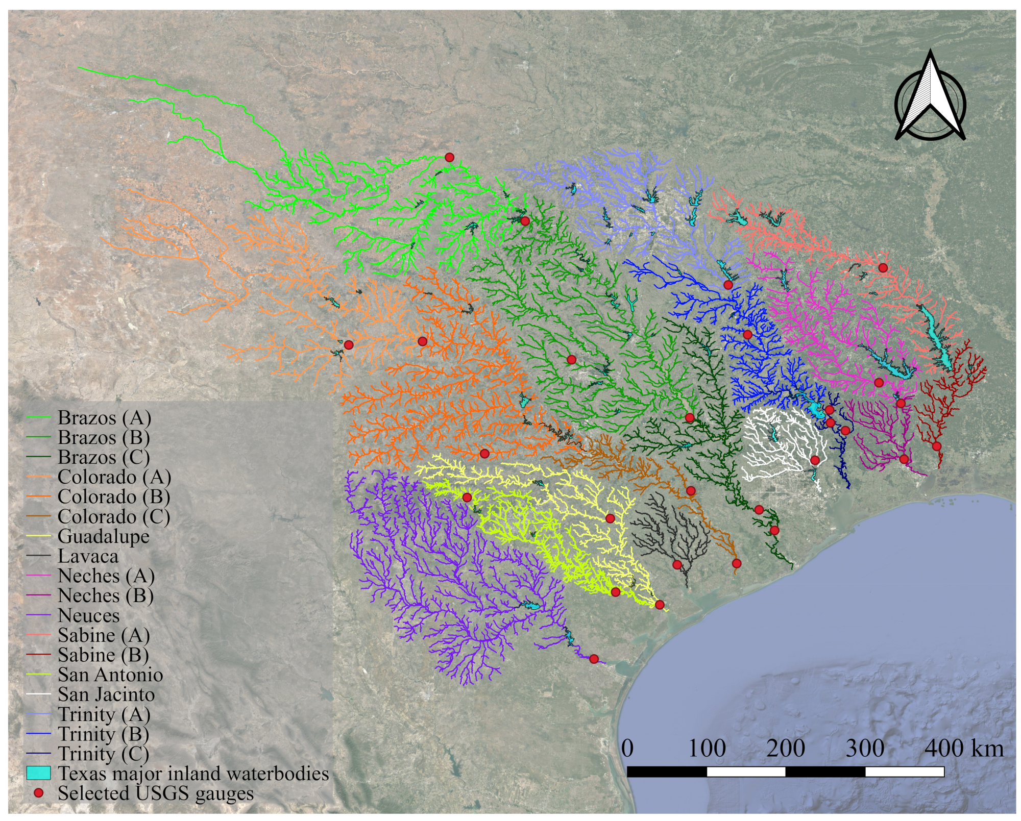
In theory, all the river basins could be handled by the SSA as a single data set since will be automatically defined where the i reach in one river system does not possess a common segment with the j reach in another system. However, it is convenient to divide the 10 river networks into 18 sub-networks for SSA analysis as illustrated in Figure 5. This subdivision serves two purposes: (1) allowing upstream inflow boundary conditions to effectively handle the steady-flow discontinuity implied by a reservoir, and (2) computational efficiency. The first issue is discussed in more detail below and the second issue is discussed in the Results Section. River network summary data are provided in Table 1.
The artificial inflow boundaries for this large-scale test case were developed from measured data by using 30 active USGS gauges in the 10 river systems across the Texas–Gulf basin shown in Figure 5. Since Texas rivers possess low flow during much of the year, the normal daily flowrates and mean annual flows will not necessarily result in geometry-induced instabilities. Thus, the flows generated on the most severe day of Hurricane Harvey, (daily measured maximum flowrates on 1 September 2017) were used for our steady-state test flow conditions. This approach ensures that the SSM solver is severely stressed.
The inflow boundaries use the same general approach as in the Lavaca River test case above; in other words, evenly dividing a downstream river system flowrate across all the associated upstream headwater reaches. However, USGS gauges in five of the river networks (Brazos, Colorado, Neches, Sabine, and Trinity) showed increasing reservoir storage during the time period. The steady-state SSM solver does not presently include the ability to handle unsteady storage, but the discontinuity at a reservoir is readily handled by breaking the larger river systems into smaller sub-systems, as illustrated in Figure 5. Thus, the river sub-network upstream of a reservoir used the reservoir inflow as the downstream flowrate for determining the headwater inflows, and the river sub-network downstream of a reservoir used the flow data from the reservoir outlet as an upstream inflow into the main stem. Using reservoir/dam as a natural internal boundary condition for connecting adjacent river networks is a common engineering practice in large-scale river modeling research [46]. Six out of eight subdividing points are selected based on active USGS gauges at/below the reservoir locations. Two additional subdividing points were identified at USGS gauges in the middle of the Brazos and Colorado river systems where significant discrepancies were noted between accumulated headwater inflow from the upstream network and the downstream gauge measurements. It is not uncommon to use the field survey gauge locations as the dividing points for river subdivision, as a similar idea was also employed in the NHDPlus HUC 4 watershed definition and delineation [47]. Details on how the gauge data were used to synthesize boundary conditions across all the river systems are provided in the Appendix A.
4. Results
4.1. Local-Scale Test Case—Waller Creek, Austin, Texas
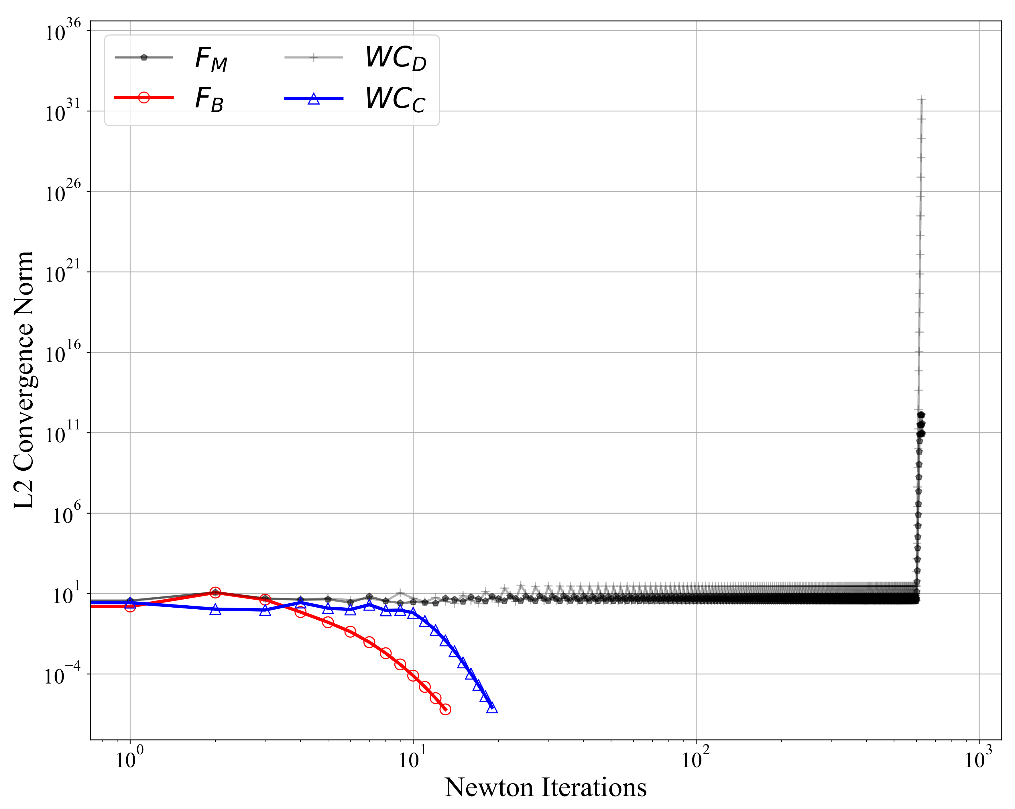
The numerical convergence behaviors for solving steady-state Saint-Venant equations by using geometries , , , and for the Waller Creek test case are shown in Figure 6. Unsurprisingly, the and cases (with the artificial sharp-transition geometry) failed to reach the convergence criteria (L2 norm <). In both cases, the convergence value in successive Newton iterations is initially relatively stable () but develops oscillatory behavior followed by a rapid climb near 600 iterations. This behavior indicates the presence of a discontinuity in the Jacobian matrix that cannot be converged by the solver.
By contrast, the and simulations (without the artificial sharp-transition geometry) rapidly reached converged solutions within 13 and 19 iterations, respectively. All four simulations were completed within 3 s of CPU time with a single computer core. What should be emphasized is the different fate of versus and , as shown in Figure 6. These results indicate that a single pinch point in the Saint-Venant simulation can result in catastrophic results in numerical stability of the whole simulation. Furthermore, the numerical stability of any flowpath containing the pinch point will be affected, which is the idea underlying the structure of the new SSA method.
The difference in CPU time between convergent/divergent simulations is trivial due to the simplicity of tested river network topology; however, a more significant difference can be expected in larger river networks with higher connectivity complexity as demonstrated in the following two cases.
4.2. River-Basin Test Case—Lavaca River, Texas
Without application of the new SSA method, the steady-state Saint-Venant simulation (SSM) for the Lavaca River network fails to converge under the flow conditions for 20 June 2018 (i.e., failed to reach the Newton iteration convergence criteria of an L2 norm ). This failure occurs despite the smooth bed slope of this river network and the use of ordinary (non-hurricane) flow conditions and uniform, steady, and upstream inflow conditions. Furthermore, without a viable initial steady solution, the unsteady solver cannot be converged [4]. Applying the SSA algorithm identifies a single channel segment as the problem. The location of the segment is illustrated in Figure 7. This segment caused failure of solutions for three flowpaths (red), while all other flowpaths (blue) were successfully solved in the SSA.
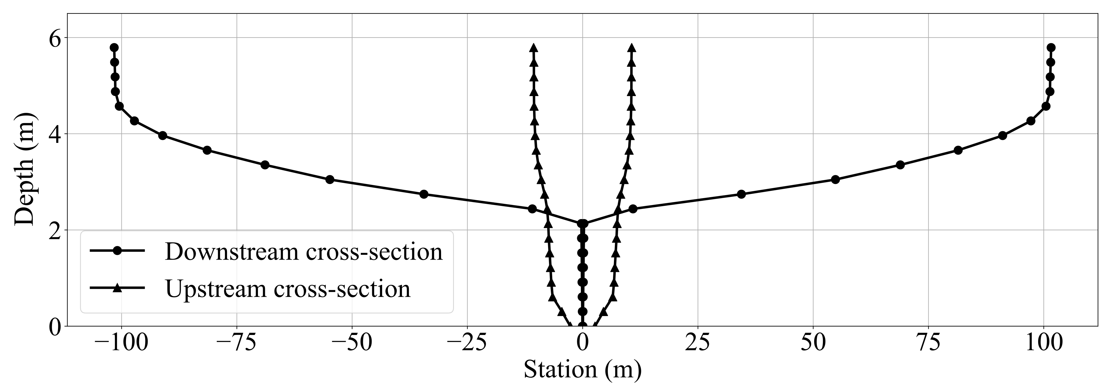
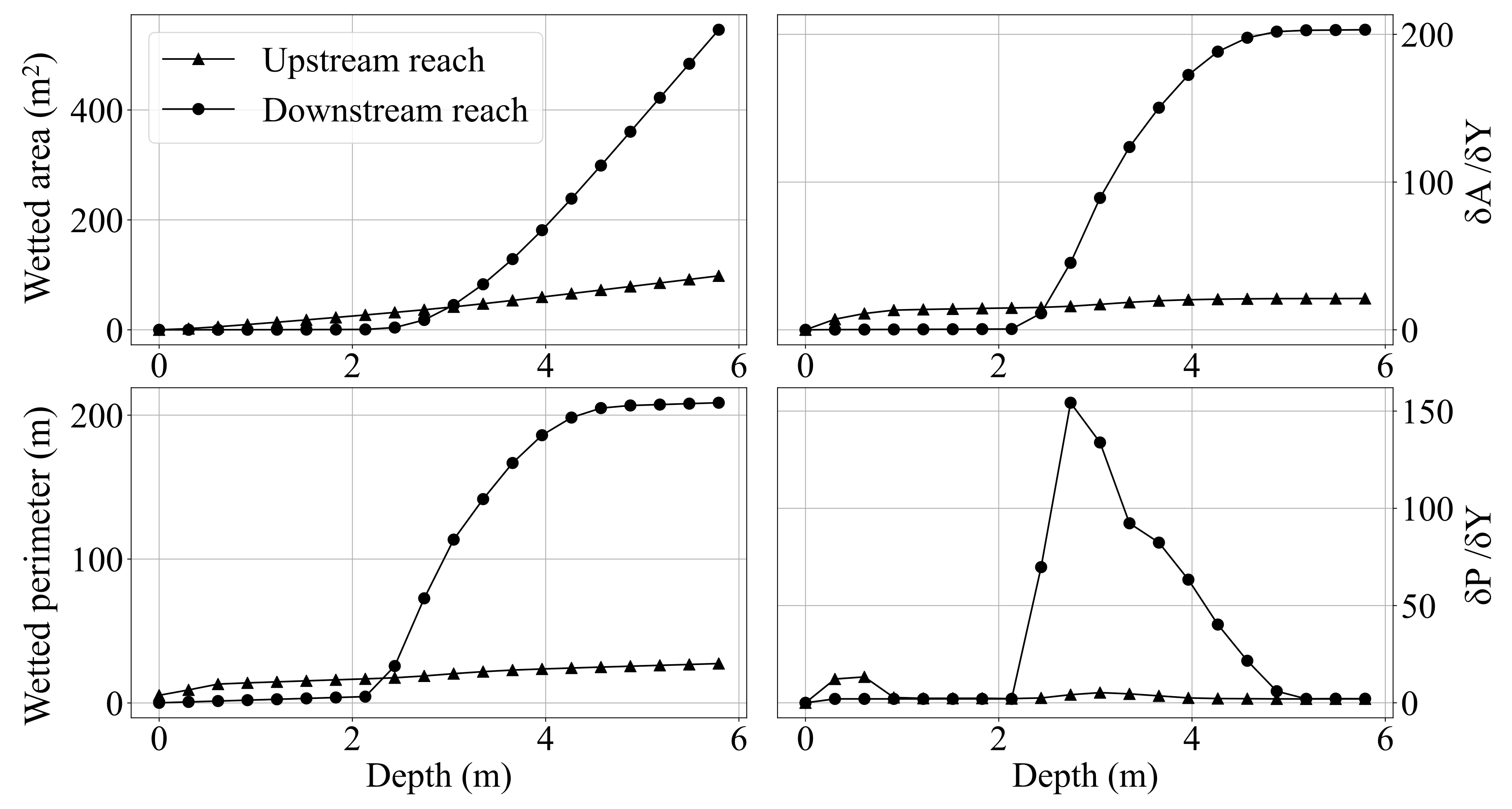
The problematic channel section for the Lavaca network is composed of two NHD flowlines, with mild local bed slopes ( and in the upstream and downstream respectively). Such mild slopes are unlikely to be the cause the convergence failure. The cross-sectional shapes of both NHD flowlines are illustrated in Figure 8. In addition, hydraulic geometry relationships of the two NHD flowlines are shown in Figure 9. It is clear that the upstream reach has smooth geometry across the full range of depths, whereas the channel width in the lower reach is extremely narrow ( m) below 2 m depth, and abruptly expands into a flood plain from 2–3 m depth. In other words, when water depth exceeds 2 m, the transition from the upstream to the downstream reach can create a sharp change in channel width between the cross-sections. The dramatic change of two adjacent geometrical boundary conditions can severely jeopardize the Lipschitz continuity of the discrete equations, required for a system to be differentiable and numerically stable [48]. From Equation (3) it follows that an sharp change in P with a smooth change in A for uniform Q and implies an sharp change in that is potentially destabilizing. As illustrated in Figure 9, the reaches the SSA identified as causing the instability show a sharp change in P from the upstream to downstream reach for water depths between 2 to 2.5 m. Thus, the failure of the SSM to converge with the given HAND geometry is consistent with theory for numerical instabilities.
A variety of approaches might be proposed for fixing these problem geometries, but such investigations are beyond the scope of the present work. Herein, the two problem HAND cross-sections (for all computational elements in the problem reach) were replaced with the trapezoidal cross-sections from the National Water Model, which is consistent with the way the HAND dataset of Zheng [43] was supplemented for missing data (see the Methods Section above). With these minor fixes, the original non-convergent SSM simulation of the entire Lavaca River network was readily converged.
The SSA method is fairly rapid, with overall CPU times for the Preprocess and Iteration steps of the SSA method applied to Lavaca River network shown in Table 2. Of course, these computational times are about two orders of magnitude smaller than the human intervention time required in the Identification procedure of the SSA for analyzing cross-sectional data and implementing an appropriate fix.
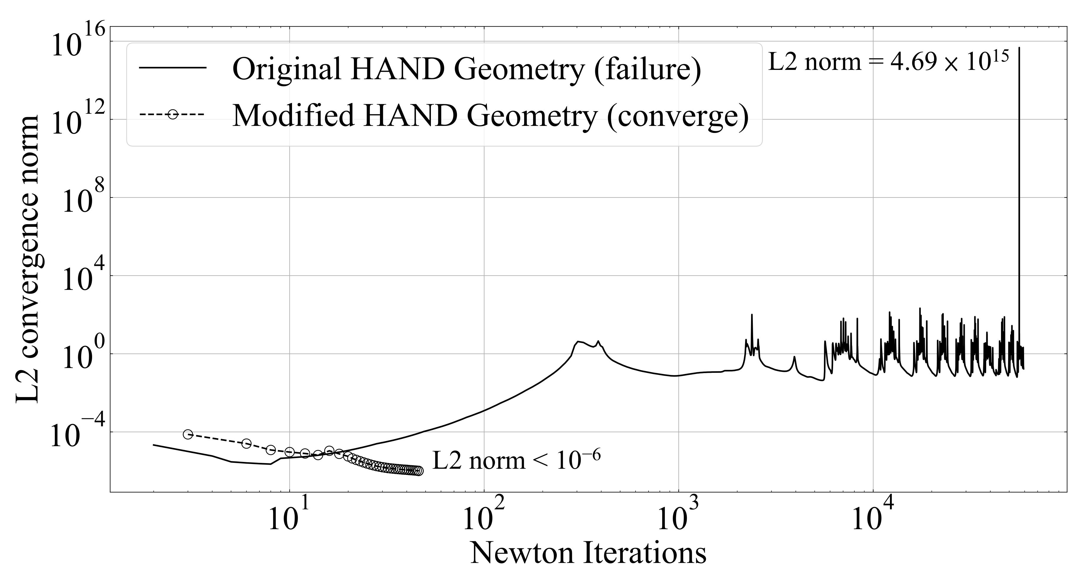
To visualize the effect that the change in the geometry of the one segment has on the solution of the entire Lavaca River network, Figure 10 shows the behavior of the convergence norm for the SSM solver before and after the geometry change. The L2 convergence norm for both simulations initially decreases and appears to be converging. However, the original geometry never reaches the convergence cutoff and begins to show oscillatory behavior that it cannot overcome. Indeed, if the SSM is allowed to run indefinitely using the original geometry an absurd spike of eventually appears in the L2 norm, indicating that solution has gone from oscillatory to unstable. Similar behaviors can also be found in the failure simulations in Waller Creek test case shown in Section 4.1. In contrast, the numerical solution of the modified geometry case smoothly reaches convergence after 46 iterations—less than 3 s of CPU time.
4.3. Large-Scale Test Case—Texas–Gulf Watershed
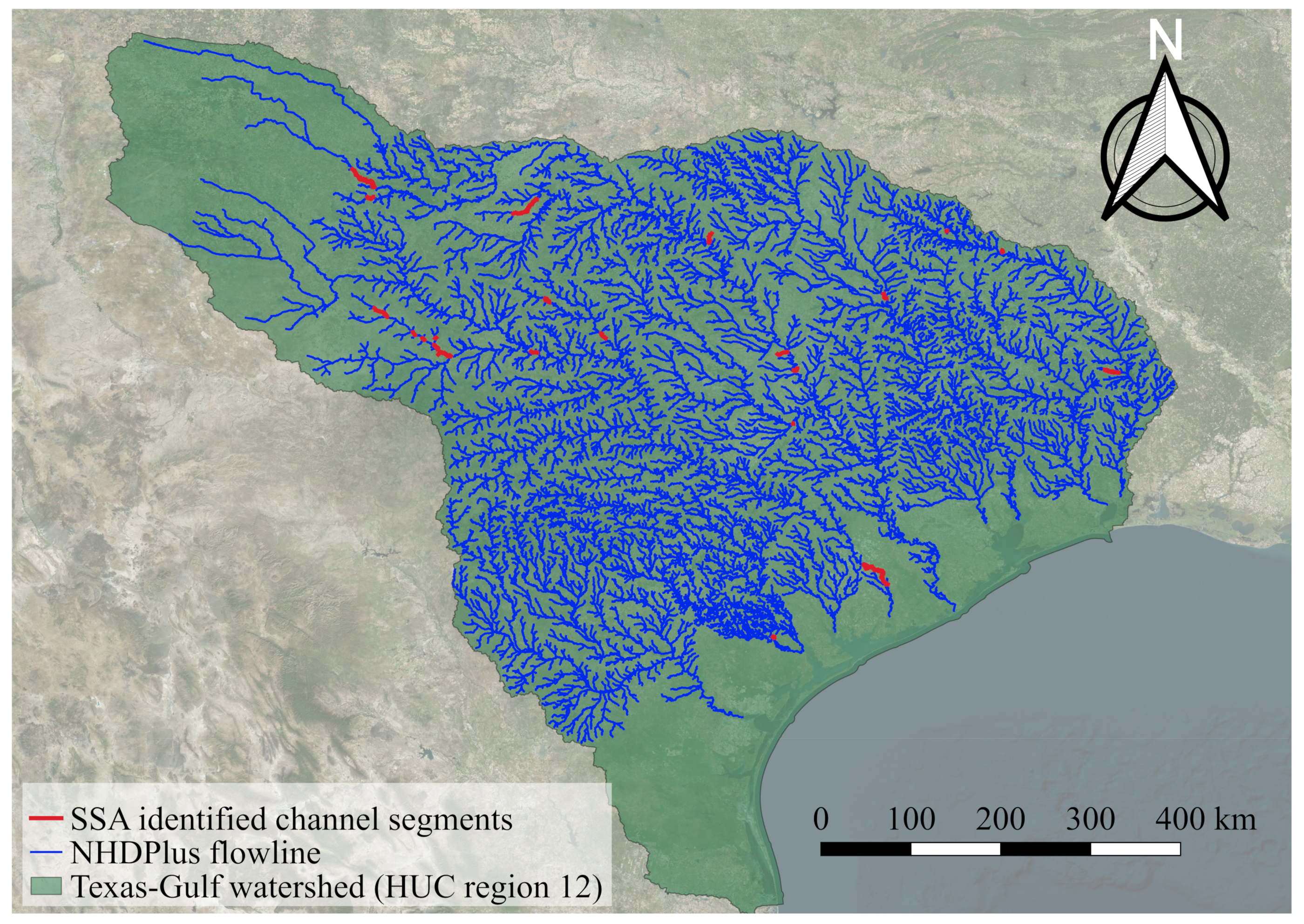
Among the eighteen river networks, seven of them failed to converge to a steady-state Saint-Venant solution under the test flow condition. The SSA method applied to the entire Texas–Gulf watershed identified convergence issues in 22 channel segments containing 153 NHDPlus flowlines. These problems occurred in seven subnetworks at the locations illustrated in Figure 11.
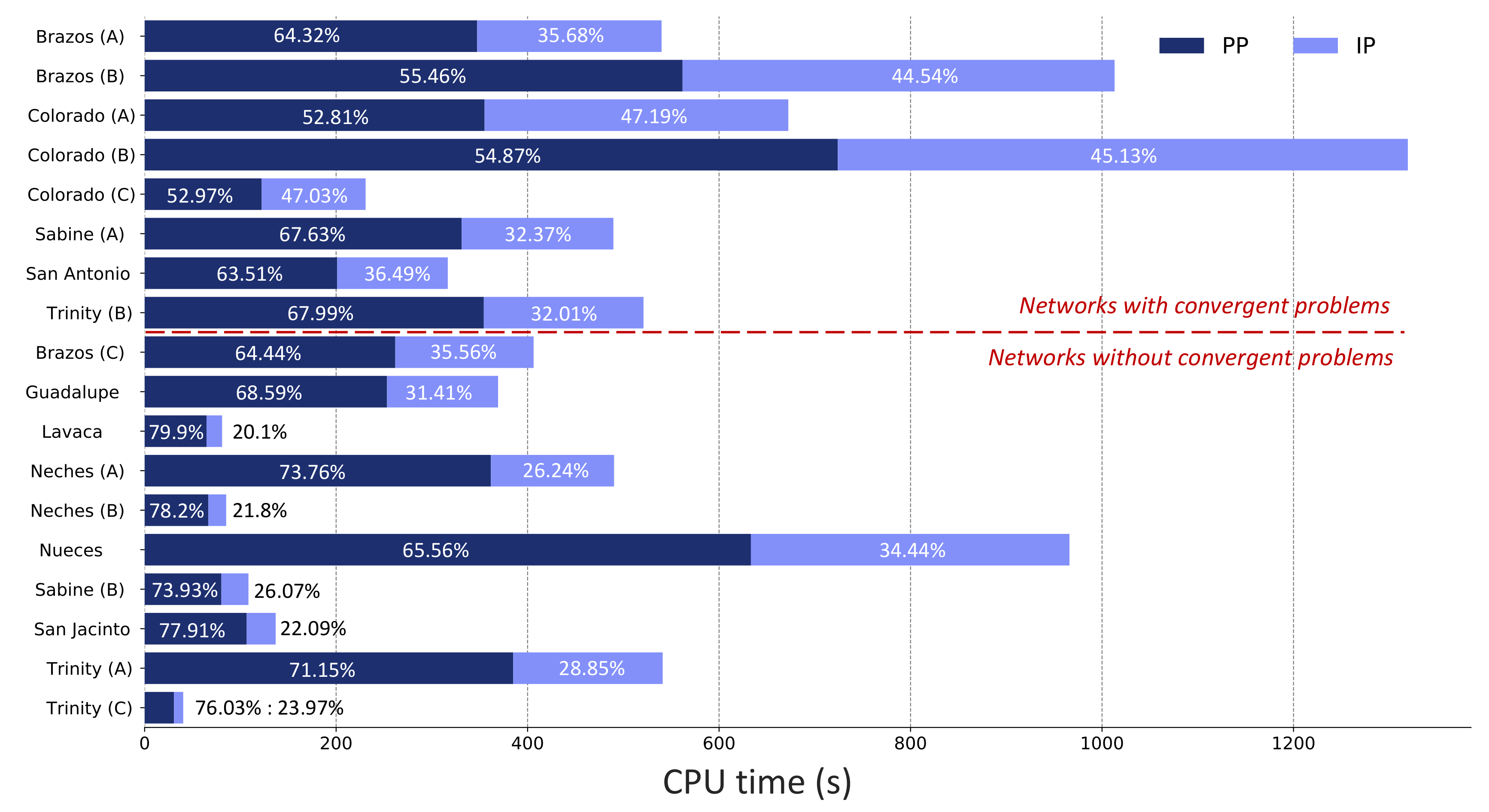
The total CPU time for the automated SSA algorithm (Preprocessing and Iteration, see Figure 3) for all 18 river networks are shown in Figure 12. Where no convergence problems occurred the iteration procedure using the SSM solver took roughly one-fourth of the computational time with the remainder being in the preprocessing procedure. When convergence problems were found the cost of iteration increased to one-third to one-half the overall computational time. Overall, running the SSA across the myriad of flowpaths for the entire Texas-Gulf watershed took less then 2-1/2 h on a modest desktop computer without any multi-threading optimization.
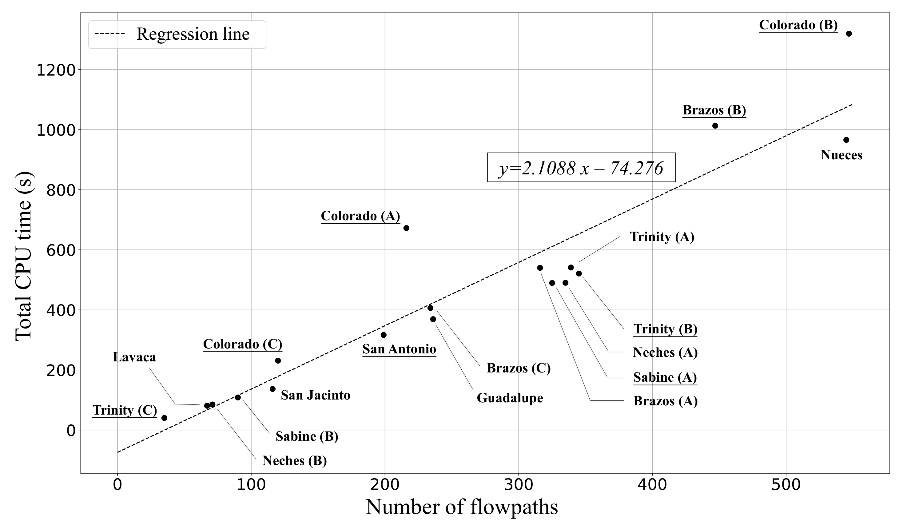
Despite what might be inferred from Figure 12, the presence or absence of convergence problems is not an important factor in the overall SSA CPU time. As shown Figure 13, the CPU time has a convincing linear regression () with the size of the system. That is, the number of flowpaths that must be preprocessed and iterated is the primary control on CPU time. Thus, the results in Figure 12 simply indicate that convergence problems are more likely to be found in larger systems with more flow paths.
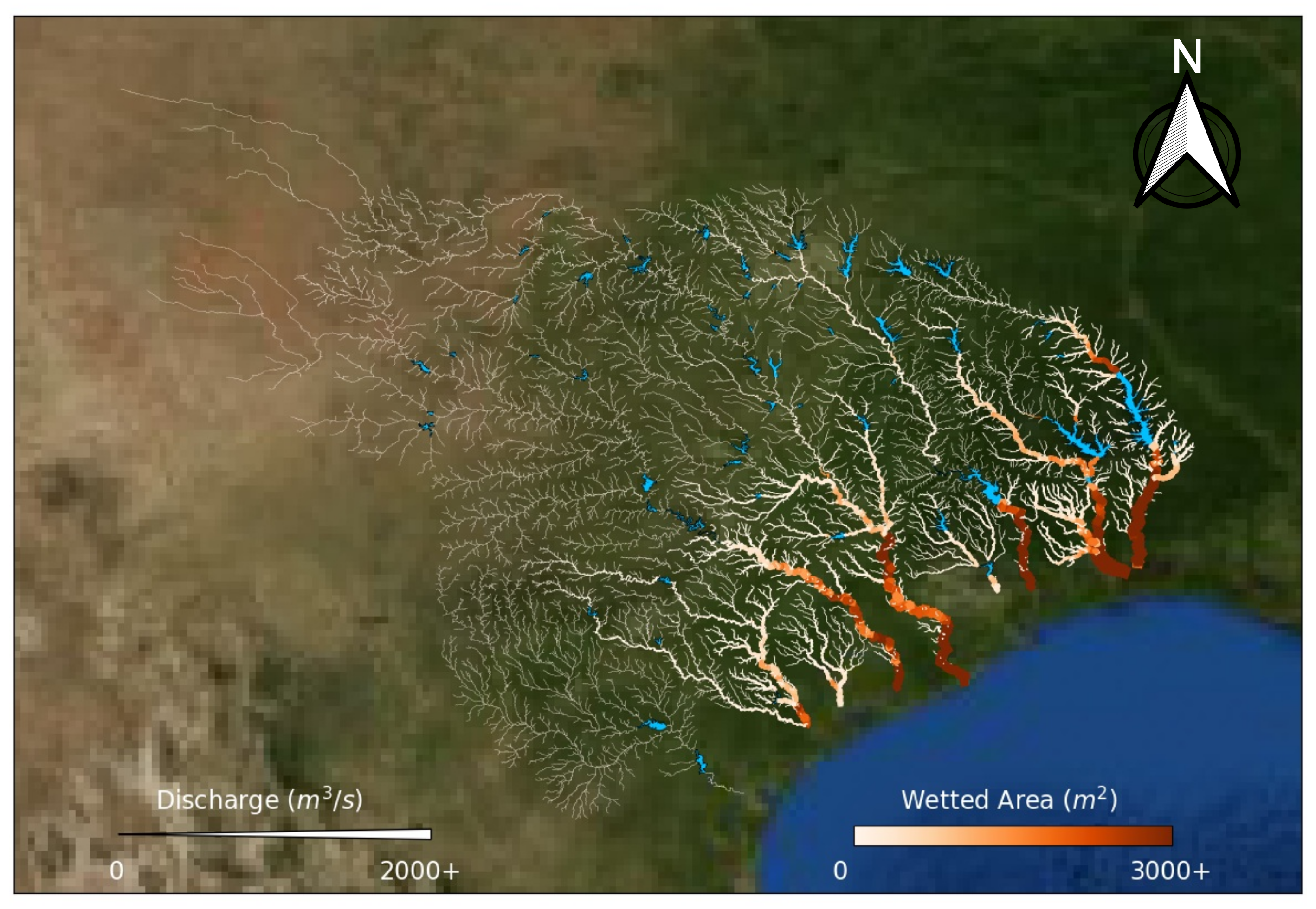
Among the 22 identified problem channel segments, 16 of them are located in the Brazos ((A), (B)) and Colorado ((A), (B)) river subnetworks. From the distribution shown in Figure 11, the majority are in streams with low Strahler stream orders (i.e., in the uplands of the network). Relatively few of the problem segments are in main stem or downstream channels. All the identified channel segments have hydraulic geometry issues with sharp transitions similar to those illustrated for the problem segment in the Lavaca River, above. Following the approach we used for fixing the problem segment in the Lavaca River, trapezoidal channel cross sections extracted from the National Water Model were inserted in place of the HAND geometry at each of the identified locations. With these changes, all 18 river networks successfully converged to stable steady-state solutions. The steady-state SVEs solution of all 26,842 NHDPlus flowlines on 1st September 2017 is illustrated in Figure 14.
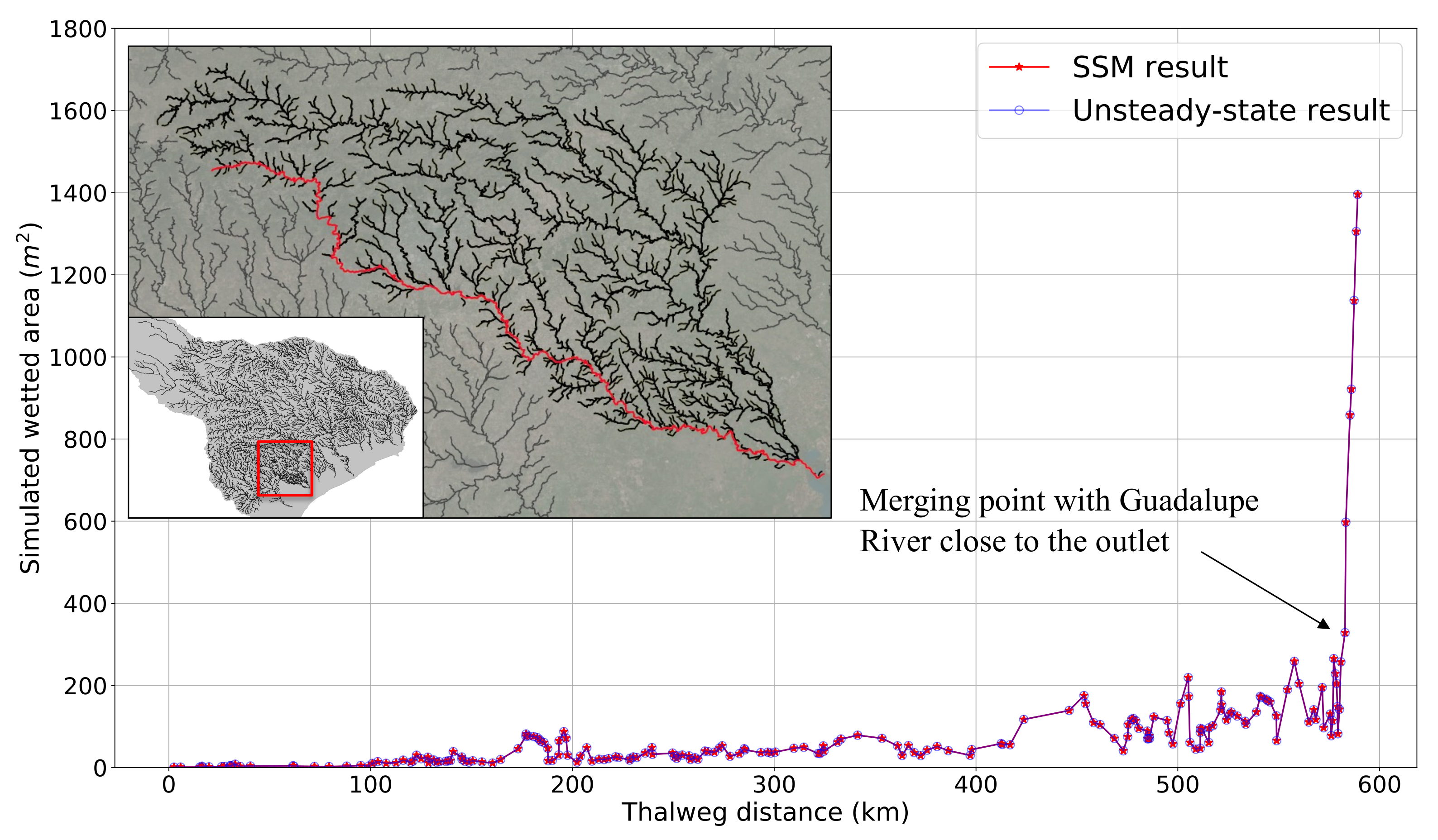
To demonstrate that the steady-state analysis approach of the SSA is a useful basis for unsteady modeling with the SVE, the steady solution in the main stem of San Antonio River (589.15 km) is compared with simulation results from the companion unsteady SVE solver [1] that is run until steady-state is achieved using identical inflow and lateral boundary conditions. The map of the selected channel and the simulated wetted area (A) from the two solvers are shown in Figure 15. The numerical results from the unsteady solver are practically identical to the solution with the SSM simulation for the steady boundary conditions—differences are of . This indicates the SSM reflects the underlying physics in the unsteady Saint-Venant equations with steady boundary conditions, which is our foundational idea for developing the SSA as a screening tool for the interaction of geometry and flow that leads to instabilities.
5. Discussion
Overall, the SSA/SSM approach is successful in efficiently diagnosing locations where interactions of geometry and steady flow cause non-convergence in a river network flow model. However, there are a number of issues that deserve discussion, including (i) inherent limitations of the method, (ii) limitations of the present implementation and testing, (iii) the use of HAND, (iv) improving computational time by parallelization, and (v) the need for automated approaches for fixing sharp transitions in geometry.
5.1. Inherent Limitations of SSA/SSM
The ability of the SSA/SSM method to diagnose locations that drive non-convergent behavior in a full unsteady Saint-Venant solver depends on the non-convergence being driven by the nonlinear advective term, the depth gradient term, or the source terms in Saint-Venant momentum (Equation (2)). That is, the SSA using the SSM cannot diagnose non-convergent behavior that is driven by unsteady phenomena—whether due to shocks in hydrological boundary conditions or shocks developed in unsteady flow. In theory, the SSA method could be extended to use an unsteady solver, but in practice the computational time would likely be prohibitive. Typically, an unsteady solver requires to more CPU time than an steady solver [4].
Despite this limitation, the SSA/SSM approach should be broadly successful because the interaction of the nonlinear advection term (in both steady and unsteady equations) with sharp geometry changes is typically the major source of the numerical instabilities. Indeed, this term is addressed for non-smooth topography by a range of authors [28,30,49,50,51]. Further, the nonlinear term is commonly suppressed in models (e.g., HEC–RAS, LIS–FLOOD) specifically to reduce oscillatory numerical behaviors [2,29]. Thus, the SSA/SSM provides a step forward as a quantitative framework to examine and fix the development of non-convergent solution behavior associated with sharp geometry changes.
A further limitation of the SSA method is that it requires the majority of the channel geometry must be reasonable and lead to convergent solutions. That is, if every possible flow path has non-convergent locations, the SSA method will not be able to isolate the precise stream reaches that cause problems. It seems likely that this limitation could be ameliorated by automated subdivision of networks to test flowpaths that are less than the full streamhead to river mouth, but investigation and demonstration of such an approach remains a subject for further investigation.
5.2. Limitations of the Present Implementation/Application
The present implementation of the SSA method is limited to strictly dendritic networks (no loops) with a single outlet. However, this is really a limitation of our implementation rather than the underlying concept. Loops and multiple outlets could be readily evaluated with the SSA method as long as the additional flowpaths, , associated with these topologies are defined. To keep our code simple we have not included these more complex configurations. Thus, our present code should be considered a proof-of-concept that needs further extension to cover more general river networks.
The present tests have been limited to the solution of a single set of extreme steady flow conditions for the Texas–Gulf watershed as a proof-of-concept exercise. However, in using the SSA as a precursor to full unsteady modeling, a wider range of steady-state conditions should be run to identify all the possible problem channels. It remains an open research task to understand what range of flow conditions should be tested to be confident that all possible instability-inducing geometries have been found.
5.3. Use of HAND-Generated Geometry
The present work appears to be the first large-scale application of HAND-generated geometry for the Saint-Venant solution of river basin networks. However, the suitability of using this proxy bathymetry dataset for SVE simulation remains an open question. Indeed, it is still unclear how the problematic sharp geometry changes arise in the computation of the HAND bathymetry and what this means for the physical reliability of HAND. Thus, our use of HAND herein should not be taken as an endorsement of the method for any particular application. It might be argued that such erroneous and abnormal channels are unlikely to occur with surveyed channel cross-sectional data and can be easily detected/fixed with simple screening functions. However, previous research has revealed that remote sensing data can systematically introduce uncertainties into the generated geometry of surface water-bodies [52,53]. Based on our experience and prior tests, these uncertainties cannot be easily ruled out in large scale river network and will further develop to instability factors in the simulation.
The reason for using HAND in our work simply because it is the only available comprehensive bathymetry data set. However, the SSA method could be similarly applied to any future comprehensive data set. Evaluating river network solutions using HAND against observed data and models applied with real cross-section bathymetry is a necessary exercise before HAND geometry can be taken as a accurate basis for modeling, but such efforts are beyond the present research scope. More details about the quality of the bathymetry generated by the HAND method can be found in Zheng et al. [54] and Godbout et al. [55].
5.4. Computational Time and Parallelization
As illustrated in Figure 13, the computational time has linear increase with the number of flowpaths that are screened with the SSA. Assuming the regression relationship holds, the required CPU time for the entire Mississippi River basin with 107,815 flowpaths in NHDplus would be approximately 63 h to test a single set of flow conditions. Thus, for large-scale applications there is a need to improve the operational speed of the code. As presented in Figure 2, the SSA algorithm is essentially serial. However, the Preprocess procedure (which takes most of the computational time) is likely parallelizable, and also can be duplicated as naive parallelization for different sets of flow conditions. Furthermore, the iteration procedure also seems amenable to parallelization. Each SSM solution is only a single flowpath and is entirely independent of every other flowpath. Hence, we could naively parallelize the iteration procedure across computer processors (i.e., without breaking up any single SSM solution) as long as the number of computer processors is less than the number of flowpaths. The identification and localization of non-convergent locations is then a comparison across a limited number of flowpath solutions. Furthermore, for finer parallelization a large dendritic network could be also parsed into subnetworks that could be independently parallelized—but the effectiveness of such an approach depends on whether a method can be created to synthesize internal boundary conditions at the subdivision points. Thus, we believe the SSA method could be readily extended to rapid solutions of continental river dynamics modeling using highly-parallel computers or GPU processors.
5.5. The Need for Automated Geometry Fixes
For the present work, all the identified problematic channel segments were manually examined and replaced with synthetic channel geometry from the NWM data set. We lack a general criterion for channel geometry replacement and/or adjustment, which is urgently needed to create a fully automated approach to fixing instability-inducing channel geometries. A variety of methods for generating synthetic channel geometry based on hydrological characteristics have been proposed [12,56,57], but there remains open questions as to the effects of introducing such synthetic geometry into a data set that is developed by other means (e.g., surveyed cross-sections, remote sensing). Note that sharp geometry problems might include both the local cross-section and its relationship to upstream and downstream cross-sections. Thus, there is a clear need for an automated approach to analyze local and neighbor cross-section geometry to make minimally-intrusive adjustments to reduce sharp transitions. An adequate theory for systematically analyzing river geometry contributions to non-convergence remains to be found and is the outstanding challenge to creating a fully automated approach for fixing sharp transitions.
6. Conclusions
In the pursuit of continental river dynamics modeling [8], we encounter increased fragility of numerical models as the complexity of the geometry and the size of the network are increased. As a practical matter, we can expect that any sufficiently large river network data set will contain either outliers or outright errors that cause model convergence issues. The SSA/SSM approach developed herein provides a framework for automated identification of problem locations—although effectively fixing the problem geometry remains a question of human intervention with some art and experience. As proof-of-concept we substitute trapezoidal cross-sections at problem locations, which is not a recommended long-term solution.
The SSA method uses a concept of Flowpath Topological Dependence to compare individual flowpaths whose solutions converge/diverge. The comparison of these paths allows isolation of the locations causing non-convergence. Herein, the SSA is tested in conjunction with SSM, a steady-state Saint-Venant solver [4] that can rapidly solve a single flowpath through a complex dendritic network. The SSA method is tested in a small proof-of-concept case with a local-scale urban river network and at full scale to examine the behavior of larger river systems covering the entire Texas-Gulf region (HUC region 12). We used HAND-generated geometry to provide a complete and consistent set of cross-section data over the entire network. Results showed that five of the river systems suffered from non-convergent solutions using extreme flow conditions. The SSA/SSM method effectively identified the 22 specific channel sections responsible for non-convergence in each network. The bathymetry in these sections all had sharp transitions with adjacent reaches. A simple “fix” using trapezoidal cross-sections from the National Water Model at these locations allowed both steady and unsteady Saint-Venant solvers to provide stable, converged solutions.
The overall computational costs of the SSA/SSM depends on both the river network topology and density of input data. In this study, 2.3 h of CPU time on a single computer core was required to analyze the 70,000 km of river reaches divided into 385,000 computational nodes over 10 river networks. The CPU time appears to increase linearly with the number of flowpaths, which indicates that the method must be extended with parallel computing and network partitioning techniques for use with continental-scale river networks.
This study shows the SSA/SSM method can identify the few locations in a large river network that cause convergence problems due to sharp geometry changes—a problem that is entirely impractical to investigate by hand or with unsteady river network simulations. The new method takes advantage of the computational speed-up obtained by recursively solving single flowpaths with a steady-state model, and provides a likely solution for troubleshooting nonconvergent hydrodynamic simulations in large-scale river network.
Author Contributions
C.-W.Y. designed the algorithm and performed the experiments. C.-W.Y. and B.R.H. analyzed the data and wrote the paper. F.L. wrote the code for the Saint-Venant solver in the Sweep Search Algorithm. All authors have read and agreed to the published version of the manuscript.
Funding
This work was partially supported by the U.S. National Science Foundation under grant number CCF-1331610 and the Cooperative Agreement No. 83595001 awarded by the U.S. Environmental Protection Agency to The University of Texas at Austin. This research has not been formally reviewed by EPA. The views expressed in this document are solely those of the authors and do not necessarily reflect those of the Agency. EPA does not endorse any products or commercial services mentioned in this publication.
Institutional Review Board Statement
Not applicable.
Informed Consent Statement
Not applicable.
Data Availability Statement
All tested data and scripts are uploaded to a public repository under Texas Data Repository [58] and can be accessed through https://doi.org/10.18738/T8/IPHYKM (accessed on 16 August 2021).
Acknowledgments
The authors would like to thank Xing Zheng for providing data for the test cases. The first author would like to thank Alan Plummer Associates Inc. for providing additional support during the latter stages of this project. The last author would like to acknowledge the support of the Laboratory Directed Research and Development Program of Oak Ridge National Laboratory, managed by UT-Battelle, LLC, for the US Department of Energy.
Conflicts of Interest
All authors declare no competing interest.
Notation
| A | Cross-sectional area () |
| g | Gravitational acceleration () |
| h | Water depth (m) |
| n | Manning’s roughness () |
| Flowpath topological dependence | |
| P | Wetted perimeter (m) |
| Q | Volumetric flow rate () |
| Flow rate per unit length through channel sides () | |
| Channel bottom slope | |
| Channel friction slope | |
| t | Time (s) |
| W | Channel width (m) |
| x | Along-channel spatial coordinate |
| Y | Certical height from channel bottom |
Appendix A. USGS Gauges of the Texas–Gulf Basin Selected for the Large-Scale Test Case
Due to the limited data availability, assumptions and estimations are made for the ungauged/remote streams and channels based on the nearby available measured hydrological information. In this study, a total number of 30 USGS gauges across the Texas–Gulf region are selected and served for different purposes. The information of the selected USGS gauges are listed in Table A1 with the gauge name, USGS code, drainage area, and the summary of the gauge data used in the simulation of each station. The selected USGS stations are used for three different purposes:
- Inflow boundary conditions determination. The measured flow data at the selected USGS stations are distributed uniformly across all the inflow boundaries at the streamhead reaches locate at the upstream of the selected gauge. This provides the synthetic inflow boundary at the streamheads of each channel.
- Downstream boundary condition determination. Measured water depth data at the selected USGS gauges are used to determine the downstream boundary conditions of each river network in the simulation. The selected USGS gauges are generally the gauges that are most downstream with available data in the river network.
- Internal boundary condition determination. Stations selected for determining internal boundary conditions are mostly located at reservoirs or along main stems with complete measured data. Internal boundary conditions are used to subdivide the river into multiple subnetworks. The measured water depth at the selected USGS gauge is then used to generate downstream boundary conditions for the upstream subnetwork, and the measured flowrate data are used as the inflow boundary condition for the downstream subnetwork. Using main stream gauges as breakpoints to split the river network is a common practice in hydrological routing in engineer applications (e.g., National Water Model flow nudging feature).

Table A1.
Information of selected USGS gauges in Texas–Gulf watershed.
| USGS Gauge Name | Station Code | River Name | Drainage Area | Hydrological |
|---|---|---|---|---|
| Information from the Gauge | ||||
| Cowhouse Creek at Pidcoke | 08101000 | Brazos River | 1178 | inflow boundary condition station |
| Brazos Rv nr Hempstead | 08115000 | Brazos River | 113,648 | inflow boundary condition station |
| Brazos Rv at Seymour | 08082500 | Brazos River | 40,243 | inflow boundary condition station |
| Brazos Rv at SH 21 nr Bryan | 08108700 | Brazos River | 101,136 | internal boundary condition and inflow boundary condition station |
| Brazos Rv nr Graford | 08088610 | Brazos River | 61,113 | internal boundary condition and inflow boundary condition station |
| Brazos Rv nr Rosharon | 08116650 | Brazos River | 117,427 | downstream boundary condition station |
| Pedernales Rv nr Fredericksburg | 08152900 | Colorado River | 955 | inflow boundary condition station |
| Colorado Rv nr Stacy | 08136700 | Colorado River | 62,659 | internal boundary condition and inflow boundary condition station |
| Colorado Rv at Austin | 08158000 | Colorado River | 101,032 | internal boundary condition and inflow boundary condition station |
| Colorado Rv nr Bay City | 08162500 | Colorado River | 109,401 | downstream boundary condition station |
| Concho Rv at San Angelo | 08136000 | Colorado River | 14,353 | inflow boundary condition station |
| Redgate Ck nr Columbus | 08160800 | Colorado River | 44.8 | inflow boundary condition station |
| Guadalupe Rv at Gonzales | 08173900 | Guadalupe River | 9039 | inflow boundary condition |
| Guadalupe Rv nr Tivoli | 08188800 | Guadalupe River | 26,231 | downstream boundary condition station |
| Lavaca Rv nr Edna | 08164000 | Lavaca River | 2116 | inflow boundary condition and downstream boundary condition station |
| Neches Rv nr Rockland | 08033500 | Neches River | 9417 | inflow boundary condition |
| Neches Rv nr Town Bluff | 08040600 | Neches River | 19,616 | internal boundary condition and inflow boundary condition station |
| Neches Rv Saltwater Barrier at Beaumont | 08041780 | Neches River | 25,353 | downstream boundary condition station |
| Nueces Rv at Calallen | 08211500 | Neuces River | 43,211 | downstream boundary condition station |
| Sabine Rv nr Beckville | 08022040 | Sabine River | 9295 | inflow boundary condition station |
| Sabine Rv at Toledo Bd Res nr Burkeville | 08025360 | Sabine River | 18,591 | internal boundary condition and inflow boundary condition station |
| Sabine Rv nr Ruliff | 08030500 | Sabine River | 24,162 | downstream boundary condition station |
| E Fork San Jacinto Rv nr New Caney | 08070200 | San Jacinto River | 1004 | inflow boundary condition and downstream boundary condition station |
| San Antonio Rv at Goliad | 08188500 | San Antonio River | 10,155 | downstream boundary condition station |
| Medina Rv at Bandera | 08178880 | San Antonio River | 849 | inflow boundary condition station |
| Upper Keechi Ck nr Oakwood | 08065200 | Trinity River | 388 | inflow boundary condition station |
| Trinity Rv at Trinidad | 08062700 | Trinity River | 22,113 | inflow boundary condition station and internal boundary condition |
| Menard Ck nr Rye | 08066300 | Trinity River | 393 | inflow boundary condition station |
| Long King Ck at Livingston | 08066200 | Trinity River | 365 | inflow boundary condition station |
| Trinity Rv nr Goodrich | 08066250 | Trinity River | 43,625 | internal boundary condition and inflow boundary condition station |
References
- Liu, F.; Hodges, B.R. Applying microprocessor analysis methods to river network modeling. Environ. Model. Softw. 2014, 52, 234–252. [Google Scholar] [CrossRef]
- Brunner, G.W. HEC-RAS, River Analysis System Reference Manual; U.S. Army Corps of Engineers, Hydrologic Engineering Center: Davis, CA, USA, 2016; p. 538.
- Yu, C.W.; Hodges, B.R.; Liu, F. A new form of the Saint-Venant equations for variable topography. Hydrol. Earth Syst. Sci. 2020, 24, 4001–4024. [Google Scholar] [CrossRef]
- Yu, C.W.; Liu, F.; Hodges, B.R. Consistent initial conditions for the Saint-Venant equations in river network modeling. Hydrol. Earth Syst. Sci. 2017, 21, 4959–4972. [Google Scholar] [CrossRef] [Green Version]
- Beighley, R.E.; Eggert, K.; Dunne, T.; He, Y.; Gummadi, V.; Verdin, K. Simulating hydrologic and hydraulic processes throughout the Amazon River Basin. Hydrol. Process. 2009, 23, 1221–1235. [Google Scholar] [CrossRef]
- Paiva, R.C.D.; Collischonn, W.; Tucci, C.E.M. Large scale hydrologic and hydrodynamic modeling using limited data and a GIS based approach. J. Hydrol. 2011, 406, 170–181. [Google Scholar] [CrossRef]
- Saleh, F.; Ducharne, A.; Flipo, N.; Oudin, L.; Ledoux, E. Impact of river bed morphology on discharge and water levels simulated by a 1D Saint–Venant hydraulic model at regional scale. J. Hydrol. 2013, 476, 169–177. [Google Scholar] [CrossRef]
- Hodges, B.R. Challenges in Continental River Dynamics. Environ. Model. Softw. 2013, 50, 16–20. [Google Scholar] [CrossRef]
- Rossman, L.A. Storm Water Management Model Reference Manual, Volume II—Hydraulics; Technical Report EPA/600/R-17/111; US EPA Office of Research and Development, Water Systems Division: Cincinnati, OH, USA, 2017.
- Strelkoff, T.; Clemmens, A. Approximating wetted perimeter in power-law cross section. J. Irrig. Drain. Eng. 2000, 126, 98–109. [Google Scholar] [CrossRef]
- Anwar, A.A.; de Vries, T.T. Hydraulically efficient power-law channels. J. Irrig. Drain. Eng. 2003, 129, 18–26. [Google Scholar] [CrossRef]
- Western, A.W.; Finlayson, B.L.; McMahon, T.A.; O’Neill, I.C. A method for characterising longitudinal irregularity in river channels. Geomorphology 1997, 21, 39–51. [Google Scholar] [CrossRef]
- Leopold, L.B.; Maddock, T. The Hydraulic Geometry of Stream Channels and Some Physiographic Implications; US Government Printing Office: Washington, DC, USA, 1953; Volume 252.
- Stall, J.B.; Fok, Y.S. Hydraulic Geometry of Illinois Streams; University of Illinois at Urbana-Champaign, Water Resources Center: Champaign, IL, USA, 1968. [Google Scholar]
- Singh, V.P.; Yang, C.T.; Deng, Z. Downstream hydraulic geometry relations: 1. Theoretical development. Water Resour. Res. 2003, 39. [Google Scholar] [CrossRef] [Green Version]
- Beighley, R.E.; Gummadi, V. Developing channel and floodplain dimensions with limited data: A case study in the Amazon Basin. Earth Surf. Process. Landforms 2011, 36, 1059–1071. [Google Scholar] [CrossRef]
- Danielson, J.J.; Gesch, D.B. Global Multi-Resolution Terrain Elevation Data 2010 (GMTED2010); Technical Report 2011-1073; US Geological Survey: Reston, VA, USA, 2011. [CrossRef]
- Liu, Y.Y.; Maidment, D.R.; Tarboton, D.G.; Zheng, X.; Wang, S. A CyberGIS integration and computation framework for high-resolution continental-scale flood inundation mapping. JAWRA J. Am. Water Resour. Assoc. 2018, 54, 770–784. [Google Scholar] [CrossRef] [Green Version]
- Nujic, M. Efficient implementation of nonoscillatory schemes for the computation of free-surface flows. J. Hydraul. Res. 1995, 33, 101–111. [Google Scholar] [CrossRef]
- Garcia-Navarro, P.; Vazquez-Cendon, M.E. On numerical treatment of the source terms in the shallow water equations. Comput. Fluids 2000, 29, 951–979. [Google Scholar] [CrossRef]
- Sanders, B.F. High-resolution and non-oscillatory solution of the St. Venant equations in non-rectangular and non-prismatic channels. J. Hydraul. Res. 2001, 39, 321–330. [Google Scholar] [CrossRef]
- Tseng, M.H. Improved treatment of source terms in TVD scheme for shallow water equations. Adv. Water Resour. 2004, 27, 617–629. [Google Scholar] [CrossRef]
- Xing, Y. Exactly well-balanced discontinuous Galerkin methods for the shallow water equations with moving water equilibrium. J. Comput. Phys. 2014, 257, 536–553. [Google Scholar] [CrossRef]
- Li, M.; Guyenne, P.; Li, F.; Xu, L. A positivity-preserving well-balanced central discontinuous Galerkin method for the nonlinear shallow water equations. J. Sci. Comput. 2017, 71, 994–1034. [Google Scholar] [CrossRef]
- Kvočka, D.; Falconer, R.A.; Bray, M. Appropriate model use for predicting elevations and inundation extent for extreme flood events. Nat. Hazards 2015, 79, 1791–1808. [Google Scholar] [CrossRef] [Green Version]
- Yang, L.; Hals, J.; Moan, T. Comparative study of bond graph models for hydraulic transmission lines with transient flow dynamics. J. Dyn. Syst., Meas. Control 2012, 134, 031005. [Google Scholar] [CrossRef]
- Hodges, B.R. Conservative finite-volume forms of the Saint-Venant equations for hydrology and urban drainage. Hydrol. Earth Syst. Sci. 2019, 23, 1281–1304. [Google Scholar] [CrossRef] [Green Version]
- Fread, D.; Jin, M.; Lewis, J.M. An LPI numerical implicit solution for unsteady mixed-flow simulation. N. Am. Water Environ. Congr. 1996, 96, 49–72. [Google Scholar]
- Bates, P.D.; Horritt, M.S.; Fewtrell, T.J. A simple inertial formulation of the shallow water equations for efficient two-dimensional flood inundation modelling. J. Hydrol. 2010, 387, 33–45. [Google Scholar] [CrossRef]
- Tayfur, G.; Kavvas, M.L.; Govindaraju, R.S.; Storm, D.E. Applicability of St. Venant equations for two-dimensional overland flows over rough infiltrating surfaces. J. Hydraul. Eng. 1993, 119, 51–63. [Google Scholar] [CrossRef]
- De Saint-Venant, A.B. Thé orie du mouvement non permanent des eaux, avec application aux crues des rivié res et à l’introduction des maré es dans leurs lits. Comptes Rendus Séances Acad. Sci. 1871, 73, 237–240. [Google Scholar]
- Catella, M.; Paris, E.; Solari, L. Conservative scheme for numerical modeling of flow in natural geometry. J. Hydraul. Eng. 2008, 134, 736–748. [Google Scholar] [CrossRef] [Green Version]
- Audusse, E.; Bristeau, M.; Decoene, A. Numerical simulations of 3D free surface flows by a multilayer Saint-Venant model. Int. J. Numer. Methods Fluids 2008, 56, 331–350. [Google Scholar] [CrossRef]
- Cunge, J. Evaluation problem of storm water routing mathematical models. Water Res. 1974, 8, 1083–1087. [Google Scholar] [CrossRef]
- Ponce, V.M.; Simons, D.B.; Li, R.M. Applicability of kinematic and diffusion models. J. Hydraul. Div. 1978, 104, 353–360. [Google Scholar] [CrossRef]
- Cunge, J.A.; Holly, F.M.; Verwey, A. Practical Aspects of Computational River Hydraulics; Pitman Publishing Ltd.: Boston, MA, USA, 1980. [Google Scholar]
- Abbott, M.; Bathurst, J.; Cunge, J.; O’connell, P.; Rasmussen, J. An introduction to the European Hydrological System—Systeme Hydrologique Europeen,“SHE”, 2: Structure of a physically-based, distributed modelling system. J. Hydrol. 1986, 87, 61–77. [Google Scholar] [CrossRef]
- Saleem, M.R.; Zia, S.; Ashraf, W.; Ali, I.; Qamar, S. The space–time CESE scheme for shallow water equations incorporating variable bottom topography and horizontal temperature gradients. Comput. Math. Appl. 2018, 75, 933–956. [Google Scholar] [CrossRef]
- Cormen, T.H.; Leiserson, C.E.; Rivest, R.L.; Stein, C. Introduction to Algorithms; MIT Press: Cambridge, MA, USA, 2009; Volume 2. [Google Scholar]
- Hodges, B.R.; Liu, F. Rivers and electrical networks: Crossing disciplines in modeling and simulation. Found. Trends Electron. Des. Autom. 2014, 8, 1–116. [Google Scholar] [CrossRef]
- Falter, D.; Dung, N.; Vorogushyn, S.; Schröter, K.; Hundecha, Y.; Kreibich, H.; Apel, H.; Theisselmann, F.; Merz, B. Continuous, large-scale simulation model for flood risk assessments: Proof-of-concept. J. Flood Risk Manag. 2016, 9, 3–21. [Google Scholar] [CrossRef]
- Paiva, R.C.D.; Collischonn, W.; Bonnet, M.P.; de Goncalves, L.G.G. On the sources of hydrological prediction uncertainty in the Amazon. Hydrol. Earth Syst. Sci. 2012, 16, 3127–3137. [Google Scholar] [CrossRef] [Green Version]
- Zheng, X. Texas River Hydraulic Properties. 2016. Available online: https://www.hydroshare.org/resource/40d4dfa1afb04cf9a64831c3419e7443/ (accessed on 24 April 2021).
- Nobre, A.; Cuartas, L.; Hodnett, M.; Rennó, C.; Rodrigues, G.; Silveira, A.; Waterloo, M.; Saleska, S. Height Above the Nearest Drainage—A hydrologically relevant new terrain model. J. Hydrol. 2011, 404, 13–29. [Google Scholar] [CrossRef] [Green Version]
- National Oceanic and Atmospheric Administration (NOAA). National Water Model (NWM); NOAA: Washington, DC, USA, 2016. [Google Scholar]
- Fleischmann, A.; Brêda, J.; Passaia, O.; Wongchuig, S.; Fan, F.; Paiva, R.; Marques, G.; Collischonn, W. Regional scale hydrodynamic modeling of the river-floodplain-reservoir continuum. J. Hydrol. 2021, 596, 126114. [Google Scholar] [CrossRef]
- Natural Resources Conservation Service (NRCS). Watersheds, Hydrologic Units, Hydrologic Unit Codes, Watershed Approach, and Rapid Watershed Assessments; USDA Natural Resources Conservation Service: Washington, DC, USA, 2007.
- Iserles, A. A First Course in the Numerical Analysis of Differential Equations; Cambridge University Press: Cambridge, UK, 1996; p. 378. [Google Scholar]
- Liggett, J.A.; Woolhiser, D.A. Difference Solutions of the Shallow-Water Equation; Cornell University Water Resources Center: Ithaca, NY, USA, 1967. [Google Scholar]
- Moussa, R.; Bocquillon, C. Criteria for the choice of flood-routing methods in natural channels. J. Hydrol. 1996, 186, 1–30. [Google Scholar] [CrossRef]
- Getirana, A.; Peters-Lidard, C.; Rodell, M.; Bates, P.D. Trade-off between cost and accuracy in large-scale surface water dynamic modeling. Water Resour. Res. 2017, 53, 4942–4955. [Google Scholar] [CrossRef] [Green Version]
- Durand, M.; Gleason, C.; Garambois, P.A.; Bjerklie, D.; Smith, L.; Roux, H.; Rodriguez, E.; Bates, P.D.; Pavelsky, T.M.; Monnier, J.; et al. An intercomparison of remote sensing river discharge estimation algorithms from measurements of river height, width, and slope. Water Resour. Res. 2016, 52, 4527–4549. [Google Scholar] [CrossRef] [Green Version]
- Pereira, B.; Medeiros, P.; Francke, T.; Ramalho, G.; Foerster, S.; De Araújo, J.C. Assessment of the geometry and volumes of small surface water reservoirs by remote sensing in a semi-arid region with high reservoir density. Hydrol. Sci. J. 2019, 64, 66–79. [Google Scholar] [CrossRef]
- Zheng, X.; Tarboton, D.G.; Maidment, D.R.; Liu, Y.Y.; Passalacqua, P. River channel geometry and rating curve estimation using height above the nearest drainage. J. Am. Water Resour. Assoc. 2018, 54, 785–806. [Google Scholar] [CrossRef]
- Godbout, L.; Zheng, J.Y.; Dey, S.; Eyelade, D.; Maidment, D.; Passalacqua, P. Error Assessment for Height Above the Nearest Drainage Inundation Mapping. JAWRA J. Am. Water Resour. Assoc. 2019, 55, 952–963. [Google Scholar] [CrossRef] [Green Version]
- Ferguson, R.I. Hydraulics and hydraulic geometry. Prog. Phys. Geogr. 1986, 10, 1–31. [Google Scholar] [CrossRef]
- Merigliano, M.F. Hydraulic geometry and stream channel behavior: A uncertain link. JAWRA J. Am. Water Resour. Assoc. 1997, 33, 1327–1336. [Google Scholar] [CrossRef]
- Yu, C.W.; Hodges, B.R.; Liu, F. Supporting Data for Automated Detection of Instability-Inducing Channel Geometry Transitions in Saint-Venant Simulation of Large-Scale River Networks. 2021. Available online: https://dataverse.tdl.org/dataset.xhtml?persistentId=doi:10.18738/T8/IPHYKM (accessed on 24 April 2021).
Figure 1.
Flowpaths from two streamheads with unique (red and green) and overlapping (black) channels. Stream channels include the Upper Onion Creek, Texas, USA.
Figure 1.
Flowpaths from two streamheads with unique (red and green) and overlapping (black) channels. Stream channels include the Upper Onion Creek, Texas, USA.

Figure 2.
Flowchart of the SSA method.

Figure 3.
The three steps in the preprocess procedure: Q traversal, flowpath identification, and boundary condition assignment steps are illustrated with an example river network with 7 channel segments.
Figure 3.
The three steps in the preprocess procedure: Q traversal, flowpath identification, and boundary condition assignment steps are illustrated with an example river network with 7 channel segments.

Figure 4.
In the preprocess procedure of SSA method, Waller Creek is decomposed to two flowpaths, and . The corresponding channel geometries of each flowpath are also shown (river geometry survey data courtesy of the City of Austin).
Figure 4.
In the preprocess procedure of SSA method, Waller Creek is decomposed to two flowpaths, and . The corresponding channel geometries of each flowpath are also shown (river geometry survey data courtesy of the City of Austin).

Figure 5.
Spatial distribution of 18 subdivided networks from 10 major river systems in Texas–Gulf region. The 30 selected USGS gauges for determining the flow condition in the test case are also shown.
Figure 5.
Spatial distribution of 18 subdivided networks from 10 major river systems in Texas–Gulf region. The 30 selected USGS gauges for determining the flow condition in the test case are also shown.

Figure 6.
Comparison of convergence for Waller Creek test case with () and without () an artificial sharp-transition cross-section that causes instabilities.
Figure 6.
Comparison of convergence for Waller Creek test case with () and without () an artificial sharp-transition cross-section that causes instabilities.

Figure 7.
The map of the Lavaca River network and the problematic channel segment identified by the SSA method.
Figure 7.
The map of the Lavaca River network and the problematic channel segment identified by the SSA method.

Figure 8.
Cross-sectional geometries of the problematic adjacent channel segments highlighted in Figure 7.
Figure 8.
Cross-sectional geometries of the problematic adjacent channel segments highlighted in Figure 7.

Figure 9.
Hydraulic properties of the adjacent channel geometries for the problem reach of the Lavaca network test case. Gradients and represent the changes in channel cross-sectional areas (A) and wetted perimeter (P) as a function of local depth (Y) in the upstream and downstream reaches.
Figure 9.
Hydraulic properties of the adjacent channel geometries for the problem reach of the Lavaca network test case. Gradients and represent the changes in channel cross-sectional areas (A) and wetted perimeter (P) as a function of local depth (Y) in the upstream and downstream reaches.

Figure 10.
Comparison of the L2 norm for Newton iterations in the Lavaca River network simulation with SSM solver. The simulation with original geometry is shown in the star plot, and the modified geometry is shown in circle plot.
Figure 10.
Comparison of the L2 norm for Newton iterations in the Lavaca River network simulation with SSM solver. The simulation with original geometry is shown in the star plot, and the modified geometry is shown in circle plot.

Figure 11.
SSA method identified NHD flowlines with instability factors in bathymetry.

Figure 12.
CPU time for executing the SSA algorithm in 18 river networks in the Texas–Gulf region. PP indicates SSA Preprocessor Procedure. IP indicates SSA Iteration Procedure.
Figure 12.
CPU time for executing the SSA algorithm in 18 river networks in the Texas–Gulf region. PP indicates SSA Preprocessor Procedure. IP indicates SSA Iteration Procedure.

Figure 13.
The relationship between SSA method CPU time and flowpath number of river networks. Networks with problematic channel segments are underlined.
Figure 13.
The relationship between SSA method CPU time and flowpath number of river networks. Networks with problematic channel segments are underlined.

Figure 14.
Steady SVEs simulation result on 1 September 2017 in Texas–Gulf Basin.

Figure 15.
Comparison between steady (SSM) and unsteady simulated (full SVEs) wetted area in the main stem (shown in red) of the San Antonio River.
Figure 15.
Comparison between steady (SSM) and unsteady simulated (full SVEs) wetted area in the main stem (shown in red) of the San Antonio River.

Table 1.
Topological information of major river networks in the Texas–Gulf watershed (HUC 12) and network dividend in each river network.
Table 1.
Topological information of major river networks in the Texas–Gulf watershed (HUC 12) and network dividend in each river network.
| Network Name | Channel Length (km) | NHDPlus Flowlines | Computational Nodes | Inflow Boundaries |
|---|---|---|---|---|
| Brazos (A) | 6866 | 2545 | 37,138 | 316 |
| Brazos (B) | 7802 | 2742 | 43,125 | 447 |
| Brazos (C) | 3729 | 1498 | 19,715 | 234 |
| Colorado (A) | 5579 | 1414 | 29,825 | 216 |
| Colorado (B) | 7382 | 3188 | 41,596 | 547 |
| Colorado (C) | 1894 | 758 | 10,594 | 120 |
| Guadalupe | 3367 | 1379 | 18,968 | 236 |
| Lavaca | 1291 | 360 | 6973 | 67 |
| Neches (A) | 4444 | 1968 | 23,943 | 335 |
| Neches (B) | 1517 | 592 | 7892 | 71 |
| Nueces | 8677 | 3226 | 47,221 | 545 |
| Sabine (A) | 3926 | 1676 | 21,782 | 325 |
| Sabine (B) | 1522 | 741 | 7508 | 90 |
| San Antonio | 2733 | 1025 | 15,252 | 199 |
| San Jacinto | 1732 | 690 | 9659 | 116 |
| Trinity (A) | 4900 | 1854 | 27,106 | 339 |
| Trinity (B) | 4157 | 1930 | 23,349 | 345 |
| Trinity (C) | 686 | 249 | 3440 | 35 |
Table 2.
CPU time of applying SSA method on Lavaca River network.
| Case Name | Preprocess Procedure CPU Time (s) | Iteration Procedure CPU Time (s) | SSA Total CPU Time (s) |
|---|---|---|---|
| Lavaca River | 64.42 | 19.55 | 83.97 |
Publisher’s Note: MDPI stays neutral with regard to jurisdictional claims in published maps and institutional affiliations. |
© 2021 by the authors. Licensee MDPI, Basel, Switzerland. This article is an open access article distributed under the terms and conditions of the Creative Commons Attribution (CC BY) license (https://creativecommons.org/licenses/by/4.0/).
Share and Cite
MDPI and ACS Style
Yu, C.-W.; Hodges, B.R.; Liu, F. Automated Detection of Instability-Inducing Channel Geometry Transitions in Saint-Venant Simulation of Large-Scale River Networks. Water 2021, 13, 2236. https://doi.org/10.3390/w13162236
AMA Style
Yu C-W, Hodges BR, Liu F. Automated Detection of Instability-Inducing Channel Geometry Transitions in Saint-Venant Simulation of Large-Scale River Networks. Water. 2021; 13(16):2236. https://doi.org/10.3390/w13162236
Chicago/Turabian StyleYu, Cheng-Wei, Ben R. Hodges, and Frank Liu. 2021. "Automated Detection of Instability-Inducing Channel Geometry Transitions in Saint-Venant Simulation of Large-Scale River Networks" Water 13, no. 16: 2236. https://doi.org/10.3390/w13162236
Note that from the first issue of 2016, this journal uses article numbers instead of page numbers. See further details here.