Article

Ensemble Mapping and Change Analysis of the Seafloor Sediment Distribution in the Sylt Outer Reef, German North Sea from 2016 to 2018

by
Daphnie S. Galvez
1,2,*,
Svenja Papenmeier
3,
Lasse Sander
1,
H. Christian Hass
1,†,
Vera Fofonova
1,
Alexander Bartholomä
4 and
Karen Helen Wiltshire
1
1
Alfred Wegener Institute, Helmholtz Centre for Polar and Marine Research, Wadden Sea Research Station, Hafenstraße 43, 25992 List, Germany
2
Institute of Marine Sciences–National Research Council (ISMAR-CNR), Arsenale-Tesa 104, Castello 737/F, 30122 Venezia, Italy
3
Leibniz Institute for Baltic Sea Research Warnemünde, Seestraße 15, 18119 Rostock, Germany
4
Senckenberg am Meer, Department of Marine Research, Südstrand 40, 26382 Wilhelmshaven, Germany
*
Author to whom correspondence should be addressed.
Deceased.
Water 2021, 13(16), 2254; https://doi.org/10.3390/w13162254
Submission received: 22 July 2021 / Revised: 11 August 2021 / Accepted: 16 August 2021 / Published: 18 August 2021
(This article belongs to the Special Issue Marine Geomorphology and Habitat Mapping)

Abstract

:
Recent studies on seafloor mapping have presented different modelling methods for the automatic classification of seafloor sediments. However, most of these studies have applied these models to seafloor data with appropriate numbers of ground-truth samples and without consideration of the imbalances in the ground-truth datasets. In this study, we aim to address these issues by conducting class-specific predictions using ensemble modelling to map seafloor sediment distributions with minimal ground-truth data combined with hydroacoustic datasets. The resulting class-specific maps were then assembled into a sediment classification map, in which the most probable class was assigned to the appropriate location. Our approach was able to predict sediment classes without bias to the class with more ground-truth data and produced reliable seafloor sediment distributions maps that can be used for seafloor monitoring. The methods presented can also be used for other underwater exploration studies with minimal ground-truth data. Sediment shifts of a heterogenous seafloor in the Sylt Outer Reef, German North Sea were also assessed to understand the sediment dynamics in the marine conservation area during two different short timescales: 2016–2018 (17 months) and 2018–2019 (4 months). The analyses of the sediment shifts showed that the western area of the Sylt Outer Reef experienced sediment fluctuations but the morphology of the bedform features was relatively stable. The results provided information on the seafloor dynamics, which can assist in the management of the marine conservation area.

1. Introduction

The need for accurate seafloor sediment maps is especially important to monitor areas with heterogenous and dynamic seafloor, on which changes in sediment distribution can alter the behavior and distribution of benthic species [1,2,3,4,5,6,7,8,9].
Advances in automated seafloor classification have been made in recent years. Seafloor habitat mappers have utilized machine learning classification methods to improve the identification of seafloor characteristics using hydroacoustic data, oceanographic variables, and ground-truth samples [10,11,12,13,14,15]. Some of the most common modelling techniques are classification tree analysis (CTA), generalized boosted models (GBM), artificial neural networks (ANN), and most prominently, random forest (RF) [11,16,17,18,19,20]. Comparisons of different classification modelling techniques have been conducted but there is no consensus in the literature on which model performs best [16,19,21,22]. Some studies attempted to address this issue by combining multiple modelling algorithms (ensemble modelling) to derive accurate spatial predictions of seafloor sediment [21]. The general idea behind ensemble modelling is to simulate more than one set of initial conditions using different modelling techniques and to derive a general prediction from all (or a part) of them [23,24,25]. Ensemble modelling avoids the selection of one single ‘best’ model and thus eliminates or reduces model selection bias [25]. In fact, the ensemble modelling approach has already been applied in the marine environment to map seabed sediments [21,22], submarine geomorphology [26], and benthic habitats [27,28,29]. However, for automated seafloor sediment classification, it has been found that ensemble modelling does not yield significantly different results as compared to using a single model [21,22]. Although, in these studies, ensemble modelling was not applied in a class-specific approach (i.e., different sediment classes were modelled at the same time).
In addition to ensemble modelling, ensemble mapping has been suggested as another sediment mapping approach to alleviate the limitations of predicting sediment classes [30]. In ensemble mapping, predictions for each sediment class were generated using single or multiple classification techniques and then the results were combined into a single map by aggregating the modal classes. This method has been utilized to develop seafloor sediment distribution maps as an alternative to the typical thematic mapping (i.e., predicting multiple classes at the same time) [11,30]. However, in these studies each sediment class was predicted using only a single model and not by ensemble modelling.
Most of the seafloor mapping studies that used classification models applied the algorithms to data with appropriate numbers of ground-truth samples [11,15,17,30,31], which raises the question of their applicability to studies with a smaller amount of data (e.g., <50 of the total ground-truth dataset). Especially for wide-scale hydroacoustic seafloor mapping, the time and budget for comprehensive ground-truth sampling is scarce [32]. Moreover, class imbalances in the ground-truth datasets are seldomly addressed during sediment classification modelling. A dataset is imbalanced if it contains a small amount of samples in one class as compared with the rest of the classes [33,34]. This can affect the performance accuracy of the classification methods; a direct consequence is that the minority classes cannot be well modeled and the final performance decays [35].
In this study, we propose an approach for addressing the limitation of an imbalanced and minimal amount of available ground-truth datasets for automated seafloor sediment classification using hydroacoustic data by conducting class-specific ensemble modelling and ensemble mapping. Our main objective is to generate seafloor sediment distribution maps of selected sites in the Sylt Outer Reef (German North Sea) and to examine spatiotemporal lateral shifts in sediment distribution. The selected sites are embedded within a large continuous hydroacoustic dataset but only a limited amount of ground-truth data exist locally. We assessed the applicability of our approach to different spatial scales, study areas, and datasets. For this purpose, we (1) identify the important variables to predict different sediment classes, (2) predict each sediment class using ensemble modelling, (3) collate all class-specific predictions into one map through ensemble mapping, and (4) locate and evaluate the changes based on the predicted seafloor sediment distribution maps.

2. Materials and Methods
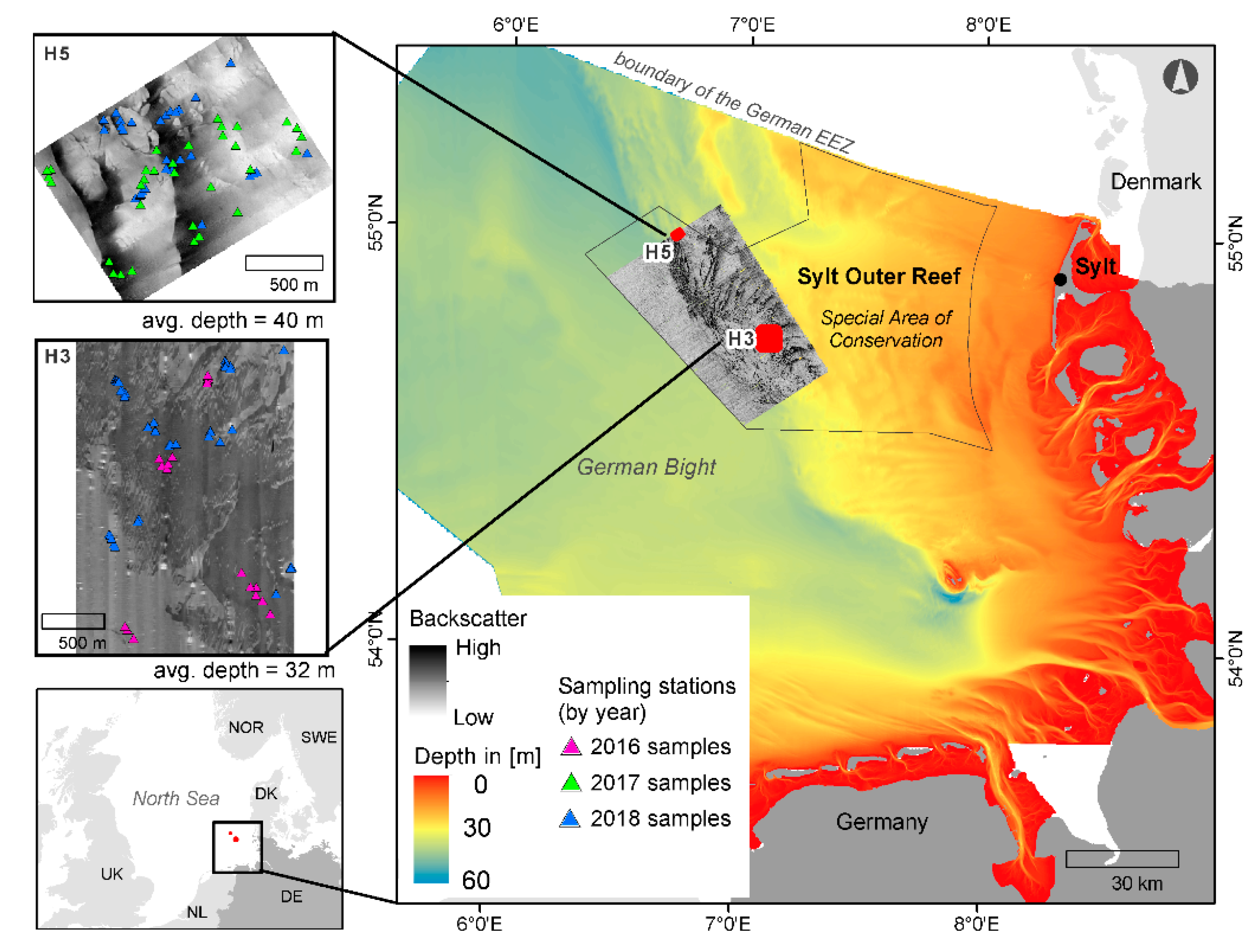
2.1. Study Site

We selected two relatively well-investigated areas within the Special Area of Conservation Sylt Outer Reef (SOR) (German North Sea). These areas, referred to hereafter as H3 and H5, are subsets representing the typical seafloor structure of the western Sylt Outer Reef and will be used to test the performance of our modelling approach (Figure 1). The areas have been the subject of the national seafloor mapping program SedAWZ, which is coordinated by the Federal Maritime Hydrographic Agency (BSH) [36,37]. Mapping of the SOR was given importance because of the complexity of the seafloor habitats (i.e., boulder reefs, gravel patches, and sands) in the area, which stands out in the relatively sand-dominated German North Sea. Semi- and fully-automated procedures for the detection of stones have been tested in area H3 [38] and sediment dynamics have been studied in both areas [39,40].
The German Bight is a relatively shallow water body with a maximum depth of about 60 m and represents the south-eastern part of the North Sea. Typical depth-averaged currents in the shallow part of the German Bight (depth < 20 m) are directed along the coast in a counter-clockwise direction, driven by tidal residual circulation enhanced by westerly and southwesterly winds (e.g., [41,42]).
Tidal dynamics, wave actions, wind-driven currents, and mixing determine the seabed sediment dynamics. The geomorphology and surface sediments of the Sylt Outer Reef is shaped by several glacial advances and retreats during the Pleistocene. Surface sediments consist of heterogeneously distributed coarse-grained lag deposits, which are mostly composed of siliciclastic material (reworked moraine deposits). The matrix grain size varies from coarse sand to gravel, which can also be mixed with pebble to boulder-sized particles. The coarse sediments are partly covered by Holocene marine fine- to medium-grained sands [43]. Parametric sediment echosounder data revealed that the lag deposits are submerged along the western boundary of the Sylt Outer Reef and form the eastern shore of the Paleo Elbe Valley [44]. The surficial finer sediments are deposited by a series of sedimentary infilling, which is driven by wind, waves, tides, and storm events during the Holocene Transgression [44].
Study area H3 is approximately 4.7 km2, characterized by one large elongated sorted bedform feature oriented towards the northwest –southeast direction. The bedform is visible in the side-scan mosaics as a high backscatter area (dark pixels; gray values = 55–255) and surrounded by low backscatter areas (light pixels; gray values = 0–54) (Figure 1, lower left box). Water depth ranges from 28 to 36 m.
H5 is a small area with a size of 1.8 km2, with two parallel bedform features with a north–south orientation (Figure 1, upper left box). Side-scan backscatter intensity is high (gray values = 55–255) in the southwest but gradually decreases towards the northeast (gray values = 0–54). The depth in H5 is slightly deeper than H3, with water depths ranging between 36 and 42 m. High backscatter areas were observed in deeper areas, while low backscatter regions dominated at shallow water depths [40].

2.2. Data Acquision and Processing

All data presented in this study were obtained during surveys performed between 2016 and 2018 in the two focus areas (Table 1). Focus area H3 was surveyed in October 2016 and March 2018 (17 months apart), while H5 was surveyed in November 2017 and March 2018 (4 months apart). Surveys were conducted with the German research vessel “Heincke” (Alfred Wegener Institute, Helmholtz Center for Polar and Marine Research, Germany).
Seafloor backscatter data was collected with an Edgetech 4200 MP side-scan sonar (SSS) (EdgeTech, West Wareham, MA, USA) at a frequency of 300 kHz and with a range of 75 m (H3) and 150 m (H5). The SSS was towed at a speed of 5 kn behind the vessel and was kept at 5–10 m above the seafloor. Surveys were designed to achieve a 10% overlap and 0.25 m along-track resolution of the SSS mosaics. Multibeam echosounder (MBES) data were simultaneously collected with a hull-mounted Kongsberg EM710 system (Kongsberg Maritime AS, Kongsberg, Norway). The MBES has two positioning units. The primary positioning system is from Trimble SP461 DGPS (0.5–3 m accuracy), while the secondary unit is DEBEG/Leica GPS (5–15 m accuracy). The very shallow mode with a frequency range of 65–106 kHz and pulse length of 0.2 msec, which is ideal for <100 m depth range [45], was used in our surveys. The default maximum reliable swath width was 90°. Side-scan data were processed using the QPS Fledermaus Geocoder Toolbox v.7.8.8 software (Quality Positioning Services BV, Zeist, the Netherlands) to reduce the artefacts in the raw data and produce SSS mosaics that were compatible for change analyses (see [40] for details on the procedure). The process applied backscatter, beam pattern, and angle-varying gain corrections, and improved the spatial accuracy of the SSS mosaics (spatial accuracy: ±0.25 m). The SSS mosaics were gridded to 0.25 m resolution with decibel(dB) values cropped to a ±3σ dB range and logarithmically mapped to an 8-bit scale. Post-processing of MBES data was conducted in QPS Qimera v2.0.1 software (Quality Positioning Services BV, Zeist, the Netherlands) to correct the raw MBES data from tidal effects and reject invalid soundings. The survey track distances, designed for SSS-survey, were too wide to achieve a swath overlap of the MBES data. Hence, the gaps in bathymetric data (~30–100 m apart) were interpolated to generate a digital elevation model (DEM) using the Topo-to-Raster function of ArcGIS v.10.7.1(Environmental Systems Research Institute-ESRI, Redlands, CA, USA), which is an interpolation method specifically designed for the creation of hydrologically correct DEM.
Ground-truth information was collected from both underwater video and sediment grain-size sampling (Table 1). Underwater videos were obtained using a Kongsberg OE14-366 Color Zoom Camera (Kongsberg Maritime AS, Kongsberg, Norway; horizontal Resolution 460/470 TV lines) and a GOPRO 3+ Black Edition (GoPro, Inc., San Mateo, CA, USA; resolution: 1920 x 1440, 47.95 frames per s). The cameras were mounted on a robust metal frame with a laser scale (spacing: 10 cm). The GPS system of the research vessel was connected to the on-board control unit of the camera for geographic referencing. The cameras were deployed underwater as close as possible to the seafloor surface for at least five minutes and towed while the ship was drifting at a speed of less than 1 kn. Videos were initially screened for image quality to omit blurred footage. The remaining videos were then converted into individual images at two-second intervals using the scene video filter of the VLC media player (VideoLan project, version 3.2.1.0). Subsequently, photos with a clear image of the seafloor were selected manually and the coordinates were recorded.
Sediment samples were collected with a Van Veen grab sampler (HELCOM standard). Sites for sampling were selected based on their backscatter characteristics in the SSS mosaic of the study area, which was processed on-board upon acquisition. In the home laboratory, carbonate and organic matter were removed from the sediment using chemical treatment according to the procedures described in [46] and analyzed using a CILASS 1180 L laser particle sizer (LPS, range: 0.04–2500 µm). Particles larger than 2000 µm were removed by sieving before measurement. Grainsize statistics were calculated in GRADISTAT v8.0© [47].
All samples including the grain size data were categorized according to Folk and Ward’s [48] and BSH [36] sediment classification as: sand, coarse sediment (gravely sand, sandy gravel, and gravel), and lag sediment (sediments of different grain size with gravel and stones). The Level A category of the BSH sediment classification scheme, which encompasses different sediment types, was used to classify our ground-truth samples (Table 2). However, the backscatter properties of the sand class in the SSS mosaics of H3 and H5 are different. Sand was reflected as medium-high backscatter in H5 rather than the low backscatter in H3 (Figure 2, Figure 3 and Figure 4). Hence, we differentiate the two sand classes based on their backscatter properties: sand low-backscatter (SLBS) and sand high-backscatter (SHBS).
In total, 106 ground-truth samples (both sediment and video stills) were obtained at H3, while 76 samples were collected at H5 (Table 3). However, it must be noted that only a subset of the total ground-truth samples from each study area was used in each model run (Table 3).

2.3. Modelling Approach

The idea of our approach is to predict each sediment class separately using ensemble modelling and then combine the resulting class-specific predictions into a sediment distribution map. In this regard, different models were built for each sediment class per study area. Additionally, we developed models for each year of the datasets to evaluate the changes in sediment distribution. We modelled eight different datasets in total.

Ensemble Modelling

Ensemble models predict distributions of the response variable (i.e., sediment type) by combining different modelling techniques to derive a general prediction.
Here, we utilized the ‘BIOMOD2′ package within the statistics software R (CRAN) v.4.0.3 [24,49] to perform ensemble modelling. BIOMOD2 is the updated object-oriented version of the BIOMOD package and has been developed for ecologists to predict species distribution, but can also be used to model any binomial data (i.e., binary presence–absence object) in function of any explanatory variables [24]. BIOMOD2 has been used to predict macroalgal habitats [50], to map the distribution of medicinal plant species [51], and for ecological niche modelling of basking sharks [52], but it has not been applied to predict seafloor sediments.
Four machine-learning approaches that are commonly used in seafloor mapping were selected from the BIOMOD2 package: classification tree analysis (CTA), artificial neural networks (ANN), random forest (RF), and generalized boosted models (GBM). In CTA, a decision tree is grown by repeatedly splitting the data and then the complex tree is pruned back to the desired size using specific rules to reduce overfitting [53]. In ANN, models were run several times and the mean prediction was used or the best fitting model was selected [23]. It uses sets of adaptive weights to link the response to the predictors [25]. RF grows each tree with a randomized subset of predictors and several trees are grown as the predictors are aggregated by averaging [53]. Lastly, GBM uses a forward stage-wise procedure that iteratively fits simple trees to the training data, while gradually increasing focus on poorly modelled observations [25]

2.4. Input Data for the Models

2.4.1. Sediment Data

The sediment and video sample data were converted into points and binary format for the model. For example, locations in which sand was observed were assigned 1, while areas in which there was no sand i.e., the location was categorized as pseudo-absence or as another sediment class based on the sediment samples, were assigned 0. Pseudo-absences are artificial absence data, which represent places in which the response variable is supposed (but not confirmed) to be absent [54,55]. Pseudo-absences data was built for each sediment class because most of the models require both presence and absence data. To generate pseudo-absences, we conducted three iterations using random strategy with a selection of 200–500 pseudo-absences to prevent sampling bias [25].

2.4.2. Predictor Variables

Geophysical and textural features were extracted from processed MBES and SSS data, and from oceanographic models that were developed for the German Bight. These features were then used to predict the probability of occurrence of each sediment class. A total of 348 predictor variables were generated for this study.
Bathymetry, slope, northing, and easting were derived from our MBES data using the Benthic Terrain Modeler v3.0 Toolbox of ArcGIS 10.7.1 [56]. Spatial data on near-bottom (averaged over 1 m-layer above the seabed) tidal residual currents and tide-induced maximum friction velocities were derived from the barotropic multi-layer setup for the south-eastern North Sea. The FESOM-C coastal ocean model was used as a numerical tool. It was validated through a series of experiments with a particular focus on the North Sea area and its tidal dynamics in particular [57,58,59].
Textural features of the SSS mosaics were extracted using the gray-level co-occurrence matrix package in R (GLCM v.1.6.5.) to identify the spatial characteristics of the mosaics. GLCM evaluates the co-occurrence of pixel gray-level values at given offsets to enhance image classification [60,61]. We applied gray levels of 32, window sizes of 9, and inter-pixel distances of 5 and 10, which are the recommended settings for GLCM analysis using SSS data [19]. Feature calculation was conducted on different orientations: 0°, 45°, 90°, 135°, and the mean of all directions. A total of 80 statistical features were extracted for each side-scan mosaic. The list of the calculated GLCM statistics and geophysical features used in this study can be found in Supplementary Table S1.

2.4.3. Feature Selection

The combination of few presence data and many predictor variables can easily cause model overfitting [62]. In addition, correlation between two or more predictor variables in a statistical model can induce multi-collinearity [63]. Therefore, as we are working with a small number of occurrences, the selection of predictor variables is an important step in our approach. A general rule of thumb is the 1:10 ratio of presence data and predictors, which means to include only two predictors for twenty presence data points [62,64].
Predictor variables were selected in an iterative process. Initially, the variance inflation factor (VIF) was used to detect collinearity between predictors and to remove redundant variables. The VIF is based on the square of the multiple correlation coefficient (R2) resulting from regressing the predictor variable against all other predictor variables [63]. A VIF greater than 10 indicates a collinearity problem [65]. Here, VIF analysis was performed using the ‘vifstep’ function in the R package ‘usdm’ [66]. All predictor variables were analyzed in a stepwise procedure, whereas variables with VIF of >5 were removed. Further feature selection was conducted during model calibration based on the variable importance score of the predictors. In the BIOMOD2 package, the variable importance function uses a machine-learning approach to randomize one of the variables in each permutation and calculate a correlation score between the standard prediction and the new prediction. The higher the value, the more importance the predictor variable has on the model.
The variable importance score was calculated through 10 permutations and predictor variables with a low mean variable importance value (≤0.1) were excluded from the modelling. The variable importance score of the predictors that were used in our models are presented in Supplementary Table S2.
We have set a maximum of five predictors to model each sediment class and avoid model overfitting and multicollinearity.

2.5. Model Calibration and Validation

The parameters and complexity of each model were modified depending on the sediment class, number of predictor variables, and presence data.
Initially, single models (i.e., RF, CTA, ANN, and GBM models) were calibrated using 70% of the presence data and validated with the remaining 30%. The cross-validation procedure was repeated 20 times for each model. During calibration, the settings and complexity of the single models were repeatedly modified until the optimal TSS value (≥0.7) was achieved. Model performance was assessed by the threshold-independent receiver operator characteristics (ROC), threshold-dependent true skill statistics (TSS), and Cohen’s Kappa [67]. TSS ranges from −1 to +1, where +1 indicates perfect agreement and values of zero or less indicate a performance no better than random. This is different from Kappa because TSS is not affected by the size of the validation set and prevalence. A TSS score of 0.7 or higher indicates good or exceptionally good performance of the model [68]. ROC assesses the relationship between the false positive fraction (specificity) and the sensitivity for a range of thresholds. Kappa indicates the best possible agreement [68].
Subsequently, only single models with a TSS value of ≥0.7 were included in the ensemble model of each sediment class. TSS is used to select the ‘‘best’’ model, i.e., the model providing greater accuracy on the test data for sediment class. Ensemble models were calculated based on the committee average, mean, and coefficient of variation of the model predictions (Table 4). Here, we used the committee-averaged ensemble models to build the sediment distribution maps because it gives both the prediction and measure of uncertainty. In committee averaging, each model decides whether the sediment class is either present or absent, and then the sum is divided by the number of models. For example, when the prediction is around 0.5, it means that half of the models predict 1 and the other half predict 0 [24,25]. Moreover, to remove the bias across the selected models, BIOMOD applied the same weight to all predictions to derive a consensus prediction. The weights are calculated based on models’ predictive accuracy on test data [24].
As a result of multiple model parameters, a total of 240 models were built for each sediment class (4 algorithms x 20 cross-validation runs x 3 pseudo-absences sampling). A total of 960 single models and eight (8) ensemble models were generated for the two study areas (Table 4). The R script used to perform the ensemble modelling can be found in Supplementary Material 1.

2.6. Ensemble Mapping and Map Accuracy Assessment

The committee-averaged ensemble predictions for each sediment class were aggregated to create an ensemble map. The procedure was conducted using the raster analysis tools of ESRI ArcGIS 10.7.1 and is explained in Appendix A. In summary, we used the maximum cell values of each sediment class as the parameter to combine them into one map. The output is an ensemble map of the predictions where the most probable class was assigned to the location.
The accuracy of the ensemble maps was calculated using the ‘confusionMatrix’ function of the ‘caret’ package in R [69]. A separate testing dataset, including 30% of the presence data of each sediment class per year, was used to extract the predicted values in the ensemble maps in the location of the testing data, after which a confusion table was constructed to calculate statistics such as overall accuracy. The overall accuracy indicates the percentage of areas that were correctly predicted. The Kappa coefficient, a commonly-used accuracy index in seafloor mapping, was also calculated but was not used to evaluate the accuracy of the ensemble maps, because recent findings suggest that it is an inappropriate index to describe the classification accuracy of thematic maps obtained by image classification [70].

2.7. Detecting Changes in Seafloor Sediment Maps

To determine if there are changes in the seafloor sediment maps of different years, we applied the change detection method for habitat classification maps of Rattray et al. [71]. The method uses a transition matrix that is a conventional method of assessment of land cover changes [72,73]. In this method, the two sediment classification maps from different years were cross-tabulated to derive the statistics that describe temporal changes (i.e., net change, persistence, etc.). In recent years, it has been adapted to detect changes in benthic habitat maps and seafloor sediments [19,71,74].
The ‘from-to’ transition of the sediment classes, persistence, and amount of gain/loss were calculated for H3 and H5. Gain refers to the increase in the area coverage of a given class, while loss refers to the decrease. Persistence indicates no change in the sediment class [71,72].

3. Results

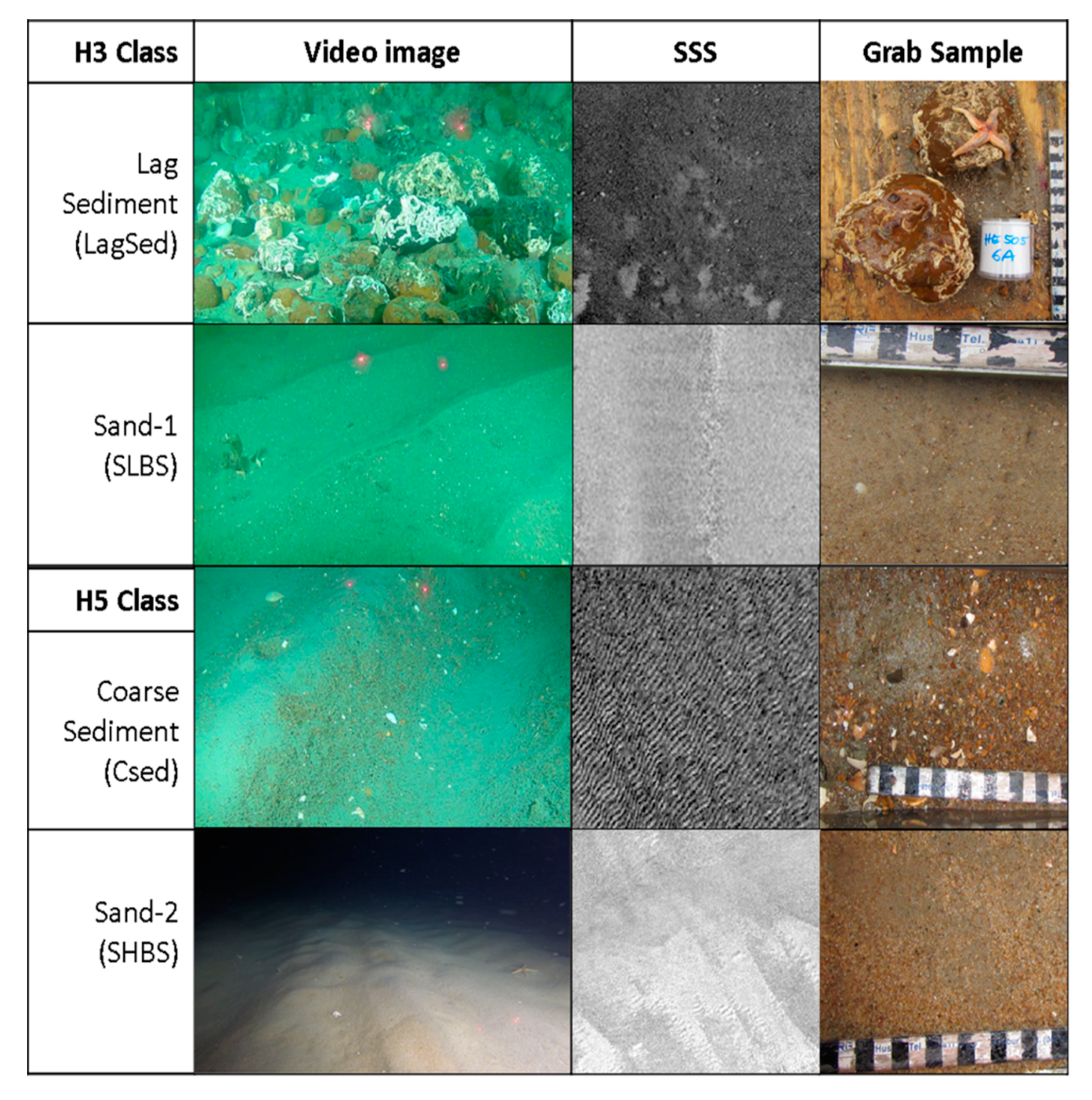
3.1. Sediment Classes Based on Field Survey

According to grab samples and underwater videos, lag sediments (LagSed) and sand-1 (SLBS) were the sediment classes in H3 (Figure 2 and Figure 3). Lag sediments were observed in high-backscatter areas (dark pixels) and as clusters and patches of gravel, cobbles, and boulders with attached biotic species (Figure 2). SLBS class areas were observed in low backscatter zones (lighter pixels) and were seen as small oscillation ripples (~10 cm wavelength) in the underwater videos (Figure 2).
We have identified two sediment classes from our survey data in H5, namely coarse sediment (CSed) and sand-2 (SHBS) (Figure 2 and Figure 4). CSed was observed in high-backscatter areas in the SSS mosaic (Figure 4). In the underwater images, the CSed class is characterized by bedforms with coarse sediments and shell fragments on the lee slope. Conversely, the SHBS class is reflected as medium-high backscatter in the SSS mosaics (Figure 4). When viewed at 25 cm-resolution of SSS data, the SHBS area shows presence of ripples with approximately >20 cm of wavelength. This was subsequently verified in the underwater images as bedforms with shell fragments and coarser sediments on the troughs (Figure 2).

3.2. Ensemble Model Performance

Of the 240 individual models that were created, only models with a TSS value of >0.70 were included in the final ensemble model, which was used to predict the sediment classes (Table 4). The predictive power and accuracy of the ensemble models are excellent with high statistical reliability (TSS > 0.8/ROC > 0.9) (Table 5). The agreement between the response and explanatory variables was also good (Kappa= 0.4–0.9).
Based on the TSS and ROC scores of the four algorithms, GBM and RF performed the best in predicting coarse sediments (LagSed and CSed), while ANN and GBM predicted sand very well. CTA had the poorest performance in predicting sediment classes with a small sample size and few predictor variables. However, despite the poor performance of the CTA algorithm, it was still able to generate models with TSS scores of 0.7 that were included in the final ensemble. We observed that using only two to three models, rather than four, decreased the predictive accuracy of the ensemble model.
The importance of the predictor variables in predicting performance of the algorithms is listed in Supplementary Table S2. Briefly, GLCM variables such as correlation, second moment, homogeneity, and contrast highly influence the predictive performance of the model. Side-scan mosaic, slope, and easting are also important predictor variables. Notably, we found that SSS mosaic and slope can predict sand areas very well, while the GLCM features of the SSS mosaic can discriminate LagSed and CSed areas.

3.3. Seafloor Sediment Distribution in H3

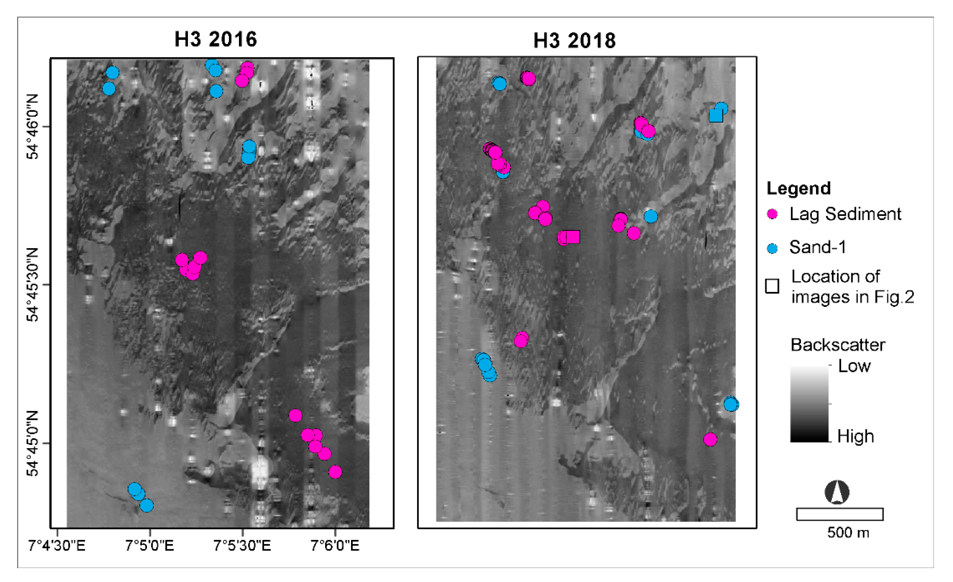
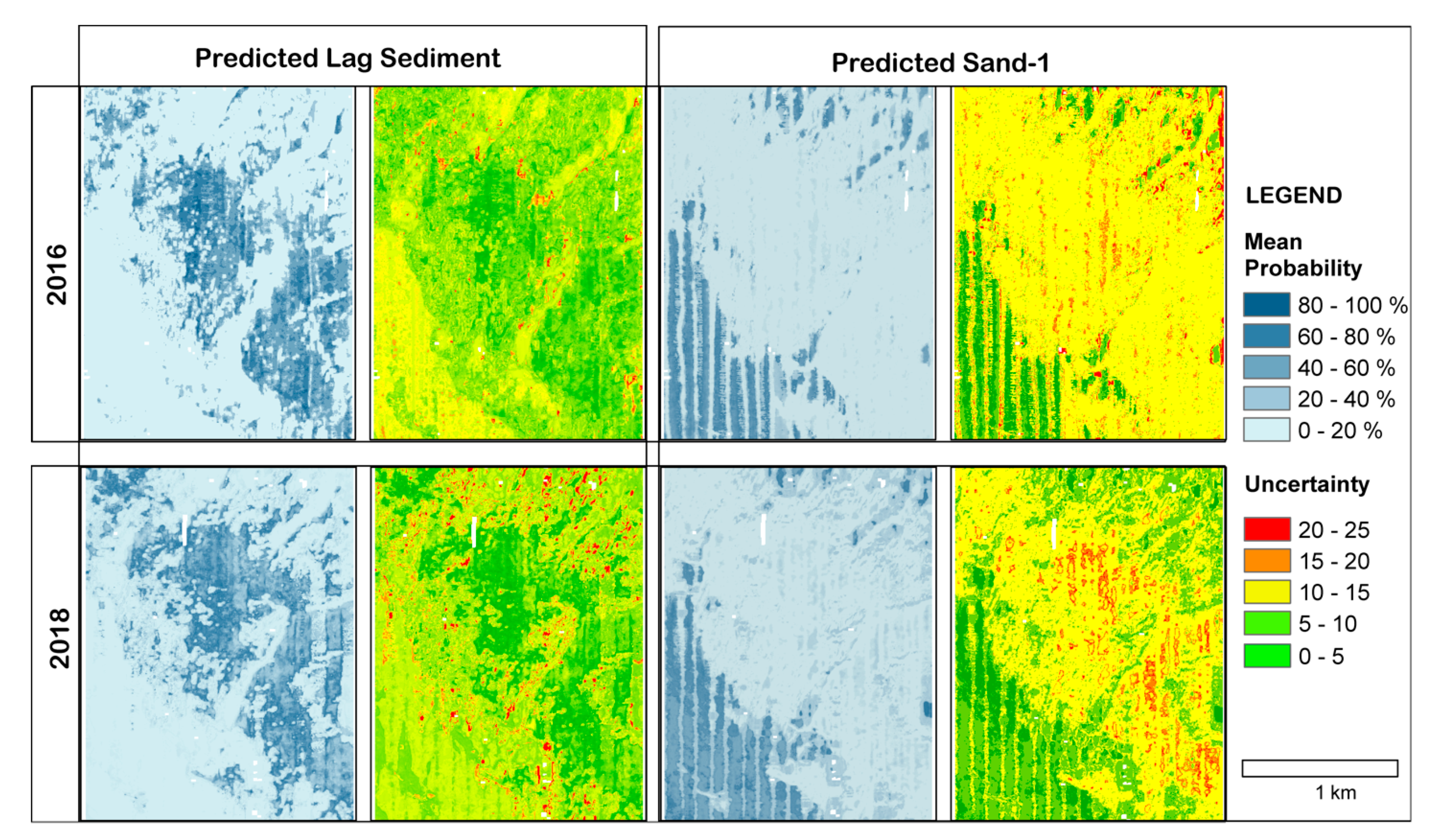
3.3.1. Predicted Sediment Distribution in 2016 and 2018

The ensemble models have predicted around 41% of the total area of H3 (1.92 km2 of 4.71 km2) to be LagSed (TSS = 0.91, Table 5) and the remaining 59% of the area as Sand-1 (TSS = 0.85–0.90) based on the 2016 dataset (Figure 5, Table 5). LagSed was predicted with high accuracy (TSS = 0.91, Table 5) within the sorted bedform area. SLBS surrounds the bedform feature in the southwest and northeast (Figure 5 and Figure 6).
According to the 2018 dataset, the area of LagSed had slightly increased in 2018 from 41% to 49% of the total area (Figure 5). Sand dominated 51% of the area around the bedform and some small patches of sand were located within it (Figure 5). The accuracy is reliable except inside the bedform area, in which the predictions seem to be artefacts from the side-scan mosaics that were used as input data in the models; hence, they were excluded in the committee-averaged predictions (Figure 6).

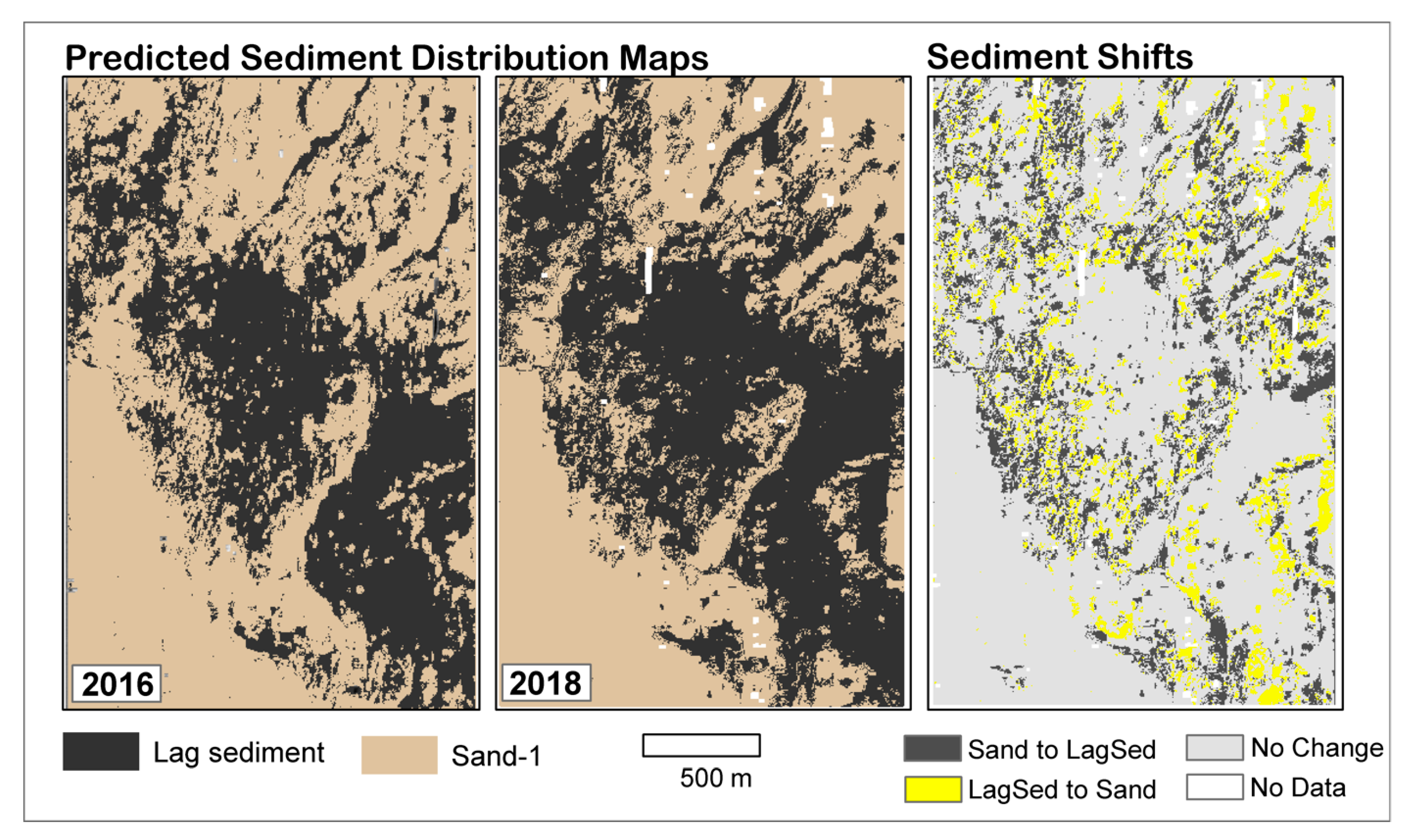
3.3.2. Seafloor Sediment Distribution Maps of H3

Overlaying the class-specific predictions into one map based on the percentage of their probability of occurrence have resulted in a statistically reliable seafloor sediment map with an overall accuracy of 100% (Table 6, Figure 6). Both maps were able to classify the high backscatter bedform as LagSed and its surrounding area as sand (Figure 6).

3.3.3. Changes in Seafloor Sediment Distribution Maps of H3

The transition analysis of the seafloor sediment maps in H3 showed that most of the changes within the 17 months had happened around the boundary of lag sediment and the sand-1 (SLBS) class area (Figure 6). Lag sediment class was more affected by the transition than the surrounding sand areas that were mostly unchanged (persistence = 2.03 km2 of 4.71 km2) (Table 7).
Along the boundary of the two classes, we noticed that most sand class shifted into the LagSed class, particularly in the northeast and southwest portion (Figure 7). Moreover, most of the sand-to-LagSed transitions occurred within the bedform area. This transition had caused a 16.3% increase in the area coverage of LagSed in 2018 and resulted in an 8% loss of the sand class area in the map (Table 7). However, this loss for sand class is lower than its 43% area coverage, which had remained unchanged for two years.
Overall, 2.26 km2 (48%) of the map had changed in 2018, where LagSed was the most affected class.

3.4. Seafloor Sediment Distribution in H5

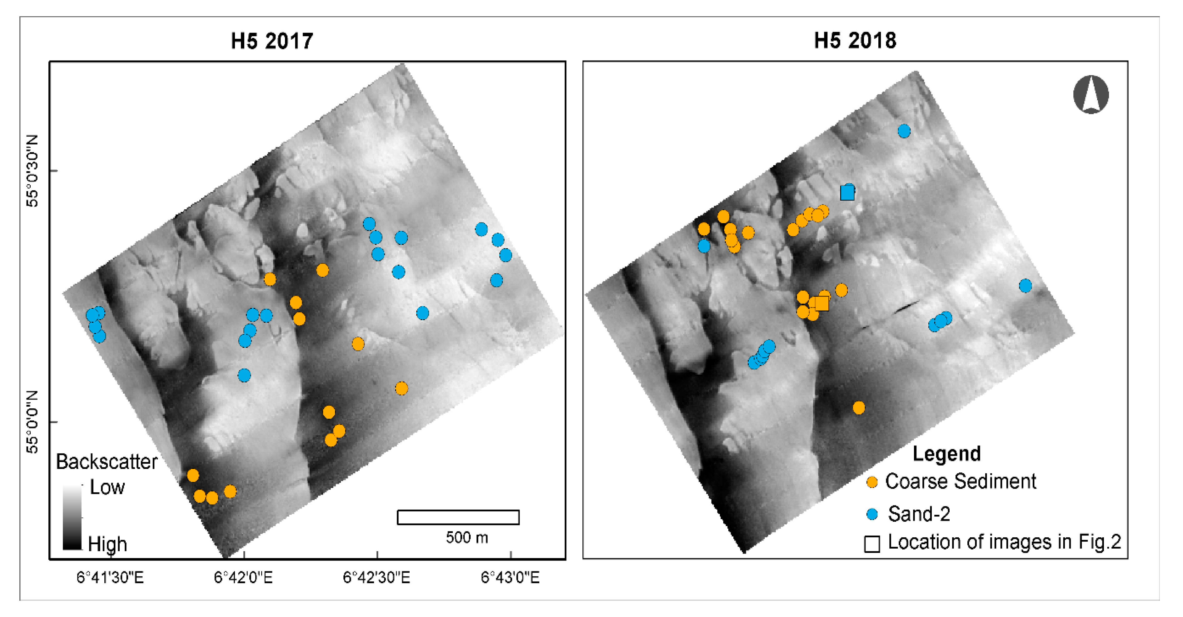
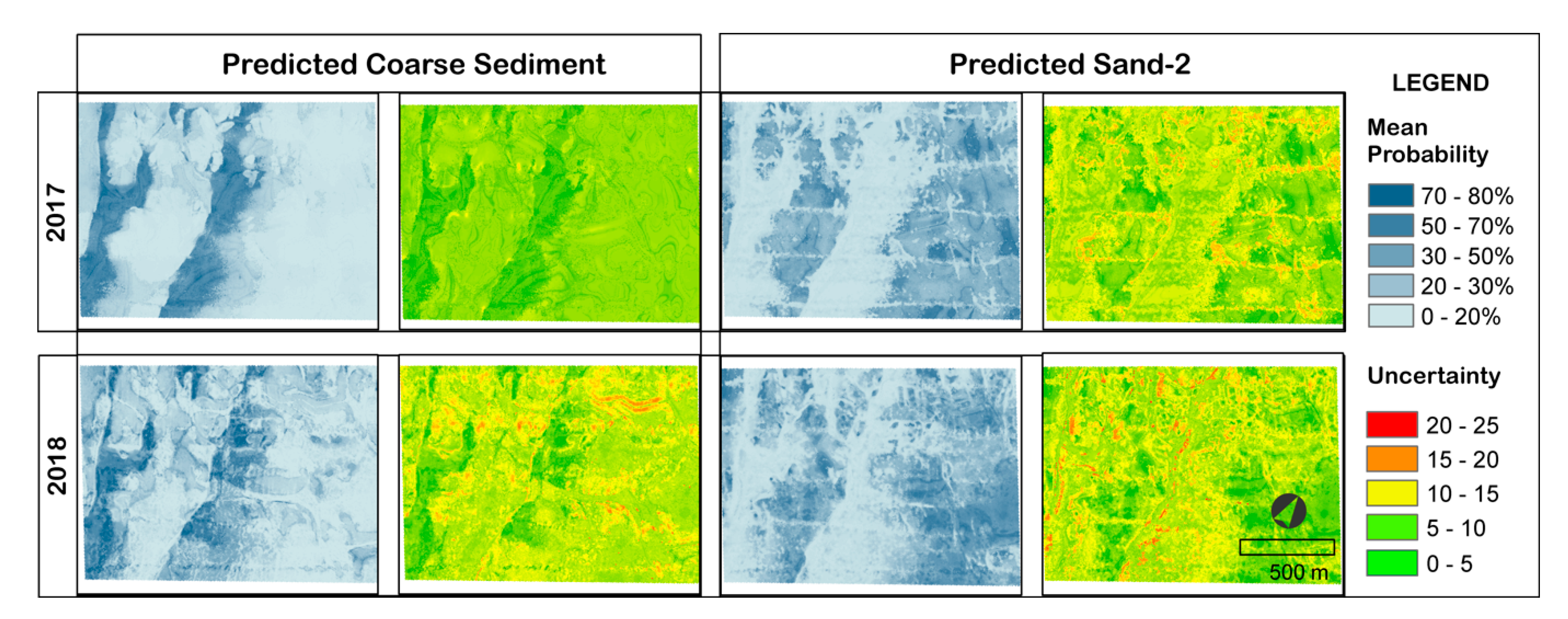
3.4.1. Predicted Sediment Distribution in 2017 and 2018

The two parallel bedform features in H5 were predicted as the CSed class, while the surrounding areas were classified as Sand-2 (SHBS). Some areas outside the features were also predicted as CSed especially in the 2018 map but the accuracy of this prediction is low (Figure 7).
In 2017, the two features have been predicted as CSed with good accuracy (TSS = 0.82, Table 5). However, some areas in the northeast of the bedforms were not classified (Figure 7). Around 63% of the total area of H5 (1.81 km2) was predicted as SHBS and only 37% was predicted as CSed. The prediction of SHBS in 2017 is particularly good (TSS = 0.90) (Table 5, Figure 7).
In 2018, some areas in the northeastern portion of H5 were predicted as CSed (TSS = 0.86, Table 5) but with higher uncertainty (Figure 7). The prediction has also more visible noise or artefacts compared to the 2017 modelled data. The prediction of SHBS in 2018 has lower probability than in 2017 (TSS = 0.83) (Figure 7). In both maps, the CSed class is well-defined in the southwest but seems to fade towards the northeast.

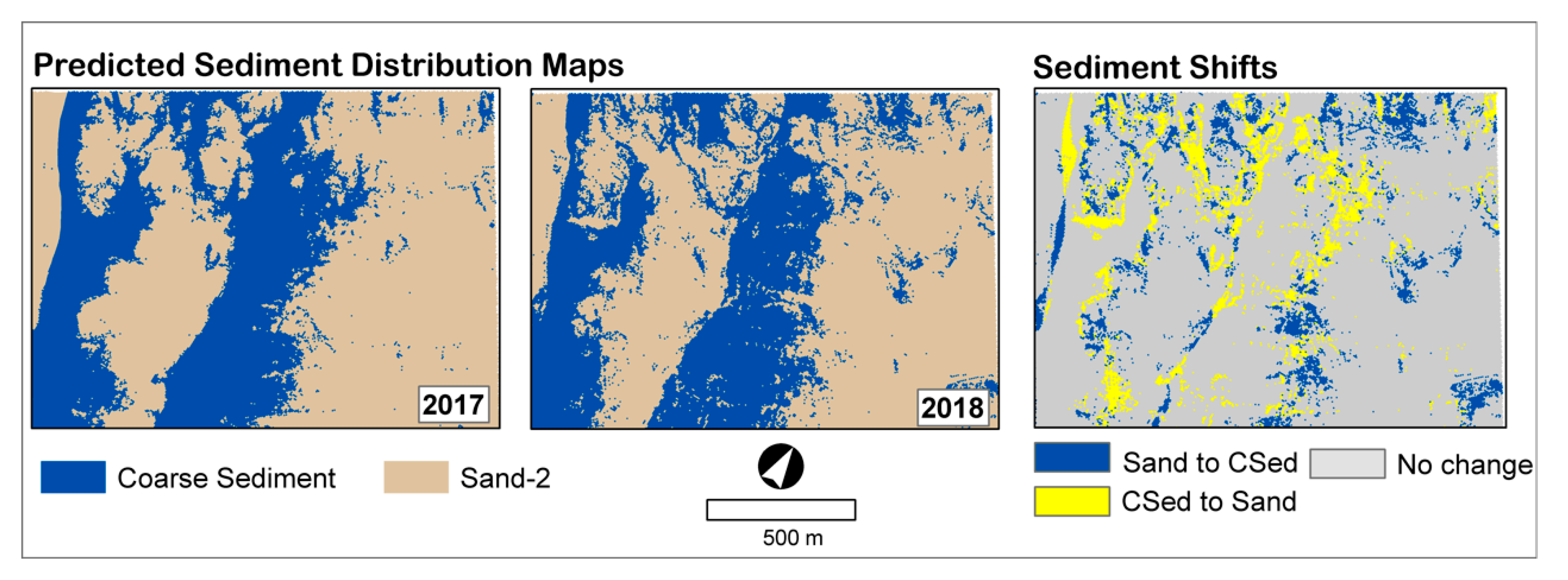
3.4.2. Seafloor Sediment Distribution Map of H5

The ensemble maps of H5 have both received a comparable and good statistical score (Figure 8 and Table 6). Despite the artefacts in the original data (Figure 4), the 2017 map still obtained a 94% overall accuracy (Table 6, Figure 8). The 2018 ensemble map has a lower but still good accuracy of 86%, which indicates that the observed data (ground-truth) were classified correctly (Table 6, Figure 8).
Although, interpretation of the map must be done with care because of the artefacts in the raw data. The final ensemble maps (Figure 8) can be used to guide the interpretation if map accuracy is the main concern. These maps were generated using the committee-averaged ensemble models, of which the areas with high uncertainty were excluded in the final prediction.

3.4.3. Changes in Seafloor Sediment Distribution Maps of H5

By 2018, 35% (0.63 km2) of the 2017 sediment distribution map had changed within four months. These changes were observed along the boundary of the classes and in the north-northwest portion of H5 (Figure 8). However, both sediment classes have gained and lost almost the same amount (Table 7). For example, CSed gained 8.72% of area coverage in 2018 from SHBS but also lost 8.68% of its area to SHBS in the same year.
We observed that the CSed-to-Sand class transition mainly occurred in the north- northeast facing side of the bedforms and the CSed class gained more area in the northwest (Figure 8).
Overall, the CSed class transitioned the most (29%) and ~54% (0.98 km2) of the SHBS class area remained the same.

4. Discussion

4.1. Predicting Seafloor Sediments with Limited Ground-Truth Samples

The accuracy of the predicted seafloor sediments in a heterogenous area such as the Sylt Outer Reef can be influenced by several factors that may negatively influence the results of the modelled sediment distribution maps [30]. These factors include (1) an inadequacy of the selected classification system, (2) a low discriminatory power of the predictors, or (3) a mismatch between the response (i.e., grab sample) and predictor variables (e.g., backscatter mosaic). In addition, an unequal number of samples between sediment classes may result in under or overpredictions in the modelling results [52]. Furthermore, discrepancies between different techniques can be very large and some models may be more sensitive to sampling bias, which might reduce model transferability and selection [24,62,75]. These issues can be alleviated by creating an ensemble map that aggregates individual predictions into one map and by adopting a class-specific modelling approach that models the spatial distribution of grain-size classes without bias to the dominant class [11,30,34]. Moreover, ensemble modelling can compensate for unwanted inter-model variability and model selection bias by aggregating the results of multiple models into one general prediction [24,25].
The probability of occurrence of different sediment classes was modelled for two different locations and different temporal scales. In this regard, we first assumed that we would produce highly variable results but we achieved comparable outputs. For example, GBM and RF models were able to predict coarse sediments (i.e., LagSed and CSed) in both H3 and H5. Moreover, there have been similarities in the important variables that predict specific sediment classes (Supplementary Table S1). In this regard, we have tested the potential of our approach to different study areas, different spatial scales (larger or smaller scale), and for repeated surveys.
However, the most important factor that influenced our results is the quality of input data. Environmental predictor variables influence the probability of occurrence [25]. As we have seen, the nadir artefacts from the SSS mosaics were reflected in the probability of occurrence maps (Figure 5 and Figure 7). This implies that the quality of the data is important when performing our methodological approach.
In addition, we observed that the spatial distribution of the ground-truth samples highly influenced the prediction. This issue was addressed by generating three sets of randomly selected pseudo-absences, which substantially improved the model predictions. In species distribution modelling, pseudo-absences are meant to be compared with the presence data and help to differentiate the conditions under which species can occur or not. Therefore, selecting the appropriate number and strategy of generating pseudo-absences may optimize model performance [55].
In this regard, survey design is important before collecting field data to ensure that all samples for each sediment class are well-distributed (spatially). The outputs of this study can be utilized for this purpose. For example, the probability of occurrence and uncertainty maps can guide scientists or seafloor mappers to guide the sampling campaign and thus make the survey more precise and time efficient.
Overall, predicting multiple sediment classes one-by-one using ensemble models has improved the accuracy of our predictions. The class-specific modelling approach (i.e., classifying the classes one-by-one) has improved the predictions because it lessens the bias to the dominant class and reduces the effect of data imbalance. This approach differentiates our study from other studies on sediment mapping, which applied ensemble modelling and supervised classification methods but modelled multiple sediment classes at the same time [11,12,13,17,21,30,31].

4.2. Seafloor Sediment Distribution in the Sylt Outer Reef from 2016 to 2018

Sediment distribution is an important parameter for the understanding of benthic habitats, the management of maritime economic activities, and the monitoring of impacts of human activities on the seafloor [9,76,77]. We predicted and mapped the possible seafloor sediment types for two areas in the Sylt Outer Reef Special Area of Conservation.
In H3, the bedform feature was predicted to be composed of lag sediments and surrounded by sand. Among the two sediment classes, the LagSed class was more affected by sediment shifts that occurred within the bedform area. We observed that more of the LagSed class appeared especially nearby the boundary of the bedform, while more of the sand class was seen inside the bedform after two years. Boundaries of the bedforms were observed to be the most vulnerable to sediment shifts [39,40,78,79,80]. In contrast, the surrounding sandy areas seemed to be stable over the period of observation.
The sediment class in H5 was more difficult to predict than in H3 because of the mismatch of the ground-truth data with the predictor variables (acoustic data). For example, areas that were interpreted to be sand based on grain-size analysis appeared as areas with medium-high backscatter strength (dark pixels), rather than showing low backscatter strength (light pixels) as for the sandy area in H3 (Figure 3). The stronger backscatter response of the sandy area can be explained by the more varied morphology and sediment composition of H5, as observed in the underwater videos (Figure 2). In some parts of the sandy areas of H5, the seafloor was characterized by the presence of small wave ripples (>20 cm wavelength) and was partly covered by coarse sediments (Figure 2). Moving a few meters away from the wave ripples, the seafloor became dominated by small ripples and finer sand fractions. These variations in seafloor roughness influenced the backscatter intensity that was recorded by the sonar. Rough and hard surfaces return high backscatter intensity, while smooth and soft surfaces send low backscatter intensity to the sonar [81,82]. As a result, the sandy areas of H5 appeared as patches of medium-high backscatter in the SSS mosaics, in contrast to the low backscatter response of the sandy areas in the H3 mosaics (Figure 2).
As seen in H3, shifts in sediment class occurred along the boundaries of the two bedforms in H5. Although the quantity of transition between the two classes are almost the same, it does not imply that changes did not occur but rather signifies that the intensity of changes are low. Shifts from the CSed class to the SHBS class occurred at the northeast-facing side of the bedform features, while Sand-to-CSed transitions were observed in the north-northwest area of H5.
In summary, sediment shifts were observed along the boundaries of the bedform features but the morphology of the bedforms were relatively stable: no additional bedforms or drastic changes were documented. These findings are in accordance with our previous study [40] and with other studies on changes in sediment distribution in the North Sea, in which the gravel/coarse substrates and fine substrates fluctuated but overall were stable [39,74,83]. In our previous study, we monitored the boundary lines to detect sediment shifts, but here we looked at the changes in the modelled sediment distribution maps. The results of both studies are comparable, i.e., the sediment shifts were mainly observed in the northeast and southwest direction of the bedforms. The spatial sediment transitions that we detected in this study may be attributed to the fluctuations of the sandy materials along the boundary. The deposition or erosion (winnowing) of mobile sand fractions covers or uncovers the coarser sediments underneath, which is largely driven by tidal currents and storm events [39,40,80]. The mobilization of sandy materials along the boundary caused the oscillation of the boundaries rather than moving the boundaries in one direction [40].

4.3. Sediment Transitions and Their Implications

Monitoring changes in sediment distribution maps is especially important in areas with heterogenous seafloor cover, for which tidal currents, wave actions, and wind-driven flows determine the seabed dynamics and may induce drastic changes in the sediment distribution pattern [30,74,84]. Moreover, sediment transition can be used to predict species responses to habitat change [1,3,4,85]. Changes in sediment composition along sediment gradients/boundaries can alter the behavior and distribution of benthic species. For example, the loss of coarse sediments forced benthic invertebrate communities to leave their habitat and move to fine sediments, which consequently changed the community compositions (taxa presence and absence) [5]. In addition, changes in detrital resources (i.e., coarse sediments), which serves as a refuge in soft sediment systems, causes decline in macroinvertebrate species [6]. Therefore, the monitoring of changes in seafloor sediments is vital for the conservation of benthic biodiversity and detrital resources, especially for important marine protected areas such as the Sylt Outer Reef.
Accurate prediction of sediment class is necessary to be able to detect the actual seabed change in a highly complex area [30,74,84]. In this regard, sediment distribution maps need to be updated to develop and implement appropriate strategies to manage maritime activities and marine conservation areas. However, the question concerns how often we must update these maps.
In this study, the sediment transitions imply that sediment dynamics in the western part of the Sylt Outer Reef are highly active and can cause conceivable changes in the sediment distribution maps in a short period of time. For example, approximately 48% of the sediment distribution map of H3 appears to have changed after two years, while 35% of the maps in H5 experienced changes in just four months.
Therefore, in areas of the Sylt Outer Reef with seafloor features such as in H3 and H5, seafloor monitoring can be conducted at approximately no more than 5 years because by then, the sediment distribution may have changed substantially at the boundaries of the features. This approximation is based on our findings for the two sites in the Sylt Outer Reef, in which we observed that this survey interval is necessary to provide reliable recommendations for monitoring purposes. Moreover, to find out whether the observed changes have happened constantly between the studied time periods or because of an extreme event (e.g., severe storms), additional surveys ideally before and after a storm are necessary. The surveys can verify the actual cause of these changes and evaluate the impact of storms to the sediment distribution pattern.
Seafloor dynamics are likely to be as variable as tidal currents or ocean climate patterns and thus a regular interval (i.e., 5 years) may miss important dynamics. However, monitoring a large area can be time consuming and costly. In this regard, repeated monitoring of subsets of areas, as in this study, can be an alternative to evaluate seafloor changes until it becomes evident that a new “full” survey is necessary. Moreover, as coarse sediments (i.e., LagSed and CSed) in the German Bight are important habitats for epibenthic assemblages and sediment transitions can have adverse effects in their ecosystem, mapping these areas is important for habitat monitoring and conservation efforts [38,85].

4.4. Outlook

Information on sediment distribution was found to be a very good predictor of benthic species densities and distribution [8,50,86,87]. Hence, our modelled prediction of sediment distribution can be used for marine conservation studies as input for species distribution modelling [1,50,87] and for monitoring of the impacts of human activities [2,9,76,88].
Moreover, the seafloor sediment maps that were generated in this study can provide information for future seafloor mapping efforts. The maps can be used by seafloor mappers in planning their survey and to design a systematic ground-truth sampling approach, which may improve the accuracy of the seafloor sediment maps in the future.
In this study, we utilized bathymetric derivatives from BTM, hydrodynamic models, and textural features from SSS backscatter to predict sediment distribution. Another approach that can be explored in the future is to incorporate other predictor variables to model sediment distribution from MBES data, such as spectral features from dual-frequency MBES [89], marine geomorphometry features [90], and features from angular response analysis of MBES backscatter [91]. Moreover, the methods performed in this study can be tested to model multiple sediment classes (i.e., more than two) and to test its applicability to a larger spatial scale.
Furthermore, the methodological approach that we presented can also be applied to other types of underwater exploration studies in which ground-truth data is scarce, such as reef mapping [12], deep-sea sediment mapping [15], habitat modelling in remote areas [50], and to detect sunken structures for underwater archaeology [92]. Hence, the methods in this study can be adapted not only by geologists but also by biologists, ecologists, archaeologists, and environmental scientists.

5. Conclusions

In this study, we tested the capacity of class-specific ensemble modelling using BIOMOD2 as a reliable and reproducible approach for seafloor sediment mapping and monitoring. Unlike the usual thematic mapping, we conducted class-specific predictions using BIOMOD2 to classify areas with limited or lacking ground-truth data. We demonstrated how our approach can address the limitation of a minimal amount of available ground-truth data by reducing the effect of the data imbalance and by combining multiple model predictions. We have shown that by aggregating bits of information, we can generate reliable information on seafloor integrity. Moreover, the methodological approach and results that we presented can be used as a tool for seafloor mapping and monitoring, and provides information on the seafloor sediment dynamics.

Supplementary Materials

The following are available online at https://www.mdpi.com/article/10.3390/w13162254/s1: Supplementary Table S1; and Supplementary Table S2. Supplementary Material 1(R Script) is available online at: https://github.com/galvezDS/galvezDS_seafloorSed_ensembleModelling.git (accessed on 10 August 2021).

Author Contributions

Conceptualization, D.S.G. and S.P.; methodology, D.S.G.; investigation, D.S.G., S.P., and H.C.H.; data collection, D.S.G., S.P., V.F., and H.C.H.; writing—original draft preparation, D.S.G. and S.P.; visualization, D.S.G.; writing—review and editing, S.P., L.S., A.B., V.F., and K.H.W. All authors have read and agreed to the published version of the manuscript.

Funding

Data of this work were generated within the project AMIN I–III (German Federal Maritime and Hydrographic Agency (BSH) (grant number 10038521).

Acknowledgments

This research is part of the project AMIN I-III, which is a research and development cooperation between the Alfred-Wegener-Institute, Helmholtz Center for Polar and Marine Research (AWI), and the Federal Maritime and Hydrographic Agency in Hamburg (BSH). The project is part of the bigger project SedAWZ, coordinated by the BSH and financed by the Federal Agency for Nature Conservation (BfN). We would like to thank the crew of the research vessel ‘Heincke’. This manuscript is dedicated to our beloved colleague H. Christian Hass. Thank you for all the support.

Conflicts of Interest

The authors declare no conflict of interest.

Appendix A

Steps of Ensemble Mapping
The procedure was conducted using the raster analysis tools of ESRI ArcGIS 10.7. Steps to assemble each class-specific prediction into a single map were as follows:
  • The raster for each sediment class was converted into integer format to allow raster analysis.
  • Majority filter using the closest eight cells as a filter was run to join the small cells with the majority cells to reduce the noise in the raster.
  • Using the cell statistics function of ArcGIS, the maximum value (highest probability %) of the input rasters (e.g., raster for all sediment classes in H3 in 2016) was computed. The output is the overlaid maximum scores of the sediment classes in one raster map (OverallMax).
  • After generating the OverallMax, each original raster (i.e., majority filtered) was subtracted from the OverallMax raster, where 0 would be the cells with the max value in each. Two new rasters were created and called hereafter as ClassMax1 and ClassMax2.
  • For each of the ClassMax rasters, the 0 values to 1 for ClassMax1 and 2 for ClassMax2 were set using the Con function in a raster calculator (e.g., Con (ClassMax1 = 0,1,0)). The result would be two new raster files with reclassified cell values: ClassCon 1 with the cells of maximum scores assigned as 1 and ClassCon2 with maximum scores assigned as 2. For example, the max scores of LagSed were assigned 1 and max scores of sand were assigned 2.
  • Finally, the two ClassCon rasters were mosaicked to a new raster, where the cell value of the overlapping areas are the maximum value of the overlapping cells. The output is the ensemble map of the predictions of the two sediment classes, for which the most probable class was assigned to the location.

References

  1. Rousi, H.; Peltonen, H.; Mattila, J.; Bäck, S.; Bonsdorff, E. Impacts of Physical Environmental Characteristics on the Distribution of Benthic Fauna in the Northern Baltic Sea. Boreal Environ. Res. 2011, 16, 521–523. [Google Scholar]
  2. Rumohr, H. The Impact of Trawl Fishery on the Epifauna of the Southern North Sea. ICES J. Mar. Sci. 2000, 57, 1389–1394. [Google Scholar] [CrossRef] [Green Version]
  3. Thrush, S.; Hewitt, J.; Norkko, A.; Nicholls, P.; Funnell, G.; Ellis, J. Habitat Change in Estuaries: Predicting Broad-Scale Responses of Intertidal Macrofauna to Sediment Mud Content. Mar. Ecol. Prog. Ser. 2003, 263, 101–112. [Google Scholar] [CrossRef] [Green Version]
  4. Dernie, K.M.; Kaiser, M.J.; Richardson, E.A.; Warwick, R.M. Recovery of Soft Sediment Communities and Habitats Following Physical Disturbance. J. Exp. Mar. Biol. Ecol. 2003, 285–286, 415–434. [Google Scholar] [CrossRef]
  5. Burdon, F.J.; McIntosh, A.R.; Harding, J.S. Habitat Loss Drives Threshold Response of Benthic Invertebrate Communities to Deposited Sediment in Agricultural Streams. Ecol. Appl. 2013, 23, 1036–1047. [Google Scholar] [CrossRef]
  6. Bishop, M.J.; Coleman, M.A.; Kelaher, B.P. Cross-Habitat Impacts of Species Decline: Response of Estuarine Sediment Communities to Changing Detrital Resources. Oecologia 2010, 163, 517–525. [Google Scholar] [CrossRef]
  7. Heery, E.C.; Bishop, M.J.; Critchley, L.P.; Bugnot, A.B.; Airoldi, L.; Mayer-Pinto, M.; Sheehan, E.V.; Coleman, R.A.; Loke, L.H.L.; Johnston, E.L.; et al. Identifying the Consequences of Ocean Sprawl for Sedimentary Habitats. J. Exp. Mar. Biol. Ecol. 2017, 492, 31–48. [Google Scholar] [CrossRef]
  8. Yates, M.G.; Goss-Custard, J.D.; McGrorty, S.; Lakhani, K.H.; Durell, S.E.A.L.V.D.; Clarke, R.T.; Rispin, W.E.; Moy, I.; Yates, T.; Plant, R.A.; et al. Sediment Characteristics, Invertebrate Densities and Shorebird Densities on the Inner Banks of the Wash. J. Appl. Ecol. 1993, 30, 599–614. [Google Scholar] [CrossRef]
  9. Rijnsdorp, A.D.; Hiddink, J.G.; van Denderen, P.D.; Hintzen, N.T.; Eigaard, O.R.; Valanko, S.; Bastardie, F.; Bolam, S.G.; Boulcott, P.; Egekvist, J.; et al. Different Bottom Trawl Fisheries Have a Differential Impact on the Status of the North Sea Seafloor Habitats. ICES J. Mar. Sci. 2020, 77, 1772–1786. [Google Scholar] [CrossRef]
  10. Ierodiaconou, D.; Schimel, A.C.G.; Kennedy, D.; Monk, J.; Gaylard, G.; Young, M.; Diesing, M.; Rattray, A. Combining Pixel and Object Based Image Analysis of Ultra-High Resolution Multibeam Bathymetry and Backscatter for Habitat Mapping in Shallow Marine Waters. Mar. Geophys. Res. 2018, 39, 271–288. [Google Scholar] [CrossRef]
  11. Misiuk, B.; Diesing, M.; Aitken, A.; Brown, C.J.; Edinger, E.N.; Bell, T. A Spatially Explicit Comparison of Quantitative and Categorical Modelling Approaches for Mapping Seabed Sediments Using Random Forest. Geosciences 2019, 9, 254. [Google Scholar] [CrossRef] [Green Version]
  12. Menandro, P.S.; Bastos, A.C.; Boni, G.; Ferreira, L.C.; Vieira, F.V.; Lavagnino, A.C.; Moura, R.L.; Diesing, M. Reef Mapping Using Different Seabed Automatic Classification Tools. Geosciences 2020, 10, 72. [Google Scholar] [CrossRef] [Green Version]
  13. Brown, L.S.; Green, S.L.; Stewart, H.A.; Diesing, M.; Downie, A.-L.; Cooper, R.; Lillis, H. Semi-Automated Mapping of Rock in the Irish Sea, Minches, Western Scotland and Scottish Continental Shelf; JNCC: Peterborough, UK, 2017; p. 33. [Google Scholar]
  14. Diesing, M.; Green, S.L.; Stephens, D.; Lark, R.M.; Stewart, H.A.; Dove, D. Mapping Seabed Sediments: Comparison of Manual, Geostatistical, Object-Based Image Analysis and Machine Learning Approaches. Cont. Shelf Res. 2014, 84, 107–119. [Google Scholar] [CrossRef] [Green Version]
  15. Diesing, M. Deep-Sea Sediments of the Global Ocean. Earth Syst. Sci. Data 2020, 12, 3367–3381. [Google Scholar] [CrossRef]
  16. Pillay, T.; Cawthra, H.C.; Lombard, A.T. Characterisation of Seafloor Substrate Using Advanced Processing of Multibeam Bathymetry, Backscatter, and Sidescan Sonar in Table Bay, South Africa. Mar. Geol. 2020, 429, 106332. [Google Scholar] [CrossRef]
  17. Mitchell, P.J.; Aldridge, J.; Diesing, M. Legacy Data: How Decades of Seabed Sampling Can Produce Robust Predictions and Versatile Products. Geosciences 2019, 9, 182. [Google Scholar] [CrossRef] [Green Version]
  18. Kågesten, G.; Fiorentino, D.; Baumgartner, F.; Zillén, L. How Do Continuous High-Resolution Models of Patchy Seabed Habitats Enhance Classification Schemes? Geosciences 2019, 9, 237. [Google Scholar] [CrossRef] [Green Version]
  19. Zelada Leon, A.; Huvenne, V.A.I.; Benoist, N.M.A.; Ferguson, M.; Bett, B.J.; Wynn, R.B. Assessing the Repeatability of Automated Seafloor Classification Algorithms, with Application in Marine Protected Area Monitoring. Remote Sens. 2020, 12, 1572. [Google Scholar] [CrossRef]
  20. Janowski, L.; Madricardo, F.; Fogarin, S.; Kruss, A.; Molinaroli, E.; Kubowicz-Grajewska, A.; Tegowski, J. Spatial and Temporal Changes of Tidal Inlet Using Object-Based Image Analysis of Multibeam Echosounder Measurements: A Case from the Lagoon of Venice, Italy. Remote Sens. 2020, 12, 2117. [Google Scholar] [CrossRef]
  21. Diesing, M.; Stephens, D. A Multi-Model Ensemble Approach to Seabed Mapping. J. Sea Res. 2015, 100, 62–69. [Google Scholar] [CrossRef]
  22. Turner, J.A.; Babcock, R.C.; Hovey, R.; Kendrick, G.A. Can Single Classifiers Be as Useful as Model Ensembles to Produce Benthic Seabed Substratum Maps? Estuar. Coast. Shelf Sci. 2018, 204, 149–163. [Google Scholar] [CrossRef]
  23. Araujo, M.; New, M. Ensemble Forecasting of Species Distributions. Trends Ecol. Evol. 2007, 22, 42–47. [Google Scholar] [CrossRef]
  24. Thuiller, W.; Lafourcade, B.; Engler, R.; Araújo, M.B. BIOMOD-A Platform for Ensemble Forecasting of Species Distributions. Ecography 2009, 32, 369–373. [Google Scholar] [CrossRef]
  25. Guisan, A.; Thuiller, W.; Zimmermann, N.E. Habitat Suitability and Distribution Models: With Applications in R; Cambridge University Press: Cambridge, UK, 2017; ISBN 978-1-139-02827-1. [Google Scholar]
  26. Pearman, T.R.R.; Robert, K.; Callaway, A.; Hall, R.; Lo Iacono, C.; Huvenne, V.A.I. Improving the Predictive Capability of Benthic Species Distribution Models by Incorporating Oceanographic Data–Towards Holistic Ecological Modelling of a Submarine Canyon. Prog. Oceanogr. 2020, 184, 102338. [Google Scholar] [CrossRef]
  27. Georgian, S.E.; Anderson, O.F.; Rowden, A.A. Ensemble Habitat Suitability Modeling of Vulnerable Marine Ecosystem Indicator Taxa to Inform Deep-Sea Fisheries Management in the South Pacific Ocean. Fish. Res. 2019, 211, 256–274. [Google Scholar] [CrossRef]
  28. Robert, K.; Jones, D.O.B.; Roberts, J.M.; Huvenne, V.A.I. Improving Predictive Mapping of Deep-Water Habitats: Considering Multiple Model Outputs and Ensemble Techniques. Deep Sea Res. Part. I: Oceanogr. Res. Pap. 2016, 113, 80–89. [Google Scholar] [CrossRef]
  29. Rahman, A. Benthic Habitat Mapping from Seabed Images Using Ensemble of Color, Texture, and Edge Features. Int. J. Comput. Intell. Syst. 2013, 6, 1072–1081. [Google Scholar] [CrossRef] [Green Version]
  30. Diesing, M.; Mitchell, P.J.; O’Keeffe, E.; Gavazzi, G.O.A.M.; Bas, T.L. Limitations of Predicting Substrate Classes on a Sedimentary Complex but Morphologically Simple Seabed. Remote Sens. 2020, 12, 3398. [Google Scholar] [CrossRef]
  31. Downie, A.L.; Dove, D.; Westhead, K.; Diesing, M.; Green, S.L.; Cooper, R. Semi-Automated Mapping of Rock in the North Sea; JNCC Report No. 592.; Joint Nature Conservation Committee: Peterborough, UK, 2016. [Google Scholar]
  32. Diesing, M.; Mitchell, P.; Stephens, D. Image-Based Seabed Classification: What Can We Learn from Terrestrial Remote Sensing? ICES J. Mar. Sci. 2016, 73, 2425–2441. [Google Scholar] [CrossRef]
  33. Zou, Q.; Xie, S.; Lin, Z.; Wu, M.; Ju, Y. Finding the Best Classification Threshold in Imbalanced Classification. Big Data Res. 2016, 5, 2–8. [Google Scholar] [CrossRef]
  34. Wang, C.Y.; Hu, L.L.; Guo, M.Z.; Liu, X.Y.; Zou, Q. ImDC: An Ensemble Learning Method for Imbalanced Classification with MiRNA Data. Genet. Mol. Res. 2015, 14, 123–133. [Google Scholar] [CrossRef]
  35. López, V.; Fernández, A.; Moreno-Torres, J.G.; Herrera, F. Analysis of Preprocessing vs. Cost-Sensitive Learning for Imbalanced Classification. Open Problems on Intrinsic Data Characteristics. Expert Syst. Appl. 2012, 39, 6585–6608. [Google Scholar] [CrossRef]
  36. BSH. Guideline for Seafloor Mapping in German Marine Waters Using High-Resolution Sonars; BSH No. 7201; Federal Maritime and Hydrographic Agency (BSH): Hamburg, Germany; Rostock, Germany, 2016; p. 147. [Google Scholar]
  37. Papenmeier, S.; Hass, H.C.; Propp, C.; Thiesen, M.; Zeiler, M. Map of Sediment Distribution in the German EEZ (1:10.000). 2019. Available online: www.geoseaportal.de (accessed on 10 April 2021).
  38. Michaelis, R.; Hass, H.C.; Mielck, F.; Papenmeier, S.; Sander, L.; Ebbe, B.; Gutow, L.; Wiltshire, K.H. Hard-Substrate Habitats in the German Bight (South-Eastern North Sea) Observed Using Drift Videos. J. Sea Res. 2019, 144, 78–84. [Google Scholar] [CrossRef]
  39. Diesing, M.; Kubicki, A.; Winter, C.; Schwarzer, K. Decadal Scale Stability of Sorted Bedforms, German Bight, Southeastern North Sea. Cont. Shelf Res. 2006, 26, 902–916. [Google Scholar] [CrossRef]
  40. Galvez, D.S.; Papenmeier, S.; Hass, H.C.; Bartholomae, A.; Fofonova, V.; Wiltshire, K.H. Detecting Shifts of Submarine Sediment Boundaries Using Side-Scan Mosaics and GIS Analyses. Mar. Geol. 2020, 430, 106343. [Google Scholar] [CrossRef]
  41. Port, A.; Gurgel, K.-W.; Staneva, J.; Schulz-Stellenfleth, J.; Stanev, E.V. Tidal and Wind-Driven Surface Currents in the German Bight: HFR Observations versus Model Simulations. Ocean. Dyn. 2011, 61, 1567–1585. [Google Scholar] [CrossRef]
  42. Callies, U.; Gaslikova, L.; Kapitza, H.; Scharfe, M. German Bight Residual Current Variability on a Daily Basis: Principal Components of Multi-Decadal Barotropic Simulations. Geo-Mar. Lett 2017, 37, 151–162. [Google Scholar] [CrossRef] [Green Version]
  43. Papenmeier, S.; Hass, H. Detection of Stones in Marine Habitats Combining Simultaneous Hydroacoustic Surveys. Geosciences 2018, 8, 279. [Google Scholar] [CrossRef] [Green Version]
  44. Papenmeier, S.; Hass, H.C. Revisiting the Paleo Elbe Valley: Reconstruction of the Holocene, Sedimentary Development on Basis of High-Resolution Grain Size Data and Shallow Seismics. Geosciences 2020, 10, 505. [Google Scholar] [CrossRef]
  45. Kongsberg Maritime, A. Instruction Manual EM Series Multibeam Echo Sounders.Datagram Formats. 2018. Available online: https://www.kongsberg.com/globalassets/maritime/km-products/product-documents/160692_em_datagram_formats.pdf. (accessed on 1 February 2021).
  46. Hass, H.C.; Kuhn, G.; Monien, P.; Brumsack, H. Climate Fluctuations during the Past Two Millennia as Recorded in Sediments from Maxwell Bay, South Shetland Islands, West Antarctica. Geol. Soc. Lond. Spec. Publ. 2010, 344, 243–260. [Google Scholar] [CrossRef]
  47. Blott, S.J.; Pye, K. GRADISTAT: A Grain Size Distribution and Statistics Package for the Analysis of Unconsolidated Sediments. Earth Surf. Process. Landf. 2001, 26, 1237–1248. [Google Scholar] [CrossRef]
  48. Folk, R.L.; Ward, W.C. Brazos River Bar [Texas]; a Study in the Significance of Grain Size Parameters. J. Sediment. Res. 1957, 27, 3–26. [Google Scholar] [CrossRef]
  49. R Core Team. R: A language and environment for statistical computing. R Foundation for Statistical Computing, Vienna, Austria. 2020. Available online: http://www.r-project.org/index.html (accessed on 10 December 2020).
  50. Jerosch, K.; Scharf, F.K.; Deregibus, D.; Campana, G.L.; Zacher, K.; Pehlke, H.; Falk, U.; Hass, H.C.; Quartino, M.L.; Abele, D. Ensemble Modeling of Antarctic Macroalgal Habitats Exposed to Glacial Melt in a Polar Fjord. Front. Ecol. Evol. 2019, 7, 207. [Google Scholar] [CrossRef] [Green Version]
  51. Kaky, E.; Nolan, V.; Alatawi, A.; Gilbert, F. A Comparison between Ensemble and MaxEnt Species Distribution Modelling Approaches for Conservation: A Case Study with Egyptian Medicinal Plants. Ecol. Inform. 2020, 60, 101150. [Google Scholar] [CrossRef]
  52. Austin, R.A.; Hawkes, L.A.; Doherty, P.D.; Henderson, S.M.; Inger, R.; Johnson, L.; Pikesley, S.K.; Solandt, J.-L.; Speedie, C.; Witt, M.J. Predicting Habitat Suitability for Basking Sharks (Cetorhinus Maximus) in UK Waters Using Ensemble Ecological Niche Modelling. J. Sea Res. 2019, 153, 101767. [Google Scholar] [CrossRef]
  53. Breiman, L.; Friedman, J.H.; Olshen, R.A.; Stone, C.J. Classification and Regression Trees. Biometrics 1984, 40, 874. [Google Scholar] [CrossRef] [Green Version]
  54. Sillero, N.; Barbosa, A.M. Common Mistakes in Ecological Niche Models. Int. J. Geogr. Inf. Sci. 2021, 35, 213–226. [Google Scholar] [CrossRef]
  55. Barbet-Massin, M.; Jiguet, F.; Albert, C.H.; Thuiller, W. Selecting Pseudo-Absences for Species Distribution Models: How, Where and How Many? How Use Pseudo-Absences Niche Model? Methods Ecol. Evol. 2012, 3, 327–338. [Google Scholar] [CrossRef]
  56. Walbridge, S.; Slocum, N.; Pobuda, M. Dawn Wright Unified Geomorphological Analysis Workflows with Benthic Terrain Modeler. Geosciences 2018, 8, 94. [Google Scholar] [CrossRef] [Green Version]
  57. Androsov, A.; Fofonova, V.; Kuznetsov, I.; Danilov, S.; Rakowsky, N.; Harig, S.; Brix, H.; Wiltshire, K.H. FESOM-C v.2: Coastal Dynamics on Hybrid Unstructured Meshes. Geosci. Model. Dev. 2019, 12, 1009–1028. [Google Scholar] [CrossRef] [Green Version]
  58. Fofonova, V.; Androsov, A.; Sander, L.; Kuznetsov, I.; Amorim, F.; Hass, H.C.; Wiltshire, K.H. Non-Linear Aspects of the Tidal Dynamics in the Sylt-Rømø Bight, South-Eastern North Sea. Ocean. Sci. 2019, 15, 1761–1782. [Google Scholar] [CrossRef] [Green Version]
  59. Kuznetsov, I.; Androsov, A.; Fofonova, V.; Danilov, S.; Rakowsky, N.; Harig, S.; Wiltshire, K.H. Evaluation and Application of Newly Designed Finite Volume Coastal Model FESOM-C, Effect of Variable Resolution in the Southeastern North Sea. Water 2020, 12, 1412. [Google Scholar] [CrossRef]
  60. Haralick, R.M.; Shanmugam, K.; Dinstein, I. Textural Features for Image Classification. IEEE Trans. Syst. ManCybern. 1973, SMC-3, 610–621. [Google Scholar] [CrossRef] [Green Version]
  61. Baron, J.; Hill, D.J. Monitoring Grassland Invasion by Spotted Knapweed (Centaurea Maculosa) with RPAS-Acquired Multispectral Imagery. Remote Sens. Environ. 2020, 249, 112008. [Google Scholar] [CrossRef]
  62. Breiner, F.T.; Guisan, A.; Bergamini, A.; Nobis, M.P. Overcoming Limitations of Modelling Rare Species by Using Ensembles of Small Models. Methods Ecol. Evol. 2015, 6, 1210–1218. [Google Scholar] [CrossRef]
  63. Naimi, B.; Araújo, M.B. Sdm: A Reproducible and Extensible R Platform for Species Distribution Modelling. Ecography 2016, 39, 368–375. [Google Scholar] [CrossRef] [Green Version]
  64. Harell, F.E.; Lee, K.L.; Mark, D.B. Multivariable Prognostic Models: Issues in Developing Models, Evaluating Assumptions and Adequacy, and Measuring and Reducing Errors. Stat. Med. 1996, 15, 361–387. [Google Scholar] [CrossRef]
  65. Chatterjee, S.; Hadi, A.S. Regression Analysis by Example, 4th ed.; John Wiley & Sons, Inc.: Hoboken, NJ, USA, 2006. [Google Scholar]
  66. Naimi, B.; Hamm, N.A.S.; Groen, T.A.; Skidmore, A.K.; Toxopeus, A.G. Where Is Positional Uncertainty a Problem for Species Distribution Modelling? Ecography 2014, 37, 191–203. [Google Scholar] [CrossRef]
  67. Cohen, J. A Coefficient of Agreement for Nominal Scales. Educ. Psychol. Meas. 1960, 20, 37–46. [Google Scholar] [CrossRef]
  68. Thuiller, W.; Lafourcade, B.; Araujo, M. Presentation Manual for BIOMOD 2010. Available online: https://www.semanticscholar.org/paper/Presentation-Manual-for-BIOMOD-Lafourcade-Araujo/55222d3a8501206807a9a0a32a2b7e62260f53af (accessed on 10 May 2021).
  69. Kuhn, M. Building Predictive Models in R Using the Caret Package. J. Stat. Software 2008, 28, 1–26. [Google Scholar] [CrossRef] [Green Version]
  70. Foody, G.M. Explaining the Unsuitability of the Kappa Coefficient in the Assessment and Comparison of the Accuracy of Thematic Maps Obtained by Image Classification. Remote Sens. Environ. 2020, 239, 111630. [Google Scholar] [CrossRef]
  71. Rattray, A.; Ierodiaconou, D.; Monk, J.; Versace, V.; Laurenson, L. Detecting Patterns of Change in Benthic Habitats by Acoustic Remote Sensing. Mar. Ecol. Prog. Ser. 2013, 477, 1–13. [Google Scholar] [CrossRef] [Green Version]
  72. Pontius, R.G.; Shusas, E.; McEachern, M. Detecting Important Categorical Land Changes While Accounting for Persistence. Agric. Ecosyst. Environ. 2004, 101, 251–268. [Google Scholar] [CrossRef]
  73. Braimoh, A.K. Random and Systematic Land-Cover Transitions in Northern Ghana. Agric. Ecosyst. Environ. 2006, 113, 254–263. [Google Scholar] [CrossRef]
  74. Montereale-Gavazzi, G.; Roche, M.; Lurton, X.; Degrendele, K.; Terseleer, N.; Van Lancker, V. Seafloor Change Detection Using Multibeam Echosounder Backscatter: Case Study on the Belgian Part of the North Sea. Mar. Geophys Res. 2018, 39, 229–247. [Google Scholar] [CrossRef]
  75. Randin, C.F.; Dirnbock, T.; Dullinger, S. Are Niche-Based Species Distribution Models Transferable in Space? J. Biogeogr. 2006, 33, 1689–1703. [Google Scholar] [CrossRef]
  76. Eriksson, B.K.; van der Heide, T.; van de Koppel, J.; Piersma, T.; van der Veer, H.W.; Olff, H. Major Changes in the Ecology of the Wadden Sea: Human Impacts, Ecosystem Engineering and Sediment Dynamics. Ecosystems 2010, 13, 752–764. [Google Scholar] [CrossRef] [Green Version]
  77. van Overmeeren, R.; Craeymeersch, J.; van Dalfsen, J.; Fey, F.; van Heteren, S.; Meesters, E. Acoustic Habitat and Shellfish Mapping and Monitoring in Shallow Coastal Water–Sidescan Sonar Experiences in The Netherlands. Estuar. Coast. Shelf Sci. 2009, 85, 437–448. [Google Scholar] [CrossRef]
  78. Rosenberger, K.J. Morphodynamics of a Field of Crescent-Shaped Rippled Scour; Depressions Northern Monterey Bay, CA. Mar. Geol. 2019, 407, 44–59. [Google Scholar] [CrossRef]
  79. Murray, A.B.; Thieler, E.R. A New Hypothesis and Exploratory Model for the Formation of Large-Scale Inner-Shelf Sediment Sorting and “Rippled Scour Depressions”. Cont. Shelf Res. 2004, 24, 295–315. [Google Scholar] [CrossRef]
  80. Mielck, F.; Holler, P.; Bürk, D.; Hass, H.C. Interannual Variability of Sorted Bedforms in the Coastal German Bight (SE North Sea). Cont. Shelf Res. 2015, 111, 31–41. [Google Scholar] [CrossRef]
  81. Lurton, X. An Introduction to Underwater Acoustics: Principles and Applications, 2nd ed.; Springer Praxis Books & Praxis Publishing: Chichester, UK, 2010. [Google Scholar]
  82. Lurton, X.; Lamarche, G. Chapter 1-Introduction to Backscatter Measurements by Seafloor-Mapping Sonars. In Backscatter Measurements by Seafloor-Mapping Sonars-Guidelines and Recommendations; Lurton, X., Lamarche, G., Eds.; 2015; pp. 11–23. [Google Scholar]
  83. Anthony, D.; Leth, J.O. Large-Scale Bedforms, Sediment Distribution and Sand Mobility in the Eastern North Sea O¡ the Danish West Coast. Mar. Geol. 2002, 182, 247–263. [Google Scholar] [CrossRef]
  84. Montereale-Gavazzi, G.; Roche, M.; Degrendele, K.; Lurton, X.; Terseleer, N.; Baeye, M.; Francken, F.; Lancker, V.V. Insights into the Short-Term Tidal Variability of Multibeam Backscatter from Field Experiments on Different Seafloor Types. Geosciences 2019, 9, 34. [Google Scholar] [CrossRef]
  85. Michaelis, R. Epibenthic Assemblages of Hard-Substrate Habitats in the German Bight (South-Eastern North Sea) Described Using Drift Videos. Cont. Shelf Res. 2019, 175, 30–41. [Google Scholar] [CrossRef]
  86. Biernbaum, C.K. Influence of Sedimentary Factors on the Distribution of Benthic Amphipods of Fishers Island Sound, Connecticut. J. Exp. Mar. Biol. Ecol. 1979, 38, 201–223. [Google Scholar] [CrossRef]
  87. Gogina, M.; Zettler, M.L. Diversity and Distribution of Benthic Macrofauna in the Baltic Sea. J. Sea Res. 2010, 64, 313–321. [Google Scholar] [CrossRef]
  88. Bruns, I.; Holler, P.; Capperucci, R.M.; Papenmeier, S.; Bartholomä, A. Identifying Trawl Marks in North Sea Sediments. Geosciences 2020, 10, 422. [Google Scholar] [CrossRef]
  89. Trzcinska, K.; Janowski, L.; Nowak, J.; Rucinska-Zjadacz, M.; Kruss, A.; von Deimling, J.S.; Pocwiardowski, P.; Tegowski, J. Spectral Features of Dual-Frequency Multibeam Echosounder Data for Benthic Habitat Mapping. Mar. Geol. 2020, 427, 106239. [Google Scholar] [CrossRef]
  90. Lecours, V.; Dolan, M.F.J.; Micallef, A.; Lucieer, V.L. A Review of Marine Geomorphometry, the Quantitative Study of the Seafloor. Hydrol. Earth Syst. Sci. 2016, 20, 3207–3244. [Google Scholar] [CrossRef] [Green Version]
  91. Che Hasan, R.; Ierodiaconou, D.; Laurenson, L.; Schimel, A. Integrating Multibeam Backscatter Angular Response, Mosaic and Bathymetry Data for Benthic Habitat Mapping. PLoS ONE 2014, 9, e97339. [Google Scholar] [CrossRef] [PubMed] [Green Version]
  92. Janowski, L.; Kubacka, M.; Pydyn, A.; Popek, M.; Gajewski, L. From Acoustics to Underwater Archaeology: Deep Investigation of a Shallow Lake Using High-resolution Hydroacoustics—The Case of Lake Lednica, Poland. Archaeometry 2021, 12663. [Google Scholar] [CrossRef]
Figure 1. The study sites are in the western side of the Sylt Outer Reef, a Special Area of Conservation. The maps (left) show the two focus areas and the location of the sampling stations between 2016 and 2018.
Water 13 02254 g001
Figure 2. Sediment classes in H3 and H5 that were identified based on sediment and video samples (NB: laser spacing = 10 cm). The pixel resolution of the side-scan data is 0.25 m. Abbreviations: SLBS, sand low-backscatter and SHBS, sand high-backscatter. The location of the video and grab samples are presented in Figure 3 and Figure 4.
Water 13 02254 g002
Figure 3. Side-scan mosaics collected in 2017 and 2018 with the location of sampling stations in H3. The locations of the images presented in Figure 2 are represented by squares.
Water 13 02254 g003
Figure 4. Side-scan mosaics collected in 2017 and 2018 with the location of sampling stations in H5. The location of the video and grab sample images presented in Figure 2 are denoted by squares.
Water 13 02254 g004
Figure 5. Predicted seafloor sediment classes in H3 for the year 2016 and 2018. Mean probability should be interpreted with the uncertainty map as a reference. Areas with high uncertainty (red color) indicates low confidence that LagSed and Sand will occur in that location.
Water 13 02254 g005
Figure 6. Seafloor sediment distribution maps of H3 and the sediment shifts that occurred between 2016 and 2018 (17 months apart).
Water 13 02254 g006
Figure 7. Predicted areas of coarse sediment and sand-2 classes in H5 for the year 2017 and 2018.
Water 13 02254 g007
Figure 8. Predicted sediment distribution maps and the detected sediment shifts in H5 between 2017 and 2018 (four months apart).
Water 13 02254 g008
Table 1. Date of offshore surveys conducted with the German research vessel “Heincke” and the data collected.
Survey CodeDate Survey AreaData Collected
HE 47412–20 Oct 2016H3Backscatter, bathymetry, sediment, and video samples
HE 50115–28 Nov 2017H5Backscatter, bathymetry, sediment, and video samples
HE 50513–20 Mar 2018H3 and H5Backscatter, bathymetry, sediment, and video samples
Table 2. BSH sediment classification scheme for seafloor mapping in German marine waters [36]. Level A category was used to classify our ground-truth samples.
Level ALevel BLevel C
Fine sediment (FSed)not specified *not classified **
mud (M)not classified
sandy mud (sM)
muddy Sand (mS)
Sand (S)sand (S)
fine sand (fSa)
medium sand (mSa)
mixed sand (mxSa)
coarse sand (cSa)
Coarse sediment (CSed)not specifiednot classified
gravelly sand (gS)
sand gravel (sG)
gravel (G)
Mixed sediments (MXSed)not specifiednot classified
gravelly mud (gM)
gravelly muddy sand (gmS)
muddy sandy gravel (msG)
muddy gravel (mG)
Lag sediment (LagSed)not classifiednot classified
not specifiednot specifiednot specified
* Not specified = lack of information and/or knowledge for the exact classification. ** Not classified = cannot be classified further in this level.
Table 3. Summary of the ground-truth datasets that were used for the class-specific ensemble models. All ground-truth data were georeferenced to the spatial resolution of the DGPS (±0.25 m) of the research vessel.
Study Area Sediment Class *Field
Survey
Data TypeGeoreference QualityNumber of
Samples
H3
Lag sediment
(LagSed)
2016grab sample, videos, and photographsDGPS14
2018grab sample, videos, and photographsDGPS58
Sand low
backscatter (SLBS)
2016grab sample, videos, and photographsDGPS13
2018grab sample, videos, and photographsDGPS21
H5Coarse sediment (Csed)2017grab sample, videos, and photographsDGPS13
2018grab sample, videos, and photographsDGPS18
Sand high
backscatter (SHBS)
2017grab sample, videos, and photographsDGPS19
2018grab sample, videos, and photographsDGPS26
Total presence data2016–2018point dataDGPS182
* The two sand classes were classified based on their backscatter properties: sand low-backscatter (SLBS) and sand high-backscatter (SHBS) (see Section 3.1).
Table 4. Summary of the total numbers of models that were built for each study area and sediment class, and the number of models that were kept in the final ensemble model.
Study Area and YearSediment Class *Total Number of Models BuiltTotal Number of Models Kept in the Ensemble Model
H32016 LagSed24092
2016 SLBS240168
2018 LagSed240113
2018 SLBS240143
H52017 CSed24099
2017 SHBS24020
2018 CSed24056
2018 SHBS24039
* Abbreviations: LagSed, lag sediment; CSed, coarse sediment; SLBS, sand low-backscatter; and SHBS, sand high-backscatter.
Table 5. Performance score of the committee-averaged ensemble models for H3 and H5 according to their TSS, ROC and Kappa. Only models with TSS > 0.7 from the single model runs were included in the ensemble model.
Study AreaDate and Sediment ClassTSSROCKappa
H32016 LagSed0.910.980.63
2016 SHBS0.900.980.66
2018 LagSed0.910.990.90
2018 SHBS0.850.980.72
H52017 CSed0.820.950.61
2017 SLBS0.900.970.49
2018 CSed0.860.960.40
2018 SLBS0.830.970.60
Table 6. Statistical summary of the accuracy assessments of the ensemble maps.
Study AreaDate Overall Accuracy
H32016 1.00
2018 1.00
H52017 0.94
20180.86
Table 7. Summary of the gains and losses per sediment class. Values presented are calculated in respect to the total study area (H3= 4.71 km2 and H5 = 1.81 km2).
H320162018GainLossPersistence
LagSed1.92 km2 (41%)2.32 km2 (49 %)0.76 km2 (16%)0.37 km2 (8%)1.55 km2 (33%)
SLBS2.78 km2 (59%)2.39 km2 (51%)0.37 km2 (8%)0.76 km2 (16%)2.03 km2 (43%)
Total 1.36 km2 (24%)1.36 km2 (24%)3.58 km2 (76%)
H520172018
Csed0.67 km2 (37%)0.67 km2 (37.2%)0.16 km2 (8.72%)0.16 km2 (8.68 %)0.52 km2 (29%)
SHBS1.13 km2 (62.8%)1.14 km2 (62.9%)0.16 km2 (8.68 %)0.16 km2 (8.72%)0.98 km2 (54%)
Total 0.32 km2 (17.4%)0.32 km2 (17.4%)1.5 km2 (83%)
Publisher’s Note: MDPI stays neutral with regard to jurisdictional claims in published maps and institutional affiliations.

