
floodGAN: Using Deep Adversarial Learning to Predict Pluvial Flooding in Real Time


Institute of Hydraulic Engineering and Water Resources Management, RWTH Aachen University, 57074 Aachen, Germany
*
Author to whom correspondence should be addressed.
Water 2021, 13(16), 2255; https://doi.org/10.3390/w13162255
Submission received: 26 June 2021
/
Revised: 14 August 2021
/
Accepted: 15 August 2021
/
Published: 18 August 2021
(This article belongs to the Special Issue The Application of Artificial Intelligence in Hydrology)
Abstract
:Using machine learning for pluvial flood prediction tasks has gained growing attention in the past years. In particular, data-driven models using artificial neuronal networks show promising results, shortening the computation times of physically based simulations. However, recent approaches have used mainly conventional fully connected neural networks which were (a) restricted to spatially uniform precipitation events and (b) limited to a small amount of input data. In this work, a deep convolutional generative adversarial network has been developed to predict pluvial flooding caused by nonlinear spatial heterogeny rainfall events. The model developed, floodGAN, is based on an image-to-image translation approach whereby the model learns to generate 2D inundation predictions conditioned by heterogenous rainfall distributions—through the minimax game of two adversarial networks. The training data for the floodGAN model was generated using a physically based hydrodynamic model. To evaluate the performance and accuracy of the floodGAN, model multiple tests were conducted using both synthetic events and a historic rainfall event. The results demonstrate that the proposed floodGAN model is up to 106 times faster than the hydrodynamic model and promising in terms of accuracy and generalizability. Therefore, it bridges the gap between detailed flood modelling and real-time applications such as end-to-end early warning systems.
1. Introduction
Fast and accurate flood prediction is a crucial factor in decision-making and operational strategies, especially when human lives are at stake [1,2]. Pluvial flooding is caused by intense and highly dynamic rainfall events that exceed the natural or urban drainage system and can severely damage the urban infrastructure and human lives [3]. Since convective rainfall events can be nowcasted only with high uncertainties and short lead times, the subsequent prediction of urban flooding processes is still a significant challenge. This challenge is especially present when predicting the spatiotemporal flood processes, as small differences in initial rainfall conditions may lead to different forecasts of spatial precipitation distributions [4,5]. Nowadays, short-term and detailed ensemble prediction systems are increasingly used to describe the probability space of upcoming rainfall events [6]. Consequently, fast and high-resolution models are needed to predict pluvial flooding processes, which in turn are highly dominated by urban topography and spatiotemporal rainfall parameters. Therefore, methods to predict the space and time of flooding in urban areas are in a field of conflicting priorities of lead time, model accuracy, applicability of results, and computational complexity [7].
Although two-dimensional (2D) hydrodynamic (HD) models are widely and successfully used to simulate urban flooding processes, the crucial bottleneck of their application is connected to their high computational demand and long computational duration [8]. This issue becomes highly relevant when running detailed simulations for urban areas that require high spatial resolution. In contrast to fluvial flood modelling, pluvial flood modelling requires smaller numerical elements to capture the fine-scale surface of the urban topography [9].
Different methods have been developed to overcome the computational problem of HD models by reducing their dimensionality or neglecting the inertial and advection terms of the momentum equation [10,11]. However, HD models are not yet applicable for larger areas since the required resolution is not manageable for real-time simulations [12,13], especially when coupled 1D-2D models are used [14,15].
Machine learning approaches are increasingly utilized for several research-driven and operational processing schemes [16]. Recently, flood prediction science has begun to use machine learning methods to shorten the computational duration of hydrodynamic simulations [17]. Therefore, machine learning models aim to emulate the physics-based simulations by learning the target systems regardless of their physical relationships [18]. In this context, artificial neural networks (ANNs) have shown great potential for emulating flood-related problems due to two main reasons. First, they show a good approximation of nonlinear correlation [19], and, secondly, they offer effective time series processing using so-called recurrent networks (RNNs) [20]. In particular, fully connected ANNs were applied to predict flooding parameters at single coordinates, using statistical and topographic inputs such as slope, aspect and curvatures [21,22]. Another approach for the application of fully connected ANNs was presented by Berkhahn et al. [23]. They used these algorithms to predict pluvial flooding based on spatially uniform rainfall events as training input. However, the main limitation of fully connected ANNs is the exponential growth of layers and parameters on high-resolution input, which causes significant computational problems when building up connections between millions of adjacent raster cells of large two-dimensional simulations [24,25].
Against this backdrop, deep learning techniques have gained popularity for flood-related problems in the last few years. In this context, convolutional neural networks (CNNs) have proven to be promising due to their ability to (a) process raw data in image format and (b) reduce the number of parameters by using partially connected layers and weight sharing [25]. Recent studies investigated the use of CNNs for flood extent mapping based on aerial or street view imagery [26] and flood susceptibility mapping using variable topographic features derived from raw elevation data [27]. Kabir et al. [28] used deep CNNs trained from the outputs of 2D HD model to predict the inundation depth caused by river flooding. Another deep learning approach focusing on the prediction task of fluvial flooding processes is shown by Zhou et al. [29]. They used long-short-term memory architectures combined with a spatial reduction method to model time series and reduce the information redundancy of the flood inundation data. The studies demonstrated that deep learning techniques could be effectively used to predict inundation processes for large model areas. However, the methods developed are restricted to river catchments.
More recently, generative adversarial networks (GANs) have been introduced, motivated by the need to model high-dimensional and multimodal distributions [26,27]. The main idea behind them is the simultaneous training of two deep neuronal networks, namely a generator and a discriminator, playing a competition game against each other. While the generator produces new high-dimensional data instances, the discriminator is trained to distinguish between the real data and the output data (fake) of the generator [30]. If the discriminator distinguishes correctly between fake and real, it provides this feedback to the generator to push it to excel. Currently, GANs are mainly used for analyzing and processing images [31], medical tasks [32,33], industrial engineering-related problems [34] but rarely for fluid flow problems. For example, Farimani et al. [35] introduced conditional GANs (cGANs) to model steady-state heat conduction, while Dagasan et al. [36] investigated the emulation of hydrogeological inverse problems. Cheng et al. [37] were the first to implement a deep GAN architecture to predict nonlinear unsteady fluid flows, focusing on tsunami wave modelling with promising results.
In this work, a deep cGAN was developed, called floodGAN, to predict pluvial flooding caused by spatially distributed rainfall events. The overall approach is based on image-to-image translation where both rainfall and inundation distribution are considered as raster images. The floodGAN model learns the relationship between rainfall distribution and corresponding water depth by extracting the spatial coherence of the 2D input data. To the author’s best knowledge, this is the first attempt using cGAN architectures for the image-based prediction of pluvial flooding. In contrast to previous studies focusing on using fully connected ANNs and spatial uniform rainfall data, this approach considers the spatial heterogeneity of rainfall events. By using deep convolutional techniques, the high-dimensional data is converted into low-dimensional data to guarantee fast training processes and circumvent extensive data-driven modelling.
Consequently, a trained floodGAN model enables instant translations between rainfall distribution and corresponding flood inundation, generating numerous probabilistic flood hazard maps based on ensemble rainfall projections. A further impetus for such a model development is the increasing availability of high resolution, high accuracy rainfall forecast products, such as products based on X-band radar systems. Although the main focus of floodGAN is on pluvial flood prediction, the application is mainly transferable to flooding from any short-duration event, i.e., flash flooding or debris-flows.
The main contribution of this work is (1) the investigation of using cGANs for predicting pluvial flooding from raw rainfall forecasts so that they can be applied as an end-to-end method for operational early warning systems; (2) the evaluation of the performance of the proposed algorithm by comparing the results to a 2D HD-model, considering synthetic and real rainfall events; and (3) the introduction of a new framework which can be modified and transferred to similar event-related 2D prediction problems.
The paper is structured as follows. Section 2 presents the relevant theoretical background of CNN and GAN, including general equations. Subsequently, Section 3 describes the central concept and architecture of floodGAN. The detailed experimental setup and numerical implementation are explained in Section 4. Section 5 illustrates the results of the implemented floodGAN model, using validation and test sets, and a real pluvial flood event that happened on 29 May 2018 in Aachen, Germany. Finally, Section 6 discusses the results and draws conclusions.
2. Methodology
The deep neural network developed in this study is based on GANs which generally comprises two CNNs. In the following, the general architecture of these types of neural networks is explained.
2.1. CNN and GAN
CNNs are classified as deep neural networks and represent algorithms increasingly used for image and face recognition, self-driving cars, or speech and text analysis applications. CNNs can be applied for any 2D or 3D data, while their widely known application is image processing, for example, recognizing handwritten digits (MNIST) [38]. In contrast to fully connected ANNs, where each layer is connected to all neurons in the layer before, CNNs are composed of folded layers, i.e., convolutional layers [39]. Consequently, neurons in the first convolutional layer are not connected to every pixel of the input data but only to pixels in their receptive field [40]. In contrast, each neuron in the second layer is partially connected to neurons of the first layer. Therefore, CNN models reduce a significant number of parameters needed in the neural network and are much faster to train than a fully connected neural network.
GANs are one of the most popular generative models and are designed to learn the probability distribution over high-dimensional datasets [41]. The architecture of GANs comprises two CNNs: on the one hand, a generator G, which learns to generate new data resembling the training data, and on the other hand, a discriminator D, which learns to distinguish the generator’s fake data from the real data of the training set. In a zero-sum game, the generator and the discriminator compete with one another and gradually improve until the discriminator cannot distinguish between fake and real data. To describe it differently, the discriminator tries to find artifacts of the generator’s output by computing the probability of a synthetic image coming from the training data distribution x ∼ pdata [42].
Let G(z) describe the output (instance) of the generator based on a latent variable z (random noise) given the vector space pz(z), while D(x) denotes the discriminator’s output (single scalar) representing the probability that an instance x is drawn from the training data distribution pdata(x). Thus, the entire process is defined by a min-max game of the two networks including the following loss function (cross-entropy loss) [11]:
where θ(D) and θ(G) represent the network parameters of D and G, whereas E is the expectation and LGAN represents the loss function.
The goal of the generator is to minimize LGAN (θ(D), θ(G)) by generating outputs that “fool” the discriminator. Simultaneously, the discriminator is trained to maximize LGAN (θ(D), θ(G)) by assigning small values to the outputs of the generator and high values to the real data. Thus, the discriminator has access to the real dataset.
In contrast, the generator has no access to the real dataset but receives direct feedback (gradients) from the discriminator. When the discriminator succeeds, the gradients flow back to the generator, helping to improve it to generate better instances. As the feedback loop between the adversarial networks continues, the generator begins to produce higher quality outputs, and the discriminator gets better at labeling artificially generated data. Consequently, the better the discriminator gets, the more information about the real images is contained in these gradients so that the generator makes significant progress. Since GAN models learn data distributions through the adversarial training process based on a game theory, they represent promising tools to (a) learn complex and nonlinear data distributions and (b) generate high-dimensional results.
2.2. Proposed Approach
The real-time simulation of urban flooding processes constitutes a computational problem due to the enormous computational costs of detailed HD models. Against this backdrop, the approach proposed aims to predict pluvial flooding by emulating HD simulations using GAN architectures. The key idea is that the process of flood prediction can be regarded as an image-to-image translation task where both the rainfall distribution and flood simulation data are high-dimensional images. Learning the mapping from one image to another requires the interlinking of the underlying features (raster cells) shared between rainfall input and flood output data. Thus, the pixels of the rainfall raster depict the physical quantities associated with points in the flooding field. Consequently, the main objective is to develop a GAN model that translates high-resolution inundation maps from variable rainfall distributions.
Although conventional GAN models can generate high-quality samples for a given dataset, there is no way to control the input-output relationship to ensure the targeted output generation. Thus, since the floodGAN model aims to predict rainfall-related inundation processes, the architecture needs to be improved by conditioning the generator and discriminator with additional information, namely the rainfall distribution. To control the data generation process in the desired direction, the enhanced architecture of cGANs [43] was adapted for this approach. Thus, the loss function of floodGAN is defined as follows:
where r denotes the rainfall input and x represents the corresponding flood map. The condition is performed by feeding r into both the discriminator D and the generator G as an additional input layer.
2.3. floodGAN Pipeline
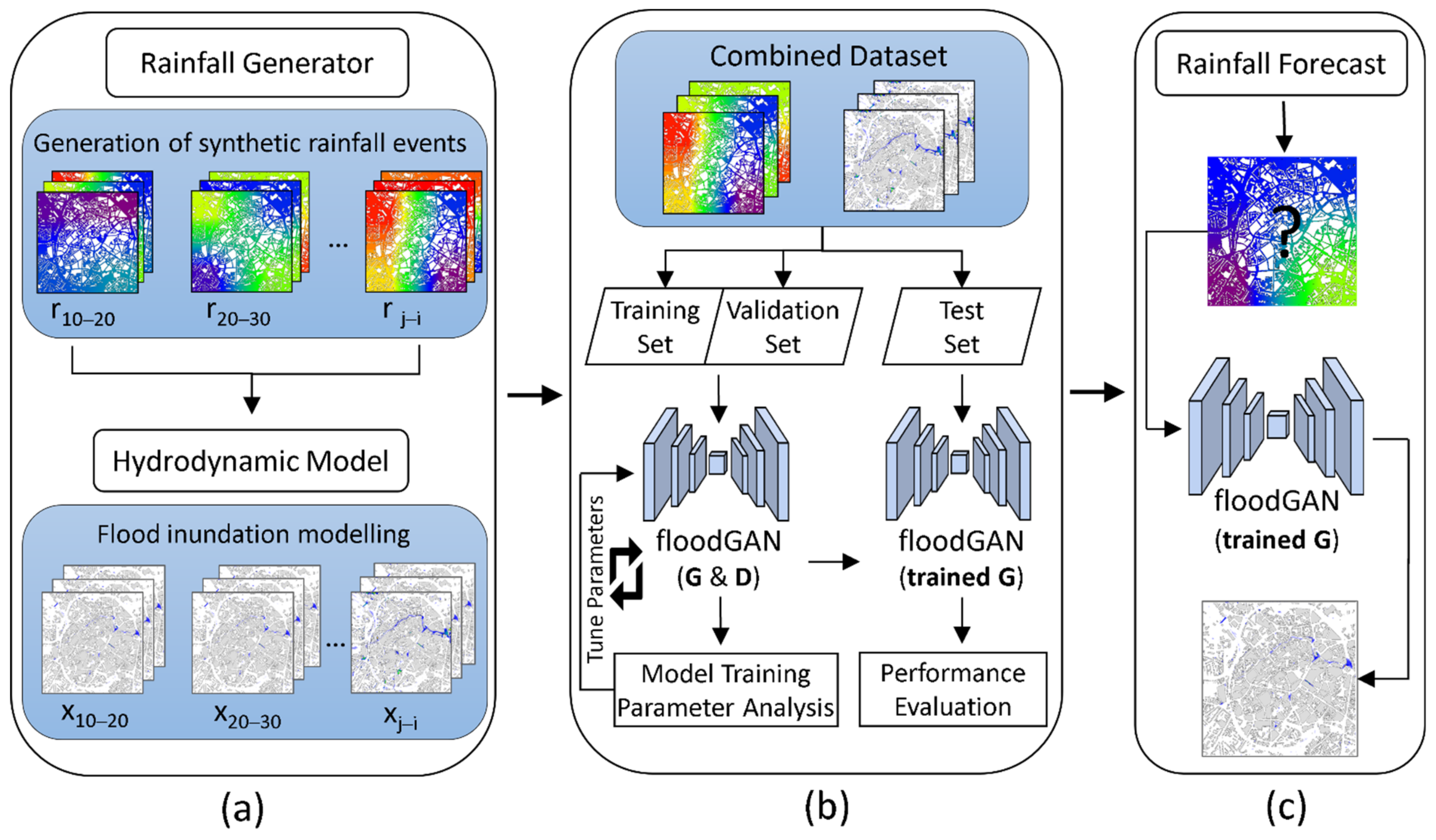
The overall framework of this work is shown in Figure 1. The pipeline consists of three process stages: (a) data generation and preprocessing, (b) offline training, validation and testing, and (c) online prediction.
The first stage generates numerous spatially variable synthetic rainfall events based on a rainfall generator developed. Subsequently, the HD model uses this generated data to simulate the corresponding flooding processes and produce inundation maps. As a result, a combined dataset of rainfall and inundation map is created. To ensure correct translations, an automated, batch-based method is developed and applied to connect numerical values of rainfall intensity and water depth with the channel values of the raster image.
The second stage splits up the combined dataset into training (70%), validation (15%), and test dataset (15%). While the training and validation sets are used to train the floodGAN model and analyze model parameters, the test set serves for the final performance evaluation of the trained floodGAN. During the training process, both the discriminator (D) and the generator (G) are trained and optimized. Consequently, only the trained G is used for the performance evaluation. Ultimately, in the online predictive process, the floodGAN model can predict possible inundations caused by rainfall events that are unfamiliar to the floodGAN model.
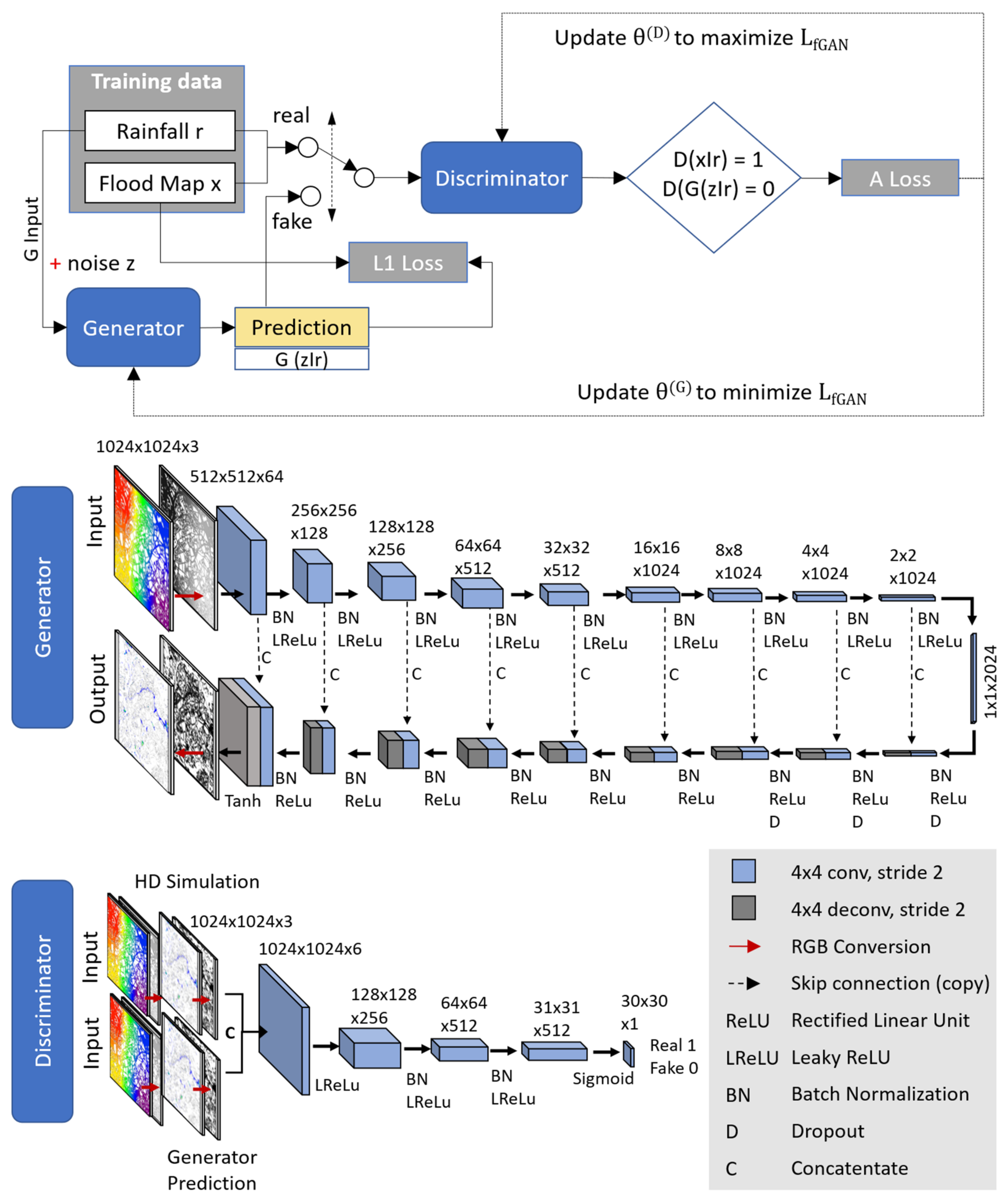
2.4. floodGAN Architecture
The architecture and process workflow of the floodGAN is presented in Figure 2. The discriminator receives input on rainfall and flood maps from the training dataset within the training process, while the generator only receives the rainfall input. The discriminator is trained to label real flood maps x as 1 and the generated flood maps G(z|r) as 0. While the discriminator performs well, the loss function LfGAN has a high value (maximization loss of the discriminator). Similarly, if the generator performs well, the discriminator labels G(z|r) to 1 minimizing the LfGAN. Ideally, the goal is to train a generator that produces loss values close to 0.5, thus producing plausible flood predictions. The discriminator then becomes unable to distinguish between the real flood maps (HD flood simulations) and the flood predictions from the generator.
Isola et al. [44] found that including a mean absolute error loss function (L1 loss) into the cGAN objective increases the accuracy for image translation tasks. Here, the L1 loss improves the generator by increasing its performance to fool the discriminator, producing flood maps that are similar to the ground truth. Therefore, the L1 loss function was adopted from [44] and is given by the following equation:
where the L1 error measures the difference between generated flood map G(z|r) and the ground truth. Consequently, the final objective function used in this study is:
where λ assigns a regularizing weight for the L1 term and, therefore, represents a hyperparameter for model optimization.
The discriminator is updated directly in a standalone procedure during the training process by minimizing the negative log probability of identifying real and fake flood maps measured by the adversarial loss (A loss) [41]. In contrast, the generator is updated based on both A loss and the L1 loss, which are combined into a composite loss function. While the A loss regularizes the quality of plausible images in the target domain, the L1 loss influences the generator to create plausible translations of the rainfall distribution input. The hyperparameter λ controls the composite loss of L1 and A loss.
Concerning the architecture of the floodGAN model, the implemented generator is inspired by a U-Net [45,46], while the discriminator consists of a PatchGAN [44,47] architecture.
The U-Net architecture was initially invented and first applied for biomedical image segmentation [45]. It comprises an encoder-decoder scheme in which the encoder progressively downscales the input image over a few layers until a bottleneck layer using convolutional layers and pooling methods. Subsequently, the decoder progressively upscales the resolution using deconvolutional layers and upsampling methods. The U-Net implemented within this work (1024 × 1024 model) contains 10 convolutional layers, 9 deconvolutional layers and several residual blocks. Furthermore, this network makes use of skip connections to link layers in the encoder with corresponding layers in the decoder that have the same sized feature maps [48], whereby the bottleneck layer is circumvented. While the rectified linear activation unit (ReLu) [49] is applied as the activation function for all the layers of the decoder, the Leaky ReLu (LReLu) [50] is used for the encoder part. The LReLu is based on the ReLu but additionally has a small slope for negative values. In this architecture, a slope value of 0.2 was implemented.
Further, batch normalization [51] is applied after every layer, except the first layer of the encoder and the last layer of the decoder. To reduce overfitting, a dropout of the first three layers of the decoder is used. Finally, a hyperbolic tangent activation function (Tanh) [52] is implemented as an activation function to the last layer of the decoder to receive the flood map for the rainfall input.
Based on a rainfall distribution map and a corresponding flood map, the PatchGAN discriminator calculates the probability of whether the flood map is real or fake. To this end, the PatchGAN architecture consists of five convolutional layers to encode the image pair into a feature vector of size 30 × 30 × 1. Subsequently, a Sigmoid activation function [53] is applied to this feature vector to get the final binary output of the discriminator; it results in 0 for fake and 1 for real. In contrast to the U-Net, the PatchGAN network has no pooling layers. A particular feature of the PatchGAN is that it classifies N × N patches (size of the receptive field) of the input image as real or fake rather than the entire image. In convention with other studies, a patch size of 70 × 70 was found to be effective [44,54]. The discriminator runs convolutionally across the image and averages the responses to calculate the final output of the discriminator. Based on the findings of Isola et al. [44] the kernel size was fixed to 4 × 4 and a stride of 2 × 2 is used on all but the last 2 layers of the discriminator. The slope of the LeakyReLU was set to 0.2. The output of the discriminator is a single feature map that can be averaged to a single score of real/fake predictions.
3. Setup of the Numerical Experiment
The objective of the numerical experiment is to investigate the feasibility of using floodGAN for pluvial flood predictions. For this reason, a numerical experiment was implemented to analyze the performance and accuracy of this model.
The framework of floodGAN was implemented using Python 3.8 and TensorFlow 2.1 [37]. Data pre-and post-processing was conducted using Python 3.8 as well as C++ within the software QT 4.13. The training and testing process was conducted on a 12-core AMD processor (Insitute of Hydraulic Engineering and Water Resources Management, Aachen, Germany) TITAN RTX, with 56 GB-Ram and 68 GB RAM, at the Institute of Hydraulic Engineering and Water Resources Management in Aachen, Germany. Both the simulation of the HD models and the training of the floodGAN model were performed using the graphics card processing unit (GPU). GPUs achieve high performance through parallelism and are optimized for performing pixel computations, processing multiple grid cells or pixels simultaneously.
3.1. Study Area
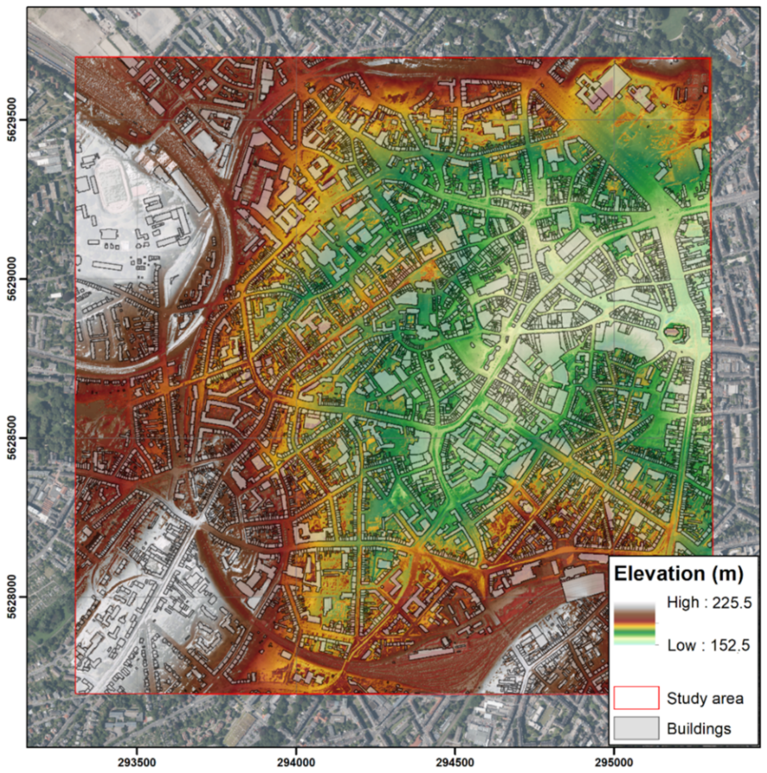
For the implementation of the floodGAN model, a study area in Aachen, Germany, was selected. The study area covers 2 × 2 km2 of the city center and is highly urbanized (Figure 3). It is located in a valley basin, with elevations ranging from 152.5 m to 225.5 m. Due to this topographical situation, the inner city is prone to urban flooding caused by heavy rainfall events. The urban drainage system of the city is designed on rainfall events with return periods between 2 and 5 years. In this study, the capability of the drainage network was assumed to be 20 mm for 1h rainfall events, which is equal to a return period of 2 years.
In the past, the city experienced intense storm events accompanied by urban flooding. on 29 May 2018, Aachen was hit by an extreme convective storm event with short and local but highly intensive rainfall which caused fast surface runoff and urban flooding in the city center. The radar-based and gauge-adjusted quantitative precipitation estimates (QPE) of the RADOLAN (product of the German weather forecast DWD, Offenbach, Germany) [55] and the HydroMaster (product of KISTERS AG, Aachen, Germany) [56] indicated a total amount of rainfall of 40 to 50 mm within 55 minutes. Within the study area, it resulted in an average rainfall intensity of 45 mm/h.
High-resolution quantitative rainfall forecasts (QPF) are provided through the RADVOR product of the DWD as well as the HydroMaster product. Both are provided with a spatial resolution of 1 × 1 km2 and an update rate of 5 minutes. The forecast data is available in the image format ‘GeoTIFF’ via the opendata server of the DWD.
3.2. Datasets
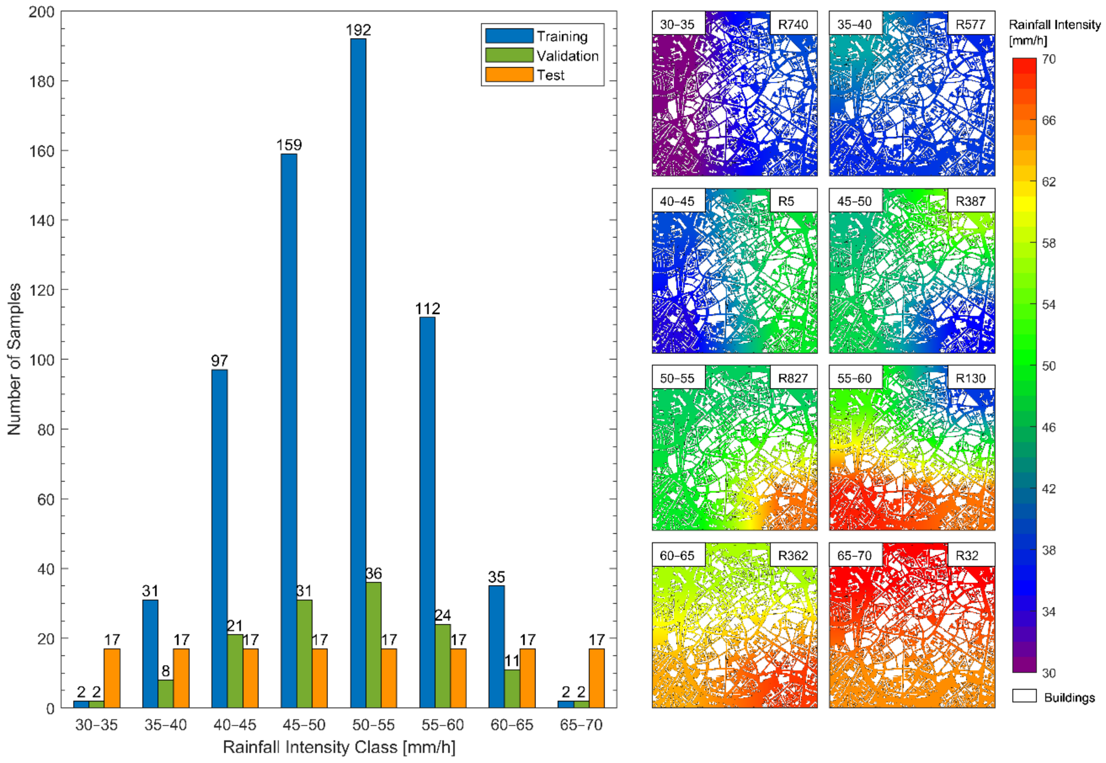
In total, 901 synthetic rainfall events were generated based on the developed rainfall generator. This generator randomly generates rainfall distributions with intensities between 30 and 70 mm/h corresponding to return periods of from 30 to significantly more than 100 years. For example, the intensity belonging to a return period of a 100-year rainfall event for the region of Aachen is at 47 mm/h. The resolution in rainfall intensity was selected with 1mm/h, while the precipitation fields had a spatial range of 200–1000 m.
The events were grouped into 8 classes of 5 mm/h steps and subsequently randomly labeled as training, validation, and test sets comprising 630, 135, and 136 samples. An overview of the distribution of the training, validation, and test datasets is given in Figure 4. While the training and validation data were approximately normally distributed (Gaussian distribution), the test dataset was chosen to be equally distributed. The idea was to investigate the capability to generalize the floodGAN model. Therefore, the model was trained with only a small sample amount of very low and very high intensities, but it was tested with an equal number of low- and high-intensity sample values.
3.3. Hydrodynamic Simulation
Hydrodynamic simulations were carried out to generate inundation maps for corresponding rainfall distributions. The simulations were performed using MIKE 21 Flow Model (MIKE 21 FM) [57]. MIKE 21 FM is a physically based model approach for simulating unsteady free-surface flow processes in coastal and urban areas. The hydrodynamic module is based on the depth-integrated incompressible Reynolds averaged Navier-stokes equation, also known as 2D shallow water equations. To perform the spatial discretization of the 2D shallow water equations, MIKE 21 FM uses a finite volume method and a flexible mesh (FM) method [57].
In this study, the hydrodynamic simulations were conducted using the FM method with a maximum element size of 2 m2 and a minimum time step of 0.01 s. The shallow water equations were solved using a lower-order scheme (first-order) to reduce computational time.
Furthermore, the effect of the drainage system was considered in a generalized approach by a standardized deduction of the total rainfall amount by the capacity (return period) of the urban drainage system, i.e., 20 mm/h (cf. Section 3.1).
The total simulation time was chosen to 3 h, consisting of 1 h rainfall and 2 h follow-up time. Pre-studies have shown that the maximum inundation for 1hr was reached within 2 h runoff time for this specific catchment. Therefore, the calculated inundation maps represented the maximum flood extent and water depth over the entire simulation time.
3.4. Pre-Processing of Raster Images
To enable better training and testing results, the data pairs were converted into uniform-coded images aiming at translations between hydraulic parameters (rainfall intensity and flood depth) and image channels. Therefore, the image channel value of the flood inundation was selected to RGB = 220, 220, 220 (lower bound) and RGB = 20, 20, 20 for higher bound. The same pattern was A spectrum of 120 intervals was chosen for the rainfall images. These processing steps such as reshaping and merging the images, were conducted using C++ and QT.
3.5. Hyperparameters
The floodGAN model contains several hyperparameters that define the network architecture and training scheme, determining the model performance. Here, the essential hyperparameters are the number of epochs, the batch size, the learning rates of discriminator and generator, and the regularizing weight lambda λ.
The number of epochs defines the number of complete passes of model through the training dataset. The internal model parameters of the generator and the discriminator are updated after each epoch. Since the model cannot handle the entire dataset at once, the dataset must be split up into parts (batches). Consequently, the number of batches defines the number of samples that are passed to the model within one epoch. As mentioned in 2.4, lambda controls the weighting of the L1 loss in relation to the adversarial loss.
As default, the floodGAN network was configured with a batch size of 1 constant learning rates of 2 × 10⁴ using an ADAM optimizer with β = 0.5. According to research studies [58], the default value of lambda (λ) was set to 100.
3.6. Performance Assessment
The primary objective of the performance assessment is to investigate the capability of the floodGAN model to emulate the outputs of the 2D HD model. Therefore, the floodGAN results are compared pixel-wise to the HD model in terms of accuracy, precision, computational time, and generalization. In this context, several assessment metrices are adopted to quantify the prediction errors at pixel/cell level.
To assess the quality of the inundation depth predictions of the floodGAN model the Squared Correlation coefficient (R2) and the root mean squared error (RMSE) are provided. The calculation formulas are given below:
where N denotes the number of cells/pixels and Si and Ei denote the flood depth or velocity of simulation and emulation, respectively. The lower the RMSE and the higher the R2 value, the better the agreement between HD simulation and floodGAN prediction.
To evaluate the accuracy of classifying pixels within the flood extent, the precision, recall and F1 score were used as a performance measure. Precision indicates how often the cells are correctly predicted as flooded by the floodGAN model relative to the total amount of all pixels predicted as flooded. The compliment of precision is false discovery rate (1—precision) that represents the rate of overprediction of the floodGAN model. Recall, also known as hit rate, indicates the proportion of cells correctly classified as flooded in relation to the total number of actual flooded cells. The calculation formulae are defined as follows:
where TP denotes the number of true positives (sum of cells correctly predicted as flooded), FP represents the number of false positives (sum of cells incorrectly predicted as flooded). In contrast, FN is the number of false negatives (sum of cells incorrectly predicted as not flooded). The F1 score is the harmonic mean of precision and recall and was used as a summary metric and primary measure for model evaluation. Thus, F1 is an overall measure of a model’s accuracy that combines precision and recall. Consequently, high F1 values indicate that the model results have low false positives and low false negatives. Meaning, in the context of early warning systems, that the model correctly identifies real threats and issues no false alarms. These metrices are commonly used for the evaluation of flood prediction models [59].
4. Results
This section evaluates the performance of the floodGAN model in terms of computation speed, training process, accuracy and generalization. To this end, the results of the floodGAN model were compared to the HD simulations.
First, the floodGAN model was evaluated regarding its computational time and training process on the basis of the training and validation dataset. Secondly, the performance of the floodGAN model was analyzed by using several synthetic rainfall events with varying intensities and spatial distributions on the basis of the test dataset. The aim was to investigate the performance of this model detecting the flood/no-flood pixels and calculating inundation depth values. Finally, the model performance was tested and validated based on records of a historic rainfall event in the city of Aachen, comparing the prediction results of the floodGAN model with the recorded in-situ water depth estimations as well as HD simulations. For the comprehensive test and validation process, the 1024 × 1024-pixel model was used.
4.1. Computational Time and Training Process
As the primary motivation for developing the floodGAN model stems from the need to realize real-time prediction, Table 1 provides the average runtimes of the floodGAN model compared to the HD model. For a spatial resolution of 2 m × 2 m (1024 × 1024 pixel), the HD model required 161 minutes, whereas the floodGAN model only required 0.014 seconds; for a resolution of 1 m × 1 m (2048 × 2048 pixel), the HD-model required 424 minutes, whereas the floodGAN model only required 0.019 seconds, respectively. Consequently, a trained floodGAN model possesses a speed-up factor in the order of 106 and can therefore be used for real-time applications such as early warning systems. Furthermore, the model framework can also be used for larger study areas or numerous ensemble predictions by processing large datasets of various nowcasting products.
The computational time of the HD model varies greatly depending on hydronumerical parameters such as drying and flooding depth or spatial and temporal discretization. In contrast, the prediction time of the floodGAN model is stable and varies slightly regarding the spatial resolution or, relatively, the pixel size.
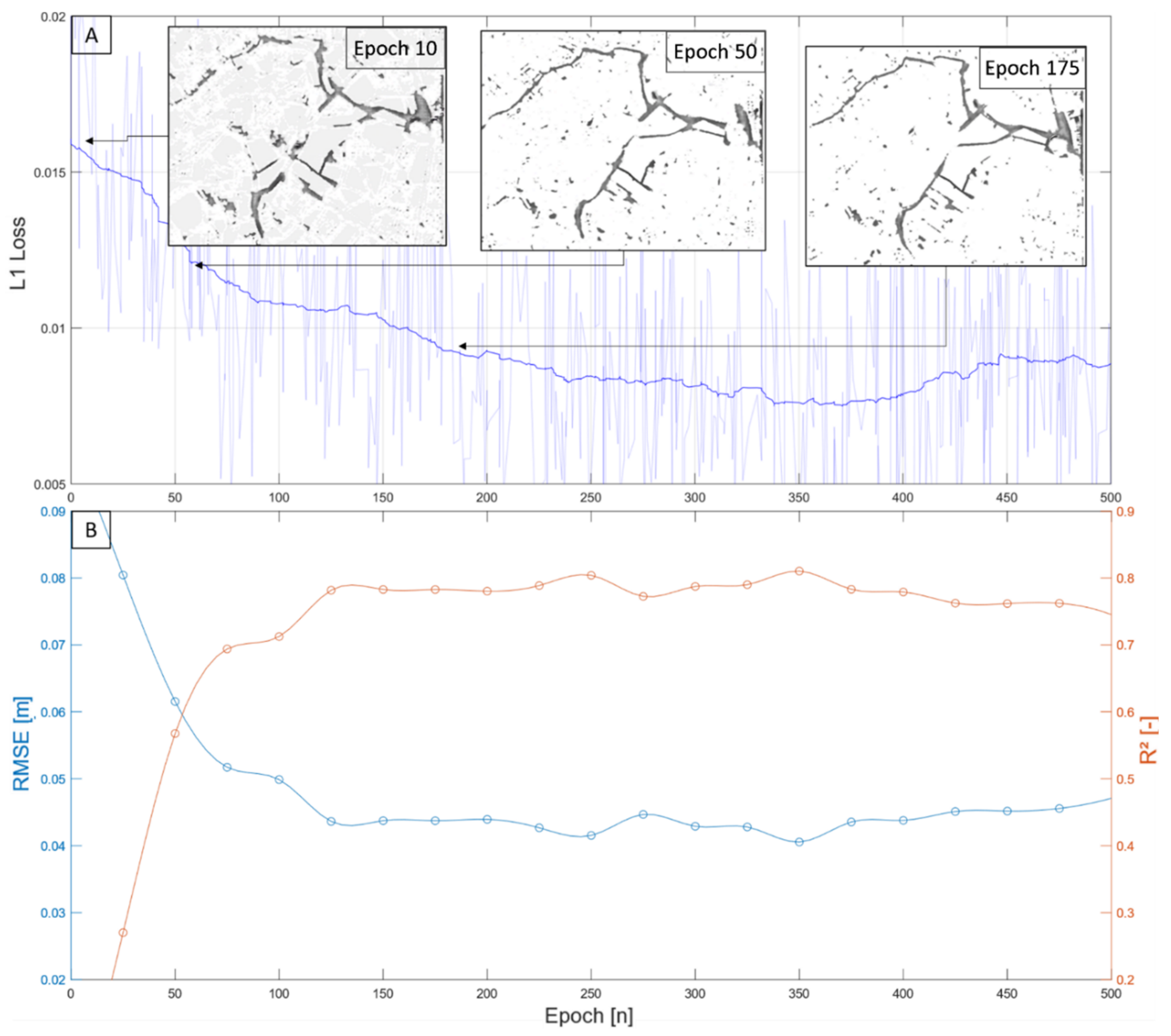
Figure 5A shows a convergence plot of the training process of the 1024 × 1024 floodGAN model, with training epoch on the x-axis and the L1 loss on the y axis (plot above). The L1 loss can be measured directly during the training and is a good indicator for tracking the model performance. The superimposed images show clearly how the prediction quality increases along with the training epochs.
To properly reflect the L1 measure and further evaluate the training process, the mean RMSE and R2 were calculated based on the validation dataset. The evaluation was carried out in 25 epoch steps by comparing the water depth of the predictions with the ones resulting from the simulations based on the validation dataset (Figure 5B). The accuracy of the floodGAN model strongly increased until epoch 125 and reached the first peak at epoch 250. From this point on, the course of R2 and RMSE were relatively stable and reached the optimum accuracy at epoch 350. Subsequently, both plots show a slight trend indicating a deterioration in model quality. This effect can be explained by (a) an overfitting problem or (b) general training difficulties of GAN models, which can be caused by common challenges like catastrophic forgetting [60], oscillations, or model instabilities [61]. Consequently, the discriminator loses its ability to remember synthesized data samples from previous instantiations of the generator.
4.2. Performance Accuracy Assessment
To measure the performance accuracy of the floodGAN model, the different evaluation metrices, namely RMSE, R2, precision, recall and F1 score, were calculated and compared on the basis of the model running for 350 epochs. For a more differentiated assessment regarding different rainfall intensities, the datasets were classified in the four rainfall classes, described in Section 3.
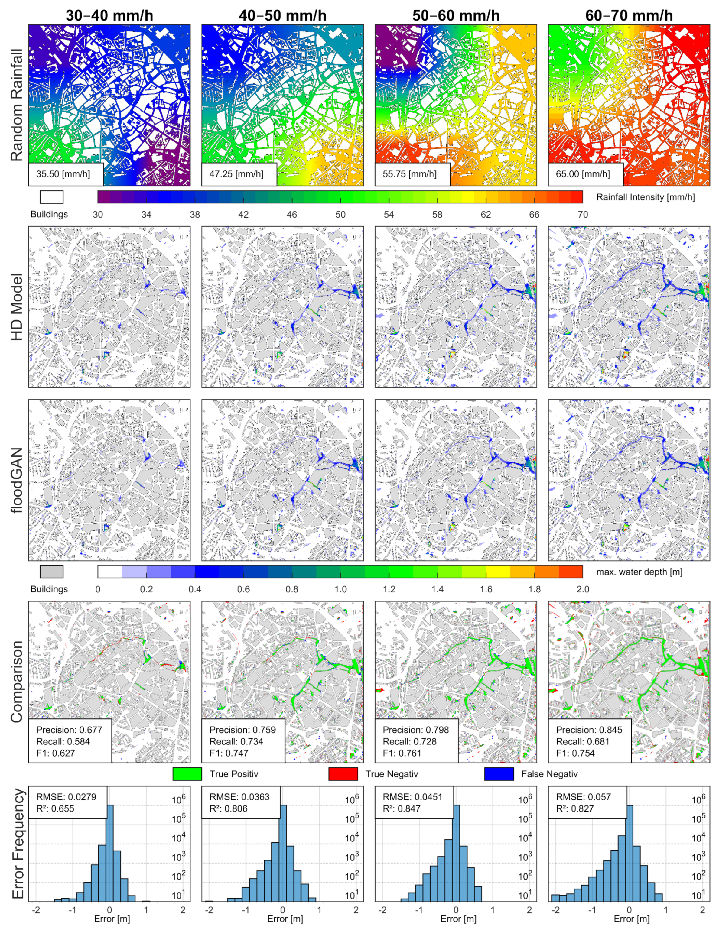
Figure 6 presents the 2D comparison results of four rainfall classes (30–40, 40–50, 50–60, and 60–70 mm/h) randomly selected from the test dataset according to their intensity class. They related to the 8 rainfall classes and were merged in terms of better evaluation capability. Overall, the results demonstrate good prediction accuracies of the floodGAN model for highly variable rainfall intensities and spatially distributed rainfall events. The predictions compare well with the HD-based simulations in terms of flood extent and flood depth. The inundation classification results demonstrated that the floodGAN model detects all relevant flood areas (true positives), with only slight deviations and a small proportion of incorrect predictions (true negatives and false negatives). However, the comparison results indicate higher precision values than recall, indicating an underprediction trend of the floodGAN model. In comparison, the synthetic rainfall scenario of 50–60 mm/h showed the best results with a mean R2 of 0.85 and an RMSE of 0.045 m; it is also characterized by high precision and recall and an F1 score of 0.77. On the other hand, the prediction results of the 30–40 mm/h sample indicated much lower accuracy results.
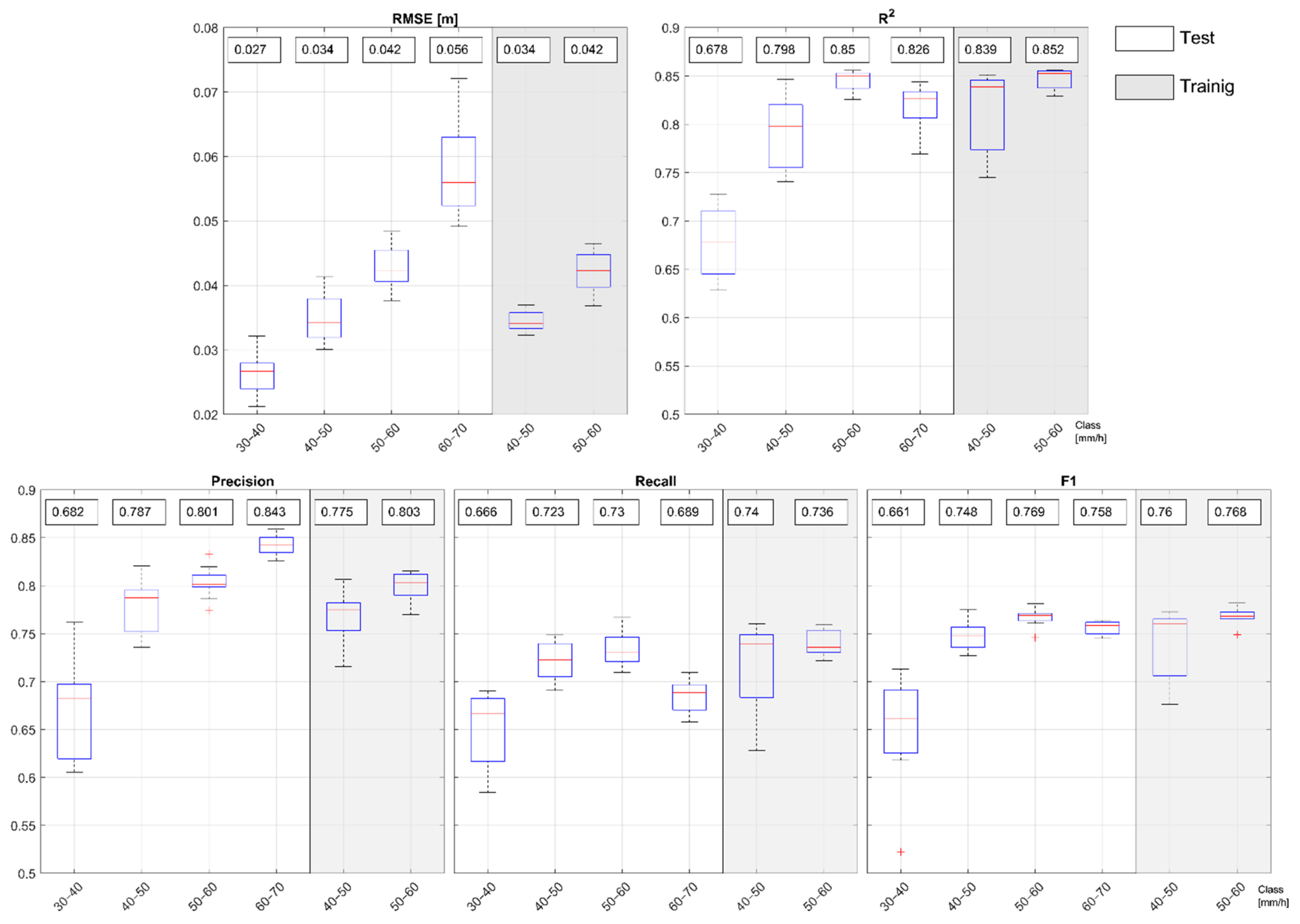
For further analysis and full performance assessment of the floodGAN model, a spectrum of 160 test and training datasets was evaluated. The results are summarized in Figure 7 in which box plots are illustrated for the test datasets across all four rainfall classes. Additionally, the results for two selected rainfall classes of the training dataset are shown in grey. The analysis confirms the high accuracy of class 50–60 mm/h. This can be attributed to (a) a larger amount of training data for this class (cf. Section 3) and (b) transferable information from rainfall intensity patterns from overlapping classes. The evaluation of the boxplots also confirms the low-performance results of class 30–40 mm/h, which in turn can be traced back to the small number of training samples with low rainfall intensities and spatial patterns.
R2 scores higher than 0.8 demonstrate a good correlation regarding the inundation depth values. Furthermore, the mean RMSE value increases with rainfall intensities and, therefore, the water depth. Consequently, the lowest RMSE values are connected to low rainfall intensities because the total water amount is lower. Overall, the results confirm the trend of having higher precision than recall, indicating more false negatives (incorrectly predicting a pixel as non-flooded) than false positives (incorrectly predicting a pixel as flooded). Therefore, the floodGAN model generally underpredicts the inundation extent.
Moreover, the prediction results of the training datasets do not show much higher performance values than those from the test datasets, suggesting that the floodGAN model generalizes well with different rainfall distributions. This can be confirmed by considering the good prediction results of non-existing combinations of rainfall patterns in the training data, which are thus “unfamiliar” to the floodGAN. Consequently, it can be concluded that the model can manage new and arbitrary rainfall distributions.
4.3. Setup 2: Validation on Historic Pluvial Flood Event
Finally, the floodGAN model was tested and validated regarding the prediction of maximum inundation extent and water depth of the historic pluvial flood event on 29th of May 2018 in Aachen. Figure 8 presents the comparison between the simulation of the HD model and the prediction of floodGAN against the in-situ recordings of the event. It can be seen that the floodGAN predictions generally demonstrate a very high agreement with the simulated inundation maps in terms of water depth values and inundation extent. All flood hotspots are covered well by the floodGAN model. Only small parts of the inundation extend are not detected in the prediction, which means that the floodGAN model underestimates the flood extent resulting in higher precision than recall leading to an F1 score of 0.78 to 0.79. The absolute errors between HD simulation and floodGAN prediction were between −0.1 to −0.2 m in mainly flooded areas while higher differences of −0.80 m and +0.50 m occasionally appeared close to the model boundaries. This effect indicated that boundary effects should be critically examined. The RMSE calculated resulted in 0.035 m.
To further validate the floodGAN performance against the real flood event, in-situ observations were used to compare the HD simulation to the floodGAN predictions. Table 2 shows the results of predictions and simulations in relation to the in-situ estimated flood depths compared at four locations. The deviations between simulations and predictions appear to be very small compared to the difference to in-situ observations. Thus, in the context of early warning systems, the predictions of the floodGAN model are precise enough for application in operational systems.
5. Discussion
In the context of operational flood prediction systems, the choice of modelling methods is essentially driven by conflicting priorities of accuracy, computation speed, data needs and practical implementation. Therefore, the floodGAN model proposed is discussed along the same lines.
The performance tests have demonstrated that the inundation predictions of the floodGAN model compare well with the results of the HD simulations regarding the flood extent and water depth. The predictions are accurate for unknown spatially distributed rainfall events, proving the high generalizability of the proposed deep learning model. Mean R2 values of the conducted test datasets range from 0.80 to 0.85 and mean F1 scores range between 0.75 and 0.77, while low values can be attributed to the insufficient amount of training data covering low rainfall intensities. The study examines how many training samples are needed for good model performances by analyzing the class-specific results compared to the number of training samples. As the samples are categorized by rainfall intensities of 10 mm/h, the authors suggest that 70–100 training samples are needed to achieve satisfactory results. Validation tests on a historic rainfall event have shown that the accuracy achieved is sufficient for operational purposes since HD models themselves involve uncertainties connected to their assumptions and simplifications.
The computational runtime of the floodGAN model is more than convincing. This model calculates flood predictions 106 times faster than an HD model, enabling real-time projections of large areas and several predictions with varying rainfall inputs. Ideally, robust prediction is based on numerous model runs that cover different ensembles of rainfall forecasts to produce probabilistic flood hazard maps. In this context, compared to other data-driven models, the main advantage of floodGAN is the effective use of CNNs to process spatially related rainfall-flood data and handle high-resolution inputs without facing exponential growth of computational time. Further, using the image-to-image translation approach provides an effective technique for end-to-end early warning systems by direct predictions of inundations immediately derived from raw rainfall inputs like radar-based nowcasts. Another significant benefit of using GANs is their capability of learning large and complex data distributions with a relatively small number of parameters. Unlike discriminative models like ANNs, GANs can learn the relevant features from large and even unlabeled datasets—a process that requires little to no labeling or human supervision.
However, despite the promising performance results and advantages of the floodGAN model, several challenges and drawbacks remain and require further investigations. These challenges can be divided into algorithm- and framework-related issues.
A major challenge of using GANs for flood prediction tasks is connected to their training difficulties which arise when data generating distribution becomes more complex. During this work it has been noticed that improving the performance of the floodGAN can be elusive. Due to the simultaneous training of the generator and discriminator, difficulty arises when trying to realize the convergence of generator and discriminator to improve the GAN model’s performance [42]. During the testing process of different model parameter setups, either the discriminator or generator became too strong, resulting in the collapse of the entire model. Recent studies demonstrate that the use of multiple generators and discriminators and their simultaneous training can lead to improved convergence and better results [62]. This approach was proposed by J-Y. Zhu et al. [63] and consists of a cycle where the generated translation is looped back into again into the process of the generator.
In terms of practicability, the execution of hydrodynamic simulations to generate the train, validation and test datasets required 75 days using an above-average computer system equipped with one GPU. Consequently, the computational duration, and therefore the development of a floodGAN model covering larger areas in a high resolution, is very high. The application of parameter optimization techniques [13] to speed up the simulation process combined with multiple GPUs [64] or distributed computing [65,66] could likely allow the large-scale application of this method, which is a planned future direction of research activities.
Furthermore, a significant challenge belongs to the transferability and scalability of the model. In its current implementation, the floodGAN model is generalized on spatially variable rainfall inputs in one specific catchment. Consequently, the developed model is domain-specific and therefore can be used only for one area. As a further result, significant hydraulic changes in the urban infrastructure would require a complete re-training of the floodGAN model. Given this drawback, the framework’s modifications that include terrain surface information within the training process are necessary. One solution could be implementing topographic features such as elevation, aspect, slope, and curvature within additional image channels [24]. This modified framework would allow the floodGAN model to be trained for one area but to be also transferable and applicable in different areas.
Further, floodGAN allows the prediction of inundation solely on a single driver, i.e., rainfall. However, the method can be adapted to predict flooding processes from different drivers, e.g., compound flooding in urban coastal areas. To achieve this, it is necessary to enhance the framework in several ways to consider the compound effect of storm surge and rainfall. First, the hydrodynamic model needs to be adjusted to model the interaction processes of pluvial and coastal flooding based on a coupled ocean and urban flood model. Secondly, numerous different scenarios must be generated to describe possible superimpositions of both flood drivers. Finally, the floodGAN model is trained on the basis of the HD output data. It remains a research question to cover long flood durations and large combinations due to the high computational costs needed to generate the training data.
Another limitation of the current floodGAN model relates to the prediction of the temporal dynamics of the flooding processes. This issue could be solved by dynamic extraction and training with latent representations of the rainfall and flooding processes. Therefore, the current floodGAN framework must be enhanced using RNN, for example LSTM algorithms, to capture the temporal dynamics. Recent studies from the medical sector have demonstrated that RNNs can be implemented into the discriminator and generator of conditional GANs (recurrent CGAN) to predict multidimensional time series [67]. Furthermore, the current framework does not include other hydraulic parameters such as flow velocity. These can be taken into account by implementing relevant data into additional image channels.
6. Conclusions
In this work, a deep learning model has been proposed to predict 2D flood inundations caused by spatially highly variable rainfall events. A key factor in the model development was searching for the fastest and most straightforward solution for an end-to-end flood prediction method while maintaining a high model accuracy. As a result, unlike other data-driven models, the floodGAN model proposed takes a shortcut by directly translating flood hazard maps from raw rainfall images based on an image-to-image translation approach. This method accelerates the computation speed of detailed flood predictions tremendously and thus overcomes the computational bottleneck of performing high-resolution flood simulations using HD models.
The floodGAN model was trained and tested based on a case study of Aachen using synthetic as well as real rainfall events and showed promising results in terms of accuracy and computational cost. The vast speed gain combined the low loss of accuracy highlights the high potential of the floodGAN model for real-time applications as required for early warning, real-time control of urban drainage systems, or the generation of numerous probabilistic flood hazard maps using ensemble forecasts. For this purpose, the model was specially designed to work with (a) high-dimensional input data and (b) highly detailed rainfall forecasts that are, or in the near future will be, widely available. Further, the pipeline can be potentially transferred to similar event-related 2D prediction problems.
As a main drawback, the present study only focused on predicting maximum inundation extent and water depth for up to 1hr rainfall events and does not include the prediction of flow velocities. Furthermore, although the floodGAN model can generate current inundation maps for each updated precipitation forecast. However, it does not take the serial correlation of time series data of flooding into account. Consequently, the current model neglects the temporal dynamics of flooding processes, and the prediction results are limited to quasi-static flood hazard maps.
Future work will focus on overcoming this limitation by (1) implementing RNN or LSTM algorithms into the floodGAN model and (2) training the model with time series of hydrodynamic-based flood simulations. The aim will be to develop a dynamic floodGAN which can predict time-related flooding processes to capture the timing to inundation peak and the flood duration. Concomitantly, the performance of the floodGAN model will be improved by testing different loss functions and implementing multiple generators and discriminators into the model architecture.
Furthermore, the model generalization’s and transferability as well as the prediction capability of additional hydraulic parameters will be tested by increasing the number of channels and features of the training datasets. Another important goal is to investigate the scalability of the developed approach. However, the generation of the required training datasets is still connected to high computational costs at the current state. This goal can be envisaged using parallel high-performance computing and distributed systems. Finally, it would be exciting to extend the current floodGAN architecture by implementing algorithms of RNNs aiming at developing a dynamic prediction model to describe time-related flooding processes.
Author Contributions
Conceptualization, J.H.; Methodology, J.H.; Modelling, J.H.; Formal Analysis, J.H.; Resources, J.H. and H.S.; Data Curation, J.H.; Writing—Original Draft, J.H.; Writing—Review and Editing, J.H. and H.S.; Visualization, J.H.; Supervision, H.S. All authors have read and agreed to the published version of the manuscript.
Funding
This research received no external funding.
Acknowledgments
The authors thank DHI for providing the Software MIKE 21/MIKE Flood.
Conflicts of Interest
The authors declare no conflict of interest.
References
- René, J.-R.; Djordjević, S.; Butler, D.; Madsen, H.; Mark, O. Assessing the potential for real-time urban flood forecasting based on a worldwide survey on data availability. Urban Water J. 2014, 11, 573–583. [Google Scholar] [CrossRef] [Green Version]
- Borga, M.; Anagnostou, E.N.; Blöschl, G.; Creutin, J.-D. Flash flood forecasting, warning and risk management: The HYDRATE project. Environ. Sci. Policy 2011, 14, 834–844. [Google Scholar] [CrossRef]
- WMO. Flash Flood Forecasting: WMO-No.577, Switzerland. Available online: https://library.wmo.int/pmb_ged/wmo_577.pdf (accessed on 2 February 2021).
- Foresti, L.; Seed, A. On the spatial distribution of rainfall nowcasting errors due to orographic forcing. Meteorol. Appl. 2015, 22, 60–74. [Google Scholar] [CrossRef]
- Schumacher, R.S. Heavy Rainfall and Flash Flooding. In Oxford Research Encyclopedias; Cutter, S.L., Ed.; Oxford University Press: Oxford, UK, 2016; ISBN 9780199389407. [Google Scholar]
- Jasper-Tönnies, A.; Hellmers, S.; Einfalt, T.; Strehz, A.; Fröhle, P. Ensembles of radar nowcasts and COSMO-DE-EPS for urban flood management. Water Sci. Technol. 2017, 2017, 27–35. [Google Scholar] [CrossRef]
- Zanchetta, A.D.L.; Coulibaly, P. Recent Advances in Real-Time Pluvial Flash Flood Forecasting. Water 2020, 12, 570. [Google Scholar] [CrossRef] [Green Version]
- Henonin, J.; Russo, B.; Mark, O.; Gourbesville, P. Real-time urban flood forecasting and modelling—A state of the art. J. Hydroinform. 2013, 15, 717–736. [Google Scholar] [CrossRef]
- Leandro, J.; Schumann, A.; Pfister, A. A step towards considering the spatial heterogeneity of urban key features in urban hydrology flood modelling. J. Hydrol. 2016, 535, 356–365. [Google Scholar] [CrossRef]
- Bates, P.D.; Horritt, M.S.; Fewtrell, T.J. A simple inertial formulation of the shallow water equations for efficient two-dimensional flood inundation modelling. J. Hydrol. 2010, 387, 33–45. [Google Scholar] [CrossRef]
- De Almeida, G.A.M.; Bates, P.; Freer, J.E.; Souvignet, M. Improving the stability of a simple formulation of the shallow water equations for 2-D flood modeling. Water Resour. Res. 2012, 48, W05528. [Google Scholar] [CrossRef]
- Courty, L.G.; Pedrozo-Acuña, A.; Bates, P.D. Itzï (version 17.1): An open-source, distributed GIS model for dynamic flood simulation. Geosci. Model Dev. 2017, 10, 1835–1847. [Google Scholar] [CrossRef] [Green Version]
- Hofmann, J.; Schüttrumpf, H. Risk-Based and Hydrodynamic Pluvial Flood Forecasts in Real Time. Water 2020, 12, 1895. [Google Scholar] [CrossRef]
- Leandro, J.; Chen, A.S.; Djordjević, S.; Savić, D.A. Comparison of 1D/1D and 1D/2D Coupled (Sewer/Surface) Hydraulic Models for Urban Flood Simulation. J. Hydraul. Eng. 2009, 135, 495–504. [Google Scholar] [CrossRef]
- Fan, Y.; Ao, T.; Yu, H.; Huang, G.; Li, X. A Coupled 1D-2D Hydrodynamic Model for Urban Flood Inundation. Adv. Meteorol. 2017, 2017, 1–12. [Google Scholar] [CrossRef] [Green Version]
- Shen, C. A Transdisciplinary Review of Deep Learning Research and Its Relevance for Water Resources Scientists. Water Resour. Res. 2018, 54, 8558–8593. [Google Scholar] [CrossRef]
- Chang, F.-J.; Hsu, K.; Chang, L.-C. Flood Forecasting Using Machine Learning Methods; MDPI AG: Basel, Switzerland, 2019; ISBN 3038975486. [Google Scholar]
- Chu, H.; Wu, W.; Wang, Q.J.; Nathan, R.; Wei, J. An ANN-based emulation modelling framework for flood inundation modelling: Application, challenges and future directions. Environ. Model. Softw. 2020, 124, 104587. [Google Scholar] [CrossRef]
- Lin, Q.; Leandro, J.; Gerber, S.; Disse, M. Multistep Flood Inundation Forecasts with Resilient Backpropagation Neural Networks: Kulmbach Case Study. Water 2020, 12, 3568. [Google Scholar] [CrossRef]
- Tealab, A. Time series forecasting using artificial neural networks methodologies: A systematic review. Future Comput. Inform. J. 2018, 3, 334–340. [Google Scholar] [CrossRef]
- Kim, H.I.; Han, K.Y. Urban Flood Prediction Using Deep Neural Network with Data Augmentation. Water 2020, 12, 899. [Google Scholar] [CrossRef] [Green Version]
- Tien Bui, D.; Hoang, N.-D.; Martínez-Álvarez, F.; Ngo, P.-T.T.; Hoa, P.V.; Pham, T.D.; Samui, P.; Costache, R. A novel deep learning neural network approach for predicting flash flood susceptibility: A case study at a high frequency tropical storm area. Sci. Total Environ. 2020, 701, 134413. [Google Scholar] [CrossRef] [PubMed]
- Berkhahn, S.; Fuchs, L.; Neuweiler, I. An ensemble neural network model for real-time prediction of urban floods. J. Hydrol. 2019, 575, 743–754. [Google Scholar] [CrossRef]
- Guo, Z.; Leitão, J.P.; Simões, N.E.; Moosavi, V. Data-driven flood emulation: Speeding up urban flood predictions by deep convolutional neural networks. J. Flood Risk Manag. 2021, 14, e12684. [Google Scholar] [CrossRef]
- LeCun, Y.; Bengio, Y.; Hinton, G. Deep learning. Nature 2015, 521, 436–444. [Google Scholar] [CrossRef]
- Moy de Vitry, M.; Kramer, S.; Wegner, J.D.; Leitão, J.P. Scalable flood level trend monitoring with surveillance cameras using a deep convolutional neural network. Hydrol. Earth Syst. Sci. 2019, 23, 4621–4634. [Google Scholar] [CrossRef] [Green Version]
- Wang, Y.; Fang, Z.; Hong, H.; Peng, L. Flood susceptibility mapping using convolutional neural network frameworks. J. Hydrol. 2020, 582, 124482. [Google Scholar] [CrossRef]
- Kabir, S.; Patidar, S.; Xia, X.; Liang, Q.; Neal, J.; Pender, G. A deep convolutional neural network model for rapid prediction of fluvial flood inundation. J. Hydrol. 2020, 590, 125481. [Google Scholar] [CrossRef]
- Zhou, Y.; Wu, W.; Nathan, R.; Wang, Q.J. A rapid flood inundation modelling framework using deep learning with spatial reduction and reconstruction. Environ. Model. Softw. 2021, 143, 105112. [Google Scholar] [CrossRef]
- Creswell, A.; White, T.; Dumoulin, V.; Arulkumaran, K.; Sengupta, B.; Bharath, A.A. Generative Adversarial Networks: An Overview. IEEE Signal Process. Mag. 2018, 35, 53–65. [Google Scholar] [CrossRef] [Green Version]
- Ledig, C.; Theis, L.; Huszar, F.; Caballero, J.; Cunningham, A.; Acosta, A.; Aitken, A.; Tejani, A.; Totz, J.; Wang, Z.; et al. Photo-Realistic Single Image Super-Resolution Using a Generative Adversarial Network. In Proceedings of the 30th IEEE Conference on Computer Vision and Pattern Recognition, Honolulu, HI, USA, 21–26 July 2016. [Google Scholar]
- Kaji, S.; Kida, S. Overview of image-to-image translation by use of deep neural networks: Denoising, super-resolution, modality conversion, and reconstruction in medical imaging. Radiol. Phys. Technol. 2019, 12, 235–248. [Google Scholar] [CrossRef] [Green Version]
- Lin, S.; Qin, F.; Li, Y.; Bly, R.A.; Moe, K.S.; Hannaford, B. LC-GAN: Image-to-Image Translation Based on Generative Adversarial Network for Endoscopic Images. 2020. Available online: https://arxiv.org/pdf/2003.04949 (accessed on 26 February 2021).
- Luo, J.; Huang, J.; Li, H. A case study of conditional deep convolutional generative adversarial networks in machine fault diagnosis. J. Intell. Manuf. 2021, 32, 407–425. [Google Scholar] [CrossRef]
- Farimani, A.B.; Gomes, J.; Pande, V.S. Deep Learning the Physics of Transport Phenomena. 2017. Available online: https://arxiv.org/pdf/1709.02432 (accessed on 27 February 2021).
- Dagasan, Y.; Juda, P.; Renard, P. Using Generative Adversarial Networks as a Fast Forward Operator for Hydrogeological Inverse Problems. Ground Water 2020, 58, 938–950. [Google Scholar] [CrossRef]
- Cheng, M.; Fang, F.; Pain, C.C.; Navon, I.M. Data-driven modelling of nonlinear spatio-temporal fluid flows using a deep convolutional generative adversarial network. Comput. Methods Appl. Mech. Eng. 2020, 365, 113000. [Google Scholar] [CrossRef] [Green Version]
- Lecun, Y.; Bottou, L.; Bengio, Y.; Haffner, P. Gradient-based learning applied to document recognition. Proc. IEEE 1998, 86, 2278–2324. [Google Scholar] [CrossRef] [Green Version]
- Gu, J.; Wang, Z.; Kuen, J.; Ma, L.; Shahroudy, A.; Shuai, B.; Liu, T.; Wang, X.; Wang, L.; Wang, G.; et al. Recent Advances in Convolutional Neural Networks. 2015. Available online: https://arxiv.org/pdf/1512.07108 (accessed on 27 February 2021).
- Luo, W.; Li, Y.; Urtasun, R.; Zemel, R. Understanding the Effective Receptive Field in Deep Convolutional Neural Networks. 2017. Available online: https://arxiv.org/pdf/1701.04128 (accessed on 27 February 2021).
- Goodfellow, I.J.; Pouget-Abadie, J.; Mirza, M.; Xu, B.; Warde-Farley, D.; Ozair, S.; Courville, A.; Bengio, Y. Generative Adversarial Networks. 2014. Available online: https://arxiv.org/pdf/1406.2661 (accessed on 28 February 2021).
- Radford, A.; Metz, L.; Chintala, S. Unsupervised Representation Learning with Deep Convolutional Generative Adversarial Networks. 2015. Available online: https://arxiv.org/pdf/1511.06434 (accessed on 28 February 2021).
- Mirza, M.; Osindero, S. Conditional Generative Adversarial Nets. 2014. Available online: https://arxiv.org/pdf/1411.1784 (accessed on 2 March 2021).
- Isola, P.; Zhu, J.-Y.; Zhou, T.; Efros, A.A. Image-to-Image Translation with Conditional Adversarial Networks. In Proceedings of the 30th IEEE Conference on Computer Vision and Pattern Recognition (CVPR), Honolulu, HI, USA, 21–26 July 2016. [Google Scholar]
- Ronneberger, O.; Fischer, P.; Brox, T. U-Net: Convolutional Networks for Biomedical Image Segmentation; Springer: Berlin/Heidelberg, Germany, 2015; Available online: http://dx.doi.org/10.1007/978-3-319-24574-4_28 (accessed on 4 March 2021).
- Badrinarayanan, V.; Kendall, A.; Cipolla, R. SegNet: A Deep Convolutional Encoder-Decoder Architecture for Image Segmentation. IEEE Trans. Pattern Anal. Mach. Intell. 2017, 39, 2481–2495. [Google Scholar] [CrossRef] [PubMed]
- Li, C.; Wand, M. Precomputed Real-Time Texture Synthesis with Markovian Generative Adversarial Networks. 2016. Available online: https://arxiv.org/pdf/1604.04382 (accessed on 4 March 2021).
- Srivastava, R.K.; Greff, K.; Schmidhuber, J. Training Very Deep Networks. 2015. Available online: https://arxiv.org/pdf/1507.06228 (accessed on 4 March 2021).
- Nair, V.; Hinton, G.E. Rectified Linear Units Improve Restricted Boltzmann Machines. In Proceedings of the 27th International Conference on Machine Learning, Toronto, ON, Canada, 7–10 January 2010; Available online: https://www.cs.toronto.edu/~fritz/absps/reluICML.pdf (accessed on 4 March 2021).
- Clevert, D.-A.; Unterthiner, T.; Hochreiter, S. Fast and Accurate Deep Network Learning by Exponential Linear Units (ELUs). 2015. Available online: http://arxiv.org/pdf/1511.07289v5 (accessed on 4 March 2021).
- Ioffe, S.; Szegedy, C. Batch Normalization: Accelerating Deep Network Training by Reducing Internal Covariate Shift. 2015. Available online: https://arxiv.org/pdf/1502.03167 (accessed on 5 March 2021).
- LeCun, Y.A.; Bottou, L.; Orr, G.B.; Müller, K.-R. Efficient BackProp. In Neural Networks: Tricks of the Trade, 2nd ed.; Montavon, G., Ed.; Springer: Berlin/Heidelberg, Germany, 2012; pp. 9–48. ISBN 978-3-642-35288-1. [Google Scholar]
- Han, J.; Moraga, C. The influence of the sigmoid function parameters on the speed of backpropagation learning. In From Natural to Artificial Neural Computation: Proceedings; Mira, J., Ed.; Springer: Berlin/Heidelberg, Germany, 1995; pp. 195–201. ISBN 978-3-540-59497-0. [Google Scholar]
- Hamwood, J.; Alonso-Caneiro, D.; Read, S.A.; Vincent, S.J.; Collins, M.J. Effect of patch size and network architecture on a convolutional neural network approach for automatic segmentation of OCT retinal layers. Biomed. Opt. Express 2018, 9, 3049–3066. [Google Scholar] [CrossRef] [PubMed] [Green Version]
- DWD. RADOLAN/RADVOR: Hochaufgelöste Niederschlagsanalyse und-Vorhersage auf der Basis Quantitativer Radar-und Ombrometerdaten für Grenzüberschreitende Fluss-Einzugsgebiete von Deutschland im Echtzeitbetrieb, Offenbach. 2019. Available online: https://www.dwd.de/DE/leistungen/radvor/radvor.html (accessed on 5 March 2021).
- KISTERS AG. Available online: https://www.hydromaster.com/de/ (accessed on 5 March 2021).
- DHI. MIKE 21 Flow Model FM: Hydrodynamic Module, Denmark. 2017. Available online: https://manuals.mikepoweredbydhi.help/2017/Coast_and_Sea/MIKE_FM_HD_2D.pdf (accessed on 5 March 2021).
- Alarsan, F.; Younes, M. Best Selection of Generative Adversarial Networks Hyper-Parameters using Genetic Algorithm. 2020. Available online: https://www.researchsquare.com/article/rs-95571/v1 (accessed on 5 March 2021).
- Aronica, G.; Bates, P.D.; Horritt, M.S. Assessing the uncertainty in distributed model predictions using observed binary pattern information within GLUE. Hydrol. Process. 2002, 16, 2001–2016. [Google Scholar] [CrossRef]
- Thanh-Tung, H.; Tran, T. On Catastrophic Forgetting and Mode Collapse in Generative Adversarial Networks. 2018. Available online: http://arxiv.org/pdf/1807.04015v8 (accessed on 5 March 2021).
- Xu, K.; Li, C.; Zhu, J.; Zhang, B. Understanding and Stabilizing GANs’ Training Dynamics with Control Theory. 2019. Available online: http://arxiv.org/pdf/1909.13188v4 (accessed on 5 March 2021).
- Im Jiwoong, D.; Ma, H.; Kim, C.D.; Taylor, G. Generative Adversarial Parallelization. 2016. Available online: http://arxiv.org/pdf/1612.04021v1 (accessed on 5 March 2021).
- Zhu, J.-Y.; Park, T.; Isola, P.; Efros, A.A. Unpaired Image-to-Image Translation Using Cycle-Consistent Adversarial Networks. In Proceedings of the 2017 IEEE International Conference on Computer Vision (ICCV), Venice, Italy, 22–29 October 2017; IEEE: Piscataway, NJ, USA, 2017; pp. 2242–2251, ISBN 978-1-5386-1032-9. [Google Scholar]
- Xing, Y.; Liang, Q.; Wang, G.; Ming, X.; Xia, X. City-scale hydrodynamic modelling of urban flash floods: The issues of scale and resolution. Nat. Hazards 2019, 96, 473–496. [Google Scholar] [CrossRef] [Green Version]
- Mayer, R.; Jacobsen, H.-A. Scalable Deep Learning on Distributed Infrastructures. ACM Comput. Surv. 2020, 53, 1–37. [Google Scholar] [CrossRef] [Green Version]
- Gonnet, P. Efficient and Scalable Algorithms for Smoothed Particle Hydrodynamics on Hybrid Shared/Distributed-Memory Architectures. SIAM J. Sci. Comput. 2015, 37, C95–C121. [Google Scholar] [CrossRef] [Green Version]
- Esteban, C.; Hyland, S.L.; Rätsch, G. Real-Valued (Medical) Time Series Generation with Recurrent Conditional GANs. 2017. Available online: https://arxiv.org/pdf/1706.02633 (accessed on 5 March 2021).
Figure 1.
Overall framework. (a) The rainfall generator generates synthetic rainfall events and the HD model simulates corresponding flood inundation maps. (b) The data pairs are used to train and test the floodGAN model. (c) The trained floodGAN model can be used for online prediction by coupling it with a rainfall forecasting systems.

Figure 2.
floodGAN architecture and process flow of the training.

Figure 3.
Digital elevation model (DEM) of the study area including building data.

Figure 4.
Distribution of training, validation and test datasets (left) and exemplary rainfall samples (right). Rn represents the number of the sample from the corresponding rainfall intensity class.
Figure 4.
Distribution of training, validation and test datasets (left) and exemplary rainfall samples (right). Rn represents the number of the sample from the corresponding rainfall intensity class.

Figure 5.
L1 loss values (A) and RMSE and R2 (B) calculated for a training of 500 epochs.

Figure 6.
Prediction results of the floodGAN model for different rainfall scenarios compared to the HD simulations.
Figure 6.
Prediction results of the floodGAN model for different rainfall scenarios compared to the HD simulations.

Figure 7.
RMSE, R2, Precision, Recall and F1 for different test and training datasets sorted in rainfall classes.
Figure 7.
RMSE, R2, Precision, Recall and F1 for different test and training datasets sorted in rainfall classes.

Figure 8.
Comparisons of the floodGAN model and the HD model with in-situ recordings for the pluvial flood event on 29 May 2018 in Aachen. Panels A and B show HD simulation and floodGAN prediction, while panels C and D present the comparison and water depth. Photos 1–4 highlight flooded areas in the city of Aachen and are located in panel A.


Table 1.
Average runtime performance of the floodGAN model for an average training rate of 350 epochs compared to HD simulations.
Table 1.
Average runtime performance of the floodGAN model for an average training rate of 350 epochs compared to HD simulations.
| Model Size (Pixel) | Grid Resolution (m) | Training Time (h) | Prediction Time (s) | HD Simulation (min) * | Speed-Up Ratio (-) |
|---|---|---|---|---|---|
| 128 × 128 | 16 × 16 | 1 | 0.011 | 3 | 5.06 |
| 256 × 256 | 8 × 8 | 2.5 | 0.011 | 9 | 6.06 |
| 512 × 512 | 4 × 4 | 5 | 0.013 | 35 | 7.46 |
| 1024 × 1024 | 2 × 2 | 9.5 | 0.014 | 161 | 9.46 |
| 2048 × 2048 | 1 × 1 | 18 | 0.019 | 424 | 10.56 |
* HD simulations were conducted using low order precision (low spatial and temporal discretization).
Table 2.
In-situ estimated flood depths compared to HD simulations and floodGAN predictions for selected locations in the city of Aachen.
Table 2.
In-situ estimated flood depths compared to HD simulations and floodGAN predictions for selected locations in the city of Aachen.
| Image | In-Situ Estimation (m) | HD Model (m) | floodGAN (m) | Error (m) |
|---|---|---|---|---|
| 1 | 0.40 | 1.12 | 1.15 | 0.03 |
| 2 | 0.30 | 0.35 | 0.35 | 0 |
| 3 | 0.55 | 0.70 | 0.65 | 0.05 |
| 4 | 0.25 | 0.28 | 0.29 | 0.01 |
Publisher’s Note: MDPI stays neutral with regard to jurisdictional claims in published maps and institutional affiliations. |
© 2021 by the authors. Licensee MDPI, Basel, Switzerland. This article is an open access article distributed under the terms and conditions of the Creative Commons Attribution (CC BY) license (https://creativecommons.org/licenses/by/4.0/).
Share and Cite
MDPI and ACS Style
Hofmann, J.; Schüttrumpf, H. floodGAN: Using Deep Adversarial Learning to Predict Pluvial Flooding in Real Time. Water 2021, 13, 2255. https://doi.org/10.3390/w13162255
AMA Style
Hofmann J, Schüttrumpf H. floodGAN: Using Deep Adversarial Learning to Predict Pluvial Flooding in Real Time. Water. 2021; 13(16):2255. https://doi.org/10.3390/w13162255
Chicago/Turabian StyleHofmann, Julian, and Holger Schüttrumpf. 2021. "floodGAN: Using Deep Adversarial Learning to Predict Pluvial Flooding in Real Time" Water 13, no. 16: 2255. https://doi.org/10.3390/w13162255
Note that from the first issue of 2016, this journal uses article numbers instead of page numbers. See further details here.