The Water Balance of Wet Grassland Sites with Shallow Water Table Conditions in the North-Eastern German Lowlands in Extreme Dry and Wet Years

Abstract

In recent years, Germany has experienced an increasing number of extreme wet and dry years. In the North German lowlands, wet grassland sites with shallow water table conditions are widespread landscape elements. They are characterized by a special water and nutrient balance that reacts very sensitively to changes in the hydrological system. Studies on evapotranspiration (ET_a) and the development of groundwater levels were carried out at two typical wet grassland sites with shallow water table conditions. A weighable groundwater lysimeter system in the Spreewald wetland (SPW) and an eddy covariance station in Havelländisches Luch (HL) were used to measure ET_a. The results show that even these shallow water table sites cannot sufficiently meet the vegetation’s water demands in extreme dry conditions. The groundwater levels drop to values deeper than 1 m below the surface. As a result, water supply to the vegetation is temporarily limited. The mean crop coefficients (K_c) of these wet grassland sites reach values of 1.1 in the vegetation period with a sufficient water supply, but drop to around 0.8 in dry years when the water supply is limited. Areas with small catchment areas, such as HL, are more seriously affected by the dry meteorological conditions than areas with sufficient inflows from larger catchment areas, such as SPW.

1. Introduction

Wet grassland sites with shallow water tables characterize large parts of the North German lowlands. These sites with shallow water tables are often peatlands or sandy sites and used for agricultural purposes. Today, they are mostly used agriculturally as wet grassland. The sites are often under special protection as habitats for endangered plant and animal species. Their water balance has a number of special characteristics compared to sites with deep groundwater. The groundwater levels fluctuate throughout the year between ground level and a few decimeters below ground level. The plants’ roots reach the capillary fringe or directly reach the groundwater, and the plants’ transpiration is, therefore, rarely restricted. Very high water tables up to the land surface or flooding conditions also do not reduce the transpiration of species adapted to these conditions [1,2]. Thus, sites with shallow water tables often have significantly higher evapotranspiration than surrounding farmland and forest sites under conditions with deep groundwater [2,3,4,5]. As groundwater-dependent ecosystems, these sites rely on an adequate water supply and require appropriate inflows from their catchments, especially in regions where evapotranspiration exceeds precipitation [6,7,8,9]. Because of high evapotranspiration during the summer months, air temperatures are significantly cooler in lowland areas than in their usually drier surroundings [10,11,12,13,14].

The water balance of a shallow water table site determines a variety of biogeochemical processes that make the site a source or sink for nutrients and greenhouse gases [15,16]. This water balance is largely determined by meteorological conditions, but also depends on the hydrological conditions in its catchment and is, therefore, sensitive to changes in the hydrological system as a whole [9,13,17]. A reduction in annual precipitation, an intra-annual redistribution of precipitation and the associated changes in water supply, or an increase in actual evapotranspiration due to increased potential evapotranspiration can change the hydrological balance of shallow water table sites. The advance of climate change is associated with changes of this kind in Central Europe [13,18,19,20,21] and can, therefore, have serious impacts on the hydrological balance of shallow water table sites [8,17]. Some extreme wet and dry years in the last decade have shown what our climate could look like in the near future and are, therefore, a very suitable basis for analyzing how this will affect the water balance of shallow water table sites and assessing the possible consequences of climate change for these sites.

The objective of the study is the assessment of the effects of meteorological extremes on the water balance of wet grasslands with shallow water tables. Because of climate change, such conditions will increase in the next decades. An understanding of the impacts is an important basis for the development of measures to protect wetlands. For this, we analyze how different meteorological conditions affect evapotranspiration, crop coefficient values, and groundwater levels at two wet grassland sites with shallow water table conditions. The investigation is based on measurement values from two wet grassland sites in one extremely dry year, two medium years, and one wet year as well as a long-term series of data from neighboring meteorological stations run by Germany’s national meteorological service, Deutscher Wetterdienst (DWD).

2. Materials and Methods

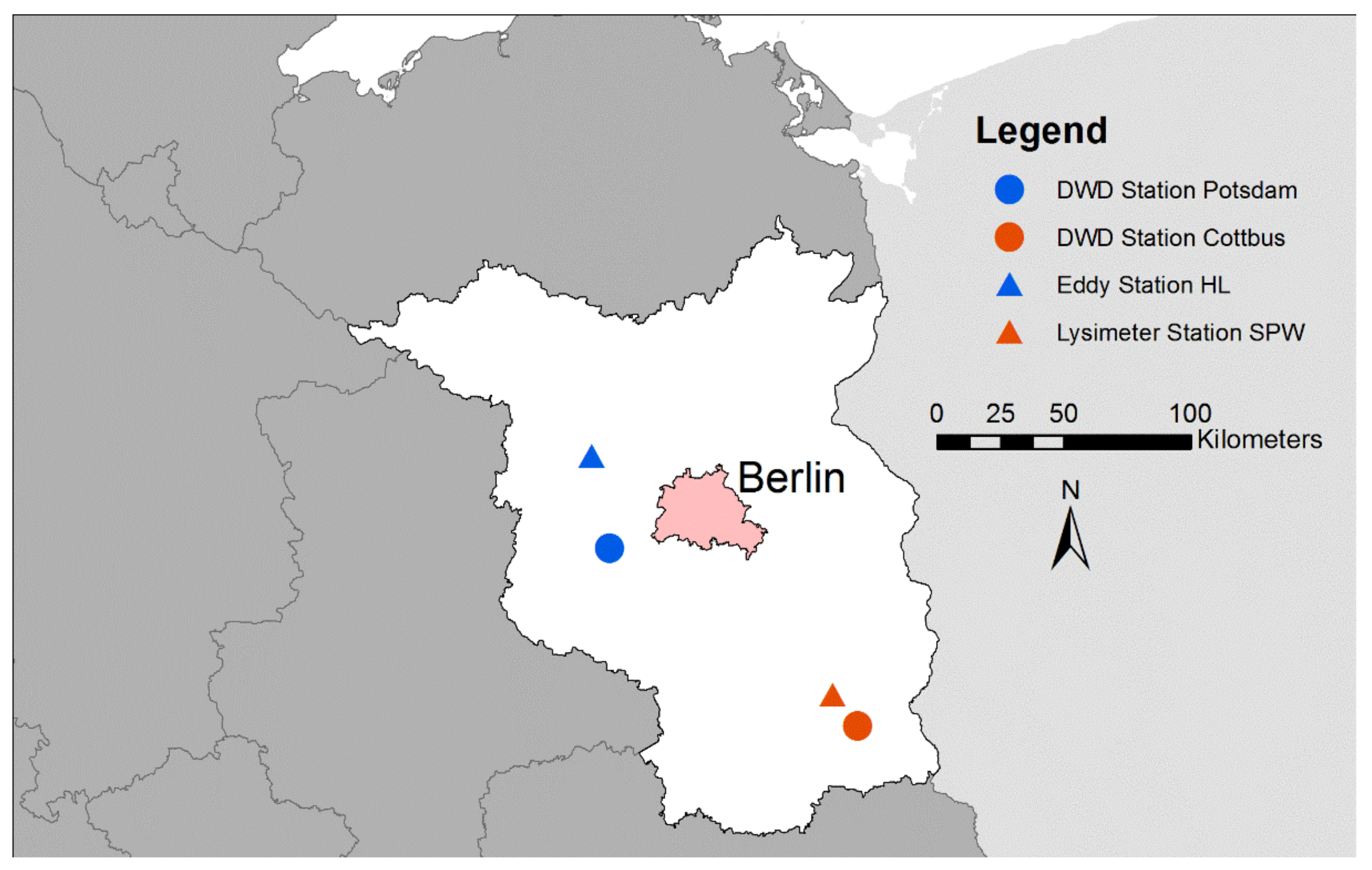
The study sites are located west of Berlin in Havelländisches Luch (HL, 52°41′ N, 12°44′ E, 28.5 m above sea level) and southeast of Berlin in the Spreewald wetland (SPW, 51°52′ N, 14°02′ E, 50.5 m above sea level) (Figure 1). Both sites are drained fens with shallow water tables used as wet grassland. They are about 130 km apart. The climatic conditions are, therefore, comparable, but there can also be major differences, especially in the case of locally limited heavy precipitation. The nearest DWD weather stations are in Potsdam (Po, 52°23′ N, 13°03′ E, 81 m above sea level) for HL and Cottbus (Co, 51°46′ N, 14°19′ E, 69 m above sea level) for SPW (Figure 1). Both DWD stations are located on higher ground with deep groundwater conditions outside their assigned study area.

The 30-year measurement series for the years 1961 to 1990 and 1991 to 2020 ([1] from both DWD stations are used for the long-term classification of our own measured values from the years 2015 to 2018. Daily values for the following parameters were available from the DWD stations:

• Daily average air temperature at 2 m above ground level;
• Daily average wind speed at 16 m (Co), 39.3 m, and 37.7 m (Po) above ground level;
• Daily average relative humidity at 2 m above ground level;
• Daily sum of sunshine duration at 10 m (Co) and 23 m/33 m (Po) above ground level;
• Daily sum of precipitation at 1 m above ground level;

Daily values of FAO grass reference evapotranspiration (ET₀) based on Allen et al. [2] are calculated from the measured values (Equation (1))

$$E{T}_0=\frac{0.408\times \Delta \times \left(\mathrm{Rn} - \mathrm{G}\right) + \mathsf{\gamma } \times \left(\frac{900}{\mathrm{T} + 273}\right) \times {\mathrm{v}}_2\times \left({\mathrm{e}}_{\mathrm{s}}-{ \mathrm{e}}_{\mathrm{a}}\right)}{\Delta + \mathsf{\gamma } \times \left(1+0.34\times { \mathrm{v}}_2\right)}$$

(1)

where Δ is the slope of the vapor pressure saturation curve in kPa C⁻¹, Rn is the net radiation, G is the ground heat flux both in MJ m⁻² d⁻¹, γ is the psychrometer constant in kPa °C⁻¹, T is the air temperature in °C, v₂ is the wind speed at 2 m above ground in m s⁻¹, (e_s–e_a) is the saturation deficit of the air in kPa. All parameters required in Equation (1) are calculated from the basic measured values according to the recommendations by [3].

Subsequently, the daily values of the four parameters were combined into monthly, half-yearly, and annual values. The half-yearly values for April to September are referred to as the summer half-year and the values for October to March as the winter half-year.

In addition to the air temperature, precipitation P, and ET₀, the climatic water balance (CWB) is used to assess the long-term climatic characteristics of the sites in the measurement years from 2015 to 2018.

$$CWB=P-E{T}_0$$

(2)

The measurement sites in HL and SPW are equipped with automatic weather stations for recording the air temperature, precipitation, net radiation, ground heat flux, relative humidity, and wind speed. The weather station in SPW measures at 1-min intervals. In HL, the sensors are part of an eddy covariance station that measures at 20 Hz and stores 15-min values. The measured values are aggregated to form daily average values or daily sums. ET₀ and CWB are then calculated from the daily values according to Equations (1) and (2).

The groundwater levels on the study sites are measured at several measuring points with automatic groundwater loggers. Of these, one representative measuring point in HL and one in SPW, which is located in the center of the site, is selected for evaluation. The water levels are stored at 15-min intervals and then aggregated into daily mean values. In the HL measurement series, there is a data gap of 19 days in May/June 2015.

The actual evapotranspiration (ET_a) is determined using different methods in HL and in SPW. ET_a is measured with an eddy covariance station at the HL study site and with a weighable groundwater lysimeter at SPW. Both methods are frequently used in wetlands [4]. Eddy covariance stations have been used, for example, to measure the ET_a of wet grasslands [5,6,7,8,9], sedge stands [8,10], or reeds [11,12,13]. Lysimeters used at wetland sites are often specially constructed [14,15,16,17]. These lysimeters are often not weighable and only determine the ET_a via the measured inflows and outflows. Both measurement methods (lysimeters and eddy covariance systems) have advantages and disadvantages, which are described in detail in Allen et al. [18].

The eddy covariance station at HL uses a CSAT3 ultrasonic anemometer to measure the wind components and an LI-7500 to measure the water content of the air. All radiation components are measured using a CNR1 and the ground heat flux with ground heat flux plates. The software package TK3 is used for processing the measured 20 Hz values and determining the latent and sensible heat flux [19]. The data quality is evaluated and valid datasets are selected using Foken’s evaluation system [20,21]. Based on the 30-min values for the net radiation, ground heat flux, latent heat flux, and sensible heat flux, the energy balance gap is then closed using the Bowen ratio method [22,23,24,25]. Finally, the corrected 30-min ET_a values are aggregated into daily values for the evaluation. Data gaps were not filled.

At SPW, a weighable groundwater lysimeter station is used to measure ET_a. The technical equipment at the lysimeter station and the associated weather station, data acquisition, and data evaluation are described in detail in Dietrich et al. [26]. For the evaluations in the article, the values measured by the station’s reference lysimeter are used. The water table depth in this monolith is controlled according to the measured water table depth at the observation well next to the lysimeter station. Since the soil in the lysimeter monolith and the vegetation on the lysimeter correspond to the site conditions of the surrounding wet grassland area, the measured water balance values are representative of these. The measured hourly ET_a values are summarized into daily values for the evaluation.

Daily crop coefficient values (K_c) are calculated from the ET_a and ET₀ for all days on which a daily value for ET_a and ET₀ is available. For the calculation of K_c, we used only days with daily values of ET₀ > 0 and ET_a ≥ 0.2 mm/d because the measurement uncertainties at very small ET_a and ET₀ values might lead to large errors in the calculation of K_c.

$$K_c=\frac{E{T}_a}{E{T}_0}$$

(3)

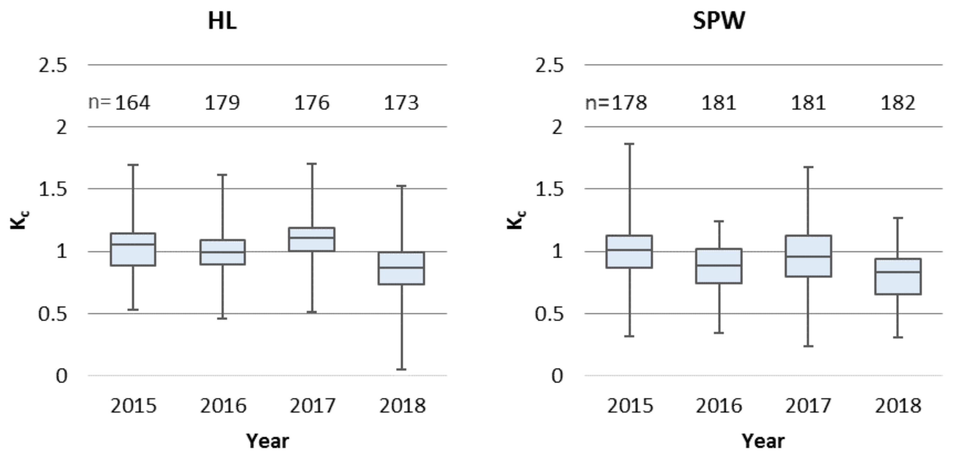
The whisker plots summarize all K_c values < 2 during the vegetation period from April to September. All comparisons of annual and half-yearly values are tested for significance using single analyses of variances (ANOVA) and T-tests. The test for normal distribution is carried out with the Kolmogorov–Smirnov test.

3. Results and Discussion

3.1. Long-Term Climatic Characteristics

The long-term meteorological parameters of the two DWD stations have comparable climatic characteristics (

Table 1. Annual and half-yearly average of the air temperature (T), sums of precipitation (P), FAO grass reference evapotranspiration (ET₀), and climatic water balance (CWB) for the 1961/1990 and 1991/2020 time series at DWD stations in Potsdam and Cottbus.

DWD Station		T	P	ET0	CWB	T	P	ET0	CWB
		In °C	In mm	In mm	In mm	In °C	In mm	In mm	In mm
	Time Series	1961–1990				1991–2020
Potsdam		January–December				January–December
	Min	7.4	377	511	−294	7.4	346	528	−438
	Average	8.7	585	600	−15	9.8	578	630	−55
	Median	8.7	599	597	−11	9.8	581	625	−63
	Max	10.1	786	691	192	11.3	798	783	189
		April–September				April–September
	Min	13.1	154	415	−393	13.9	167	445	−504
	Average	14.5	328	495	−167	15.8	326	529	−205
	Median	14.7	334	491	−149	15.7	313	523	−183
	Max	15.7	434	574	−30	18.4	521	671	15
		October–March				October–March
	Min	0.4	126	73	19	0.8	160	83	61
	Average	2.9	257	105	152	3.9	252	102	149
	Median	2.9	252	105	140	3.7	259	104	155
	Max	5.4	435	133	323	5.9	331	123	245
Cottbus		January–December				January–December
	Min	7.9	335	529	−275	7.8	353	537	−328
	Average	9.0	563	583	−21	10.1	566	629	−62
	Median	8.8	554	571	−35	10.1	558	626	−34
	Max	10.6	865	712	330	11.4	817	732	238
		April–September				April–September
	Min	13.5	104	420	−411	14.4	149	440	−429
	Average	14.8	337	477	−140	16.0	324	519	−194
	Median	14.8	344	474	−139	16.1	312	513	−168
	Max	15.9	473	549	50	18.3	498	615	15
		October–March				October–March
	Min	0.3	112	84	16	1.2	129	92	24
	Average	3.1	226	107	119	4.1	242	112	130
	Median	3.0	228	100	107	3.9	245	114	133
	Max	6.0	393	170	281	6.1	322	133	222

). The mean annual temperatures at the Cottbus station are about 0.3 K warmer than at the Potsdam station in both time series. In Potsdam, on the other hand, there is slightly more precipitation, and the ET₀ is also slightly higher compared to Cottbus. As a result, the differences in the CWB are almost balanced again.

At both stations, there is a significant increase in the average annual air temperature and the annual sum of ET₀ for the 1991/2020 time series compared to 1961/1990 (p < 0.001). Precipitation decreases slightly in Potsdam (−7 mm) and increases slightly in Cottbus (+3 mm). The changes in precipitation are not significant. The mean deficit in the CWB increases at both stations (approx. −40 mm, Table 1) due to the increase in ET₀. Only the increase in the deficit at the Cottbus station in the vegetation period is significant (p < 0.01).

The T-tests for the annual and half-yearly values show significant differences comparing the temperature series from Potsdam and Cottbus for the two time series and between the 1961/1990 and 1991/2020 time series at the two stations (p < 0.001). The ET₀ values of the 1961/1990 series of Potsdam and Cottbus also differ significantly for the annual values (p < 0.01) and the growing season (p < 0.001), but not in the winter half-year. Both half-yearly values of ET₀ for the 1991/2020 series also differ significantly (p < 0.01). There are no significant differences between the precipitation values for the two time series at the two stations. The two stations only differ weakly significantly (p < 0.05) for the 1961/1990 period.

The comparisons of the time series and the stations show that significant warming occurred at both stations from 1961/1990 to 1991/2020, but not in the average precipitation pattern. This confirms the changes in the climatic conditions of the region due to climate change [27]. The increase in ET₀ associated with the rise in temperature also leads to an increase in ET_a, especially in landscape elements with sufficient water availability (water bodies, wetlands), and thus, leads to changes in the landscape water balance [28,29].

3.2. Classification of the 2015 to 2018 Study Years in Long-Term Climate Series

Table 2. Meteorological key numbers from 2015 to 2018 in Havelländisches Luch (HL) and Spreewald (SPW) (station failures in HL: * 15 days in May/June 2015, ** 9 days in October 2016, 2 days in December 2016, in SPW: *** 2 days in August 2015, T—average air temperature, P—sum of precipitation, ET₀—sum of FAO grass reference evapotranspiration, CWB–sum of climatic water balance).

	HL				SPW
Year	T	P	ET0	CWB	T	P	ET0	CWB	Classification
	In °C	In mm	In mm	In mm	In °C	In mm	In mm	In mm
	January–December
2015	9.8	588	621 *	−33	9.6	529	666 ***	−136	average year
2016	9.4	420	693 **	−273	9.4	505	638	−132	average year
2017	9.5	783	657	126	9.5	650	649	1	wet year
2018	10.2	359	829	−470	10.1	325	787	−462	dry year
	April–September
2015	14.5	278	499 *	−222	14.6	295	554 ***	−259	average year
2016	15.4	210	585	−376	15.3	253	547	−294	average year
2017	14.6	512	525	−13	14.8	400	529	−128	wet year
2018	16.8	181	696	−516	17.0	153	667	−514	dry year
	October–March
2015	5.0	310	122	189	4.6	234	111	123	average year
2016	3.2	211	108 **	103	3.1	249	89	160	average year
2017	4.4	271	132	139	4.1	250	120	130	wet year
2018	3.5	179	132	46	3.2	173	120	53	dry year

summarizes the most important meteorological parameters of the HL and SPW study sites in the four study years. In the measurement series from HL, there are gaps on 15 days in 2015 and 11 days in 2016, and in SPW, there are gaps on 2 days in 2015. The measured values show that the four years differ significantly, not only in terms of precipitation. The extremely dry year 2018 also has the highest annual average temperature and the highest ET₀ at both locations. At the DWD stations, the 2018 annual sum is the maximum value of the 30-year series in each case, and in the study areas, the ET₀ still exceeds the maximum value of the 30-year series of the neighboring DWD station. In HL, the annual CWB deficit in 2018 is −470 mm; in SPW, it is −462 mm. The precipitation, temperature, and ET₀ in 2018 deviate from the other years, especially in the vegetation period (April to September), and lead to a deficit in CWB of −516 mm in HL and −514 mm in SPW (Table 2).

The year 2017 has the highest precipitation sum of the four measurement years at both sites, with the precipitation in HL standing out more clearly from the other years than in SPW. This applies to both the annual sums and the sum of the vegetation period. Compared to the 30-year series, however, the SPW values in particular are still well below the maximum values measured at the DWD station in Cottbus. The average temperatures and the yearly and half-yearly ET₀ values for 2017 do not differ from the values for the years 2015 and 2016.

At both sites, the measured values for the four winter half-years (October–March) are more balanced than in the vegetation period. Only the precipitation in the 2018 winter half-year is also significantly below the values for the other three years (Table 2).

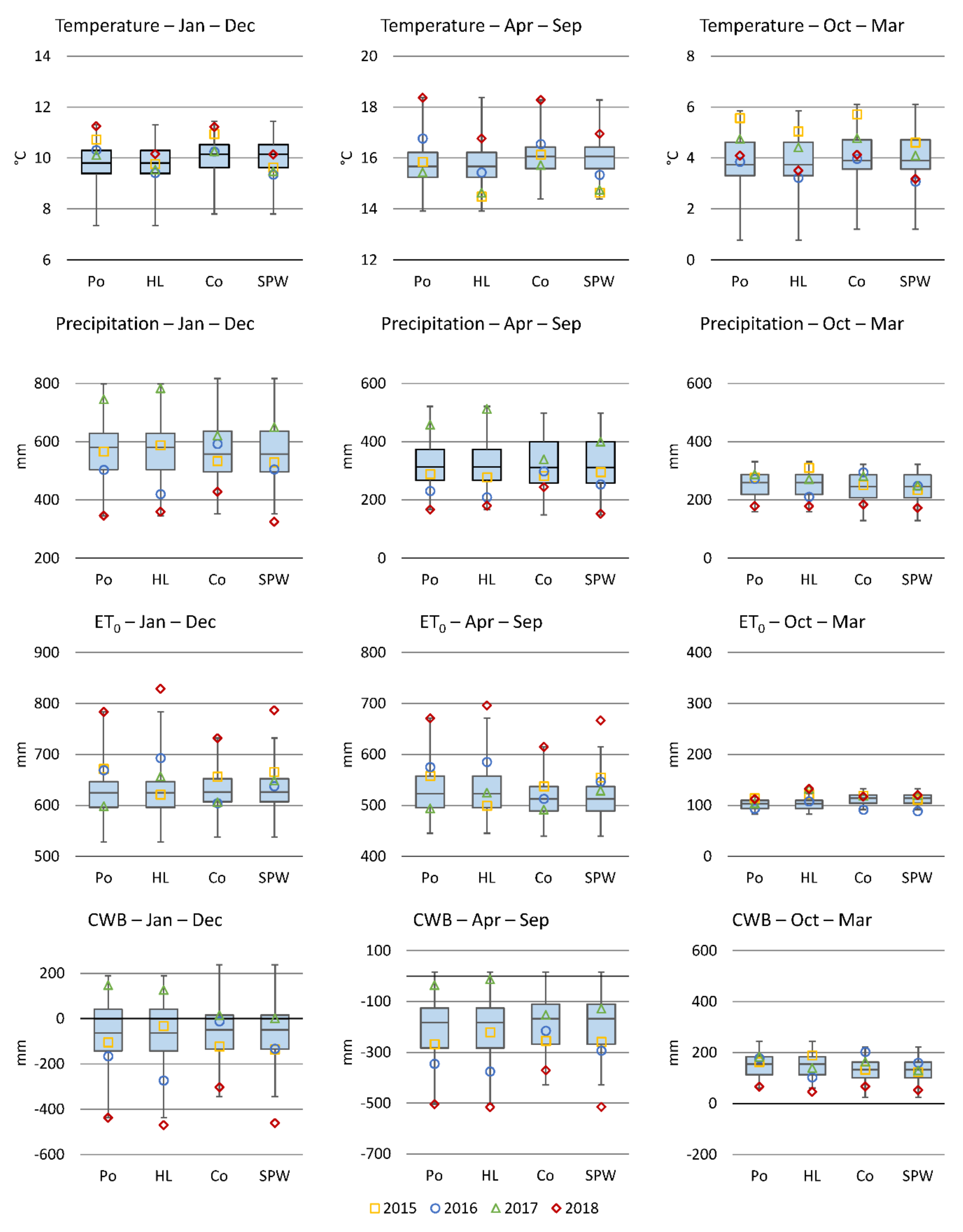
Figure 2 shows the classification of the values measured at both wet grassland sites from 2015 to 2018 in the 30-year series from 1991 to 2020 at the neighboring DWD stations. The whisker plots stand for the distribution of the values measured in the 30-year series at the two DWD stations and the dots stand for the values from the years 2015 to 2018 at the DWD stations or the study sites. The HL values are assigned to the Potsdam station and the SPW values to the Cottbus station.

The annual and half-year temperatures at the study sites fit into the 30-year long-term series. However, the values measured at the DWD stations are all higher than the temperatures measured at the study sites in the four years. While all four years are above the median values at the DWD stations, the values at the study sites tend to remain below them (Figure 2). The values for the 2015 to 2017 summer half-years are comparatively cool compared to the DWD station values; only 2018 was warmer than average even in the wet grassland areas. The overall lower temperature values are based on the well-known cooling effect that wetlands have due to their higher ET_a compared to their surroundings [11,29,30,31,32].

The ranges of the precipitation values during the four years almost reach the ranges from the 30-year series. While the values for the year with the highest precipitation at the Potsdam station are almost reached in HL, the values for 2017 at SPW are only in the range of the 3rd quartile. Peak values reached in earlier years at the Cottbus station are still far lower. In the dry year 2018, the values in HL were still significantly below the driest year of the 30-year series in Potsdam. In SPW, they correspond to the driest year of the Cottbus series. The years 2015 and 2016 are also below the median of the long-term series and tend more towards the dry years. The winter half-years in particular were all too dry.

The annual ET₀ values at the two wet grassland sites (see Table 2) are all above the long-term median values of the DWD stations (Table 1), and in 2018, the values at the study sites are also above the long-term maximum values of the DWD stations. This difference may be due to different input data used for the calculation of ET₀. The net radiation and soil heat flux used as input in Equation (1) are measured directly at the weather stations at the two grassland study sites. To calculate ET₀ at the DWD stations, the net radiation values are derived from the measured sunshine duration. The absolute ET₀ values are, therefore, only comparable to a certain degree. However, this does not restrict the comparison of the years 2015 to 2018 with each other or the comparison of the two study sites, HL and SPW. In HL, the ET₀ in 2016 is higher than in SPW despite the data gaps in October and December and deviates more clearly from the average conditions of the long-term series. The neighboring DWD stations in Potsdam and Cottbus have comparable deviations. This confirms that the stations are representative of the correspondingly assigned study areas and also confirms the regional differences between the two study regions, which are approx. 130 km apart.

The CWB values illustrate how different the meteorological conditions are in the four study years. The annual totals of CWB in HL are +126 mm in 2017 and −470 mm in 2018, and in SPW, they vary between +1 mm for 2017 and −462 mm for 2018 (Table 2). The year 2018, thus, shows extreme water deficits at both sites. According to climate model calculations, these conditions are to be expected more frequently in the coming decades [33]. The CWB in 2017 is the only year with a balance surplus at both sites and is classified as a wet year. However, the values do not reach the maximum values from the long-term series. The years 2015 and 2016 fall in between. They are classified as medium years in the further evaluations.

3.3. Effects on Groundwater Levels

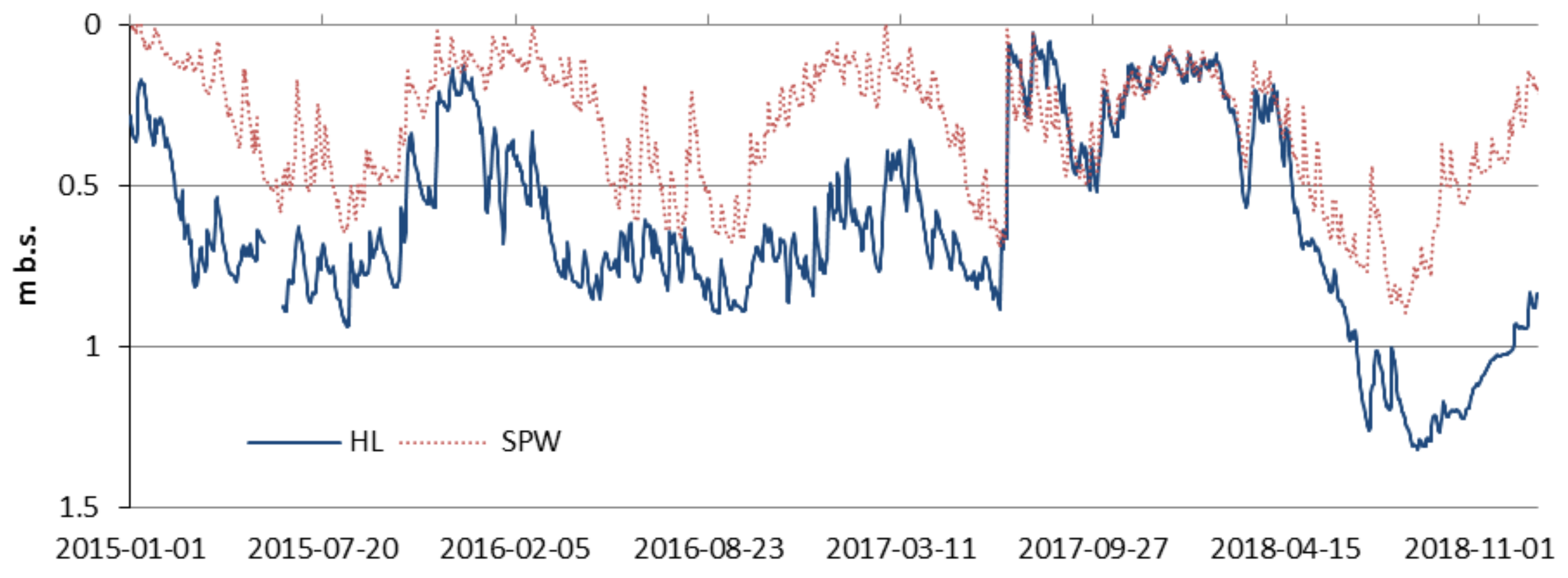
The hydrograph of the water levels in the four years under investigation mainly follows the meteorological conditions at the two sites (Figure 3, Table 2). With the development of vegetation and the resulting increase in transpiration in spring, the water levels fall continuously. In between, individual precipitation events lead to short-term rises in the water levels. The water levels in SPW are at a somewhat higher level than in HL. The reason for this is that the area is used more extensively for agriculture overall in SPW compared to HL. This is associated with higher target groundwater levels and less drainage in winter. In the two years with average meteorological conditions (2015 and 2016), the water levels drop to around 65 cm below ground level during the summer in SPW and to 90 cm below ground level in HL. In the following winters, they rise to ground level in SPW. In HL, the maximum winter levels are approx. 30 cm below ground level. The lower initial level in spring in HL continues throughout the year in years with average meteorological conditions and also always leads to a lower drop in the groundwater levels in summer compared to SPW.

In the extremely wet year 2017 and the extremely dry year 2018, there are significant differences in the water level hydrograph compared to the mean climatic conditions in previous years at both sites. In spring 2017, water levels drop until the end of June, as in previous years and, then, rise sharply with the extreme precipitation at the end of June/beginning of July. In HL, the water levels rise significantly higher than in SPW. Large parts of the study area in HL are under water for many weeks in 2017. It is not until spring 2018 that the water levels drop again to the normal level for the areas. Such high water levels are atypical for grassland used areas in Germany [34]. Overall, higher water levels can help to reduce the greenhouse gas emissions from drained peatlands [35,36,37]. The wet year 2017 is followed by an extremely dry and evaporation-intensive phase, which leads to very low groundwater levels in 2018. While the groundwater levels in SPW only drop by around 80 cm to 90 cm below ground level, they fall by 110 cm in HL during the same period, dropping to 130 cm below ground level (Figure 3). Such deep water levels are also very rare on drained wetland areas in Germany such as Bechtold, Tiemeyer, Laggner, Leppelt, Frahm, and Belting [34] showed in their overview. An increase in such deep groundwater levels would increase the degradation of peatlands and increase the greenhouse gas emissions [35].

The difference between both sites is also due to the different meteorological conditions (Figure 2). Both extreme years are more pronounced in HL than in SPW, i.e., the deficit in the dry year 2018 is larger in HL (−470 mm vs. −462 mm), and in the wet year 2017, there is a slight balance surplus in HL (+126 mm) compared to a balanced CWB in SPW (+1 mm). Another reason is the different hydrological situation in the two catchments. The study areas in HL have only a small groundwater catchment with low inflows. SPW, on the other hand, has a relatively good water supply, with the Spree river catchment lying above it and the large water reservoirs it contains [38]. This means that the extremely dry conditions in particular can be compensated for better. This confirms the model studies of Dietrich, Steidl, and Pavlik [38] for the entire Elbe river lowland.

3.4. Effects on Evapotranspiration

The different measurement methods have no discernible influence on the measured ET_a values, although the area size on which the measured values are based differs greatly depending on the measurement method. The lysimeter values (SPW) are based on an area size of one square meter, and the same area is always considered. Biomass harvesting occurs twice a year on the entire lysimeter area (mid-June, beginning of September) and, then, leads to an abrupt decrease in ET_a on the lysimeter area. In June, in a period of 10 to 14 days after the cutting date, the vegetation grows up again to such an extent that the high ET_a values from the period before the cutting are reached again. In September, the growth of the vegetation is much slower and the values before the cutting date are no longer reached in the same year. The values measured at the eddy covariance station are based on an area of origin (footprint) of several hundred to a thousand square meters, which changes constantly depending on wind direction and wind speed. This means that the site conditions of the respective footprint can also change. The wet grassland areas surrounding the eddy station are not mown uniformly on a single day; in some cases, they are also grazed. The decline in ET_a values after a cutting date is, therefore, not as clearly recognizable as with the lysimeter.

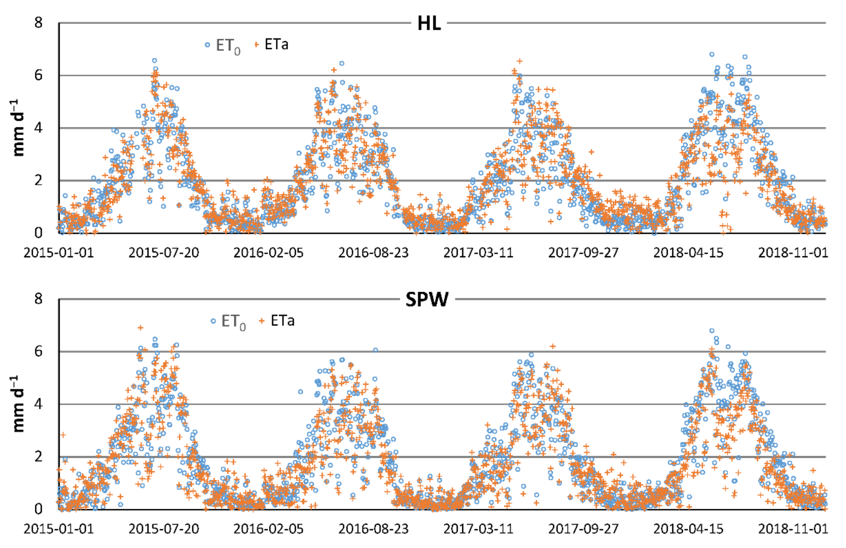
The daily ET_a values measured at both sites show the typical annual cycle that follows ET₀ (Figure 4). Both methods are, therefore, well suited for assessing how ET_a responds to the different meteorological conditions in the four study years. The daily maximum ET_a values reach 6 mm/d in all years. These are somewhat higher values than Gasca-Tucker, Acreman, Agnew, and Thompson [5] or Harding and Lloyd [6] found in southern England. However, the ET₀ values in our study regions are also higher than in southern England. Nonetheless, significantly higher ET_a values were found for other vegetation species such as reed, cattail, or silver grass [11,17,39,40,41,42]. The highest ET₀ value occurs at both sites on 2018-05-29, with 6.8 mm/d. The ET_a at the two sites does not reach the ET₀ in the summer of 2018 more often than in the summers of the previous years.

The annual sums of the ET₀ values and also the sums from April to September are significantly higher at both sites in 2018 than in the other years (

Table 3. Annual and half-year sums of FAO grass reference evapotranspiration (ET₀) and actual evapotranspiration (ET_a), along with the number of days with measured values (nET₀, nET_a) in the study years 2015 to 2018 in Havelländisches Luch (HL) and Spreewald (SPW).

Region	Period	Parameter	Year
			2015	2016	2017	2018
HL	October–March	ET0 in mm	122	108	132	132
		nET0	182	172	182	182
		ETa in mm	115	131	145	135
		nETa	167	170	162	180
	April–September	ET0 in mm	497	585	525	696
		nET0	168	183	183	183
		ETa in mm	482	565	534	538
		nETa	164	183	177	176
	January–December	ET0 in mm	618	693	657	829
		nET0	350	355	365	365
		ETa in mm	597	697	680	674
		nETa	331	353	339	356
SPW	October–March	ET0 in mm	111	89	120	120
		nET0	182	181	182	182
		ETa in mm	119	94	138	106
		nETa	182	181	182	181
	April–September	ET0 in mm	554	547	529	667
		nET0	181	183	183	183
		ETa in mm	556	487	508	547
		nETa	181	183	183	183
	January–December	ET0 in mm	666	636	649	787
		nET0	363	364	365	365
		ETa in mm	675	581	646	653
		nETa	363	364	365	364

). The sum ET_a values (Table 3) fall short of the ET₀ values in the dry year 2018, as the plant stand has an insufficient water supply. This is due to the low water table depths (Figure 3). The annual sum of ET_a in the wet year 2017 differs only slightly from the sum of the dry year 2018 (+6 mm in HL, −7 mm in SPW), although there are large differences in ET₀ (−172 mm in HL, −138 mm in SPW). The shallow unsaturated soil zone dries out strongly in 2018; the roots of the plants no longer reach the capillary fringe. As a result, ET_a is reduced, which is untypical for wet grassland sites with shallow water table conditions. In the case of the HL values, the station failures in some years must be taken into account (Table 3). Some days are, thus, missing for the ET₀ (15 days in 2015, 11 days in 2016) and ET_a (34 days in 2015, 13 days in 2016, 26 days in 2017, and 9 days in 2018).

The annual sums of the measured ET_a values, between 581 mm in SPW in 2016 and 697 mm in HL in 2016, reflect the high evaporation level of wet grassland sites. With the exception of 2017 in HL, they far exceed the respective precipitation supply and underline the sites’ dependence on inflows from their catchments [43]. As a result of the further increasing ET₀, increasing ET_a on sites with shallow water tables must also be expected as long as there is still sufficient groundwater recharge in the catchments. However, since the changed climate conditions will also affect the groundwater recharge in the catchments, changes in water availability are also to be expected in the wetlands in the future.

3.5. Effects on Crop Coefficients in the Vegetation Period

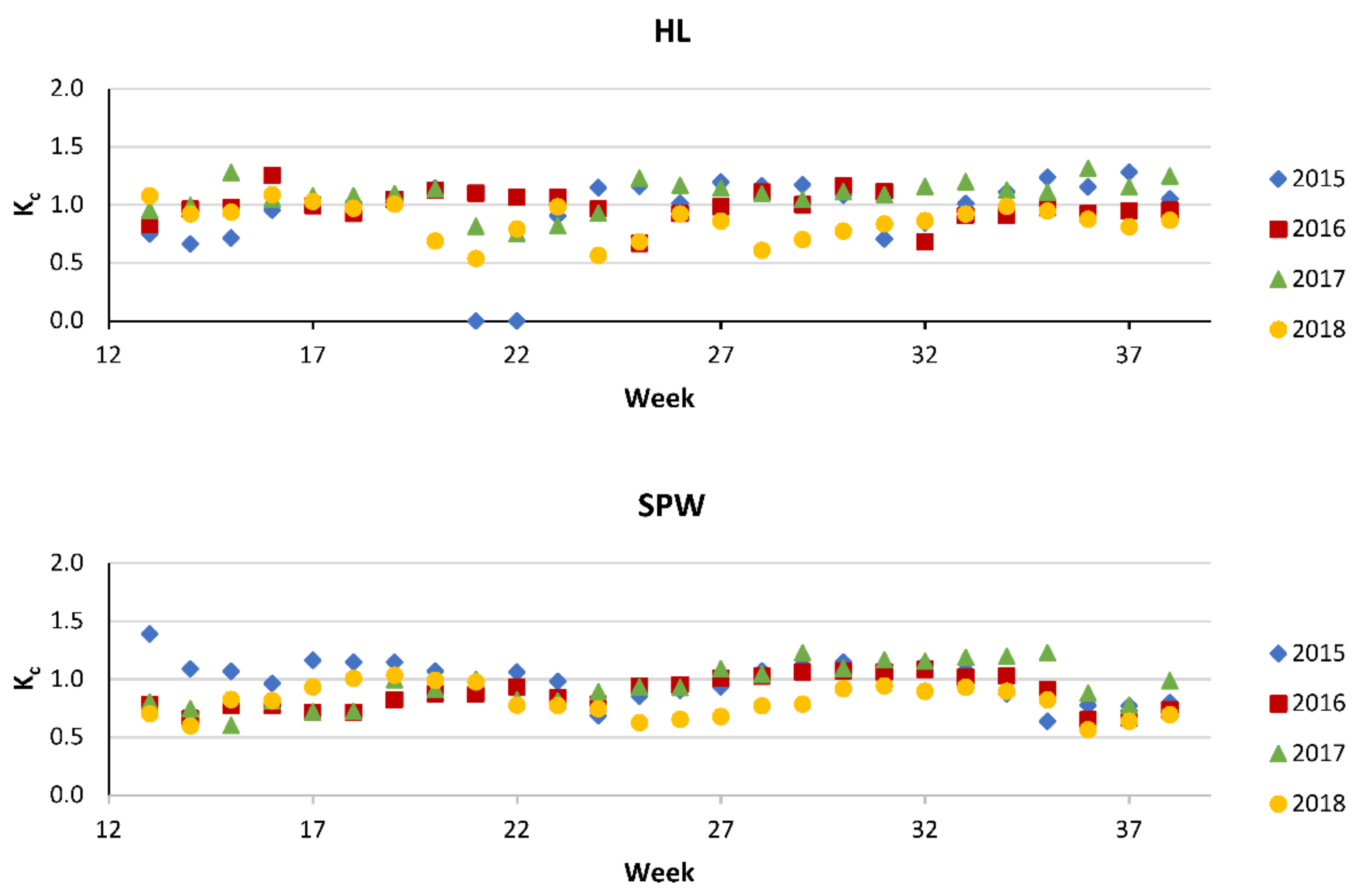
The crop coefficient K_c of a wet grassland site is influenced by various site conditions. Influencing variables include the stage of development of the vegetation, the agricultural management (cutting use with harvesting dates or grazing), and the water supply of the plants. The plant water supply is determined by the available water supply from precipitation and plant-available soil water. The latter is influenced by the soil physical properties, the water withdrawal during the previous period, and the water supply from the groundwater. The individual influencing variables cannot easily be separated due to the complex interaction of all variables on a wet grassland site with shallow water table conditions. The scattering of the weekly values for the vegetation periods at both study sites reflects these diverse impacts (Figure 5). Nevertheless, some characteristic impacts are recognizable. At the beginning of the vegetation period (week 13 to 17, early April to mid-May), the K_c values increase continuously due to vegetation development and increasing vegetation height in spring. There are no restrictions due to insufficient water supply or agricultural management effects during this period. In the period from the last ten days in May to the end of the second ten days in June (week 20 to 23), the grass stand is cut (in the HL at the end of May, in SPW only in mid-June due to nature conservation requirements). When the biomass is harvested, the K_c values decrease. They, then, increase again with the renewed growth of the grass in the following phase. The 2nd cut takes place in HL at the end of July (after week 30) and does not take place in SPW until the beginning of September (week 36). The data from SPW do not exhibit the drop in K_c values for a few days around week 30 that is found in HL. In contrast, the data from SPW clearly show the 2nd cut at the beginning of September. It can also be seen that the vegetation does not recover to its original level thereafter until the end of the month.

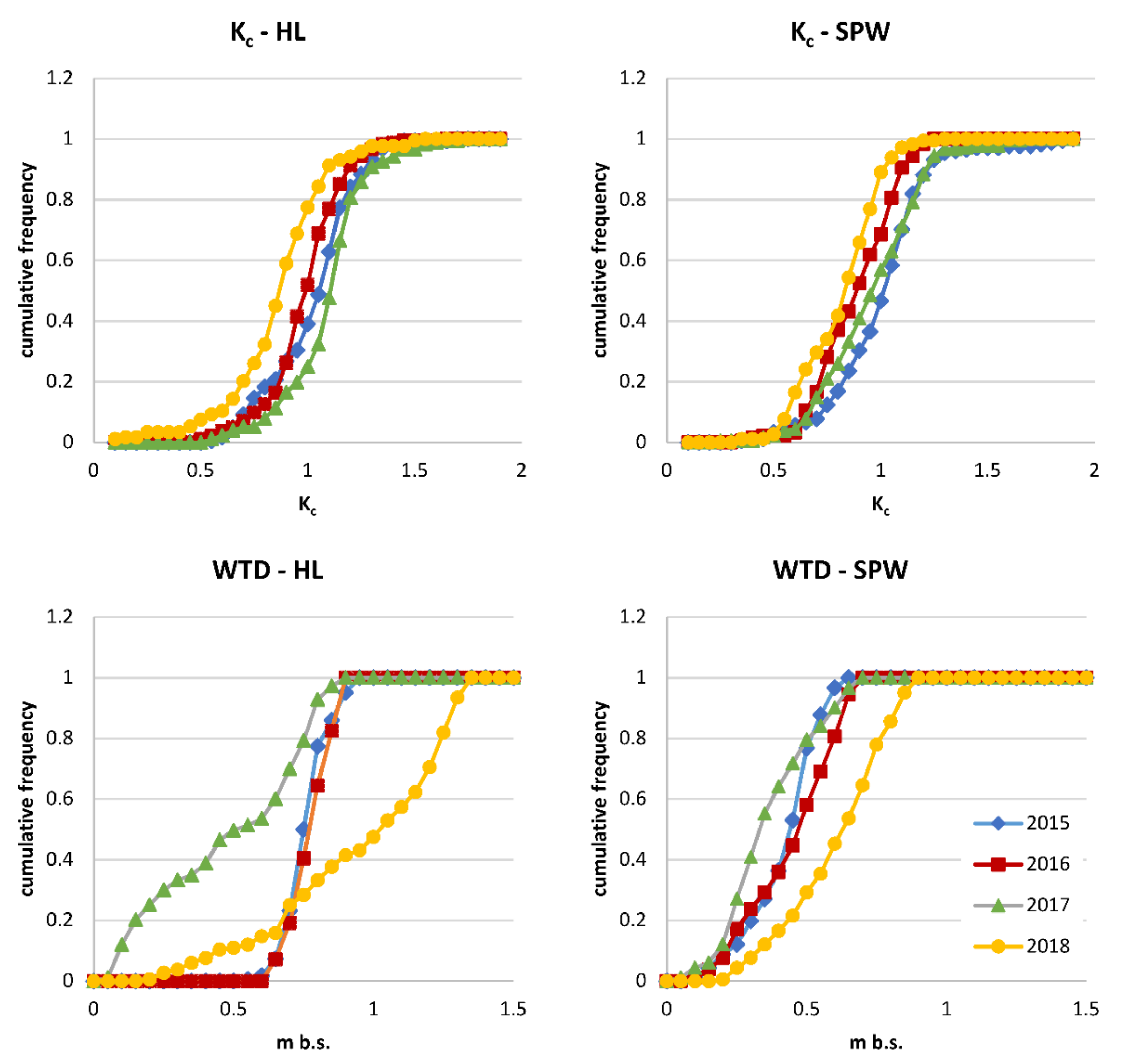
To filter out the many effects on the daily and weekly values and to highlight only the effect of the different meteorological conditions in the four vegetation periods, the entire data for the four vegetation periods were statistically compared and summarized as cumulative frequencies (Figure 6) and in whisker plots (Figure 7). It is assumed that the management impacts are repeated in all years. Minor temporal shifts in the measures have no effect on the summarized evaluation of the data. The soil-specific influencing variables change neither temporally nor spatially, meaning that changes in water availability can be attributed to the different meteorological conditions. The differences between the statistical parameters of the K_c values during the four vegetation periods can, thus, also be attributed to different meteorological conditions.

The cumulative frequencies of the K_c values and the corresponding water table depths in the vegetation periods of the four years underline the differences between the dry and wet years and their effects on the water balance (Figure 6). They show that the range between dry and wet conditions is larger in HL compared to SPW and that the K_c values are higher in HL, although the water table is almost always lower in HL.

The average K_c values in HL are highest in the wet year 2017 (HL: 1.09, SPW: 0.95) and lowest in the dry year 2018 (HL: 0.85, SPW: 0.81) (Figure 7). The median value of 1.09 in HL in 2017 shows that ET_a values often exceed ET₀. In the dry year 2018, a median value of only 0.85 is reached in HL. This underlines the fact that the crop stands received an intermittently insufficient water supply. In SPW, precipitation in 2017 was not quite as high as in HL, the median value reaching only 0.95 that year, and only 0.81 in the dry year. The overall lower values in SPW are also due to the overall less productive grass stands of the more extensively used area in SPW compared to HL. Anda, Soos, da Silva, and Kozma-Bognar [40] and Liu, Sun, McNulty, Noormets, and Fang [7] also determined K_c values around 1.0 for wet grasslands. Liu, Sun, McNulty, Noormets, and Fang [7] found that the K_c value depended on the leaf area index (LAI) and precipitation. The influence of the LAI is reflected in our results by agricultural management interventions (mowing, grazing) and also the differences between the two sites, HL and SPW. K_c values on days with precipitation events tend to lead to relatively large K_c values, as the ET₀ often approaches zero on those days, and dividing by the relatively small ET₀ value, then, leads to a large K_c value. With very small ET₀ values, measurement inaccuracies have a large influence on the calculated K_c value. The comparison of the measured K_c values for grassland with other typical vegetation types of wetland sites (reed, cattail), as they are also frequently found on renaturalized areas in the study regions, shows that these stands can achieve significantly higher ET_a values. For reeds, K_c values between 0.73 and 1.51 were found in Hungary [39,40], values between 0.4 and 1.9 in Italy [17], and values between 0.3 and 1.4 in China [12]. K_c values of up to 3.15 for reed in the UK [44] or up to 3.68 for Typha latifolia in constructed wetlands in Brazil [42], on the other hand, appear very high and are more likely to be due to other influences, such as a particularly exposed location for advective influences or the small size of the constructed wetlands.

The K_c values from the vegetation periods are all normally distributed. Their variances are between 0.03 and 0.06. All K_c values from the four vegetation periods differ significantly from each other at both sites. The T-tests from the 2015/2016 comparisons in HL and 2015/2017 in SPW reveal values of p < 0.05. All other p-values are less than 0.01. In the year-by-year comparison, the two sites differ highly significantly in 2016 and 2017 (p < 0.001) and significantly in 2018 (p < 0.05). The K_c values at the two sites do not differ significantly in 2015.

The smaller range of values between the 1st and 3rd quartile in HL is also due to the measurement method. The footprint of the eddy covariance measurement covers a much larger area than the base area of the lysimeter. This means that a greater heterogeneity in the plant stand is recorded and averaged, which has a balancing effect on the measured values compared to the small lysimeter area. Harvest dates, which always affect 100% of the measured area on the lysimeters, lead to an abrupt change in the K_c values on the lysimeters from large to very small values (0.96 → 0.67, average values 5 days before and after the cutting date). With the larger area of the eddy covariance measurement, the entire area is not harvested on one day, and spatially changing footprints further mix the harvesting effect. This highlights the typical problem of small area point measurements when transferred to the larger area [18].

4. Conclusions

Meteorological conditions such as those that prevailed in 2017 and 2018 may, according to current knowledge, occur more frequently in the future due to climate warming. Thus, the measured water balance variables are, therefore, a very suitable means of assessing how extreme meteorological conditions will affect the future water balance of wet grassland sites with shallow water table conditions.

The measured water balance variables show how differently the meteorological conditions in dry or wet years affect the groundwater hydrograph, the ET_a, and the K_c coefficient of two shallow water table sites. The values measured at both sites reflect the typical annual variation in ET_a, which is determined by meteorological conditions, vegetation development, and water availability in the soil. However, the short-term impacts of agricultural management measures are also recorded well using both measurement methods. They are, therefore, suitable for analyzing how ET_a reacts to the different conditions during the study period.

The annual sums of the measured ET_a values reflect the high evaporation level of wet grassland sites. As they far exceed the respective precipitation supply, with the exception of 2017 in HL, they demonstrate that the sites depend on the inflows from their catchment areas. How long these can meet the sites’ high water demand is a question that remains to be answered. The lower ET_a values in 2018 compared to ET₀, which are also expressed by K_c values smaller than 1, are because the plant stand’s water supply was temporarily insufficient. This is currently a relatively rare condition at shallow water table sites. If these conditions occur too frequently, the groundwater levels drop over long periods to values untypical of wetlands (<1 m below ground level), and the wetland character is lost. In particular, sites without sufficient inflows from the catchment area may, therefore, be endangered in their future existence. In order to maintain the wetland character of these areas in the long term, water retention in the wetland areas must be improved, for example, or the water consumption of other uses in the catchment area should be reduced.