
Design and Simulation of Stormwater Control Measures Using Automated Modeling
by
 , , and
Matej Radinja
1 ,
,
Mateja Škerjanec
1,
Sašo Džeroski
2,
Ljupčo Todorovski
3 and
Nataša Atanasova
1,* 1
Faculty of Civil and Geodetic Engineering, University of Ljubljana, 1000 Ljubljana, Slovenia
2
Department of Knowledge Technologies, Jožef Stefan Institute, 1000 Ljubljana, Slovenia
3
Faculty of Public Administration, University of Ljubljana, 1000 Ljubljana, Slovenia
*
Author to whom correspondence should be addressed.
Water 2021, 13(16), 2268; https://doi.org/10.3390/w13162268
Submission received: 14 July 2021
/
Revised: 4 August 2021
/
Accepted: 17 August 2021
/
Published: 19 August 2021
(This article belongs to the Special Issue Advances of Low Impact Development Practices in Urban Watershed)
Abstract
:Stormwater control measures (SCMs) are decentralized technical elements, which can prevent the negative effects of uncontrolled stormwater flow while providing co-benefits. Optimal SCMs have to be selected and designed to achieve the desired hydrological response of an urban catchment. In this study, automated modeling and domain-specific knowledge in the fields of modeling rainfall-runoff (RR) and SCMs are applied to automate the process of optimal SCM design. A new knowledge library for modeling RR and SCMs, compliant with the equation discovery tool ProBMoT (Process-Based Modeling Tool), was developed. The proposed approach was used to (a) find the optimal RR model that best fits the available pipe flow measurements, and (b) to find the optimal SCMs design that best fits the target catchment outflow. The approach was applied to an urban catchment in the city of Ljubljana, Slovenia. First, nine RR models were created that generally had »very good« performance according to the Nash–Sutcliffe efficiency criteria. Second, six SCM scenarios (i.e., detention pond, storage tank, bio-retention cell, infiltration trench, rain garden, and green roof) were automatically designed and simulated, enabling the assessment of their ability to achieve the target outflow. The proposed approach enables the effective automation of two complex calibration tasks in the field of urban drainage.
1. Introduction
Stormwater control measures (SCMs), also known as Sustainable urban drainage systems (SUDS), Low impact development (LID), Best management practices (BMP), Water sensitive urban design (WSUD), and Nature-based solutions (NBS) [1,2], are technical elements that are designed to prevent and mitigate negative effects of uncontrolled stormwater flow (e.g., urban floods or excessive combined sewer overflows) [3,4]. Common to all of them is a decentralized (or on-site) approach to rainwater management by using processes typical for the natural water cycle (e.g., infiltration, retention …) while providing ecosystem services and additional benefits for the city. Many studies have investigated the influence of individual SCMs on the quantity and quality of stormwater in urban sub-catchments, i.e., on a micro-scale [5,6,7,8]. Moreover, models are being used to design SCMs and predict SCM performance for different design and weather scenarios [9,10,11]. To investigate the impact of SCMs at meso-scale and macro-scale these models need to be integrated into or coupled with catchments rainfall-runoff (RR) models. Models incorporate the previously acquired knowledge on water-related physical phenomena (e.g., water percolation [12,13], surface runoff [14] …) in a form of mathematical formulations.
In this context, the open-source Stormwater Management Model (SWMM) [15] is one of the most widely used models [16,17,18,19] enabling RR and hydraulic modeling of urban drainage. It also contains several SCM elements that can be integrated within the model, after being designed by the user separately. SWMM does not enable any automation that would speed up the calibration process of the RR model. Thus, search techniques (e.g., genetic algorithms, neural networks, regression trees …) [20,21] and parameter optimization tools (e.g., PEST, OSTRICH) [22,23,24] are used to automate RR model calibration.
SCMs with predetermined design can be integrated into the RR model to simulate and evaluate their efficiency and performance through hydrological parameters (e.g., peak flow reduction, total volume …) [4,16,19]. However, SCM benefits can also be evaluated from the non-hydrological perspective (e.g., economic, social, environmental) [23]. In the above approach, the performance of SCMs is merely observed, and their optimal design for reaching a target function (e.g., allowed surface runoff or determined hydrograph), can only be achieved through an iterative expert-driven process. Therefore, approaches that encompass auto-calibration of the RR model and objective-driven automated SCM design are more favorable. Zhu et al. [25] investigated this approach by coupling SWMM and PEST [26] to auto-calibrate the parameters of the RR model and two SCMs (i.e., bio-retention cell and permeable pavement). In their study, four target hydrographs were generated, by four reductions of the original impervious cover of each sub-catchment and by simulating a 5-year, 2-h duration design rainfall. The authors reported favorable results; however, the SWMM model has some limitations (e.g., a limited number of parameters representing SCMs).
Furthermore, SWMM, similar to other mechanistic models, uses one mathematical model (predetermined by the modeler) at a time to describe hydrological processes within the urban catchment. In case there are alternative mathematical models for describing the same type of process (e.g., hydrological), their suitability needs to be investigated separately. This limits the possibilities for discovering new models that could potentially better describe the observed natural phenomena (i.e., RR). To overcome the above-mentioned drawbacks, automated modeling (AM) based on equation discovery can be used to (a) find the most suitable RR model combining the choices among multiple alternatives for describing each hydrologic process modeled, (b) to calibrate the RR model parameters against measured data, and c) to design SCMs based on a target function.
Equation discovery is an area of machine learning that develops methods for automated discovery of mathematical models, expressed in the form of equations, from collections of measured data [27]. Process-based modeling, employed in this paper, is a specific approach to equation discovery that allows for integrating domain knowledge in the process of equation discovery. The knowledge is encoded as a library that represents a collection of components for modeling systems in the domain of interest. Automated modeling by using knowledge libraries of model components has been already successfully applied for modeling aquatic ecosystems [28], watersheds [29], dynamic biological systems [30], and water-tank dynamics [31]. To the best of our knowledge, no such attempts have yet been made in the field of urban RR modeling and SCM design.
This paper provides integration of automated equation (model) discovery and domain-specific knowledge in the fields of rainfall-runoff (RR) and stormwater control measures (SCMs) modeling. More specifically, the goals of this paper are:
- To develop a library of components for modeling RR and SCMs, compliant with the equation discovery tool ProBMoT (Process-Based Modeling Tool) [32];
- To apply the proposed automated model discovery approach to find the optimal RR model for an urban sub-catchment in the city of Ljubljana, Slovenia, which best fits the available pipe flow measurements;
- To find an optimal design of SCMs that would best fit the target catchment outflow.
2. Data and Methods
2.1. Case Study Area
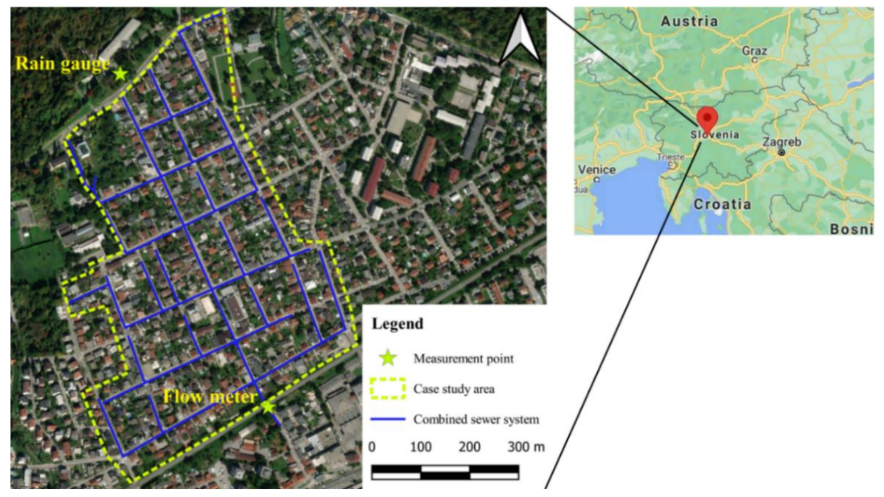
The case study area is located in the western part of the city of Ljubljana, Slovenia, and covers about 30 ha. The predominant land use in this area is family houses with gardens (Figure 1). The area has a temperate continental climate, with a mean long-term (1986–2016) annual rainfall of about 1380 mm [33]. The largest part of the area is served by a mixed sewer system with a length of approx. 5.4 km.
2.2. Data
Precipitation data were provided by the Slovenian Forestry Institute, for a rain gauge station located on the north side of the case study area (location: 46°03′06.82″ N, 14°28′47.58″ E, 306 m above mean sea level (MAMSL) [34]. The measurements were performed with a Davis® (0.2 mm) Rain Gauge Smart Sensor [35]. Data on extreme rainfalls were obtained from the IDF curves for the Ljubljana–Bežigrad weather station [36]. These served for the simulation of design rain events with a duration of 1 h, and return periods of 5, 10, 25, and 50 years, with total precipitation depth of 38 mm, 44 mm, 53 mm, and 59 mm, respectively.
The local public utility company (JP VODOVOD KANALIZACIJA SNAGA d.o.o.) provided the information on the combined sewer network and the flow measurement data. The flow measurements were performed between 1 March 2019 and 30 September 2020 in a pipe (of the combined sewer system) collecting all contributing water from the case study area (location: 46°02′44.56″ N, 14°29′01.82″ E, 295 MAMSL) (Figure 1). The flow rate was calculated based on the combination of non-contact radar velocity measurements and ultrasonic water level measurements [37]. As the focus was only on rainfall-runoff (RR) (i.e., stormwater) modeling and the measurements were conducted in a combined sewer system, the dry weather flow, which is independent of the RR and cannot be explained with the RR model, was deduced from the total measured flow. For the preparation of precipitation and flow data, a 5-min time step was used.
Within the entire flow measurement period, rainfall data were collected corresponding to the measured flow. To test the usefulness of the proposed approach for single events and continuous simulations, as defined by the EPA SWMM [15], two types of rainfall periods were selected: shorter (approximately 1 day) and longer (approximately 6 days). Four rainfall periods were selected for model calibration (C1–C4) and another four for model validation (V1–V4) (Table 1). Hence, two short (C1 and C2) and two long (C3 and C4) rainfall periods were selected for model calibration. The longer calibration periods include multiple rainfall events of different intensities and durations so that the ProBMoT tool could learn from the different surface runoff responses of the catchment. The validation periods were selected based on the following criteria: (a) duration, with shorter (V1 and V2) and longer (V3 and V4) periods; (b) seasonal distribution; (c) similarity in peak flows; (d) stability of measured flows; and (e) antecedent weather conditions [38,39].
2.3. Rainfall-Runoff Model
The rainfall-runoff (RR) model is based on the principles and equations used by the EPA Storm Water Management Model (SWMM) [15]. Variables and constants included in Equations (1)–(8) are described in Table 2 and Table 3. The catchment is represented as a nonlinear reservoir, governed by surface storage mass balance, i.e., conservation of mass:
Evaporation was not included in the model, due to its limited influence on the water mass balance within the short rainfall events used for SCM design. The runoff flow rate per unit of the surface area is based on Manning’s equation [15]:
Afterward, the total runoff flow from the catchment (L/s) is calculated by multiplying the catchment surface area (m2) and q (m/s).
There are several well-known alternative methods for modeling the infiltration process. Three alternatives were considered in this study: the Soil Conservation Service Curve Number (SCS CN) method, the Variable UK runoff equation, and the UK Water Industry Research runoff equation. Thus, the complete RR model can have different structures, depending on the infiltration method selected. In addition, different infiltration methods can be applied in different sub-catchments, resulting in many plausible model structures for a given catchment.
2.3.1. SCS CN Method
This method assumes that the total infiltration capacity of a soil is related to the soil’s tabulated Curve Number (CN). The CN value is determined by the hydrologic soil group, land use, and hydrologic condition. CN values range from 30 to 98. The latter value is assigned to paved roadways, roofs, and other impervious surfaces. At higher CN values (i.e., closer to 98), precipitation is mainly translated into surface runoff. On the other hand, at lower CN values (i.e., closer to 30), rainfall is mainly infiltrated and is thus not translated into a runoff [14]. A modified version of the SCS CN equation was used, as described in the SWMM Reference Manual-Hydrology [15]. In the modified version, the initial abstraction () is not included, as it is already included in the depression storage (; see Equation (2). The following three equations (Equations (3)–(5) are used to calculate the infiltration rate:
2.3.2. Variable UK Runoff Equation
The Variable UK runoff equation (VARUK) has three components: runoff from impervious areas, runoff from pervious areas, and initial losses [40]. It is based on data from 11 UK catchments and 112 rain events. The VARUK equation is as follows [41]:
Rainfall can be converted into infiltration by using the following equation:
2.3.3. UK Water Industry Research Runoff Equation
The UK Water Industry Research runoff equation (UKWIR) [42] was developed to overcome some of the limitations of VARUK, which are described in detail in the report Development of the UKWIR Runoff Model (2014). As VARUK, it has a fixed runoff component for paved surfaces (. It was upgraded with a variable runoff component for paved surfaces. Additionally, a component for pervious surfaces was added, which enables differentiation between winter and summer runoff (i.e., negative antecedent precipitation index (NAPI)). The UKWIR equation is then as follows:
2.4. Stormwater Control Measures
In this study, SCMs are based on the principles and equations used by SWMM for modeling low impact development (LID) controls [15]. These are bio-retention cell (BRC), rain garden (RG), green roof (GR), and infiltration trench (IF). Based on the principles and equations typical for these measures, two additional SCMs were defined, namely the detention pond (DP) and the storage tank (ST). The processes that characterize individual SCMs are described in equations 9–30. Variables and constants that are included in these equations are described in Table 4 and Table 5.
To make the computation of SCMs hydrologic performance less complex, the following simplifications are assumed by SWMM [15]: (1) the cross-sectional area of the unit remains constant throughout its depth; (2) flow through the unit is 1D in the vertical direction; (3) inflow to the unit is distributed uniformly over the top surface; (4) moisture content is uniformly distributed throughout the soil layer; (5) matric forces within the storage layer are negligible so that it acts as a simple reservoir that stores water from the bottom up.
2.4.1. Bio-Retention Cell
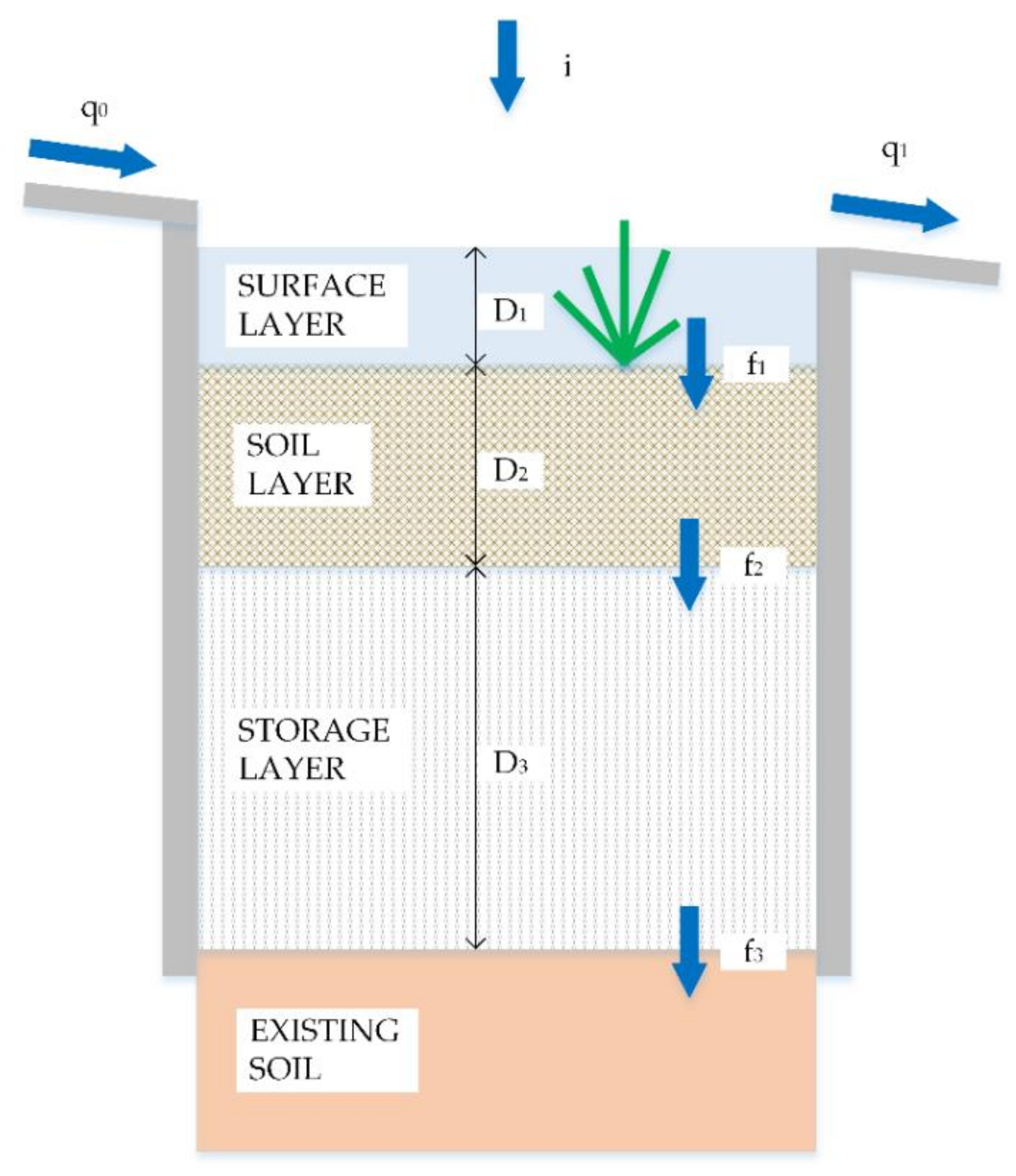
Bio-retention cells (BRCs) are depressions that contain vegetation grown in an engineered soil mixture placed above a gravel storage bed. They provide storage, infiltration, and evapotranspiration of both direct rainfall and runoff captured from surrounding areas. As such, they can be used as a generic SCM model, which can be then customized to describe the behavior of other SCM types. Due to the short length of the design rain events (i.e., 1 h); evapotranspiration was not included in the model, as it would not have a significant influence on the results. A conceptual model of a typical BRC can be represented with three overlaying horizontal layers (Figure 2). The inflow to the surface layer includes both direct precipitation (i) and captured runoff from contributing areas (). On the other hand, the outflow can occur through infiltration into the soil layer below () or by the overflow of ponded surface water (). The latter may occur if the level of ponded surface water exceeds the freeboard height of the surface layer (). The soil layer receives infiltration () from the surface layer and loses water through percolation () into the storage layer below. The storage layer receives percolation () from the soil layer above and loses water by exfiltration () into the underlying natural soil. Materials with high porosity (e.g., gravel) are used to provide water storage capacity.
Variables and constants included in the SCM equations are described in Table 4 and Table 5. Along with their original (EPA-SWMM) [15] names, the newly defined names used in ProBMoT are provided. Furthermore, Table 5 provides the minimum and maximum values of the constants.
The current amount of water within every layer can be calculated by solving mass balance equations that take into account all the inflows and outflows (Equation (9)–(11)). The infiltration rate () (Equation (12)) is based on the Green-Ampt equation, whereas for the percolation rate () (Equation (13)), Darcy’s law is used [15]. The overflow rate () (Equation (14)) is simply calculated as any ponded water that exceeds the maximum freeboard (or depression storage) height within each time step.
Water fluxes between layers are limited by the current conditions in the connected layers. Two types of conditions need to be fulfilled for infiltration to occur: (1) a sufficient amount of water is needed in the upper layer (Equations (16) and (18)), (2) a sufficient amount of empty pore space is needed in the lower layer (Equations (15) and (17)).
2.4.2. Rain Garden
SWMM defines a rain garden (RG) as a bio-retention cell without a storage layer [15]. Its governing equations are, therefore, Equations (9) and (10). The nominal soil percolation rate (Equation (13)) is limited to the smaller of the following two values: the amount of drainable water available in the soil layer (Equation (16)) and the saturated hydraulic conductivity of the native soil ().
2.4.3. Green Roof
SWMM’s green roof (GR) is also similar to a bio-retention cell, except it uses a drainage mat instead of gravel aggregate in its storage layer and has an impermeable bottom (). Therefore, the bottom exfiltration () is replaced by the drainage mat flow rate () (Equation (23)). Furthermore, there is no term for captured runoff from impervious areas () (Equation (19)). Both the runoff rate from the soil layer surface (Equation (22)) and the drainage mat flow rate () (Equation (23)) are computed by using the Manning equation for uniform overland flow.
2.4.4. Infiltration Trench
SWMM’s infiltration trench (IT) is also similar to a bio-retention cell, except that it has only a surface and a storage layer, where assumes that any ponded surface water () drains into the storage layer over the time step. Furthermore, the surface void fraction) does not appear in the surface layer equations (Equation (24)) as a gravel-filled trench would have no vegetation growing above it.
Both the infiltration and exfiltration rate are limited by the amount of water currently in the storage layer (Equations (27) and (28)):
2.4.5. Detention Pond and Storage Tank
Based on the principles and equations presented with the previously defined elements, two additional elements were defined, namely a detention pond (DP) (Equation (29)) and a storage tank (ST) (Equation (30)). They both include only a surface layer, which is deeper than with the previously defined elements. The inflow for DP includes direct rainfall and runoff from contributing areas, whereas ST receives only runoff from contributing impervious areas. For both elements, the outflow (i.e., overflow) is calculated by using q1 (Equation (14)).
2.5. Equation Discovery and Process-Based Modeling
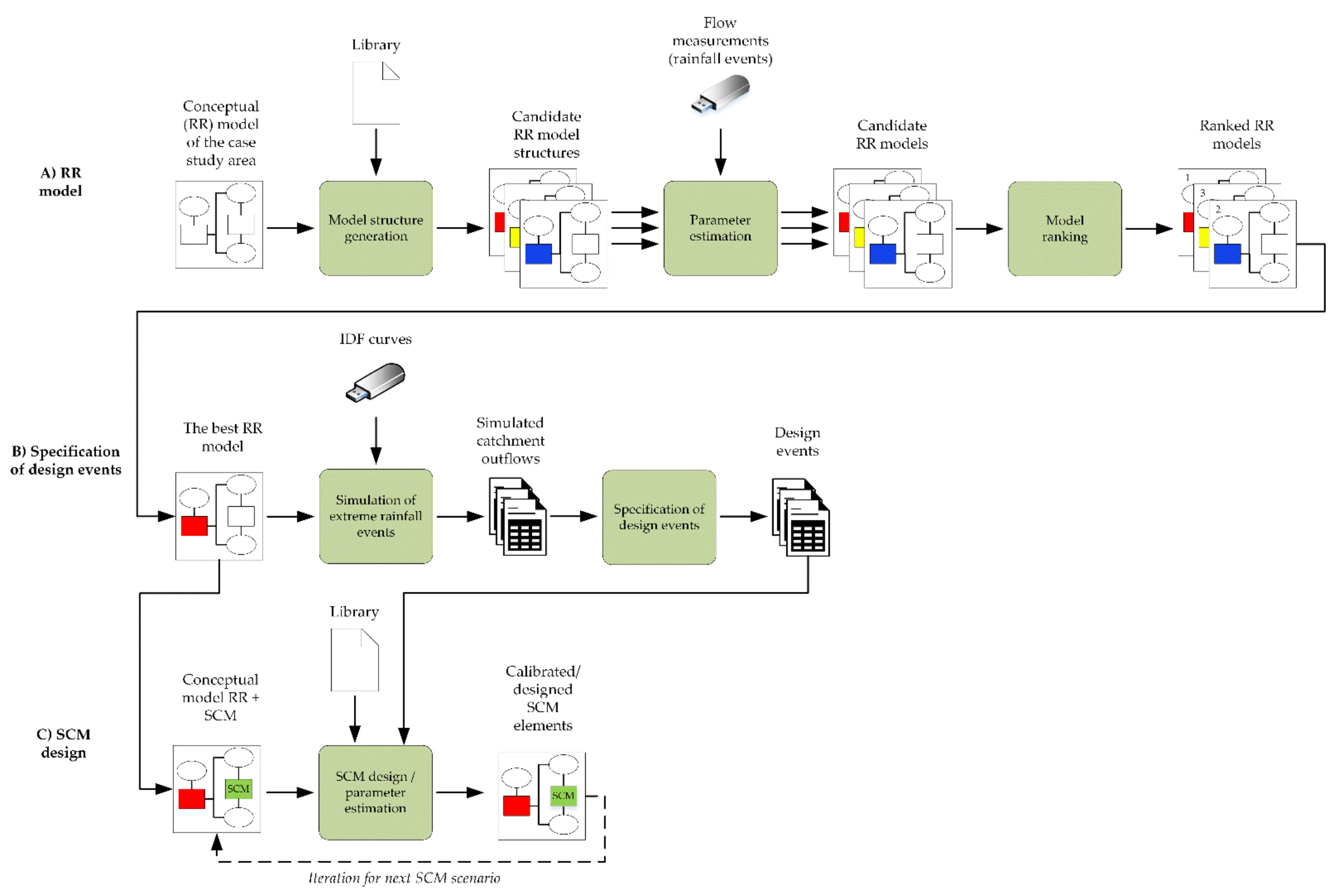
The proposed automated modeling approach is based on the Process-Based Modeling Tool (ProBMoT), developed by Čerepnalkoski et al. [43]. ProBMoT allows for the integration of domain knowledge, formalized as template components for the construction of process-based models, into the procedure of equation discovery from measured data. It automatically identifies both the structure and parameter values of an appropriate process-based model, given: (a) a knowledge library (i.e., a mathematical formulation of the selected domain) in the form of model components, or, more specifically, template entities and processes, (b) a conceptual model of the observed system, and (c) measurements (Figure 3). Candidate model structures are generated from the knowledge library and a user-specified conceptual model of the observed system. The candidate models are transformed into equations, calibrated against provided data, and ranked according to their errors. The latter is calculated as the root-mean-squared-error (RMSE), i.e., the discrepancy between the model simulation and measured data. To use ProBMoT within the presented case study of RR modeling and SCM design, the following steps were taken:
- (A.1)
- The RR models and SCM processes were encoded in a modeling library;
- (A.2)
- Conceptual models of the case study and SCM scenarios were elaborated;
- (A.3)
- ProBMoT was used to discover the optimal model structure and parameters among viable RR models, following the conceptual model of the case study and flow measurements;
- (B.1)
- The RR model with the best performance was used to simulate catchment outflow for rainfall events with a duration of 1 h and return periods of 5, 10, 25, and 50 years;
- (B.2)
- Three design events (i.e., data sets) that represent target catchment outflows were defined. The target outflow of precipitation (with a return period of 10, 25, or 50 years) was set to be the outflow typical for a 5-year return period;
- (C.1)
- ProBMoT was used to determine the optimal SCM parameters (i.e., SCM design), following the conceptual model for each SCM scenario and target catchment outflow (i.e., outflow reduction);
- (C.2)
- To determine the best SCM design, the conceptual models for SCMs were iteratively changed, based on the preliminary results of SCM design.
2.5.1. Library of Components for Modeling Rainfall-Runoff and Stormwater Control Measures
The library consists of entity templates, process templates, and compartment templates. Each template captures general knowledge that can be applied to different cases and can be reused when dealing with a specific task. The dynamic system to be modeled, i.e., the catchment, can be structured by using compartments. Compartments are organized in a nested, tree-like structure. Each compartment contains entities and processes and can also contain other sub-compartments (e.g., sub-catchments) [29]. In the urban hydrology domain, processes calculate the change of water fluxes (e.g., surface storage) within a time step and entities aggregate these changes over the simulated time.
The equations presented in Section 2.3 were encoded in the knowledge library (see Supplementary Material S1: Knowledge library) as template processes named general processes, as they are common to all the models. These include D (surface storage), Q (surface runoff), OF1 and OF3 (outflow), and F (infiltration), which can be modeled with three alternative methods: F_SCS, F_UKWIR, and F_VARUK. The SCMs equations presented in Section 2.4 were encoded in the knowledge library as template processes named after SCMs (e.g., detention pond processes). Names of processes and entities are derived from variable names and SCM type abbreviations (e.g., D1_DP). Uppercase letters are used for variable names related to processes (e.g., D1_DP) and lowercase letters for variable names related to entities (d1_DP). Outflow processes that sum the discharges from different sub-compartments (i.e., sub1, sub2, etc.) were introduced. Namely, the OF3 (i.e., the sum of discharges from an impervious and pervious area with no implemented SCMs (i.e., OF1)), the OF4_SCM (i.e., the sum of the overflow from SCMs (i.e., OF2_SCM)), and the OF5_SCM (i.e., the sum of OF3 and OF5_SCM). The time step in the presented equations is 1 s, so ProBMoT is calculating the infiltration rate in m/s and discharge in L/s. However, the actual time step of the input data (e.g., precipitation, measured flow) is 5 min, which is also the reporting time step.
2.5.2. Conceptual Models of the Case Study Area and Stormwater Control Measures
To apply ProBMoT to a specific catchment, a conceptual model of the observed system must be provided (see Supplementary Material S2: Conceptual model). The conceptual model consists of entity, process, and compartment instances. Each instance is created using a template from the urban hydrology modeling library. The specification of a process instance includes a list of arguments (i.e., names of the entity instances that are involved in the process) and a list of constants with their exact values (e.g., entity: Surface, constant: slope = 0.002). For unknown values of the constant parameters or the parameter that will be calibrated (e.g., SCM design), the parameters are assigned a special value »null«, along with its expected range of values (e.g., entity: SCM, constant: D1 {value: null; fit_range: <0, 1.5>}). The values and ranges of the constants that appear within the RR model (i.e., entity Surface) were adjusted based on the (im)perviousness of the sub-catchment (Table 3) following the values proposed in the literature [14,15,40,41,42]. The values and ranges of the constants that appear within SCMs (i.e., entity SCM) were defined based on the values proposed by EPA [15] (Table 5).
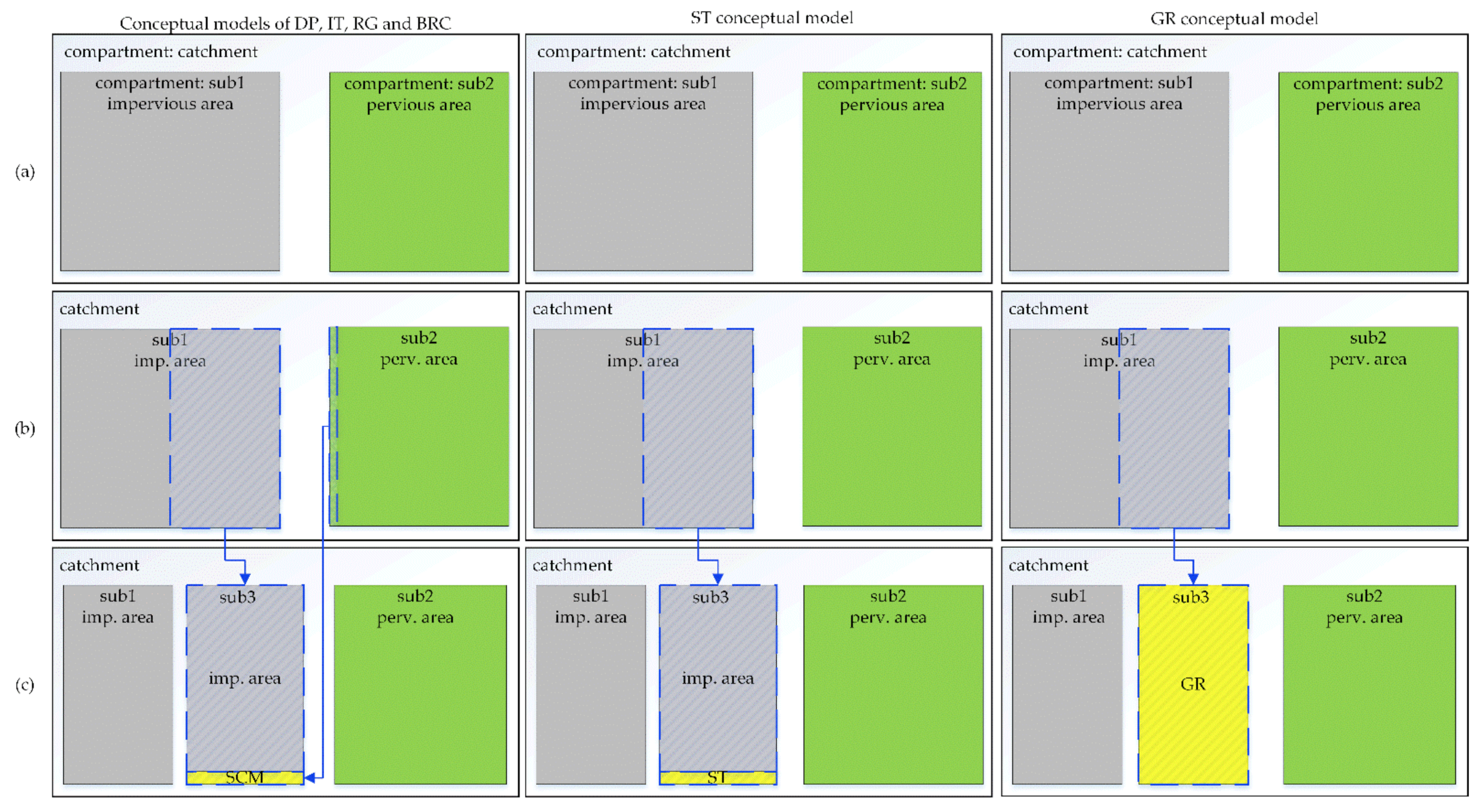
The conceptual model of the case study area (Figure 4a) was structured as a single compartment (i.e., catchment), divided into two sub-compartments (i.e., sub1 and sub2), where sub1 represents the impervious part of the catchment (60% of the total surface area) and sub2 the pervious part of the catchment (40% of the total surface area). A new sub-compartment (i.e., sub3) (Figure 4c) was introduced to account for SCMs, including SCM area and contributing areas. SCMs can be placed either within a part of an existing pervious area (DP, IT, RG, BRC) or an impervious area (ST, GR). However, in the case of GR, the measure itself also acts as a contributing area, by receiving direct rainfall. To ensure transparency, a separate conceptual model was defined for each SCM.
3. Results
3.1. Rainfall-Runoff Models
Given the conceptual model and the modeling knowledge library, ProBMoT explored nine alternative structures of RR models (M1–M9) (Appendix A Table A1). Each model chooses a different combination of modeling templates for infiltration for each of the two sub-catchments. Each of the nine models was calibrated and validated against the measured data. All models were calibrated by simultaneously using data (C1–C4) from two short time periods of measured flow, with a duration of approximately one day (C1 and C2), and two long periods of measured flow, with a duration of approximately one week (C3 and C4). The calibrated models were validated on four different rainfall periods (V1–V4) that vary in rainfall duration and intensity. The values of the Nash–Sutcliffe efficiency (NSE) coefficient [44] for the calibration and validation data sets/events are presented in Table 6. The rainfall periods are presented in consecutive order, based on the modeling phase (first calibration—C, then validation—V) and the duration of the modeled rainfall period (e.g., 1D—one day).
Based on the criteria for assessing the goodness of fit for models, proposed by Moriasi et al. [45], the models on average had »very good« performance (i.e., 0.75 < NSE ≤ 1.00) for all calibration periods. In the validation process, all models had »very good« performance for all validation periods, confirming the usefulness and efficiency of the proposed approach for calibration of model parameters. When comparing the performances of the models, differences can be noticed for individual rainfall periods. Nevertheless, they all achieved a similar average NSE value for calibration (i.e., average NSE value of 0.794) and validation periods (i.e., average NSE value of 0.859). Therefore, no general conclusion can be made about which model is better, since model performance results are greatly influenced by the characteristics of calibration and validation periods (e.g., rainfall intensity, number of (sub) rainfall events) [46]. However, the model with the highest average NSE values for the calibration and validation periods (i.e., M3) was used for further analysis.
Next, the 1-h rainfall events with return periods of 5, 10, 25, and 50 years were simulated using the calibrated model M3, resulting in a total outflow of 6429 m3, 7562 m3, 9426 m3, and 10,403 m3, respectively. Based on these results, three target catchment outflow scenarios and datasets were defined, namely the DE_Q5_P10, DE_Q5_P25, and DE_Q5_P50. These design events represent a combination of an outflow typical for 5-year precipitation (i.e., Q5) and precipitation with longer return periods (i.e., P10, P25, P50). In this way, SCMs are designed to reduce the peak and total volume of the catchment outflow.
3.2. Stormwater Control Measures
SCMs were designed to retain the difference between outflows from the catchment provided by precipitation with 10, 25, and 50 years return period (i.e., P10, P25, P50) and 5 years return period (Q5, or the target outflow). More precisely, they were designed to maximize the extent to which each SCM type can achieve the target outflow, using the proposed parameter ranges. The match between the simulated and the target outflow was evaluated using the Nash–Sutcliffe efficiency coefficient (NSE), peak flow ratio (PFR), and total volume ratio (TVR) (Appendix A Table A2, Table A3, Table A4, Table A5, Table A6 and Table A7).
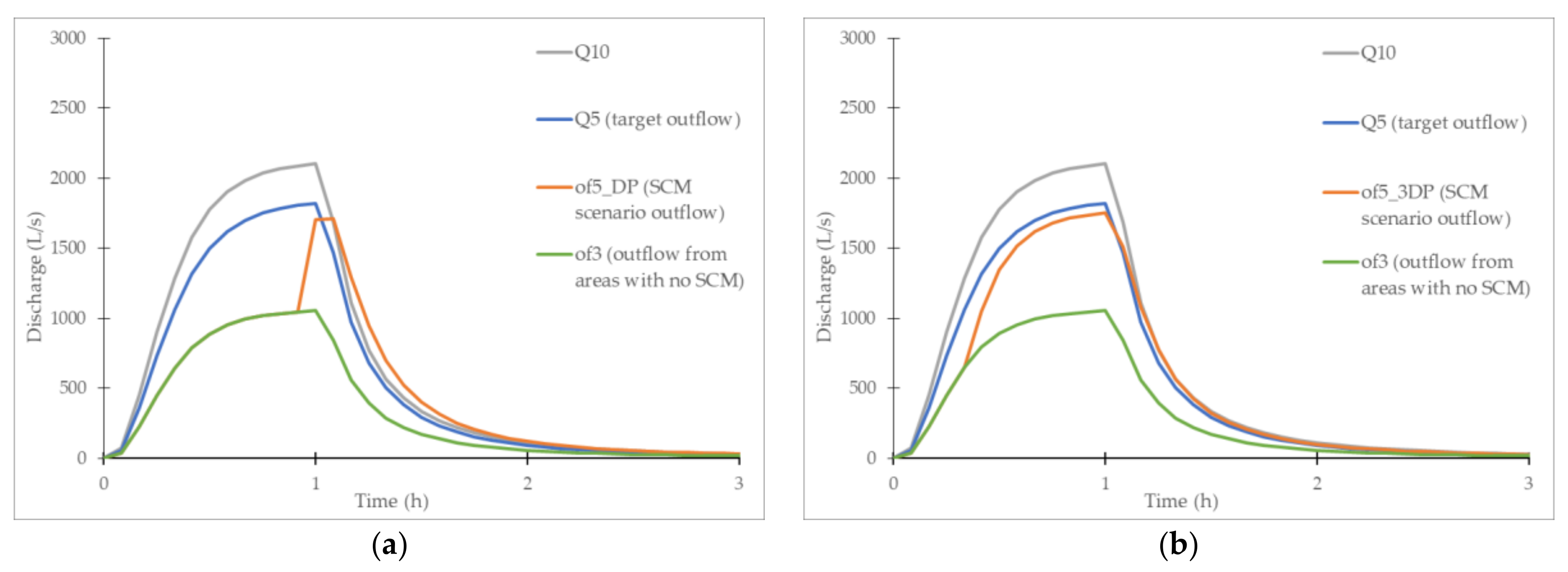
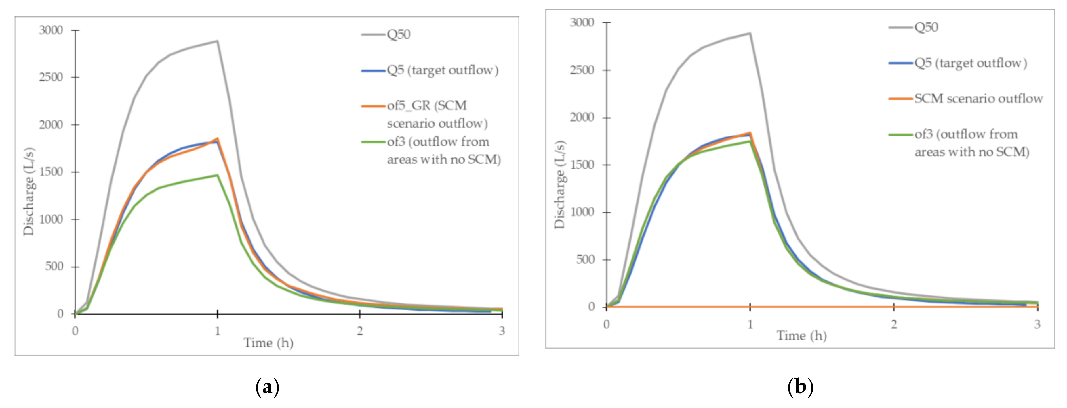
In the first round of SCM design, the conceptual model with three sub-compartments (Figure 4) was used. Furthermore, the surface area of all SCMs was set to 5000 m2, except for GR where this value was set to 50% of all the impervious area (i.e., 90,000 m2). The results showed that, in many cases, an SCM with uniform characteristics could not sufficiently follow the event dynamics. Namely, DPs and STs provide detention for a limited amount of time after which the outflow from SCM appears (Figure 5a). Therefore, the initial SCM sub-compartment (i.e., sub3), was further divided into three equally sized sub-compartments with SCMs (i.e., sub 3–5) (Figure 5b), enabling the design of three elements of the same SCM type with different characteristics (e.g., dimensions). Moreover, the initial simulation provided information on which SCMs could take up less space (i.e., shallow elements) (e.g., ST, DP, IF) or would need more space for its implementation (i.e., thick elements or significant overflow) (e.g., RG, BRC). Taking into account the above-mentioned observations, the following results were obtained.
3.2.1. Detention Pond and Storage Tank
Due to their similarity, detention ponds (DPs) and storage tanks (STs) provided comparable results. Namely, a near-perfect match between the target and simulated outflow was achieved for both measures (i.e., an NSE value of 0.99) (Appendix A Table A2 and Table A3). In the second round of SCM design, the areas of ST and DP were reduced by 80% (i.e., to total an SCM area of approximately 1000 m2). Thus, these are the two most space-efficient measures. As expected, larger and deeper elements were designed for less frequent design events and vice versa. In general, the measures can be divided into those that detain all the inflow from contributing areas, and those that provide outflow. For the latter, at least one of the dimensions was set to (or very close to) the minimum value (i.e., area to 250 m2 or depth to 0.5 m).
3.2.2. Infiltration Trench
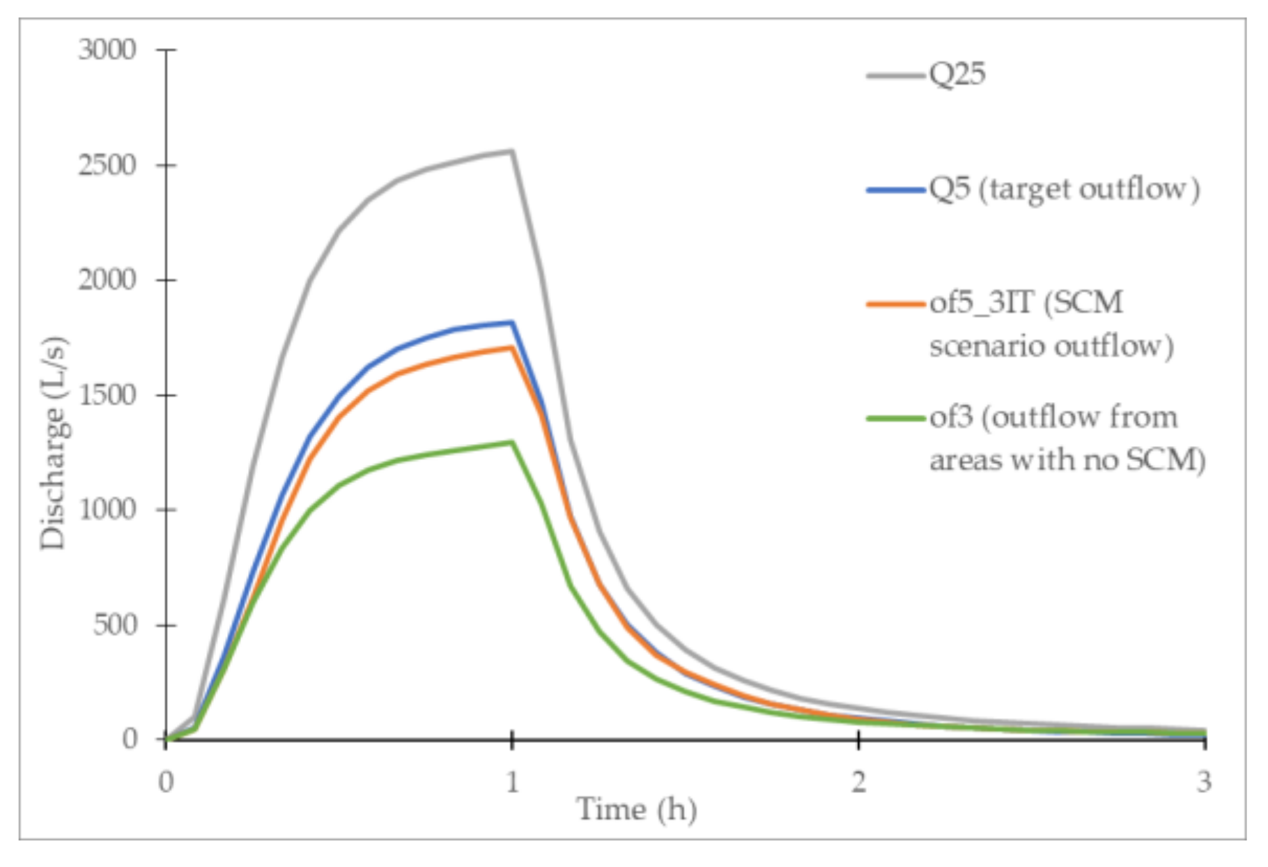
Infiltration trenches (ITs) also achieved a good fit between the target and simulated outflow (i.e., NSE value of 0.99) (Appendix A Table A4). However, when compared to ST and DP, these elements on average take 2.5 times more space (i.e., between 1997 and 3000 m2). This is caused by a smaller maximum depth (i.e., 3.5 m), smaller maximum voids fraction (i.e., 40%) and limited infiltration rate of the existing soil (i.e., m/s). On the other hand, IT can be implemented as a set of elements with tailor-made shapes, based on site conditions (e.g., along a plot border). As expected, larger and deeper elements were designed for less frequent design events and vice versa. For the design event DE_Q5_P25 (Figure 6), two ITs were designed to capture the whole run-off from contributing areas with the maximum area of 1.000 m2 and storage layer depths of 3.40 m and 2.62 m. The third IT (i.e., sub4) was designed using the min. dimensions (i.e., area 500 m2, 0 m of freeboard (i.e., D1) and a storage layer that is 0.9 m deep). Although the freeboard is set to 0 m, surface ponding can still occur. In this case, the maximum ponding depth (i.e., d1) is 0.25 m, highlighting the fact that IT with an even smaller area could be designed. However, this could increase the ponding height unreasonably.
3.2.3. Rain Garden and Bio-Retention Cell
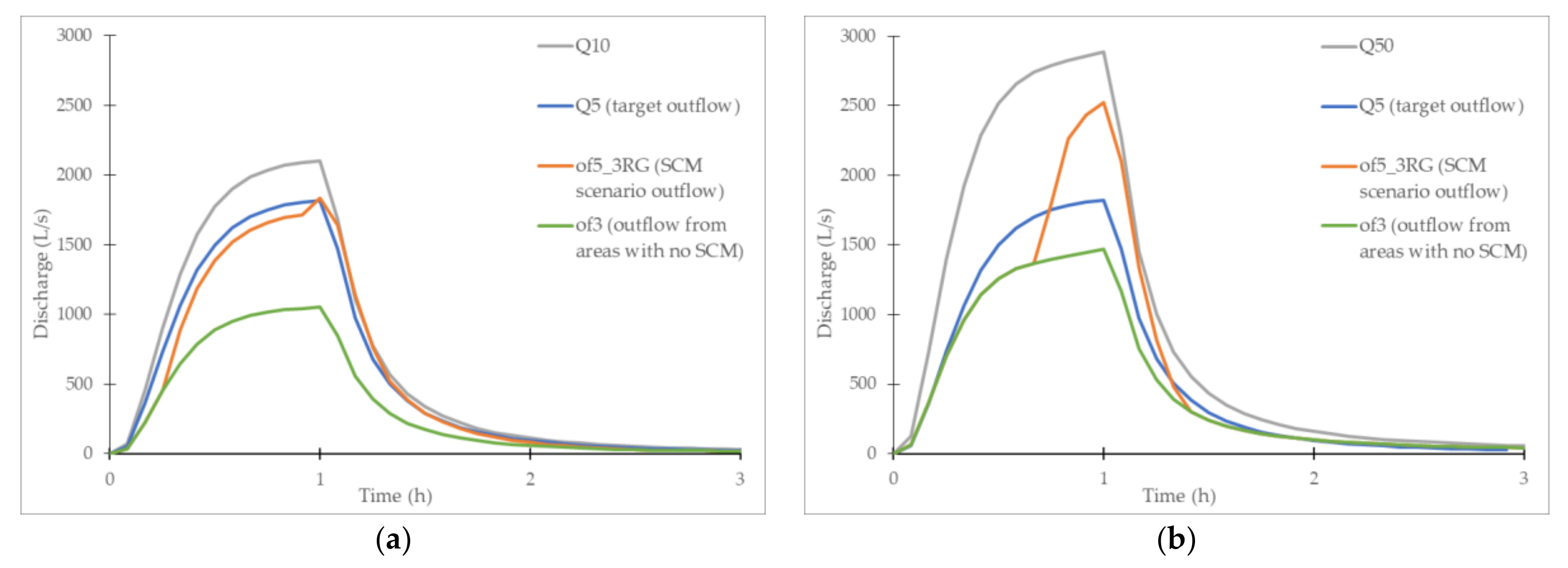
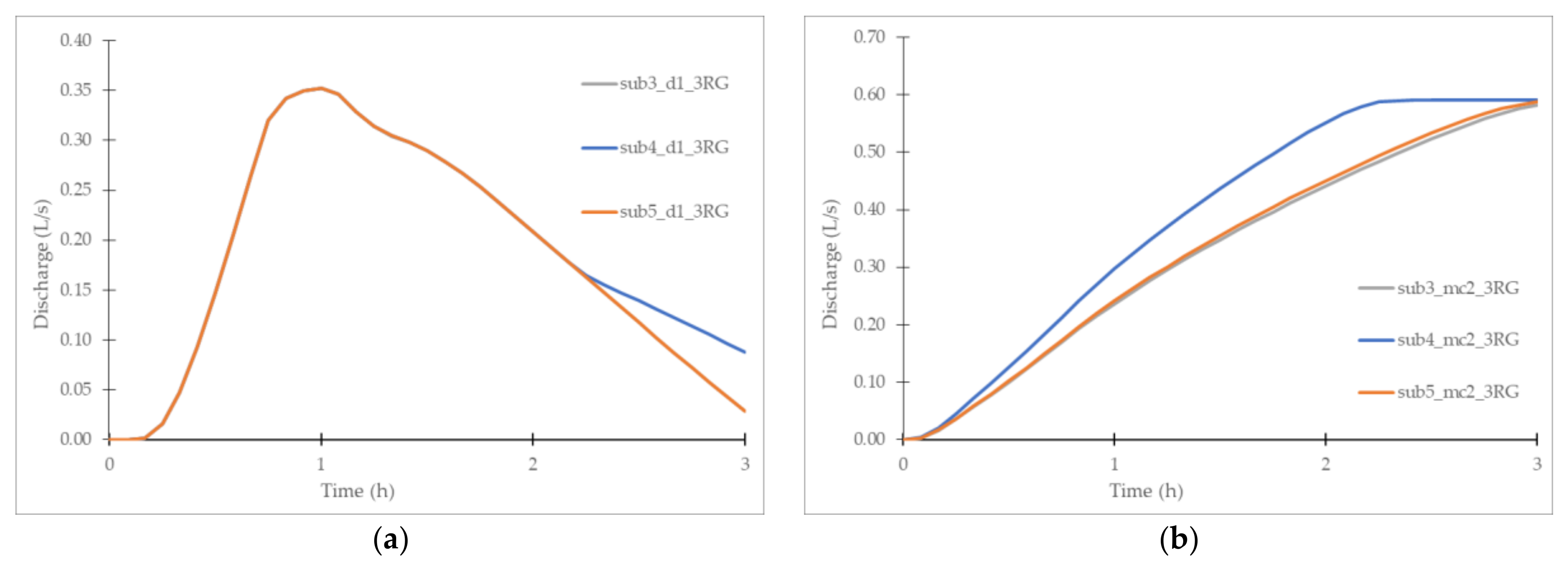
RGs and BRCs yielded similar results (Appendix A Table A5 and Table A6), as they are both limited by the soil infiltration rate (1), which is calculated based on the soil’s saturated hydraulic conductivity (K2S). Therefore, both measures performed well for DE_Q5_P10 (Figure 7a) but proved insufficient for DE_Q5_P50 (Figure 7b). Namely, although maximum parameter values, that would increase detention and infiltration, are selected for DE_Q5_P50, significant overflow occurs between the 45 and 75 the minute of simulation. This can be observed also in Figure 8a, where the overflow occurs when d1 exceeds the maximum freeboard (i.e., D1 is 0.30 m). As mentioned before, the infiltration rate is too low to transfer all the ponded water into the soil layer fast enough. Looking at Figure 8b, we can see that the soil layers’ moisture content riches maximum values (i.e., 0.60) only after 2 h. Among the SCMs that are placed within existing pervious areas, these two SCM types take up the most space, between 3000 and 6000 m2. However, in contrast to other SCMs that do not include a soil layer, they can offer additional ecosystem services (i.e., water filtration, biodiversity, etc.). It can be concluded that taking into account the proposed parameter values, including the SCM area, RGs and BRCs are more suitable measures for more frequent rain events (i.e., DE_Q5_P10).
3.2.4. Green Roof
In comparison to other SCMs, the green roof (GR) acts as a contributing area and an SCM area at the same time. Namely, it does not receive surface runoff (q0) from adjacent areas. GRs are a replacement for conventional roofs that act as impervious areas (i.e., sub1). Therefore, changes in the GR area have a direct influence on the size of the impervious area within sub1. Namely, if the GR area is increased, the impervious area has to be decreased by the same amount. Simulations showed that GRs could sufficiently detain all direct rainfall. Thus, the optimal GR area depends on the outflow from impervious (i.e., sub1) and pervious areas (i.e., sub2), which is in direct correlation with their size. Figure 9a presents results for DE_Q5_P50, where GRs replace 50% of existing impervious areas (i.e., 90,000 m2), resulting in an outflow from impervious and pervious areas (i.e., of3) that is lower than the target outflow (i.e., Q5). Consequently, GRs are designed in a way that they provide additional outflow (i.e., from sub4). As this design is suboptimal, the area of GRs was further reduced to 40% of existing impervious areas (i.e., 72,000 m2) (Appendix A Table A7). The results for this scenario show that only a small outflow from GRs occurs and that of3 almost matches the target outflow (i.e., Q5) (Figure 9b). For both design events of higher frequencies, the of3 was lower than the target outflow (i.e., Q5). Thus, the GRs were designed in a way to provide additional outflow.
3.2.5. Stormwater Control Measures Performance
In general, all of the SCM scenarios performed well, except for the scenarios 3RG and 3BRC, which exceeded the target peak flow, for the design events DE_Q5_P25 and DE_Q5_P50 (Table 7). As mentioned before, RGs and BRCs were limited by their design characteristics (e.g., soil’s saturated hydraulic conductivity) and the proposed area for implementation (i.e., 5% of the pervious area). If the additional area was available, these two scenarios could also perform well. Scenarios 3ST, 3DP, and 3IT slightly exceed the target outflow values for the design event DE_Q5_P50; however, they remain within tolerable limits. In this way, an optimal SCM design is provided, by setting some of the characteristics of the elements to the maximum possible value (e.g., depth of the surface layer, area …). The 3GR scenario, assuming that 40% of the current impervious areas will be replaced with green roofs, achieved the best performance.
4. Discussion
4.1. Rainfall-Runoff Models
The development of a validated RR model is a prerequisite for the assessment of hydrologic effectiveness of different SCM scenarios [25]. In this study, an automated equation (model) discovery approach that enabled the automatic generation and calibration of RR models was applied. The derived RR models can be classified as lumped (regarding spatial resolution) and continuous (regarding temporal resolution) [47]. To build fully distributed models, hydraulic processes (i.e., pipe flow) should be included. Due to some limitations of the ProBMoT tool, only hydrological processes were included. Hydraulic (pipe flow) modeling is crucial when modeling complex and large sewer system. In our case, the case study area and the adjacent sewer system were relatively small, thus the hydraulic (pipe flow) modeling would not significantly affect the outflow dynamics.
The developed knowledge library, compliant with the ProBMoT tool, enabled a systematic comparison of three alternative infiltration methods (i.e., SCS CN, VARUK, and UKWIR) and their combinations. This is a unique and novel approach, as normally only one infiltration method is used within one RR model [20].
In general, all RR models were judged to have »very good« performance, with only minor differences across models. Thus, no general conclusion can be made on which model is better, since model performance results are greatly influenced by the characteristics of calibration and validation periods (e.g., rainfall intensity, number of (sub) rainfall events) [46]. However, two of the models that combine infiltration methods performed best (i.e., M3, M4), highlighting the true value and contribution of this research, which is the discovery of new knowledge in the urban runoff-modeling domain by automated modeling.
In contrast to traditional machine learning methods for knowledge and model discovery that are purely data-driven, ProBMoT allows for integrating expert background knowledge from the domain of use in the process of equation/model discovery. The knowledge library, presented in this paper, provides a blueprint for building mechanistic, transparent models of hydrological events as opposed to black-box models that would be obtained by traditional data-driven methods. The blueprint results in a small number of candidate model structures, which significantly reduces the danger of overfitting the model to calibration (i.e., training) data. This robustness to overfitting explains why the resulting models often perform better on validation data and confirms the model generality, i.e., its ability to properly explain unobserved hydrological events and accurately predict their outcomes and implications.
We should distinguish between two major types of users of the proposed approach. The first type of users are domain experts and experienced users, who have a thorough understanding of the underlying physics. These users are allowed to create and modify libraries of domain knowledge, which include templates for modeling different processes that are consistent with the physics of the domain. The second type of users are so-called end-users. They can use libraries of domain knowledge, conceptual models, and measured data to solve specific urban catchment modeling and SCM design problems. Assuming that they lack in-depth knowledge of the underlying physics, they would not be allowed to modify the libraries of domain knowledge and the template formulas for modeling different processes.
4.2. Stormwater Control Measures
In this study, SCMs were designed based on the target catchment outflow (i.e., hydrograph). This is typical for auto-calibration of SCMs, where an objective function has to be defined [25]. Otherwise, the performance of SCMs is usually evaluated only with hydrological parameters (e.g., peak flow reduction, total volume) after their predetermined design and model simulation [4,16,19]. The hydrograph-based SCM design can be extremely helpful in situations where not only the peak flow is a limitation, but also the flow distribution (i.e., downstream convergence of outflows from catchments with different dynamics). In this way, this approach can be used to design SCMs and investigate to what extent they can reduce flood hazards. Moreover, in this study, all relevant SCMs parameters were included in the calibration (i.e., design) process, including material characteristics, as opposed to a more typical approach, where only a search for the optimal SCMs dimensions (e.g., surface) is conducted. A comparative analysis with other studies of the obtained SCM performance results cannot be conducted, due to different ratios between the contributing and the SCM area, the difference in implementation surface among SCM types, and specific local conditions.
5. Conclusions
In this study, an automated equation (model) discovery approach was applied to the field of RR modeling and SCM design. First, a new library of model components, compliant with the equation discovery tool ProBMoT was developed, formalizing the knowledge on RR modeling and SCM design. Next, a conceptual model of the experimental urban sub-catchment within the city of Ljubljana, Slovenia, was defined. The proposed automated model discovery approach was used to find the optimal structure among the viable RR models, based on pipe flow measurements.
The best RR model was used to simulate catchment outflow for rainfall events with a duration of 1 h and return periods of 5, 10, 25, and 50 years. The results were used to define three design events (i.e., data sets) that represent target catchment outflows. Namely, by using SCMs, the precipitation with a return period of 10, 25, or 50 years, should generate outflow typical for a 5-year return period. Next, ProBMoT was used to determine the optimal SCM parameters (i.e., SCM design), following the conceptual model for each SCM scenario and target catchment outflow (i.e., outflow reduction).
The main findings of the study are as follows:
- The proposed automated model discovery approach for finding the optimal RR models proved to be very efficient. Nine RR models were considered that generally had »very good« performance. The best performance was achieved by two models that used a combination of two different infiltration methods;
- The proposed automated model discovery approach enabled the design of six SCM scenarios and the assessment of their ability to achieve the target outflow;
- Detention ponds (DPs) and storage tanks (STs) provided comparable results. Namely, a near-perfect match between the target and simulated outflow was achieved for both measures (i.e., NSE value of 0.99). These are the two most space-efficient measures, with an average area of approx. 1000 m2);
- Infiltration trenches (ITs) achieved a good fit between the target and simulated outflow (i.e., NSE value of 0.99). When compared to ST and DP, these elements on average take 2.5 times more space, due to smaller maximum depth, smaller maximum voids fraction and limited infiltration rate of the existing soil;
- RGs and BRCs provided similar results, as they are both limited by the soil’s saturated hydraulic conductivity (i.e., parameter K2S). Therefore, both measures performed well only for the design event with the lowest intensity. Among the SCMs that are placed within existing pervious areas, these two SCM types take up the most space;
- The changes in the GR area have a direct influence on the size of the impervious area. Thus, the optimal GR area depends on the outflow from impervious and pervious areas. The outflow from impervious and pervious areas for the design event with a return period of 50 years almost matches the target outflow (i.e., Q5), if GRs replaced 40% of existing impervious areas.
Finally, this approach is transferable to any catchment and enables the discovery of viable RR models and target-based SCM design. To do so, the user has to specify a conceptual model of the selected case study area, compliant with the knowledge library. Furthermore, the user has to provide rainfall and flow measurement data and catchment characteristics (i.e., land use, topography, soil properties), based on which the values of the model constants can be determined.
The currently defined knowledge library encompasses knowledge defined in SWMM, but it is not limited to it. Namely, it can be further developed and upgraded with new SCM elements, equations, and parameters. Thus, it can serve as an open and flexible vehicle for testing new functionalities. In future research, a search among scenarios that integrate multiple SCMs can be conducted. Furthermore, the automated design of SCMs can be based on additional criteria (i.e., investment costs, biodiversity) that can be included within new objective functions.
Supplementary Materials
The following are available online at https://www.mdpi.com/article/10.3390/w13162268/s1, S1: Knowledge library, S2: Conceptual model.
Author Contributions
N.A. and M.R. conceptualized the research problem and formulated the goals, aims, and methodology of the study; M.R. collected and analyzed the flow measurement and precipitation data; M.R. developed a new knowledge library, formalizing the knowledge on RR modeling and SCM design, and conceptual models; M.R. investigated the effectiveness of the proposed approach on the case study area and conducted results visualization; S.D., L.T., and M.Š. supervised the application of the equation discovery tool ProBMoT; All authors contributed to the interpretation of the results, manuscript writing, and revision. All authors have read and agreed to the published version of the manuscript.
Funding
This work was supported by the Slovenian Research Agency (research core funding No. P2-0180, No. P2-0103, No. P5-0093, and project No. N2-0128).
Acknowledgments
The authors would like to thank the company JP VOKA SNAGA for providing the sewer system data and the Slovenian Forestry Institute for providing the precipitation data.
Conflicts of Interest
The authors declare no conflict of interest.
Appendix A

Table A1.
The considered rainfall-runoff model structures with the calibrated values of their parameters.
Table A1.
The considered rainfall-runoff model structures with the calibrated values of their parameters.
| M1 | M2 | M3 | M4 | M5 | M6 | M7 | M8 | M9 | ||||||||||
|---|---|---|---|---|---|---|---|---|---|---|---|---|---|---|---|---|---|---|
| sub1 | sub2 | sub1 | sub2 | sub1 | sub2 | sub1 | sub2 | sub1 | sub2 | sub1 | sub2 | sub1 | sub2 | sub1 | sub2 | sub1 | sub2 | |
| SCS CN | SCS CN | UKWIR | SCS CN | VARUK | SCS CN | SCS CN | UKWIR | UKWIR | UKWIR | VARUK | UKWIR | SCS CN | VARUK | UKWIR | VARUK | VARUK | VARUK | |
| A | 180,000 | 120,000 | 180,000 | 120,000 | 180,000 | 120,000 | 180,000 | 120,000 | 180,000 | 120,000 | 180,000 | 120,000 | 180,000 | 120,000 | 180,000 | 120,000 | 180,000 | 120,000 |
| S | 0.002 | 0.002 | 0.002 | 0.002 | 0.002 | 0.002 | 0.002 | 0.002 | 0.002 | 0.002 | 0.002 | 0.002 | 0.002 | 0.002 | 0.002 | 0.002 | 0.002 | 0.002 |
| W | 6092 | 3538 | 6083 | 5857 | 6000 | 5016 | 6000 | 3000 | 6033 | 6000 | 6141 | 6000 | 6112 | 3991 | 6103 | 5537 | 6164 | 6000 |
| ds | 0.0001 | 0.0060 | 0.0002 | 0.0005 | 0.0002 | 0.0048 | 0.0001 | 0.0060 | 0.0002 | 0.0026 | 0.0002 | 0.0014 | 0.0001 | 0.0005 | 0.0002 | 0.0018 | 0.0001 | 0.0017 |
| n | 0.08 | 0.67 | 0.08 | 0.15 | 0.08 | 0.75 | 0.08 | 0.25 | 0.08 | 0.15 | 0.08 | 0.15 | 0.08 | 0.26 | 0.08 | 0.15 | 0.08 | 0.18 |
| CN | 99 | 50 | null | 56 | null | 50 | 99 | null | null | null | null | null | 99 | null | null | null | null | null |
| PIMP | 100 | 0 | 100 | 0 | 100 | 0 | 100 | 0 | 100 | 0 | 100 | 0 | 100 | 0 | 100 | 0 | 100 | 0 |
| IF | null | null | 0.90 | null | 0.85 | null | null | 0.75 | 0.83 | 0.78 | 0.81 | 0.90 | null | 0.75 | 0.88 | 0.83 | 0.83 | 0.76 |
| B | null | null | 0.72 | null | null | null | null | 0.77 | 0.69 | 0.50 | null | 0.74 | null | null | 0.50 | null | null | null |
| PIimp | null | null | 1.00 | null | null | null | null | 1.00 | 1.00 | 0.42 | null | 1.00 | null | null | 0.64 | null | null | null |
| PFimp | null | null | 11.16 | null | null | null | null | 11.70 | 13.02 | 10.00 | null | 12.62 | null | null | 12.20 | null | null | null |
| NAPI | null | null | 17.36 | null | 25.00 | null | null | 12.11 | 14.97 | 27.55 | 30.00 | 26.94 | null | 12.91 | 30.00 | 30.00 | 12.00 | 30.00 |
| PIp | null | null | 0.90 | null | null | null | null | 0.88 | 0.75 | 0.74 | null | 0.77 | null | null | 0.70 | null | null | null |
| Cr | null | null | 1.00 | null | null | null | null | 0.80 | 0.98 | 0.86 | null | 0.85 | null | null | 0.82 | null | null | null |
| SPR | null | null | 0.35 | null | null | null | null | 0.68 | 0.10 | 0.66 | null | 0.56 | null | null | 0.70 | null | null | null |
| PFp | null | null | 58.25 | null | 32.35 | null | null | 30.00 | 100.00 | 30.00 | 60.96 | 42.27 | null | 100.00 | 100.00 | 100.00 | 50.74 | 100.00 |
Table A2.
The results of the 3ST scenario, which includes three types of a storage tank.
| 3ST | Results | ||||||
|---|---|---|---|---|---|---|---|
| A | D1 | NSE | TVR | PFR | |||
| Design event | DE_Q5_P10 | Sub3 | 250 | 0.50 | 0.97 | 0.94 | 0.96 |
| Sub4 | 364 | 4.70 | |||||
| Sub5 | 250 | 0.50 | |||||
| DE_Q5_P25 | Sub3 | 431 | 4.93 | 0.99 | 0.95 | 0.94 | |
| Sub4 | 499 | 3.99 | |||||
| Sub5 | 250 | 0.50 | |||||
| DE_Q5_P50 | Sub3 | 408 | 0.53 | 0.99 | 1.07 | 1.07 | |
| Sub4 | 462 | 5.00 | |||||
| Sub5 | 500 | 4.84 | |||||
Table A3.
The results of the 3DP scenario, which includes three types of a detention pond.
| 3DP | Results | ||||||
|---|---|---|---|---|---|---|---|
| A | D1 | NSE | TVR | PFR | |||
| Design event | DE_Q5_P10 | Sub3 | 101 | 0.50 | 0.97 | 0.94 | 0.96 |
| Sub4 | 100 | 0.50 | |||||
| Sub5 | 500 | 5.00 | |||||
| DE_Q5_P25 | Sub3 | 497 | 4.89 | 0.99 | 0.95 | 0.94 | |
| Sub4 | 100 | 0.50 | |||||
| Sub5 | 500 | 5.00 | |||||
| DE_Q5_P50 | Sub3 | 471 | 4.90 | 0.99 | 1.07 | 1.07 | |
| Sub4 | 391 | 5.00 | |||||
| Sub5 | 100 | 2.16 | |||||
Table A4.
The results of the 3IT scenario, which includes three types of an infiltration trench.
| 3IT | Results | ||||||||||
|---|---|---|---|---|---|---|---|---|---|---|---|
| A | D1 | D3 | VF1 | VF3 | K3S | NSE | TVR | PFR | |||
| Design event | DE_Q5_P10 | Sub3 | 983 | 0.26 | 3.50 | 1.00 | 0.39 | 2.6 × 10⁻⁵ | 0.98 | 0.92 | 0.95 |
| Sub4 | 100 | 0.00 | 0.90 | 1.00 | 0.20 | 2.6 × 10⁻⁵ | |||||
| Sub5 | 100 | 0.00 | 0.90 | 1.00 | 0.20 | 2.6 × 10⁻⁵ | |||||
| DE_Q5_P25 | Sub3 | 979 | 0.16 | 3.15 | 1.00 | 0.40 | 2.6 × 10⁻⁵ | 0.99 | 0.94 | 0.94 | |
| Sub4 | 100 | 0.00 | 0.90 | 1.00 | 0.20 | 2.6 × 10⁻⁵ | |||||
| Sub5 | 977 | 0.28 | 2.92 | 1.00 | 0.39 | 2.6 × 10⁻⁵ | |||||
| DE_Q5_P50 | Sub3 | 964 | 0.30 | 3.42 | 1.00 | 0.40 | 2.6 × 10⁻⁵ | 0.99 | 1.05 | 1.06 | |
| Sub4 | 951 | 0.29 | 3.50 | 1.00 | 0.39 | 2.6 × 10⁻⁵ | |||||
| Sub5 | 1000 | 0.00 | 1.01 | 1.00 | 0.21 | 2.6 × 10⁻⁵ | |||||
Table A5.
The results of the 3RG scenario, which includes three types of a rain garden.
| 3RG | Results | |||||||||||||||||||
|---|---|---|---|---|---|---|---|---|---|---|---|---|---|---|---|---|---|---|---|---|
| A | D1 | D2 | D3 | VF1 | VF2 | VF3 | K2S | K3S | SH2 | HCO | IMC2 | FC | af_max | af_k | NSE | TVR | PFR | |||
| Design event | DE_Q5_P10 | Sub3 | 500 | 0.10 | 0.77 | null | 0.80 | 0.45 | null | 1.4 × 10⁻⁵ | 2.6 × 10⁻⁵ | 0.05 | 39.3 | 0.08 | 0.15 | 1.0 | 0.001 | 0.98 | 0.95 | 1.01 |
| Sub4 | 500 | 0.10 | 0.87 | null | 0.80 | 0.45 | null | 1.4 × 10⁻⁵ | 2.6 × 10⁻⁵ | 0.05 | 39.3 | 0.08 | 0.15 | 1.0 | 0.001 | |||||
| Sub5 | 2000 | 0.30 | 1.02 | null | 0.80 | 0.60 | null | 3.9 × 10⁻⁵ | 2.6 × 10⁻⁵ | 0.05 | 39.3 | 0.08 | 0.15 | 1.0 | 0.001 | |||||
| DE_Q5_P25 | Sub3 | 743 | 0.10 | 0.60 | null | 0.80 | 0.50 | null | 3.9 × 10⁻⁵ | 2.6 × 10⁻⁵ | 0.05 | 39.3 | 0.08 | 0.15 | 1.0 | 0.001 | 0.96 | 1.03 | 1.24 | |
| Sub4 | 2000 | 0.30 | 0.68 | null | 0.80 | 0.60 | null | 3.9 × 10⁻⁵ | 2.6 × 10⁻⁵ | 0.05 | 39.3 | 0.08 | 0.15 | 1.0 | 0.001 | |||||
| Sub5 | 2000 | 0.30 | 1.20 | null | 0.80 | 0.60 | null | 3.9 × 10⁻⁵ | 2.6 × 10⁻⁵ | 0.05 | 39.3 | 0.08 | 0.15 | 1.0 | 0.001 | |||||
| DE_Q5_P50 | Sub3 | 2000 | 0.30 | 1.03 | null | 0.80 | 0.60 | null | 3.9 × 10⁻⁵ | 2.6 × 10⁻⁵ | 0.05 | 39.3 | 0.08 | 0.15 | 1.0 | 0.001 | 0.87 | 1.08 | 1.38 | |
| Sub4 | 2000 | 0.30 | 0.82 | null | 0.80 | 0.60 | null | 3.9 × 10⁻⁵ | 2.6 × 10⁻⁵ | 0.05 | 39.3 | 0.08 | 0.15 | 1.0 | 0.001 | |||||
| Sub5 | 2000 | 0.30 | 1.01 | null | 0.80 | 0.60 | null | 3.9 × 10⁻⁵ | 2.6 × 10⁻⁵ | 0.05 | 39.3 | 0.08 | 0.15 | 1.0 | 0.001 | |||||
Table A6.
The results of the 3BRC scenario, which includes three types of a bio-retention cell.
| 3BRC | Results | |||||||||||||||||||
|---|---|---|---|---|---|---|---|---|---|---|---|---|---|---|---|---|---|---|---|---|
| A | D1 | D2 | D3 | VF1 | VF2 | VF3 | K2S | K3S | SH2 | HCO | IMC2 | FC | af_max | af_k | NSE | TVR | PFR | |||
| Design event | DE_Q5_P10 | Sub3 | 500 | 0.10 | 0.60 | 0.15 | 0.80 | 0.45 | 0.23 | 1.4 × 10⁻⁵ | 2.6 × 10⁻⁵ | 0.05 | 39.3 | 0.08 | 0.15 | 1.0 | 0.001 | 0.99 | 0.93 | 0.95 |
| Sub4 | 500 | 0.10 | 0.63 | 0.90 | 0.80 | 0.45 | 0.20 | 1.4 × 10⁻⁵ | 2.6 × 10⁻⁵ | 0.05 | 39.3 | 0.08 | 0.15 | 1.0 | 0.001 | |||||
| Sub5 | 2000 | 0.30 | 0.69 | 0.90 | 1.00 | 0.60 | 0.26 | 3.9 × 10⁻⁵ | 2.6 × 10⁻⁵ | 0.05 | 39.3 | 0.08 | 0.15 | 1.0 | 0.001 | |||||
| DE_Q5_P25 | Sub3 | 500 | 0.10 | 0.69 | 0.90 | 0.80 | 0.45 | 0.29 | 3.9 × 10⁻⁵ | 2.6 × 10⁻⁵ | 0.05 | 39.3 | 0.08 | 0.15 | 1.0 | 0.001 | 0.97 | 1.01 | 1.17 | |
| Sub4 | 2000 | 0.30 | 0.76 | 0.30 | 1.00 | 0.60 | 0.40 | 3.9 × 10⁻⁵ | 2.6 × 10⁻⁵ | 0.05 | 39.3 | 0.08 | 0.15 | 1.0 | 0.001 | |||||
| Sub5 | 2000 | 0.30 | 1.15 | 0.90 | 1.00 | 0.60 | 0.23 | 3.9 × 10⁻⁵ | 2.6 × 10⁻⁵ | 0.05 | 39.3 | 0.08 | 0.15 | 1.0 | 0.001 | |||||
| DE_Q5_P50 | Sub3 | 2000 | 0.12 | 0.66 | 0.27 | 0.80 | 0.60 | 0.37 | 3.9 × 10⁻⁵ | 2.6 × 10⁻⁵ | 0.05 | 39.3 | 0.08 | 0.15 | 1.0 | 0.001 | 0.91 | 1.10 | 1.37 | |
| Sub4 | 2000 | 0.30 | 0.88 | 0.65 | 1.00 | 0.60 | 0.36 | 3.9 × 10⁻⁵ | 2.6 × 10⁻⁵ | 0.05 | 39.3 | 0.08 | 0.15 | 1.0 | 0.001 | |||||
| Sub5 | 2000 | 0.30 | 0.94 | 0.46 | 1.00 | 0.60 | 0.40 | 3.9 × 10⁻⁵ | 2.6 × 10⁻⁵ | 0.05 | 39.3 | 0.08 | 0.15 | 1.0 | 0.001 | |||||
Table A7.
The results of the 3GR scenario, which includes three types of a green roof.
| 3GR | Results | |||||||||||||||||||||||
|---|---|---|---|---|---|---|---|---|---|---|---|---|---|---|---|---|---|---|---|---|---|---|---|---|
| A | width | slope | n1 | n3 | D1 | D2 | D3 | VF1 | VF2 | VF3 | K2S | K3S | SH2 | HCO | IMC2 | FC | af_max | af_k | NSE | TVR | PFR | |||
| Design event | DE_Q5_P10 | Sub3 | 24,000 | 2400 | 0.02 | 0.180 | 0.023 | 0.000 | 0.050 | 0.050 | 0.99 | 0.45 | 0.40 | 3 × 10⁻⁶ | null | 0.05 | 39.3 | 0.08 | 0.15 | 1.0 | 0.001 | 1.00 | 0.99 | 1.02 |
| Sub4 | 24,000 | 2400 | 0.02 | 0.174 | 0.020 | 0.000 | 0.050 | 0.019 | 0.99 | 0.45 | 0.40 | 3 × 10⁻⁶ | null | 0.05 | 39.3 | 0.08 | 0.15 | 1.0 | 0.001 | |||||
| Sub5 | 24,000 | 2400 | 0.02 | 0.188 | 0.019 | 0.000 | 0.050 | 0.013 | 1.00 | 0.45 | 0.34 | 3 × 10⁻⁶ | null | 0.05 | 39.3 | 0.08 | 0.15 | 1.0 | 0.001 | |||||
| DE_Q5_P25 | Sub3 | 24,000 | 2400 | 0.02 | 0.206 | 0.020 | 0.066 | 0.142 | 0.041 | 0.87 | 0.60 | 0.21 | 3 × 10⁻⁶ | null | 0.05 | 39.3 | 0.08 | 0.15 | 1.0 | 0.001 | 1.00 | 1.00 | 1.02 | |
| Sub4 | 24,000 | 2400 | 0.02 | 0.400 | 0.010 | 0.000 | 0.050 | 0.010 | 1.00 | 0.45 | 0.20 | 3 × 10⁻⁶ | null | 0.05 | 39.3 | 0.08 | 0.15 | 1.0 | 0.001 | |||||
| Sub5 | 24,000 | 2400 | 0.02 | 0.149 | 0.010 | 0.068 | 0.144 | 0.035 | 0.80 | 0.58 | 0.20 | 3 × 10⁻⁶ | null | 0.05 | 39.3 | 0.08 | 0.15 | 1.0 | 0.001 | |||||
| DE_Q5_P50 | Sub3 | 24,000 | 2400 | 0.02 | 0.242 | 0.015 | 0.003 | 0.141 | 0.036 | 1.00 | 0.54 | 0.20 | 3 × 10⁻⁶ | null | 0.05 | 39.3 | 0.08 | 0.15 | 1.0 | 0.001 | 1.00 | 1.01 | 1.001 | |
| Sub4 | 24,000 | 2400 | 0.02 | 0.304 | 0.030 | 0.036 | 0.139 | 0.026 | 0.87 | 0.60 | 0.24 | 3 × 10⁻⁶ | null | 0.05 | 39.3 | 0.08 | 0.15 | 1.0 | 0.001 | |||||
| Sub5 | 24,000 | 2400 | 0.02 | 0.102 | 0.030 | 0.073 | 0.137 | 0.011 | 0.88 | 0.60 | 0.30 | 3 × 10⁻⁶ | null | 0.05 | 39.3 | 0.08 | 0.15 | 1.0 | 0.001 | |||||
References
- Fletcher, T.D.; Shuster, W.; Hunt, W.F.; Ashley, R.; Butler, D.; Arthur, S.; Trowsdale, S.; Barraud, S.; Semadeni-Davies, A.; Bertrand-Krajewski, J.L.; et al. SUDS, LID, BMPs, WSUD and more—The evolution and application of terminology surrounding urban drainage. Urban Water J. 2015, 12, 525–542. [Google Scholar] [CrossRef]
- Versini, P.A.; Kotelnikova, N.; Poulhes, A.; Tchiguirinskaia, I.; Schertzer, D.; Leurent, F. A distributed modelling approach to assess the use of Blue and Green Infrastructures to fulfil stormwater management requirements. Landsc. Urban Plan. 2018, 173, 60–63. [Google Scholar] [CrossRef] [Green Version]
- Ellis, J.B.; Viavattene, C. Sustainable urban drainage system modeling for managing urban surface water flood risk. CLEAN Soil Air Water 2014, 42, 153–159. [Google Scholar] [CrossRef]
- Joshi, P.; Leitão, J.P.; Maurer, M.; Bach, P.M. Not all SuDS are created equal: Impact of different approaches on combined sewer overflows. Water Res. 2021, 191, 116780. [Google Scholar] [CrossRef]
- Zanin, G.; Bortolini, L. Performance of Three Different Native Plant Mixtures for Extensive Green Roofs in a Humid Subtropical Climate Context. Water 2020, 12, 3484. [Google Scholar] [CrossRef]
- Chen, X.; Peltier, E.; Sturm, B.S.M.; Young, C.B. Nitrogen removal and nitrifying and denitrifying bacteria quantification in a stormwater bioretention system. Water Res. 2013, 47, 1691–1700. [Google Scholar] [CrossRef]
- Petit-Boix, A.; Sevigné-Itoiz, E.; Rojas-Gutierrez, L.A.; Barbassa, A.P.; Josa, A.; Rieradevall, J.; Gabarrell, X. Environmental and economic assessment of a pilot stormwater infiltration system for flood prevention in Brazil. Ecol. Eng. 2015, 84, 194–201. [Google Scholar] [CrossRef] [Green Version]
- Alam, T.; Mahmoud, A.; Jones, K.D.; Bezares-Cruz, J.C.; Guerrero, J. A Comparison of Three Types of Permeable Pavements for Urban Runoff Mitigation in the Semi-Arid South Texas, U.S.A. Water 2019, 11, 1992. [Google Scholar] [CrossRef] [Green Version]
- Cannavo, P.; Coulon, A.; Charpentier, S.; Béchet, B.; Vidal-Beaudet, L. Water balance prediction in stormwater infiltration basins using 2-D modeling: An application to evaluate the clogging process. Int. J. Sediment Res. 2018, 33, 371–384. [Google Scholar] [CrossRef]
- Zhang, B.; Li, J.; Li, Y. Simulation and optimization of rain gardens via DRAINMOD model and response surface methodology. Ecohydrol. Hydrobiol. 2020, 20, 413–423. [Google Scholar] [CrossRef]
- Li, G.; Xiong, J.; Zhu, J.; Liu, Y.; Dzakpasu, M. Design influence and evaluation model of bioretention in rainwater treatment: A review. Sci. Total Environ. 2021, 787, 147592. [Google Scholar] [CrossRef]
- Yazdi, A.; Hamzehpour, H.; Sahimi, M. Permeability, porosity, and percolation of two-dimensional disordered fracture networks. Phys. Rev. E 2011, 84, 046347. [Google Scholar] [CrossRef]
- Parteli, E.J.R.; da Silva, L.R.; Andrade, J.S., Jr. Self-organized percolation in multi-layered structures. J. Stat. Mech. 2010, 46, P03023. [Google Scholar] [CrossRef] [Green Version]
- NRCS. Urban Hydrology for Small Watersheds TR-55; USDA: Washington, DC, USA, 1986. [Google Scholar]
- Rossman, L.A. Storm Water Management Model User’s Manual Version 5.1; United States Environmental Protection Agency: Washington, DC, USA, 2015; 353p. [Google Scholar]
- Li, Y.; Huang, J.J.; Hu, M.; Yang, H.; Tanaka, K. Design of low impact development in the urban context considering hydrological performance and life-cycle cost. J. Flood Risk Manag. 2020, 13, e12625. [Google Scholar] [CrossRef]
- Kong, F.; Ban, Y.; Yin, H.; James, P.; Dronova, I. Modeling stormwater management at the city district level in response to changes in land use and low impact development. Environ. Model. Softw. 2017, 95, 132–142. [Google Scholar] [CrossRef]
- Palla, A.; Gnecco, I. Hydrologic modeling of Low Impact Development systems at the urban catchment scale. J. Hydrol. 2015, 528, 361–368. [Google Scholar] [CrossRef]
- Chui, T.F.M.; Liu, X.; Zhan, W. Assessing cost-effectiveness of specific LID practice designs in response to large storm events. J. Hydrol. 2016, 533, 353–364. [Google Scholar] [CrossRef]
- Niazi, M.; Nietch, C.; Maghrebi, M.; Jackson, N.; Bennett, B.R.; Tryby, M.; Massoudieh, A. Storm Water Management Model: Performance Review and Gap Analysis. J. Sustain. Water Built Environ. 2017, 3, 04017002. [Google Scholar] [CrossRef] [Green Version]
- Hu, Y.; Scavia, D.; Kerkez, B. Are all data useful? Inferring causality to predict flows across sewer and drainage systems using directed information and boosted regression trees. Water Res. 2018, 145, 697–706. [Google Scholar] [CrossRef]
- Perin, R.; Trigatti, M.; Nicolini, M.; Campolo, M.; Goi, D. Automated calibration of the EPA-SWMM model for a small suburban catchment using PEST: A case study. Environ. Monit. Assess. 2020, 192, 374. [Google Scholar] [CrossRef]
- Koc, K.; Ekmekcioğlu, Ö.; Özger, M. An integrated framework for the comprehensive evaluation of low impact development strategies. J. Environ. Manag. 2021, 294, 113023. [Google Scholar] [CrossRef]
- Shahed Behrouz, M.; Zhu, Z.; Matott, L.S.; Rabideau, A.J. A new tool for automatic calibration of the Storm Water Management Model (SWMM). J. Hydrol. 2020, 581, 124436. [Google Scholar] [CrossRef]
- Zhu, Z.; Chen, Z.; Chen, X.; Yu, G. An assessment of the hydrologic effectiveness of low impact development (LID) practices for managing runoff with different objectives. J. Environ. Manag. 2019, 231, 504–514. [Google Scholar] [CrossRef]
- Doherty, J.; Hunt, R.; Tonkin, M. Approaches to highly parameterized inversion: A guide to using PEST for model-parameter and predictive-uncertainty analysis. US Geol. Surv. Sci. Investig. Rep. 2011, 2010, 71. [Google Scholar]
- Džeroski, S.; Todorovski, L. Equation discovery for systems biology: Finding the structure and dynamics of biological networks from time course data. Curr. Opin. Biotechnol. 2008, 19, 360–368. [Google Scholar] [CrossRef] [PubMed]
- Atanasova, N.; Todorovski, L.; Džeroski, S.; Kompare, B. Constructing a library of domain knowledge for automated modelling of aquatic ecosystems. Ecol. Modell. 2006, 194, 14–36. [Google Scholar] [CrossRef]
- Škerjanec, M.; Atanasova, N.; Čerepnalkoski, D.; Džeroski, S.; Kompare, B. Development of a knowledge library for automated watershed modeling. Environ. Model. Softw. 2014, 54, 60–72. [Google Scholar] [CrossRef]
- Tanevski, J.; Todorovski, L.; Džeroski, S. Process-based design of dynamical biological systems. Sci. Rep. 2016, 6, 34107. [Google Scholar] [CrossRef]
- Simidjievski, N.; Todorovski, L.; Kocijan, J.; Džeroski, S. Equation Discovery for Nonlinear System Identification. IEEE Access 2020, 8, 29930–29943. [Google Scholar] [CrossRef]
- Džeroski, S.; Todorovski, L.; Čerepnalkoski, D.; Tanevski, J.; Simidjievski, N. Process-Based Modeling Tool (ProBMoT). Available online: http://probmot.ijs.si/ (accessed on 7 January 2019).
- Slovenian Environment Agency. Temperature and Condition of Soil. Available online: http://meteo.arso.gov.si/met/sl/agromet/recent/tsoil (accessed on 5 July 2018).
- Slovenian Forestry Institute. Slovenian Forestry Institute Database of the Slovenian Forestry Institute 2018–2019; Web application eEMIS® 2019; Slovenian Forestry Institute: Ljubljana, Slovenia, 2019. [Google Scholar]
- Onset Computer Corporation Davis® (0.01′′ or 0.2 mm) Rain Gauge Smart Sensor (S-RGC-M002, S-RGD-M002) Manual. Available online: https://www.onsetcomp.com/files/manual_pdfs/19878-A%20MAN-S-RGCD.pdf (accessed on 18 June 2020).
- Slovenian Environment Agency IDF Curves—Ljubljana. Available online: https://meteo.arso.gov.si/uploads/probase/www/climate/table/sl/by_variable/return-periods/Ljubljana%20Bezigrad.pdf (accessed on 5 July 2018).
- Raven-Eye Non-Contact Radar Flow Measuring System. Available online: http://www.trilobit.si/files/2_Tec-Spec%20RAVEN-EYE%20EN.pdf (accessed on 18 August 2020).
- Mannina, G.; Viviani, G. An urban drainage stormwater quality model: Model development and uncertainty quantification. J. Hydrol. 2010, 381, 248–265. [Google Scholar] [CrossRef]
- Dai, Y.; Chen, L.; Shen, Z. A cellular automata (CA)-based method to improve the SWMM performance with scarce drainage data and its spatial scale effect. J. Hydrol. 2020, 581, 124402. [Google Scholar] [CrossRef]
- Butler, D.; Digman, C.J.; Makropoulos, C.; Davies, W.J. Urban Drainage, 4th ed.; Taylor & Francis e-Library: Boca Raton, FL, USA, 2018; ISBN 9788578110796. [Google Scholar]
- Packman, J.C. New hydrology model. In Proceedings of the WaPUG Conference, Glasgow, UK, 24 April 1990. [Google Scholar]
- Kellagher, R. A Guide to the Use of the UKWIR Runoff Equation; UK Water Industry Research: London, UK, 2014. [Google Scholar]
- Čerepnalkoski, D.; Taškova, K.; Todorovski, L.; Atanasova, N.; Džeroski, S. The influence of parameter fitting methods on model structure selection in automated modeling of aquatic ecosystems. Ecol. Modell. 2012, 245, 136–165. [Google Scholar] [CrossRef]
- Nash, J.E.; Sutcliffe, J.V. River flow forecasting through conceptual models part I—A discussion of principles. J. Hydrol. 1970, 10, 282–290. [Google Scholar] [CrossRef]
- Moriasi, D.N.; Arnold, J.G.; Van Liew, M.W.; Bingner, R.L.; Harmel, R.L.; Veith, T.L. Model Evaluation Guidelines for Systematic Quantification of Accuracy in Watershed Simulations. Trans. ASABE 2007, 50, 885–900. [Google Scholar] [CrossRef]
- Broekhuizen, I.; Leonhardt, G.; Marsalek, J.; Viklander, M. Event selection and two-stage approach for calibrating models of green urban drainage systems. Hydrol. Earth Syst. Sci. 2020, 24, 869–885. [Google Scholar] [CrossRef] [Green Version]
- Fletcher, T.D.; Andrieu, H.; Hamel, P. Understanding, management and modelling of urban hydrology and its consequences for receiving waters: A state of the art. Adv. Water Resour. 2013, 51, 261–279. [Google Scholar] [CrossRef]
Figure 1.
Case study area.

Figure 2.
A conceptual model of a typical bio-retention cell (adapted from [15]).
Figure 2.
A conceptual model of a typical bio-retention cell (adapted from [15]).

Figure 3.
A schematic workflow for the rainfall-runoff (RR) model discovery and stormwater control measure (SCM) design using the automated modeling tool ProBMoT.
Figure 3.
A schematic workflow for the rainfall-runoff (RR) model discovery and stormwater control measure (SCM) design using the automated modeling tool ProBMoT.

Figure 4.
Graphical representation of the development of the conceptual model structure that includes stormwater control measures (SCMs). (a) Initial conceptual model with two sub-compartments; (b) Introduction of SCM together with contributing area; (c) Final conceptual model including SCM consisting of three sub-compartments.

Figure 5.
The results of the DP scenario (a), which includes one type of a detention pond, and the 3DP scenario (b), which includes three types of a detention pond, for DE_Q5_P10.
Figure 5.
The results of the DP scenario (a), which includes one type of a detention pond, and the 3DP scenario (b), which includes three types of a detention pond, for DE_Q5_P10.

Figure 6.
The results of the 3IT scenario, which includes three types of an infiltration trench, for DE_Q5_P25.
Figure 6.
The results of the 3IT scenario, which includes three types of an infiltration trench, for DE_Q5_P25.

Figure 7.
The results of the 3RG scenario, which includes three types of a rain garden, for DE_Q5_P10 (a), and DE_Q5_P50 (b).
Figure 7.
The results of the 3RG scenario, which includes three types of a rain garden, for DE_Q5_P10 (a), and DE_Q5_P50 (b).

Figure 8.
The results of the 3RG scenario, which includes three types of a rain garden, for DE_Q5_P50: (a) depth of water stored on the surface (d1), and (b) soil layer moisture content (mc2).
Figure 8.
The results of the 3RG scenario, which includes three types of a rain garden, for DE_Q5_P50: (a) depth of water stored on the surface (d1), and (b) soil layer moisture content (mc2).

Figure 9.
The results of the 3GR scenario, which includes three types of green roofs, for DE_Q5_P50: (a) 3GR area 90,000 m2, and (b) 3GR area 72,000 m2.
Figure 9.
The results of the 3GR scenario, which includes three types of green roofs, for DE_Q5_P50: (a) 3GR area 90,000 m2, and (b) 3GR area 72,000 m2.

Table 1.
Characteristics of the selected rainfall periods used for calibration and validation.
| Period ID | Rainfall Period —Start | Rainfall Period —End | Duration (h) | Season | Total Precipitation (mm) | Total Precipitation Time (h) | Average Precipitation Intensity (mm/5 min) | Total Measured Flow (m3) | Measured Peak Flow (L/s) |
|---|---|---|---|---|---|---|---|---|---|
| C1_1D | 01.12.2019 (23:00) | 02.12.2019 (19:00) | 20 | Autumn | 24.4 | 8.3 | 0.24 | 8948 | 278 |
| C2_1D | 15.05.2020 (05:00) | 16.05.2020 (03:00) | 22 | Spring | 29.6 | 7.3 | 0.34 | 7409 | 442 |
| C3_6D | 23.04.2019 (04:30) | 29.04.2019 (04:30) | 144 | Spring | 39.8 | 13.6 | 0.24 | 6562 | 308 |
| C4_7D | 11.11.2019 (12:30) | 18.11.2019 (11:30) | 167 | Autumn | 74.4 | 25.3 | 0.25 | 20,938 | 555 |
| V1_1D | 31.08.2020 (12:00) | 01.09.2020 (11:00) | 23 | Summer | 20.8 | 7.8 | 0.22 | 5417 | 238 |
| V2_2D | 21.12.2019 (08:00) | 23.12.2019 (02:00) | 42 | Winter | 56.4 | 14.3 | 0.33 | 17.045 | 429 |
| V3_5D | 28.09.2019 (12:00) | 03.10.2019 (01:00) | 109 | Autumn | 38.8 | 8.5 | 0.38 | 7.854 | 283 |
| V4_5D | 01.03.2020 (07:00) | 06.03.2020 (15:00) | 128 | Winter | 81 | 26.1 | 0.26 | 19,578 | 301 |
Table 2.
Description of variables included in the rainfall-runoff model.
| Variables | |||
|---|---|---|---|
| SCS CN, VARUK, UKWIR Name | ProBMoT Name | Description | Unit |
| d | d | surface storage (ponded water) | m |
| i | i | rate of rainfall | m/s |
| f | f | infiltration rate | m/s |
| q | q | runoff flow rate per unit of surface area | m/s |
| * | cumulative infiltration at the beginning of a time step Δt | m | |
| * | cumulative infiltration at the end of a time step Δt | m | |
| F | * | cumulative infiltration | mm |
| P | p1, p2 | cumulative precipitation | mm |
| * | maximum storage capacity of soil | mm | |
| PR | * | percentage runoff for the model | |
* Variable is embedded as equation.
Table 3.
Description of constants included in the rainfall-runoff model, with assigned ranges for impervious and pervious areas (entity Surface).
Table 3.
Description of constants included in the rainfall-runoff model, with assigned ranges for impervious and pervious areas (entity Surface).
| Constants | |||||
|---|---|---|---|---|---|
| SCS CN, VARUK, UKWIR Name | ProBMoT Name | Description | Unit | Range | |
| IMP. | PERV. | ||||
| A | A | surface area of the sub-catchment | m2 | 180,000 | 120,000 |
| W | W | sub-catchment width | m | 6000–18,000 | 3000–6000 |
| S | S | average slope of the sub-catchment | m/m | 0.002 | 0.002 |
| ds | depression storage depth | m | 0.00005–0.001 | 0.0005–0.006 | |
| n | n | the surface roughness coefficient | 0.01–0.08 | 0.15–0.80 | |
| Δt | time step | s | 300 | 300 | |
| CN | CN | tabulated coefficient that varies with the land use and soil type | 90–99 | 30–75 | |
| PIMP | percentage of imperviousness | 100 | 0 | ||
| IF | effective impermeability factor for a particular paved surface type | 0.5–1 | / | ||
| β | B | power coefficient for a paved surface | 0.5–0.8 | / | |
| PIimp | precipitation index for paved surfaces with a rapid decay coefficient | 0–1 | / | ||
| PFimp | soil store depth for a paved surface | mm | 10–15 | / | |
| NAPI | antecedent precipitation index for a particular pervious surface type | mm | / | 0–40 | |
| PIp | precipitation index for pervious surface with a decay coefficient | / | 0.7–0.9 | ||
| Cr | Cr | power coefficient for pervious surface | / | 0.8–1.0 | |
| SPR | SPR | standard percentage runoff | / | 0.1–0.7 | |
| PFp | soil storage depth for a particular pervious surface type | mm | / | 30–50 | |
Table 4.
Variables used for stormwater control measures.
| Variables | |||
|---|---|---|---|
| EPA-SWMM Name | ProBMoT Name | Description | Unit |
| d1 | depth of water stored on the surface | m | |
| d3 | depth of water in the storage layer | m | |
| mc2 | soil layer moisture content (volume of water/total volume of soil) | fraction | |
| i | i | precipitation rate falling directly on the surface layer | m/s |
| q0 | inflow to the surface layer from runoff captured from other areas | m/s | |
| q1 | surface layer runoff or overflow rate | m/s | |
| f1 | infiltration rate of surface water into the soil layer | m/s | |
| f2 | percolation rate of water through the soil layer into the storage layer | m/s | |
| f3 | exfiltration of water from the storage layer into native soil | m/s | |
Table 5.
Constants and their ranges used for stormwater control measures (entity SCM).
| Constants | |||||
|---|---|---|---|---|---|
| EPA-SWMM Name | ProBMoT Name | Description | Unit | Range | |
| Minimum | Maximum | ||||
| A | A | surface area | m2 | 0 | ꚙ |
| W | W | surface width | m | 5000 | 10,000 |
| S | S | surface slope | m/m | 0.02 | 0.15 |
| n1 | surface roughness coeff. | s/m1/3 | 0.10 | 0.40 | |
| n3 | drainage mat roughness coeff. | s/m1/3 | 0.01 | 0.03 | |
| D1 | freeboard height for surface ponding | m | 0.00 | 5.0 | |
| D2 | thickness of the soil layer | m | 0.05 | 1.22 | |
| D3 | thickness of the storage layer | m | 0.01 | 3.66 | |
| VF1 | void fraction of any surface volume (i.e., the fraction of freeboard above the surface not filled with vegetation) | fraction | 0.80 | 1.00 | |
| VF2 | porosity of the soil layer (void volume/total volume) | fraction | 0.45 | 0.60 | |
| VF3 | void fraction of the storage layer (void volume/total volume) | fraction | 0.20 | 0.40 | |
| K2S | soil’s saturated hydraulic conductivity | m/s | 3 × 10⁻⁶ | 3.88 × 10⁻⁵ | |
| K3S | native soil’s saturated hydraulic conductivity | m/s | 1 × 10⁻⁵ | 8.20 × 10⁻⁵ | |
| SH2 | suction head at the infiltration wetting front formed in the soil | m | 0.05 | 0.10 | |
| HCO | HCO | percolation decay constant | / | 30.00 | 55.00 |
| IMC2 | soil’s initial moisture content or its wilting point | fraction | 0.05 | 0.20 | |
| FC | soil’s field capacity moisture content | fraction | 0.15 | 0.50 | |
Table 6.
Nash–Sutcliffe efficiency coefficient values for all models and modeled rainfall periods.
| Model | Infiltration Method Sub 1 | Infiltration Method Sub 2 | C1_1D | C2_1D | C3_6D | C4_7D | V1_1D | V2_2D | V3_5D | V4_5D |
|---|---|---|---|---|---|---|---|---|---|---|
| M1 | SCS | SCS | 0.83 | 0.76 | 0.81 | 0.78 | 0.91 | 0.93 | 0.84 | 0.81 |
| M2 | UKWIR | SCS | 0.83 | 0.80 | 0.76 | 0.78 | 0.92 | 0.91 | 0.85 | 0.78 |
| M3 | VARUK | SCS | 0.82 | 0.81 | 0.78 | 0.78 | 0.93 | 0.93 | 0.85 | 0.81 |
| M4 | SCS | UKWIR | 0.84 | 0.77 | 0.81 | 0.77 | 0.91 | 0.92 | 0.84 | 0.83 |
| M5 | UKWIR | UKWIR | 0.89 | 0.76 | 0.71 | 0.80 | 0.89 | 0.88 | 0.77 | 0.79 |
| M6 | VARUK | UKWIR | 0.86 | 0.79 | 0.74 | 0.79 | 0.91 | 0.90 | 0.80 | 0.82 |
| M7 | SCS | VARUK | 0.87 | 0.75 | 0.76 | 0.78 | 0.90 | 0.90 | 0.80 | 0.81 |
| M8 | UKWIR | VARUK | 0.88 | 0.77 | 0.72 | 0.79 | 0.90 | 0.89 | 0.76 | 0.79 |
| M9 | VARUK | VARUK | 0.87 | 0.78 | 0.73 | 0.79 | 0.91 | 0.89 | 0.80 | 0.81 |
| Average: | 0.86 | 0.78 | 0.76 | 0.79 | 0.91 | 0.90 | 0.81 | 0.81 | ||
Table 7.
The performance of stormwater control measure (SCM) scenarios for the analyzed design events, evaluated with the total volume ratio (TVR) and peak flow ratio (PFR).
Table 7.
The performance of stormwater control measure (SCM) scenarios for the analyzed design events, evaluated with the total volume ratio (TVR) and peak flow ratio (PFR).
| Design Event | SCM Scenario | |||||||||||
|---|---|---|---|---|---|---|---|---|---|---|---|---|
| 3ST 1 | 3DP 2 | 3IT 3 | 3RG 4 | 3BRC 5 | 3GR 6 | |||||||
| TVR | PFR | TVR | PFR | TVR | PFR | TVR | PFR | TVR | PFR | TVR | PFR | |
| DE_Q5_P10 | 0.94 | 0.96 | 0.94 | 0.96 | 0.92 | 0.95 | 0.95 | 1.01 | 0.93 | 0.95 | 0.99 | 1.02 |
| DE_Q5_P25 | 0.95 | 0.94 | 0.95 | 0.94 | 0.94 | 0.94 | 1.03 | 1.24 | 1.01 | 1.17 | 1.00 | 1.02 |
| DE_Q5_P50 | 1.07 | 1.07 | 1.07 | 1.07 | 1.05 | 1.06 | 1.08 | 1.38 | 1.10 | 1.37 | 1.01 | 1.01 |
1 Three types of storage tanks. 2 Three types of detention ponds. 3 Three types of infiltration trenches. 4 Three types of rain gardens. 5 Three types of bio-retention cells. 6 Three types of green roofs.
Publisher’s Note: MDPI stays neutral with regard to jurisdictional claims in published maps and institutional affiliations. |
© 2021 by the authors. Licensee MDPI, Basel, Switzerland. This article is an open access article distributed under the terms and conditions of the Creative Commons Attribution (CC BY) license (https://creativecommons.org/licenses/by/4.0/).
Share and Cite
MDPI and ACS Style
Radinja, M.; Škerjanec, M.; Džeroski, S.; Todorovski, L.; Atanasova, N. Design and Simulation of Stormwater Control Measures Using Automated Modeling. Water 2021, 13, 2268. https://doi.org/10.3390/w13162268
AMA Style
Radinja M, Škerjanec M, Džeroski S, Todorovski L, Atanasova N. Design and Simulation of Stormwater Control Measures Using Automated Modeling. Water. 2021; 13(16):2268. https://doi.org/10.3390/w13162268
Chicago/Turabian StyleRadinja, Matej, Mateja Škerjanec, Sašo Džeroski, Ljupčo Todorovski, and Nataša Atanasova. 2021. "Design and Simulation of Stormwater Control Measures Using Automated Modeling" Water 13, no. 16: 2268. https://doi.org/10.3390/w13162268
Note that from the first issue of 2016, this journal uses article numbers instead of page numbers. See further details here.