
Numerical Investigation of Surge Waves Generated by Submarine Debris Flows


Department of Civil Engineering, Shanghai University, 99 Shangda Road, Shanghai 200444, China
*
Author to whom correspondence should be addressed.
Water 2021, 13(16), 2276; https://doi.org/10.3390/w13162276
Submission received: 4 July 2021
/
Revised: 11 August 2021
/
Accepted: 18 August 2021
/
Published: 20 August 2021
(This article belongs to the Special Issue Mechanism and Prevention of Debris Flow Disaster)
Abstract
:Submarine debris flows and their generated waves are common disasters in Nature that may destroy offshore infrastructure and cause fatalities. As the propagation of submarine debris flows is complex, involving granular material sliding and wave generation, it is difficult to simulate the process using conventional numerical models. In this study, a numerical model based on the smoothed particle hydrodynamics (SPH) algorithm is proposed to simulate the propagation of submarine debris flow and predict its generated waves. This model contains the Bingham fluid model for granular material, the Newtonian fluid model for the ambient water, and a multiphase granular flow algorithm. Moreover, a boundary treatment technique is applied to consider the repulsive force from the solid boundary. Underwater rigid block slide and underwater sand flow were simulated as numerical examples to verify the proposed SPH model. The computed wave profiles were compared with the observed results recorded in references. The good agreement between the numerical results and experimental data indicates the stability and accuracy of the proposed SPH model.
1. Introduction
Submarine debris flows are widely distributed on continental shelves, continental slopes and in deepwater areas, where they pose a serious threat to offshore infrastructure, such as submarine pipelines and cables, offshore oil and gas platforms, and offshore wind farms [1]. In addition, submarine debris flows can generate huge surge waves that can seriously threaten the safety of infrastructure and people living in coastal areas. For example, the 1958 Lituya Bay debris flow-generated tsunami produced a run-up of over 400 m [2]. Another significant tsunami was generated by a submarine debris flow at the Nice airport in France on 16 October 1979, and swept away 11 people [3]. The 1994 Skagway debris flow-generated tsunami destroyed a railway dock, damaged the harbor, and killed a construction worker in Alaska, USA [4,5]. A submarine debris flow in Papua New Guinea generated a wall of water measuring 15 m high that killed over 2100 people in July 1998 [6]. Furthermore, the 2006 Java tsunami, generated by a submarine debris flow off of Nusa Kambangan Island, produced a run-up in excess of 20 m at Permisan [7]. In 2010, the slope failures of river deltas along the Haitian coastline triggered tsunamis with a height of 3 m, which caused at least three fatalities and some damage to infrastructure [8]. In 2018, the submarine debris flow induced by the Palu earthquake resulted in devastating tsunamis and caused more than 2000 fatalities in Sulawesi, Indonesia [9,10,11]. These debris flow-generated tsunami disasters have therefore attracted a lot of attention from researchers.
Catastrophic tsunami waves generated by submarine debris flows are difficult to observe and record because of their inaccessibility and unpredictability. Current approaches to investigating the surge waves generated by submarine debris flows mainly focus on physical model tests and numerical simulations. For instance, physical model tests were conducted based on the generalized Froude similarity to study the complex wave patterns generated by debris flows at Oregon State University [12]. Later, McFall and Fritz [13] conducted physical modeling using gravel and cobble materials in different topographic conditions, and analyzed offshore tsunami waves. Wang et al. [14] conducted physical model tests to analyze the effect of volume ratio on the maximum tsunami amplitude, and obtained an optimization model to predict the maximum tsunami amplitude. Miller et al. [15] designed a large flume model test to measure the shape and amplitude of the near-field waves and investigate the fraction of debris flow mass that activates the leading wave. Meng [16] conducted a series of model tests to investigate the waves generated by debris flow at laboratory scale, and the effect of the sliding mass on the wave features was analyzed. Takabatake et al. [17] conducted subaerial, partially submerged, and submarine debris flow-generated tsunamis to investigate the different characteristics of these three types of tsunamis. Although some promising results have been obtained, the physical model tests conducted in the abovementioned work require a great deal of manpower and material resources. In addition, the size effect is an inevitable problem in physical modeling.
With the rapid development of computer techniques and numerical algorithms, numerical modeling of such events is critical to better understand the mechanism of surge waves and predict their propagation behavior, and become more prevalent in recent years. For example, Lynett and Liu [18] derived a numerical model to simulate the waves generated by a submarine debris flow and to predict the run-up. Yavari–Ramshe and Ataie–Ashtiani [19] presented a comprehensive review on past numerical investigations of debris flow-generated tsunami waves. In this review study, numerical models based on depth-averaged equations (DAEs) were tabulated according to their conceptual, mathematical, and numerical approaches. Recently, a novel multiphase numerical model based on the moving particle semi-implicit method was proposed and applied to simulate submerged debris flows and tsunami waves. The model was validated and evaluated through comparison with the experimental data and other numerical models [20]. Sun et al. [21] solved the Navier–Stokes equations and incompressible flow continuity equation and developed a numerical model to investigate the propagation of a debris flow-generated tsunami under different initial submergence conditions. Rupali et al. [22] developed a coupled model based on the boundary element method and spectral element method to describe the characteristics of debris flow-generated waves. Baba et al. [23] adopted a two-layer flow model to simulate the submarine mass movement and surged wave propagation. In addition, computational fluid dynamics (CFD) has been widely applied to analyze tsunami wave propagation [24,25]. In the field of CFD, a mesh-free particle method named smoothed particle hydrodynamics (SPH) was proposed as an astrophysics application and has been widely used in various engineering fields [26]. For example, Iryanto [27] established an SPH model to simulate the waves induced by aerial and submarine landslides. Wang et al. [28] proposed a coupled DDA–SPH model to deal with the solid–fluid interaction problem, and applied it to simulate a block sliding along an underwater slope. However, the landslide mass was simulated as a rigid body, and its deformation was neglected in these two models. This work aimed to establish an SPH model to simulate surge waves generated by submarine debris flows, and to show the accuracy and stability of this model in the simulation of multiphase flow problems.
2. Materials and Methods
2.1. SPH Algorithm
The SPH method was proposed in 1977 for astrophysical applications [29]. Recently, this method has been widely applied to a large variety of engineering fields [30,31,32,33]. Compared to the mesh-based methods, the major advantage of this method is that it bypasses the need for numerical meshes and avoids the mesh distortion issue and a great deal of computation for mesh repartition [34].
In the SPH method, the governing equations can be transformed from partial differential equation form into SPH form by two approximation methods. The first one is to produce the functions using integral representations, which is usually called kernel approximation. The second one is to discretize the problem domain into a set of particles, which is called particle approximation. Based on these two approximations, field variables and their derivative in SPH form can be expressed by the following equations [35]:
where f is an arbitrary field function, x is the coordinates of the SPH particles, m is the mass of particles, ρ is the density, W is the smoothing function, h is the smoothing length, and N is the total number of neighboring particles.
2.2. Governing Equations
In the presented model, soil and water in a large deformation situation are assumed as two different fluids that occupy the space by a certain volume fraction. They satisfy the conservation law of mass and momentum, respectively [36]:
where t is the time, g is the gravitational acceleration. v denotes the velocity vector, and σ denotes the stress tensor. The subscripts w and s represent water and soil, respectively. Moreover, φs and φw are the volume fractions of soil and water, and fs is the force exerting on the soil by the water, which can be determined by:
where fd is the Darcy penetrating force, and p is the pressure term of the fluid, which is calculated by an equation of state [37]:
where ρ0 is the reference density, which can be measured through laboratory tests; ρ is the density obtained through the mass conservation equation; cs is the sound speed, which can be set equal to ten times the maximum velocity [38]; and γ is the exponent of the equation of state, and is usually set to 7.0 [39].
2.3. Material Model
In the presented SPH model, the submarine debris flow is assumed to be a Bingham viscous fluid, and the relationship between the shear stress and the shear strain rate is defined as:
where τ denotes the shear stress, η represents the viscosity coefficient in fluid dynamics, means the shear strain rate, and τy is the Bingham yield stress.
The ambient water is assumed as a classical Newtonian fluid, and the deformation behavior can be described as:
The viscosity of water η is 1.7 × 10⁻³ Pa·s.
2.4. Approach for Multiphase Granular Flow Modeling
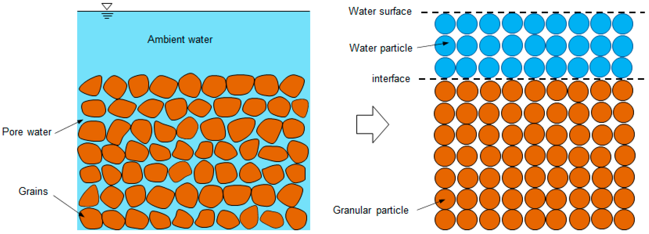
In this SPH model, the approach for multiphase granular flow proposed by Tajnesaie et al. [20] is adopted. As shown in Figure 1, the debris flow is represented by granular-type (in brown color) particles, and the water is represented by fluid-type (in blue color) particles. As the granular flow is quite fast, and the permeability is low, it is assumed in this model that the mass exchange between the ambient and pore water is negligible. Each particle has its own physical and mechanical properties. The fluid-type particles are regarded as Newtonian fluid, and the viscosity is constant. In contrast, the granular-type particles are regarded as Bingham viscous fluid, and the viscosity is variable and determined by the rheological model, as described in Section 2.3.
2.5. Treatment on Water–Soil Interface
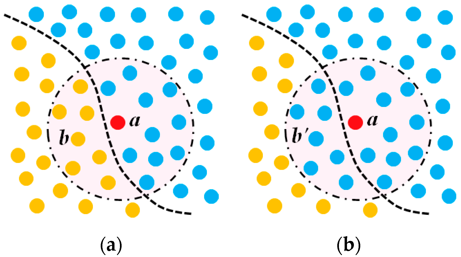
As shown in Figure 2a, density and mass are discontinuous near the water–soil interface, reducing the computational accuracy and stability when solving the governing equations. Therefore, boundary treatments on the water–soil interface should be made when solving the governing equations.
As shown in Figure 2a, a is the central particle (in red) and b represents the neighboring particles of the other phase (in yellow). In this model, particle b is converted into particle b’ (in blue) of the same phase with particle a, as shown in Figure 2b, which occupies the same position, velocity, and volume as the original particle b. Only the position, volume, velocity, and pressure of these neighboring particles are taken into account in particle approximation.
2.6. Boundary Condition
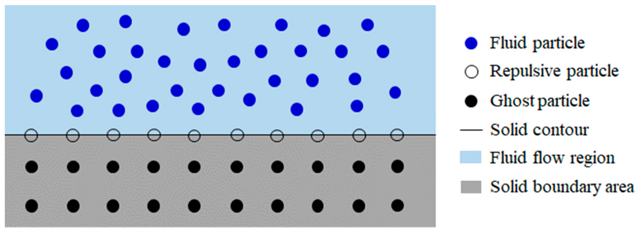
During the submarine debris flow propagation, the fluid particles face resistance from the local seabed. Therefore, to truly simulate the debris flow motion, it is important to accurately calculate the repulsive force from the solid boundary. In the SPH method, repulsive particles are widely used on the boundary contours to exert a force on the fluid particle in the direction of the line connecting both particles, as shown in Figure 3.
The repulsive force, Fij, can be determined by Equation (11) [40]:
where D is a parameter that depends on the highest flow velocity, r0 is the cutoff distance, |rij| is the distance between a fluid particle and a boundary virtual particle, Xij is the difference between the position vectors of a fluid particle and a boundary virtual particle, and n1 and n2 are parameters that are usually equal to 12 and 4, respectively.
3. Model Validation and Application
3.1. Waves Generated by Underwater Rigid Block Sliding
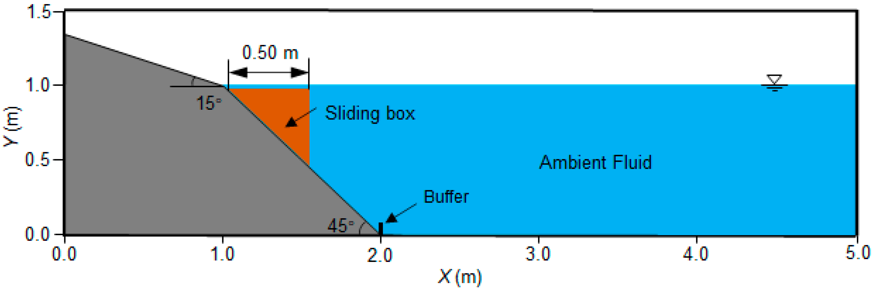
To validate the developed SPH model, an underwater rigid block sliding experiment performed by Heinrich [41] was simulated, and the numerical results were compared with test data. Figure 4 shows the experimental setup. In the experiment, a block slid down a slope of 45° on the horizontal and generated water waves. The shore was simulated by another incline with a 15° slope. Water surface was level with the intersection of these two inclines, and the water depth in the channel was 1 m. The block was triangular in the cross-section with dimensions of 0.5 m × 0.5 m. The density was 2000 kg/m3. During the experiment, the block slid into the water under the effect of gravity, and then stopped when it ran into a small buffer at the channel bottom. As shown in Figure 4, the computational domain was 5.0 m × 1.3 m in the x and y directions. Table 1 lists the calculating parameters used in the SPH simulation.
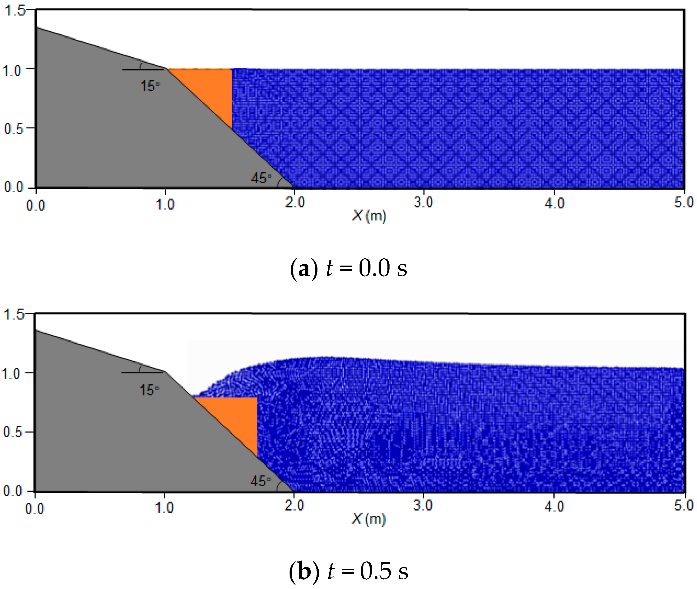
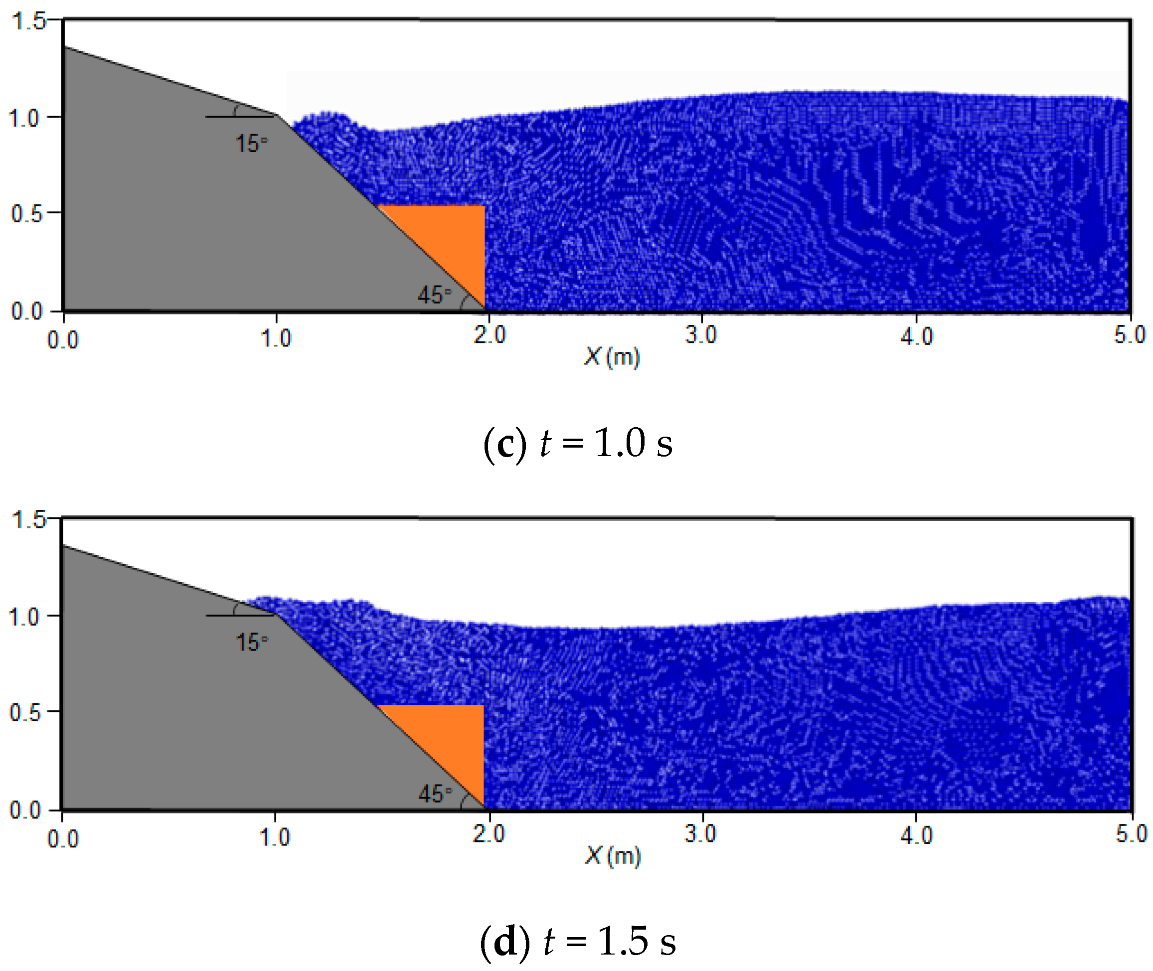
Figure 5 shows the SPH simulated results for the rigid block sliding experiment. When the block slid down, surge waves were generated because the kinetic energy of the sliding block was transferred to the ambient water body. The surge waves propagated out from the near field to the far field because of the height differences of the water surface. Energy conversion finished after the rigid block stopped, and then both the kinetic and potential energy of the water waves started to decay. The positions of the block and the wave profiles at different times were observed.
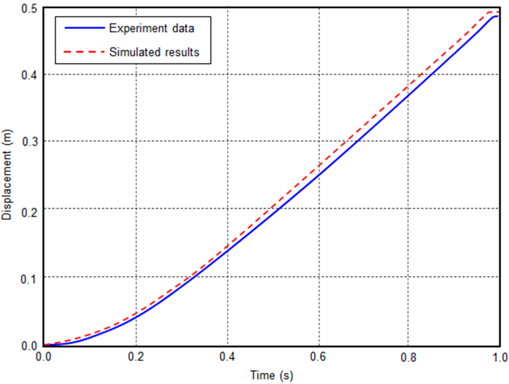
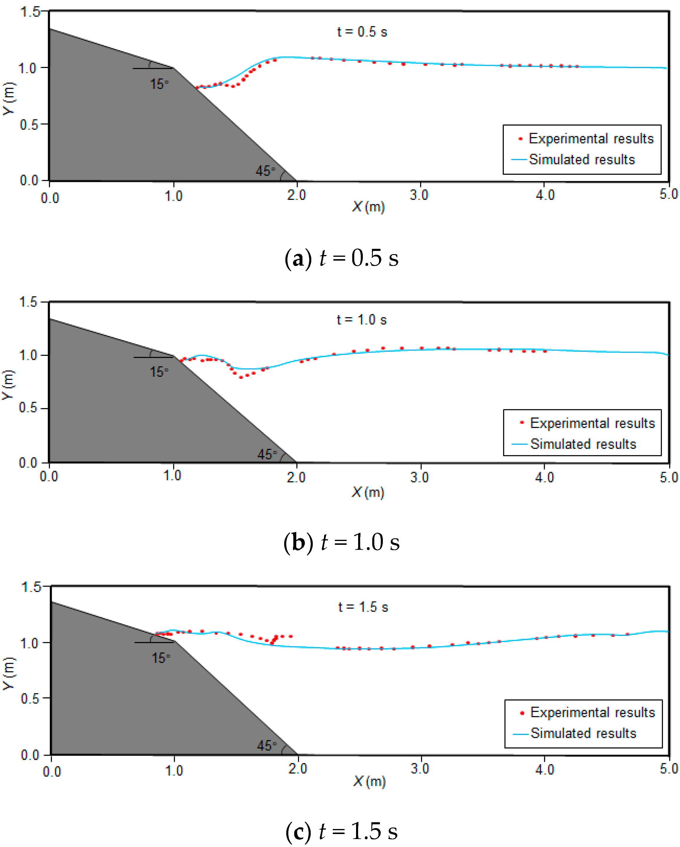
To verify the simulation accuracy of the SPH model, the numerical results were compared with the experimental data from Heinrich [41]. Figure 6 compares the numerical and experimental vertical displacement time history of the rigid block. The numerical results coincided with the experiment data well. After an acceleration phase at the beginning, the rigid block reached a constant velocity of 0.6 m/s. At approximately 1.0 s, the block reached the flume bottom in the SPH model as well as in the experiment. Figure 7 shows the comparison between the simulated and observed wave profiles at different times (t = 0.5 s, t = 1.0 s and t = 1.5 s). Although some discrepancy can be observed, there is close overall agreement between the experimental and numerical wave profiles. The maximum run-up of the wave during the simulation was about 0.10 m, which matches the experimental data well.
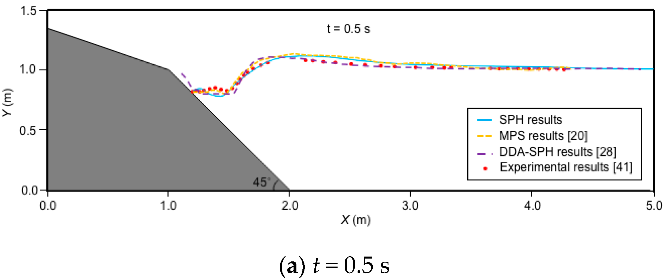
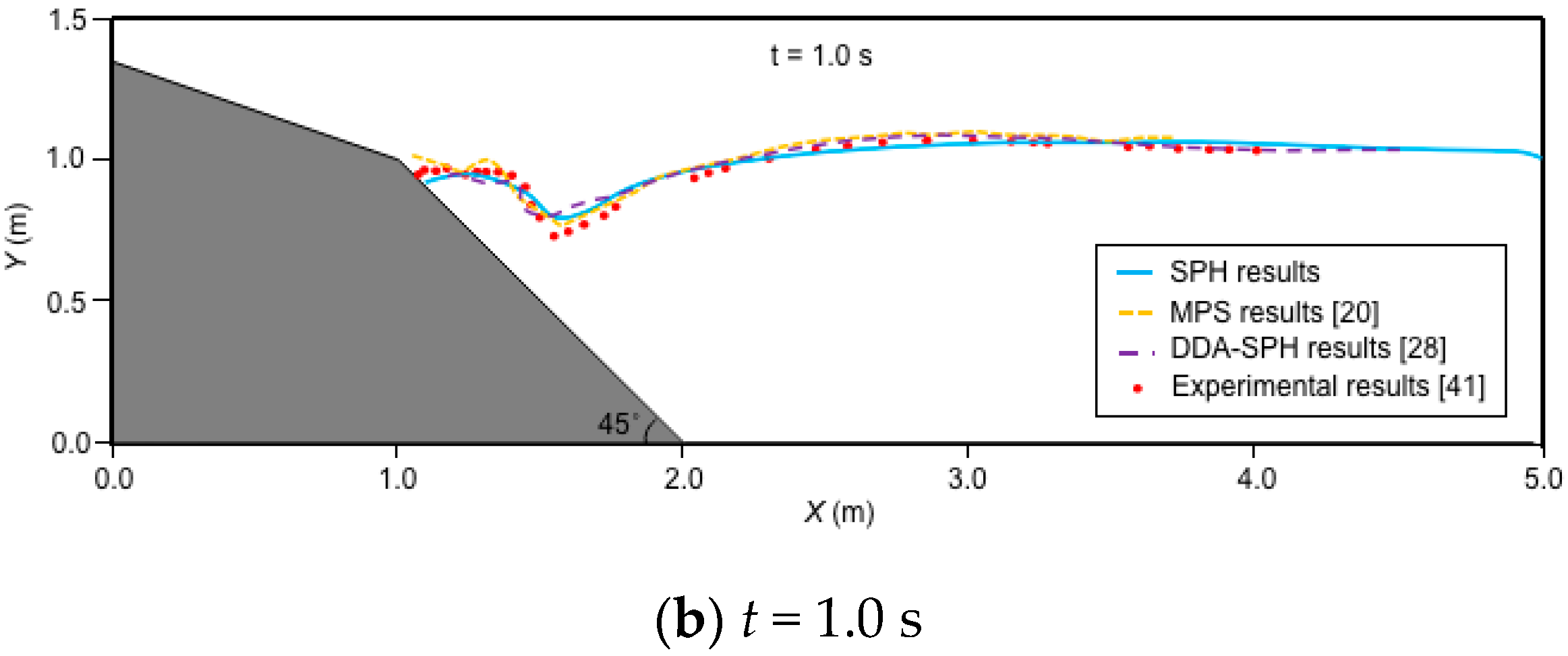
To evaluate the performance of the presented model furtherly, the numerical results are compared with those calculated by Tajnesaie et al. [20] using a MPS model, and Wang et al. [28] using a coupled DDA-SPH model. Figure 8 compares the water profiles calculated based on the above-mentioned numerical models at t = 0.5 s and t = 1.0 s. It shows that all the numerical models produce similar water profiles which are consistent with that observed in the experiments.
To quantitatively compare the results, the Pearson correlation coefficient of the experimental and numerical water profiles in Figure 8 are calculated. In this case, 40 points with an equal horizontal distance on the water profile are selected as the analysis objects. Assuming that the vector X (x1, x2, x3, ……, x40) represents the calculated elevations of these points, and Y (y1, y2, y3, ……, y40) represents the measured ones, the Pearson correlation coefficient of the two vectors can be calculated as:
where and are the average values of the two data sets, respectively.
According to Equation (12), the correlation coefficients between the experimental and numerical results are listed in Table 2. It shows that all the correlation coefficients calculated are close to 1, which means that the numerical results have a strong correlation with the experimental profiles. Therefore, the presented SPH model can successfully simulate such complex flows.
3.2. Waves Generated by the Underwater Sand Flow
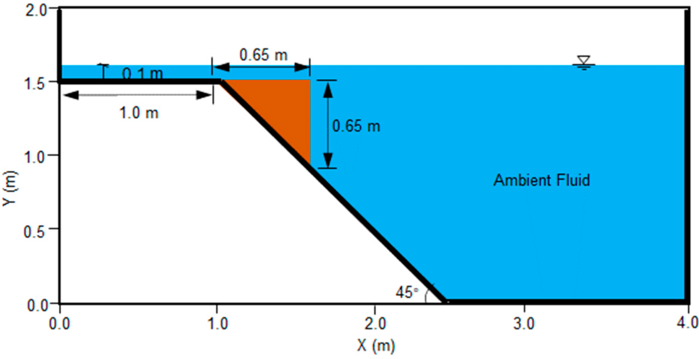
In Section 3.1, the block was assumed to be rigid, which is not consistent with the actual situation of submarine debris flow. The large deformation of the solid phase should be taken into account in the simulation of the submarine debris flow propagation. Therefore, an experiment of the surge waves generated by underwater sand flow, conducted by Rzadkiewicz et al. [42], was simulated. Figure 9 shows the experimental setup. In this experiment, the maximum water depth was 1.6 m. Under the influence of gravity, a mass of sand (0.65 m × 0.65 m in cross section) slid down along a slope of 45°, and generated waves propagated outward.
In the underwater sand flow experiment, the density of the sand was 1950 kg/m3, and the grain diameter ranged from 2 to 7 mm. In the numerical simulation, the sand flow was assumed to be a Bingham fluid. The parameters are listed in Table 3. In the absence of measurements, the viscosity coefficient and yield stress of Bingham model can be determined by trial and error. According to Ataie–Ashtiani and Shobeyri [43], under the conditions of viscosity coefficient ηg = 0.15 Pa·s and Bingham yield stress τy = 750 Pa, the numerical results match the experimental data well. Therefore, the same parameter values were used in this study.
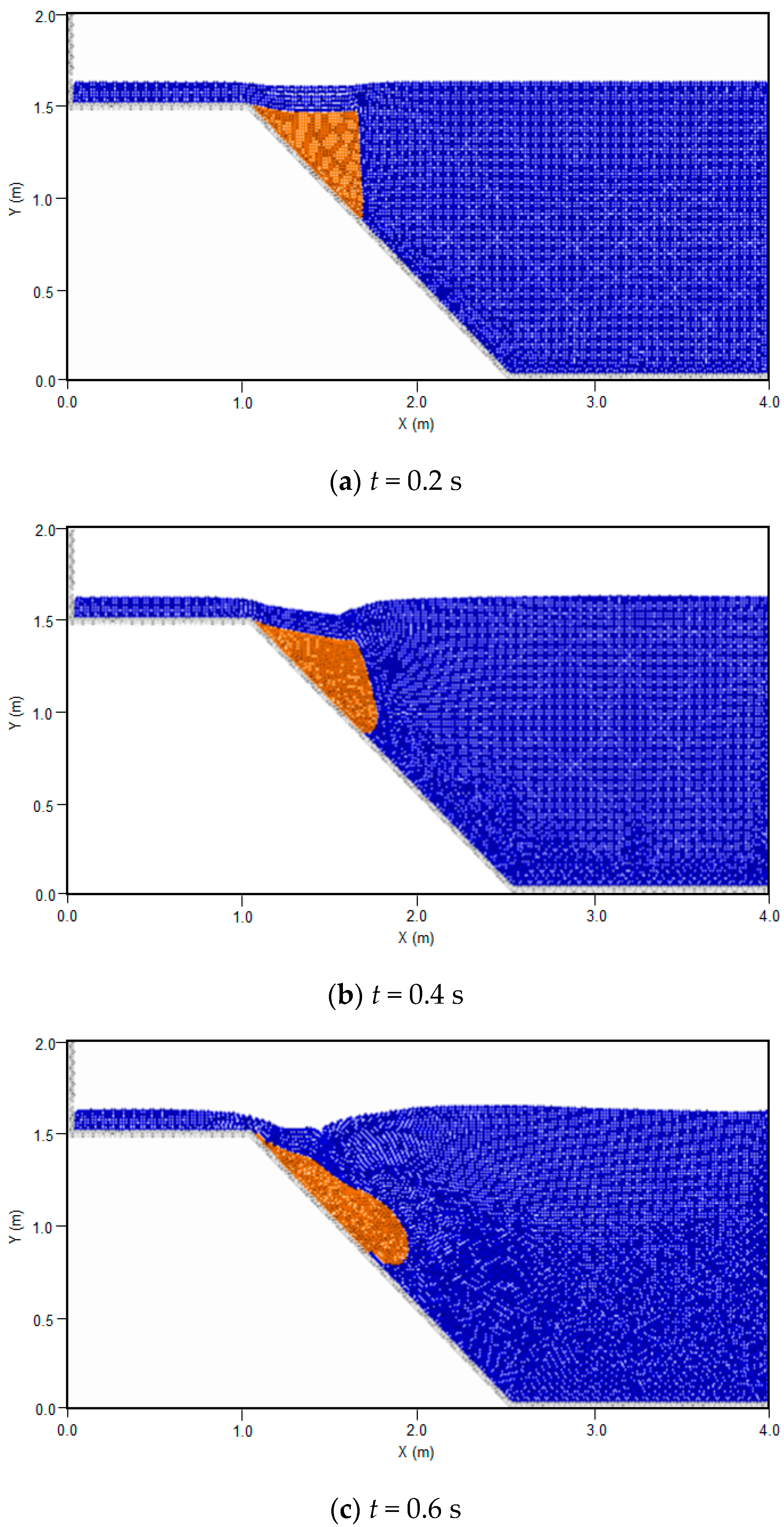
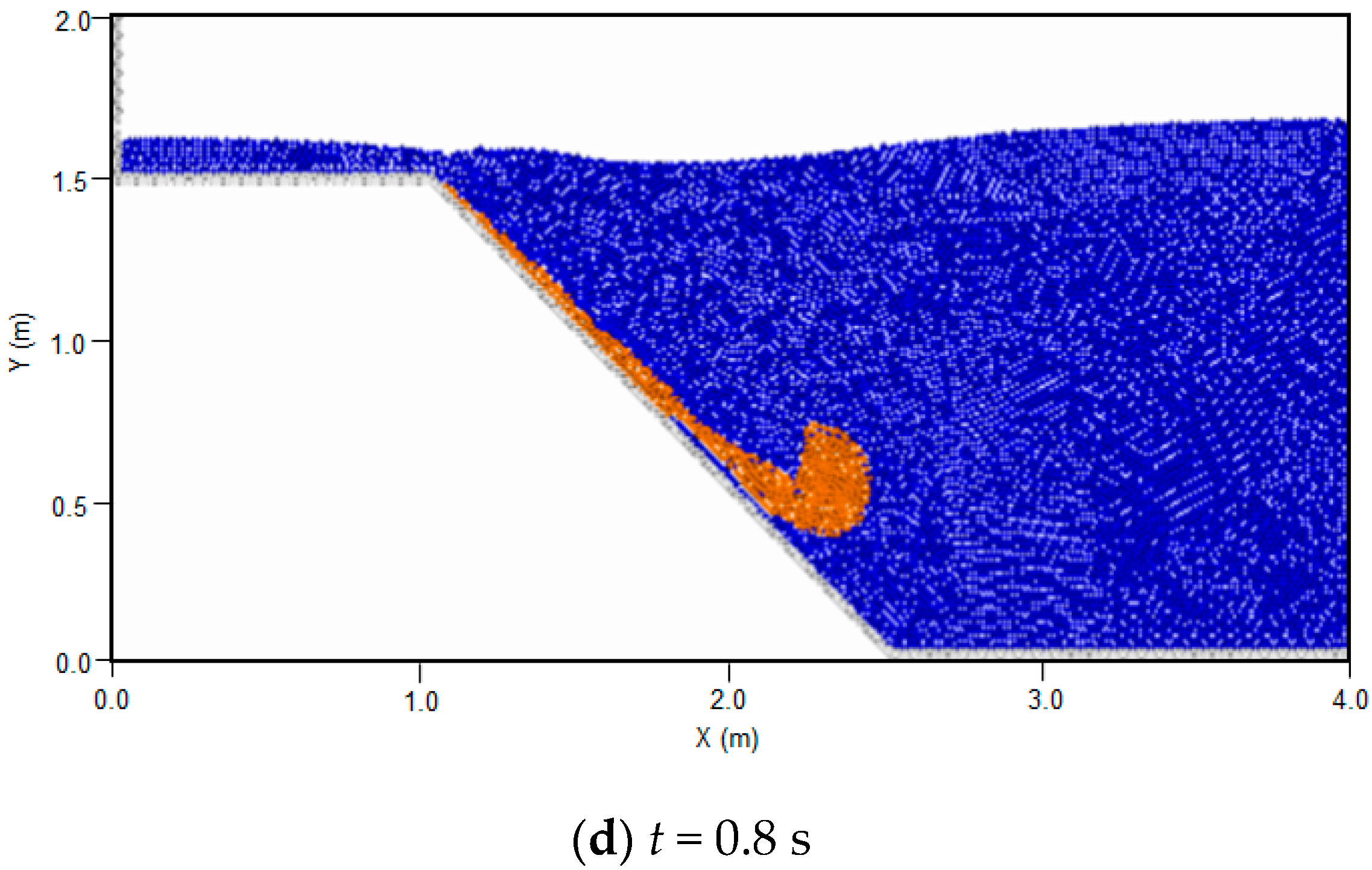
Figure 10 shows the SPH simulated results for the underwater sand flow. Unlike the previous numerical example, the solid phase no longer behaved as a rigid block but deformed significantly when sliding down along the slope. The profiles of water and sand slope at different times are presented. The sand slope keeps its initial shape at the beginning of slide motion, as shown in Figure 9a,b, while at t = 0.8 s, most of the sand particles are concentrated at the flow front, as shown in Figure 9d.
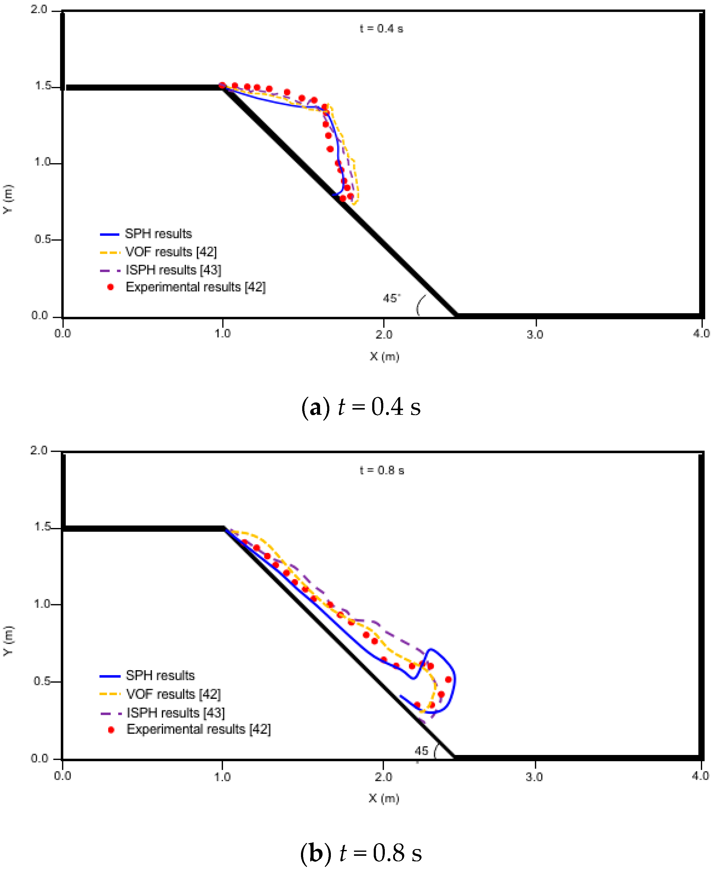
Figure 11 compares the simulated slope configurations with experimental data [42] and those calculated by the VOF model proposed in [42] and the ISPH model proposed in [43]. It shows that the simulated slope configurations are coincident with experimental results. Table 4 lists the Pearson correlation coefficients of the numerical and experimental slope configurations shown in Figure 11. The comparison shows that the SPH model proposed in this study has the equivalent simulation accuracy with the existing numerical models.
4. Conclusions
Submarine debris flow-generated water waves are natural phenomena that occur under certain conditions and can result in damage of infrastructure and loss of life in coastal areas. In this study, an SPH model with a multiphase granular flow algorithm is presented for numerical simulation of surge waves generated by submarine debris flows. The Bingham fluid model and Newton fluid model are used to describe the motion behavior of submarine debris flow and ambient water, respectively. A simple treatment is proposed to ensure the continuity of the density and pressure near the interface of these two fluids and to avoid numerical instability.
This model was first used to simulate an experiment of underwater rigid block sliding. The simulated wave profiles were compared with the observed results to verify the stability and accuracy of the SPH model.
Then, this model was applied to simulate submarine debris flow. Surged waves generated by the underwater sand flow were computed and compared with the tested results. The good agreement between the numerical and tested results proves that the proposed SPH model is suitable to simulate such complex flows.
In fact, submarine debris flows move across 3D submarine topography and may change direction and split or join in response to the complex topography. Therefore, the 2D model presented in this study cannot truly reproduce the complex dynamic process, and a 3D model with parallel computing techniques is necessary to improve the calculation accuracy and efficiency.
Author Contributions
Conceptualization, Z.D. and S.Q.; methodology, Z.D. and J.X.; writing—original draft preparation, Z.D. and J.X.; writing—review and editing, S.Q. and S.C.; visualization, J.X. and S.C.; supervision, S.Q.; funding acquisition, Z.D. All authors have read and agreed to the published version of the manuscript.
Funding
This research was funded by the National Natural Science Foundation of China (grant No. 42102318) and the Program for Professor of Special Appointment (Eastern Scholar) at Shanghai Institutions of Higher Learning.
Institutional Review Board Statement
Not applicable.
Informed Consent Statement
Not applicable.
Data Availability Statement
The data presented in this study are available on request from the corresponding author.
Acknowledgments
The authors are grateful for the support from the Department of Civil Engineering, Shanghai University.
Conflicts of Interest
The authors declare no conflict of interest.
References
- Nian, T.K.; Guo, X.S.; Zheng, D.F.; Xiu, Z.X.; Jiang, Z.B. Susceptibility assessment of regional submarine landslides triggered by seismic actions. Appl. Ocean Res. 2019, 93, 101964. [Google Scholar] [CrossRef]
- Gonzalez-Vida, J.M.; Macias, J.; Castro, M.J.; Sanchez-Linares, C.; de la Asuncion, M.; Ortega-Acosta, S.; Arcas, D. The Lituya Bay landslide-generated mega-tsunami—numerical simulation and sensitivity analysis. Nat. Hazards Earth Syst. Sci. 2019, 19, 369–388. [Google Scholar] [CrossRef] [Green Version]
- Dan, G.; Sultan, N.; Savoye, B. The 1979 Nice harbour catastrophe revisited: Trigger mechanism inferred from geotechnical measurements and numerical modelling. Mar. Geol. 2007, 245, 40–64. [Google Scholar] [CrossRef] [Green Version]
- Rabinovich, A.B.; Thomson, R.E.; Kulikov, E.A.; Bornhold, B.D.; Fine, I.V. The landslide-generated tsunami of November 3, 1994 in Skagway Harbor, Alaska: A case study. Geophys. Res. Lett. 1999, 26, 3009–3012. [Google Scholar] [CrossRef]
- Sabeti, R.; Heidarzadeh, M. Semi-empirical predictive equations for the initial amplitude of submarine landslide-generated waves: Applications to 1994 Skagway and 1998 Papua New Guinea tsunamis. Nat. Hazards 2020, 103, 1591–1611. [Google Scholar] [CrossRef]
- Heidarzadeh, M.; Satake, K. Source properties of the 17 July 1998 Papua New Guinea tsunami based on tide gauge records. Geophys. J. Int. 2015, 202, 361–369. [Google Scholar] [CrossRef] [Green Version]
- Hébert, H.; Burg, P.E.; Binet, R.; Lavigne, F.; Allgeyer, S.; Schindelé, F. The 2006 July 17 Java (Indonesia) tsunami from satellite imagery and numerical modelling: A single or complex source? Geophys. J. Int. 2012, 191, 1255–1271. [Google Scholar] [CrossRef] [Green Version]
- Poupardin, A.; Calais, E.; Heinrich, P.; Hebert, H.; Rodriguez, M.; Leroy, S.; Aochi, H.; Douilly, R. Deep submarine landslide contribution to the 2010 Haiti earthquake tsunami. Nat. Hazards Earth Syst. Sci. 2020, 20, 2055–2065. [Google Scholar] [CrossRef]
- Muhari, A.; Imamura, F.; Arikawa, T.; Hakim, A.; Afriyanto, B. Solving the Puzzle of the September 2018 Palu, Indonesia, Tsunami Mystery: Clues from the Tsunami Waveform and the Initial Field Survey Data. J. Disaster Res. 2018, 13, sc20181108. [Google Scholar] [CrossRef]
- Arikawa, T.; Muhari, A.; Okumura, Y.; Dohi, Y.; Afriyanto, B.; Sujatmiko, K.A.; Imamura, F. Coastal subsidence induced several tsunamis during the 2018 Sulawesi earthquake. J. Disaster Res. 2018, 13, sc20181204. [Google Scholar] [CrossRef]
- Sassa, S.; Takagawa, T. Liquefied gravity flow-induced tsunami: First evidence and comparison from the 2018 Indonesia Sulawesi earthquake and tsunami disasters. Landslides 2019, 16, 195–200. [Google Scholar] [CrossRef] [Green Version]
- Mohammed, F.; Fritz, H.M. Physical modeling of tsunamis generated by three-dimensional deformable granular landslides. J. Geophys. Res. Ocean 2012, 117, C11015. [Google Scholar] [CrossRef] [Green Version]
- McFall, B.C.; Fritz, H.M. Physical modelling of tsunamis generated by three-dimensional deformable granular landslides on planar and conical island slopes. Proc. R. Soci. A Math. Phys. Eng. Sci. 2016, 472, 20160052. [Google Scholar] [CrossRef] [PubMed] [Green Version]
- Wang, Y.; Liu, J.Z.X.; Li, D.Y.; Yan, S.J. Optimization model for maximum tsunami amplitude generated by riverfront landslides based on laboratory investigations. Ocean Eng. 2017, 142, 433–440. [Google Scholar] [CrossRef]
- Miller, G.S.; Take, W.A.; Mulligan, R.P.; McDougall, S. Tsunamis generated by long and thin granular landslides in a large flume. J. Geophys. Res. Ocean 2017, 122, 653–668. [Google Scholar] [CrossRef]
- Meng, Z.Z. Experimental study on impulse waves generated by a viscoplastic material at laboratory scale. Landslides 2018, 15, 1173–1182. [Google Scholar] [CrossRef]
- Takabatake, T.; Mall, M.; Han, D.C.; Inagaki, N.; Kisizaki, D.; Esteban, M.; Shibayama, T. Physical modeling of tsunamis generated by subaerial, partially submerged, and submarine landslides. Coast. Eng. J. 2020, 4, 582–601. [Google Scholar] [CrossRef]
- Lynett, P.; Liu, P.L.F. A numerical study of submarine-landslide-generated waves and run-up. Proc. R. Soc. A Math. Phys. Eng. Sci. 2002, 458, 2885–2910. [Google Scholar] [CrossRef]
- Yavari-Ramshe, S.; Ataie-Ashtiani, B. Numerical modeling of subaerial and sub- marine landslide-generated tsunami waves-recent advances and future challenges. Landslides 2016, 13, 1325–1368. [Google Scholar] [CrossRef]
- Tajnesaie, M.; Shakibaeinia, A.; Hosseini, K. Meshfree particle numerical modelling of sub-aerial and submerged landslides. Comput. Fluids 2018, 172, 109–121. [Google Scholar] [CrossRef]
- Sun, J.K.; Wang, Y.; Huang, C.; Wang, W.H.; Wang, H.B.; Zhao, E.J. Numerical investigation on generation and propagation characteristics of offshore tsunami wave under landslide. Appl. Sci. 2020, 10, 5579. [Google Scholar] [CrossRef]
- Rupali; Kumar, P.; Rajni. Spectral wave modeling of tsunami waves in Pohang New Harbor (South Korea) and Paradip Port (India). Ocean Dyn. 2020, 70, 1515–1530. [Google Scholar] [CrossRef]
- Baba, T.; Gon, Y.; Imai, K.; Yamashita, K.; Matsuno, T.; Hayashi, M.; Ichihara, H. Modeling of a dispersive tsunami caused by a submarine landslide based on detailed bathymetry of the continental slope in the Nankai trough, southwest Japan. Tectonophysics 2019, 768, 228182. [Google Scholar] [CrossRef]
- Yao, Y.; He, T.; Deng, Z.; Chen, L.; Guo, H. Large eddy simulation modeling of tsunami-like solitary wave processes over fringing reefs. Nat. Hazards Earth Syst. Sci. 2019, 19, 1281–1295. [Google Scholar] [CrossRef] [Green Version]
- Zhao, E.; Sun, J.; Tang, Y.; Mu, L.; Jiang, H. Numerical investigation of tsunami wave impacts on different coastal bridge decks using immersed boundary method. Ocean Eng. 2020, 201, 107132. [Google Scholar] [CrossRef]
- Lucy, L.B. A numerical approach to the testing of the fission hypothesis. Astrophys. J. 1977, 82, 1013–1024. [Google Scholar] [CrossRef]
- Iryanto, I. SPH simulation of surge waves generated by aerial and submarine landslides. J. Phys. Conf. Ser. 2019, 1245, 012062. [Google Scholar] [CrossRef] [Green Version]
- Wang, W.; Chen, G.Q.; Zhang, H.; Zhou, S.H.; Liu, S.G.; Wu, Y.Q.; Fan, F.S. Analysis of landslide-generated impulsive waves using a coupled DDA-SPH method. Eng. Anal. Bound. Elem. 2016, 64, 267–277. [Google Scholar] [CrossRef]
- Gingold, R.A.; Monaghan, J.J. Smoothed particle hydrodynamics: Theory and application to non-spherial stars. Mon. Not. R. Astron. Soc. 1977, 181, 375–389. [Google Scholar] [CrossRef]
- Dai, Z.L.; Huang, Y.; Cheng, H.L.; Xu, Q. SPH model for fluid–structure interaction and its application to debris flow impact estimation. Landslides 2017, 14, 917–928. [Google Scholar] [CrossRef]
- Dai, Z.L.; Huang, Y.; Xu, Q. A hydraulic soil erosion model based on a weakly compressible smoothed particle hydrodynamics method. Bull. Eng. Geol. Environ. 2019, 78, 5853–5864. [Google Scholar] [CrossRef]
- Jamalabadi, M.Y.A. Frequency analysis and control of sloshing coupled by elastic walls and foundation with smoothed particle hydrodynamics method. J. Sound Vib. 2020, 476, 115310. [Google Scholar] [CrossRef]
- Price, D.J.; Laibe, G. A solution to the overdamping problem when simulating dust-gas mixtures with smoothed particle hydrodynamics. Mon. Not. R. Astron. Soc. 2020, 495, 3929–3934. [Google Scholar] [CrossRef]
- Ma, C.; Iijima, K.; Oka, M. Nonlinear waves in a floating thin elastic plate, predicted by a coupled SPH and FEM simulation and by an analytical solution. Ocean Eng. 2020, 204, 107243. [Google Scholar] [CrossRef]
- Liu, M.B.; Liu, G.R. Smoothed particle hydrodynamics (SPH): An overview and recent developments. Arch. Comput. Methods Eng. 2010, 17, 25–76. [Google Scholar] [CrossRef] [Green Version]
- Shakibaeinia, A.; Jin, Y.C. MPS mesh-free particle method for multiphase flows. Comput. Methods Appl. Mech. Eng. 2012, 229, 13–26. [Google Scholar] [CrossRef]
- Monaghan, J.J.; Cas, R.F.; Kos, A.; Hallworth, M. Gravity currents descending a ramp in a stratified tank. J. Fluid Mech. 1999, 379, 39–70. [Google Scholar] [CrossRef]
- Zheng, B.; Chen, Z. A multiphase smoothed particle hydrodynamics model with lower numerical diffusion. J. Comput. Phys. 2019, 382, 177–201. [Google Scholar] [CrossRef]
- Zhang, W.J.; Ji, J.; Gao, Y.F. SPH-based analysis of the post-failure flow behavior for soft and hard interbedded earth slope. Eng. Geol. 2020, 267, 105446. [Google Scholar] [CrossRef]
- Monaghan, J.J. Simulating free surface flows with SPH. J. Comput. Phys. 1994, 110, 399–406. [Google Scholar] [CrossRef]
- Heinrich, P. Nonlinear water waves generated by submarine and aerial landslides. J. Waterw. Port Coast. Ocean Eng. 1992, 118, 249–266. [Google Scholar] [CrossRef]
- Rzadkiewicz, S.A.; Mariotti, C.; Heinrich, P. Numerical simulation of submarine landslides and their hydraulic effects. J. Waterw. Port Coast. Ocean Eng. 1997, 123, 149–157. [Google Scholar] [CrossRef]
- Ataie-Ashtiani, B.; Shobeyri, G. Numerical simulation of landslide impulsive waves by incompressible smoothed particle hydrodynamics. Int. J. Numer. Methods Fluids 2008, 56, 209–232. [Google Scholar] [CrossRef]
Figure 1.
Particle representation of multiphase granular continuum.

Figure 2.
Treatment on the interface of different fluids: (a) original particles; (b) converted particles.
Figure 2.
Treatment on the interface of different fluids: (a) original particles; (b) converted particles.

Figure 3.
Schematic illustration of the solid boundary treatment.

Figure 4.
Experimental setup of an underwater rigid block sliding along an inclined plane.

Figure 5.
SPH simulated results for the rigid block sliding experiment: (a) t = 0.0 s; (b) t = 0.5 s; (c) t = 1.0 s; (d) t = 1.5 s.
Figure 5.
SPH simulated results for the rigid block sliding experiment: (a) t = 0.0 s; (b) t = 0.5 s; (c) t = 1.0 s; (d) t = 1.5 s.


Figure 6.
Comparison between the numerical and experimental vertical displacement time history of the rigid block.
Figure 6.
Comparison between the numerical and experimental vertical displacement time history of the rigid block.

Figure 7.
Comparison between the simulated and observed wave profiles at different times: (a) t = 0.5 s; (b) t = 1.0 s; (c) t = 1.5 s.
Figure 7.
Comparison between the simulated and observed wave profiles at different times: (a) t = 0.5 s; (b) t = 1.0 s; (c) t = 1.5 s.

Figure 8.
Comparison of the experimental and numerical (from the models of current study and other numerical studies) water profiles at different times: (a) t = 0.5 s; (b) t = 1.0 s.
Figure 8.
Comparison of the experimental and numerical (from the models of current study and other numerical studies) water profiles at different times: (a) t = 0.5 s; (b) t = 1.0 s.


Figure 9.
Experimental setup of the underwater sand flow.

Figure 10.
SPH simulated results for the underwater sand flow: (a) t = 0.2 s; (b) t = 0.4 s; (c) t = 0.6 s; (d) t = 0.8 s.
Figure 10.
SPH simulated results for the underwater sand flow: (a) t = 0.2 s; (b) t = 0.4 s; (c) t = 0.6 s; (d) t = 0.8 s.


Figure 11.
Comparison of the experimental and numerical (from the models of current study and other numerical studies) slope configurations at different times: (a) t = 0.4 s; (b) t = 0.8 s.
Figure 11.
Comparison of the experimental and numerical (from the models of current study and other numerical studies) slope configurations at different times: (a) t = 0.4 s; (b) t = 0.8 s.


Table 1.
Parameters used in the SPH simulation of the rigid block sliding experiment.
| Rigid block density | ρs (kg/m3) | 2000 |
| Water density | ρw (kg/m3) | 1000 |
| Water viscosity coefficient | η (Pa·s) | 1.7 × 10⁻³ |
| Acceleration of gravity | g (m/s2) | 9.8 |
Table 2.
Correlation coefficients between the experimental and numerical results on the water profiles.
Table 2.
Correlation coefficients between the experimental and numerical results on the water profiles.
| Case | Current Study | Tajnesaie et al. [20] | Wang et al. [28] |
|---|---|---|---|
| t = 0.5 | 0.9336 | 0.9389 | 0.9297 |
| t = 1.0 | 0.9132 | 0.9206 | 0.9040 |
Table 3.
Parameters used in the SPH simulation of underwater sand flow.
| Density of sand | ρs (kg/m3) | 1950 |
| Viscosity coefficient of sand flow | ηg (Pa·s) | 0.15 |
| Bingham yield stress of sand flow | τy (Pa) | 750 |
| Density of water | ρw (kg/m3) | 1000 |
| Viscosity coefficient of water | ηw (Pa·s) | 1.7 × 10⁻³ |
| Acceleration of gravity | g (m/s2) | 9.8 |
Table 4.
Correlation coefficients between the experimental and numerical results on the water profiles.
Publisher’s Note: MDPI stays neutral with regard to jurisdictional claims in published maps and institutional affiliations. |
© 2021 by the authors. Licensee MDPI, Basel, Switzerland. This article is an open access article distributed under the terms and conditions of the Creative Commons Attribution (CC BY) license (https://creativecommons.org/licenses/by/4.0/).
Share and Cite
MDPI and ACS Style
Dai, Z.; Xie, J.; Qin, S.; Chen, S. Numerical Investigation of Surge Waves Generated by Submarine Debris Flows. Water 2021, 13, 2276. https://doi.org/10.3390/w13162276
AMA Style
Dai Z, Xie J, Qin S, Chen S. Numerical Investigation of Surge Waves Generated by Submarine Debris Flows. Water. 2021; 13(16):2276. https://doi.org/10.3390/w13162276
Chicago/Turabian StyleDai, Zili, Jinwei Xie, Shiwei Qin, and Shuyang Chen. 2021. "Numerical Investigation of Surge Waves Generated by Submarine Debris Flows" Water 13, no. 16: 2276. https://doi.org/10.3390/w13162276
Note that from the first issue of 2016, this journal uses article numbers instead of page numbers. See further details here.