
Can Managed Aquifer Recharge Overcome Multiple Droughts?


1
Department of Civil and Environmental Engineering, Washington State University, Pullman, WA 99164-2910, USA
2
Earth System Science Interdisciplinary Center, University of Maryland, College Park, MD 20740-3823, USA
3
School of the Environment, Washington State University, Pullman, WA 99164-2812, USA
*
Author to whom correspondence should be addressed.
Water 2021, 13(16), 2278; https://doi.org/10.3390/w13162278
Submission received: 22 July 2021
/
Revised: 13 August 2021
/
Accepted: 14 August 2021
/
Published: 20 August 2021
(This article belongs to the Special Issue Water Resources Systems in a Changing World: Planning and Adaptation)
Abstract
:Frequent droughts, seasonal precipitation, and growing agricultural water demand in the Yakima River Basin (YRB), located in Washington State, increase the challenges of optimizing water provision for agricultural producers. Increasing water storage through managed aquifer recharge (MAR) can potentially relief water stress from single and multi-year droughts. In this study, we developed an aggregated water resources management tool using a System Dynamics (SD) framework for the YRB and evaluated the MAR implementation strategy and the effectiveness of MAR in alleviating drought impacts on irrigation reliability. The SD model allocates available water resources to meet instream target flows, hydropower demands, and irrigation demand, based on system operation rules, irrigation scheduling, water rights, and MAR adoption. Our findings suggest that the adopted infiltration area for MAR is one of the main factors that determines the amount of water withdrawn and infiltrated to the groundwater system. The implementation time frame is also critical in accumulating MAR entitlements for single-year and multi-year droughts mitigation. In addition, adoption behaviors drive a positive feedback that MAR effectiveness on drought mitigation will encourage more MAR adoptions in the long run. MAR serves as a promising option for water storage management and a long-term strategy for MAR implementation can improve system resilience to unexpected droughts.
1. Introduction
Satisfying water resource demands across food, energy, and water (FEW) systems is a growing concern due to rapid socio-economic development and population growth [1,2,3,4]. On the other hand, water supply is vulnerable due to climate uncertainty and variability at different temporal and spatial scales. The increasing frequency of extreme climatic events [5,6], such as floods and droughts, and the shifting seasonality [7], bring unexpected problems to sectors like agriculture whose production depends heavily on the quantity and timing of water supply [8]. Seasonal shifts in the hydrologic cycle and reduced dry-season water availability [9] generate extra challenges to water allocation in snow-dominated regions like the Pacific Northwest (USA). Facing increased water scarcity, undesirable trade-offs must often be made when inadequate water availability causes failure to satisfy demand due to competing needs by domestic and industrial, irrigation, fire preparedness, and natural systems [10,11,12]. Integrated water resources management is needed to allocate water strategically in space and time to achieve synergies in the long term [13].
Demand and supply management in FEW systems coping with water scarcity recently has considered increased storage capacity options [14,15], such as increased surface reservoir capacity and managed aquifer recharge. Increasing storage capacities in supply management of reservoirs, however, occasionally fails to satisfy all water demands during drought due to limited storage space and conflicts among multiple objectives [16], such as environmental impacts [17] and cost–benefit ratios [18]. Managed aquifer recharge (MAR) intentionally stores extra water in the subsurface, rather than releasing it downstream, and expands adaptive capacity, sustains groundwater levels [19], and can recover streamflow [20,21,22].
Various techniques may be used to either recharge water (e.g., infiltration basin and well injection) or intercept water (e.g., runoff harvesting), depending on location conditions [23]. With regard to the cost and simplicity, there is increasing interest in spreading water on agricultural land for infiltration with water delivered by existing canals during winter or fallow periods [24]. Hydrogeological conditions, site-specific objectives, and sociological norms are the main factors for MAR design and implementation [20]. Specifically for Washington state with legal procedures to regulate MAR [25], there is yet to be operational MAR at the level of irrigation districts or cities. A framework is needed that can evaluate MAR scenarios in anticipation of future climate variability. Identifying MAR strategies based on interconnections, drivers, and metrics within the context of the FEW nexus [26] can help minimize water management failures stemming from limited understanding of system behavior [27,28,29].
A promising framework for the evaluation of MAR is system dynamics (SD) modeling [21,30,31,32] because of its ability to encompass interconnectivity of system components and how systems change over time in response to perturbations in climate, human behavior, and adaptations. SD modeling uses “stocks and flows” to represent non-linear dynamics of complex systems and enhances our understandings of dynamic behaviors by capturing feedback processes, time delays, and factors of dynamic complexity [33]. SD modeling has been applied to a variety of disciplines including policy-making [34], resource management [31,35], economic systems [36], socio-ecological systems [37], and in business [38] while incorporating socioeconomic and environmental impacts [39,40,41,42,43]. The transparent structure and incorporation-oriented features of SD modeling [40] make it a great tool for solving MAR related questions. Whether it is proposing solutions through optimizing resources [44] or conducting scenario discovery in collaborations with stakeholders [35], SD modeling has been proven to be a useful tool to assist with decision-making.
A few examples of SD modeling for evaluation of MAR have emerged in the literature. Ryu et al. [32] used SD modeling to compare five alternative MAR management plans to identify the impact of hydroclimate variability on surface-water and groundwater interactions in the Eastern Snake Plain Aquifer. Niazi et al. [45] developed a spatial SD model to evaluate the hydrologic and economic outcomes from different aquifer storage and recovery options to assist decision-making. Gibson and Campana [21] identified groundwater recharge zones in the Yakima River Basin and compared surface water capture for groundwater storage for two drought years and a wet year using SD framework. These efforts provided site-specific recommendations that can promote collaborative groundwater expansion [35].
Improved FEW system management requires integration of physical and ecological system dynamics and human decision-making, preferably using mixed-method approaches [4] combining quantitative and qualitative methods. While physically-based modeling for earth systems is well established, incorporating human dimensions such as adoption of new innovations is a strength of SD modeling [32]. Human behavior within socioeconomic systems drives demand and supply cycles in the short-term and in the long-term. As a result, solutions are often counterintuitive for a complex system due to feedback and delay [46]. Integrated approaches, therefore, are particularly useful in assessing potential consequences under future scenarios for complex system like the FEW [47].
In this paper, the objective was to evaluate the effectiveness of MAR as a water storage management practice under different drought conditions in a FEW system. We developed an integrated SD model as an adaptive water resource management tool that focuses on causalities, delays, and feedbacks in the FEW context. An interdisciplinary conceptual map was first created to define the FEW nexus for this work. Second, we selected the Yakima River Basin (YRB) as a case study because this region heavily depends on agricultural production, while water resources have been the most severe issue for stakeholders. Based on available data from various resources [48,49], we developed the SD model combining the conceptual map and YRB characteristics. Third, MAR scenarios, including adoption-diffusion based on norms, advertising, and popularity, were assessed for their effectiveness in improving water scarcity during drought events. Lastly, drivers and feedbacks centered on MAR were evaluated to inform the long-term strategies in MAR design.
2. Study Area
2.1. Yakima River Basin Description
The Yakima River Basin (YRB) is located in south-central Washington with elevations ranging from 2494 m in the Cascades to 104 m in the Yakima River delta. The YRB is bounded by headwaters on the upper eastern slope of the Cascade Range and an arid lower basin with approximately 2500 mm and 150 mm annual precipitation on average, respectively. About 75% of the precipitation occurs during October to March, and the majority falls as snow during winter and early spring. The highly uneven distribution of precipitation spatially and temporally results in annual streamflow peaks that vary from approximately 340 m3/s around May to 30 m3/s around October. The hydrogeologic units consist of low transmitting layers at the upper YRB and permeable alluvial aquifers at the lower YRB [50]. Precipitation-induced groundwater recharge at the lower YRB is limited during the summer, and its seasonal patterns are closely related to irrigation diversion and pumping activities [51].
Five reservoirs (Keechelus, Kachess, Cle Elum, Tieton/Rimrock Dam, Bumping Lake) are located along the tributaries of the Yakima and Naches rivers before they join above Parker station, which is the control point for specific water management decisions (Figure 1). These reservoirs provide water storage for irrigation, flood control, and instream flow requirements. Incoming streamflow is stored in the reservoirs while meeting downstream environmental flow requirements during the winter until late June when storage releases begin. Two hydropower plants, Roza and Chandler, operated by U.S. Bureau of Reclamation (USBR), are primarily used to supply energy for pumping and power station service. Power subordinations for these two power plants occur when there is reduced power generation to improve the fishery flow and maintain an 11.3 m3/s (400 cfs) target flow in the Yakima River below the Roza dam [52]. Part of the water withdrawal from the Yakima River above Parker station to the Roza irrigation canal is delivered to the Roza power plant for hydroelectricity generation, where the used water will return to the Yakima River above Parker station. Chandler hydropower withdrawal is at the Prosser Diversion Dam, which is downstream of Parker station [53].
Irrigation districts encompass over 2000 km2 in the lower semiarid to arid part of the YRB including Kittitas, Tieton, Wapato, Roza, Sunnyside, and Kennewick. More than 50% of irrigated land are cropped with fruit trees and alfalfa [54]. Irrigation seasons are typically from mid-March to mid-October, when about 45% of water diverted for irrigation eventually returns back to the river or recharges groundwater over a span of time [55]. Irrigation water demand takes up more than 60% of annual unregulated flows (4.2 × 10⁹ m3, on average) in the YRB [52]. Surface water rights (non-proratable and proratable) constrain the amount of surface water delivered to water users. When prorationing happens during drought years, junior (i.e., proratable) water right holders will receive the same percentage of their entitlements. Groundwater rights in the YRB consist of 2575 certificates, 299 permits, and 16,600 claims for withdrawal of 0.38 × 10⁹ m3 of water [56], 80% of which are used for irrigation of 525 km2.
2.2. Historical Droughts
Since 1979, ten droughts have caused prorationing in the YRB, resulting in millions of dollars of economic losses in agriculture. Hydrological drought, a term for negative anomalies in a water system above and below ground, is driven by abnormal precipitation and temperature [57]. In snow-dominated regions like the YRB, early or late snowmelt and low snowfall play an important role in the occurrence of droughts during the growing season. We applied threshold levels [58] to identify the severity and duration of droughts in water resources management. Threshold levels are based on the flow duration curve over a 30-day moving window [59]. The daily threshold is the 80th percentile on that curve.
Volume deficits between streamflow and the threshold level were used to understand drought characteristics for scenario analysis in this study. This resulted in the selection of six drought years (1992, 1993, 1994, 2001, 2005, and 2015) (Figure 2). The period of 1992–1994 is a multi-year drought on record [52] with the characteristic that the water system had not fully recovered from the previous drought before the next drought started. The droughts of 1992 and 1994 were more severe than the drought of 1993 according to proration rate data, and both these droughts started in mid-May with long lasting water deficit conditions. During the 1992 flood season, peak reservoir storage was more than 90% of its capacity and reached the minimum storage level [60] due to insufficient streamflow, which was caused by early snowmelt and a warm winter.
Single year droughts in 2001, 2005, and 2015 have distinguishing features (Figure 2). For the 2001 and 2005 droughts, the winter precipitation was below average and there was an abnormally low snowpack due to high temperatures during a few critical winter precipitation events. This resulted in low streamflow during spring and summer [61] when reservoirs only filled up to 64% and 82% of maximum capacity, respectively, compared to the average peak storage of 95% according to historical reservoir storage data [62]. The first of April snow water equivalent for 2015 was similarly low as 2001 and 2005 but due to different factors [63]. The average winter temperature and average winter precipitation for 2015 were both greater than in 2001 and 2005. In addition, the 2015 drought simultaneously experienced above normal winter runoff, due to high spring temperatures that caused early melting of the snowpack, and warm conditions that persisted into summer with very high temperatures [63]. Consequently, even though reservoirs were filled up to 100% by June 2015, lack of enough reservoir storage, less summer streamflow, and extreme evapotranspiration (ET) led to the ‘extreme drought status’ at the end of August.
Figure 2.
Water deficit (in red) between streamflow discharge [62] and threshold (80th percentile of flow duration curve over a 30-day moving window) based on the threshold level approach. The water deficit is calculated as the difference between threshold and streamflow discharge when threshold is higher than streamflow.

3. Methods
The methodology section consists of three main parts: (1) model description; (2) model validation; and (3) scenario analysis design. The first part describes each subsector (i.e., water, energy, food, water rights, MAR and its adoption) in the integrated system in simplified diagrams including assumptions, theories, drivers, endogenous and exogeneous variables, and interactions of major components. The second part focuses on methods used to train and validate the model. The third part explains scenario designs for when (MAR implementation time), where (infiltration areas and rate), and how (adoption diffusion) MAR can help reduce the impacts of single and multi-year droughts on irrigation systems.
3.1. Integrated System Structure
Integrated water management system structure is the integration of water system operation to meet the demand of water conservation measures for instream flows, temporary hydropower water withdrawal, and irrigation scheduling considering surface water and groundwater rights, and MAR (Figure 3). The change of variables is driven by exogenous factors (e.g., natural inflow to the water system, water entitlements) and balanced with endogenous dynamics (e.g., dynamics between supply and demand). This section describes major assumptions, methodologies, causalities, and feedbacks within each sub structure through use of Causal Loop Diagrams (CLDs). The SD model of an integrated YRB system was constructed associated with the CLDs for evaluation of management strategies using Stella (ISEE Systems, Inc., Lebanon, NH, USA). The SD model structure can be found in Appendix A.
3.1.1. Integrated Water Systems
In the integrated water management system, all manageable surface water storage (i.e., reservoirs) in the YRB was aggregated into one ‘water system storage’ fed by upstream natural flows (no regulation, no irrigation impact) (Figure 4). Integrated water system operation serves the function of reservoir operation, where Parker station was used as the operational point for water allocation. Water system storage changed from year to year due to climate variability. A storage goal curve (GC) period from 1979 to 2015 represented daily storage and release of water during the flood season as well as during the crop growing season. Storage thresholds were the maximum of 1.31 × 10⁹ m3 and minimum of 0.09 × 10⁹ m3 equal to the actual reservoir status [52].
Water supply operation was prioritized in the following order: target instream flows, hydropower generation, and irrigation. The target instream flows were mandated by Congress through the Yakima River Basin Water Enhancement Project (YRBWEP) under Title XII of the Act of 31 October 1994 [49] (referred to as Title XII target flow). Title XII target flow for maintaining ecological health in the Yakima River varied depending on the historical estimated TWSA [64]. Water released below Parker station is required to stay at or above Title XII target flows throughout the year. The model calculated immediate return flow as a constant percentage of irrigation water return back to the stream by surface, which was assumed at 10% [65]. Overland flow was the excess water in the soil above saturation (i.e., porosity), which was set at 45% which is an average for silt loam soils [66,67]. Percolation of infiltrated irrigation water (surface water and groundwater) was assumed at a soil hydraulic conductivity of 0.17 m/day. A first order exponential delay (average residence time is assumed as 365 days) was used to generate baseflow based on the percolation amount [68,69].
Irrigation water supply-demand consisted of key cause and effect relationships in the water management system (Figure 4). Five major balancing (i.e., negative feedback) loops (labeled as B1, B2, …, B5) accommodated various water sources (e.g., surface water, groundwater) to meet demand while each resource was limited by its entitlements. For example, in loop B2 (irrigation supply > soil water content > irrigation demand > irrigation deficit > pumping > irrigation supply), the soil water content would decrease with a decreasing irrigation supply, leading to an increase in irrigation demand, and thus increased irrigation deficit. Farmers would then pump more groundwater to supplement the water deficit and mitigate initial decreased irrigation supply. The balancing loop thus includes a series of reactions so that water supply meets water demand. However, available water resources may be limited by water system storage and water entitlements that are available to junior and senior water right holders on a monthly basis. The system would adjust itself to stay in a stable supply and demand status unless natural inflow (exogenous driver) is lower than normal and TWSA will become limited.
3.1.2. Hydropower Water Supply
Hydropower represents the energy sector, which may compete with irrigation water supply. Chandler power plant was ignored because it diverted water from the Yakima River below Parker Station, which is different from the Roza power plant. Hydropower flow is also subordinate to the Title XII target flow so that hydropower reduction can occur during low flow seasons. In the model, an index of hydropower supply over demand ratio (HSDR) was used as a recursive demand control to predict future supply and achieve equilibrium conditions (Figure 5). For example, over supply at the current time step (HSDR > 1) would drive the hydropower demand higher for the next time step due to the perceived increase in hydropower reliability. On the other hand, if supply cannot meet demand (HSDR < 1), market expectations for hydropower would decrease to avoid the risk of hydropower shortage. When supply equals demand, the hydropower fraction will stay the same.
3.1.3. Irrigation Scheduling
Irrigation demand was decided based on the crop growing stages and the current available water in the soil system. The irrigation demand structure in the SD model used an irrigation scheduling algorithm [70]. Orchards and alfalfa make up almost 60% of the irrigated cropland (about 1100 km2) in the YRB. Therefore, it was assumed that cropland consisted of 75% high value (e.g., apples) and 25% low value (e.g., alfalfa) crops. Crop coefficients were determined for four growth stages (initial, development, middle, and late crop development) according to FAO guidelines [71] and an area weighted crop coefficient was calculated. Alfalfa was assumed to seed every year including four cutting cycles in a year starting in early March, with the first cutting cycle of 75 days and the other three cycles of 45 days. Apple trees were assumed mature (completed root growth) at the initial stage and the crop coefficient followed the same curve each year. Apples were harvested in early October.
Plant root growth was a weighted average between a constant rooting depth of matured apple trees and changing rooting depth with growth of alfalfa. Rooting depth growth rate was estimated based on the assumed maximum average rooting depth (165 cm) and growing days to reach that depth for the crop (30 days in the model). At each time step, soil moisture content (shown in Figure 4) was calculated based on soil water balance considering water input (i.e., precipitation and irrigation) and water output (i.e., ET, percolation, return flow, and overland flow). The crop required irrigation when the available soil water content was below the managed allowable water content. Irrigation demand was the sum of estimated irrigation loss and the deficit between field capacity amount and current soil water amount after ET. The balancing loop elucidating the dynamic interactions among soil moisture content, irrigation demand and irrigation supply is shown in Figure 6.
3.1.4. Surface Water Rights and Groundwater Rights
Surface water rights in the YRB are proratable (junior) and non-proratable (senior) water rights. Irrigation entitlements are assigned monthly (April to October) according to the 1945 Consent Decree [17], and the unused entitlements will not carry over to the next month. The proration rate is calculated as a ratio of remaining water supply available for irrigation (WSAI) for proratable water right holders over the proratable entitlements from 1 April to 30 September [52]. After meeting Title XII target flows and hydropower flow, the WSAI was calculated every time step, where senior users obtained their entitlements and the remaining available water went to junior users. During drought years, proratable entitlements were reduced at equal proportion for all junior users.
Groundwater was another irrigation resource to satisfy surface water rights of senior and junior users. In the YRB, approximately 0.33 × 10⁹ m3 of groundwater was pumped for irrigation in 2000, where 0.23 × 10⁹ m3 was for primary water rights and 0.1 × 10⁹ m3 was for standby/reserve water rights. The percent of standby entitlements was issued as a unit complement of the proration rate (<0.88), whereas primary rights could be used at any time. In the model, groundwater rights were assigned annually and not carried over to the next year.
3.1.5. Managed Aquifer Recharge and Regional Adoption
We created the concept of a ‘MAR entitlement’ in this study as a type of water right when both surface water and groundwater entitlements were exhausted. Excess water from November to February was stored as MAR by passively increasing the water table through infiltration and percolation, so that users can use it for irrigation during periods of water scarcity. The amount of water diverted as MAR was constrained by excess natural inflow over Title XII flows, a MAR application rate threshold (0.45 m/day), and the available infiltration area within irrigation districts. The SD model used an infiltration rate between 0.2 and 0.5 m/day based on representative infiltration ponds and an average vertical hydraulic conductivity of 1.5 m/day [20]. Lateral groundwater flow was subtracted from percolated water before it became an official MAR entitlement. MAR entitlement accumulated the remaining percolated water which the model carried over to the following year.
MAR adoption simulation was developed based on a theoretical innovation diffusion structure [38,72] by considering effects of word of mouth and advertising on adoption behavior of irrigation districts as a whole. Once MAR is adopted, it is assumed to be continued through time, and the infiltration area may be increased over time. MAR effectiveness and drought stimuli were assumed to have a strong effect on adoption during and after drought events (Figure 7). MAR effectiveness reflected the level of improvement in irrigation water supply from previous MAR efforts. Drought conditions that caused a certain proration rate provided a stimulus to the willingness to adopt MAR. Adoption of MAR based on MAR effectiveness and drought stimuli included a time delay factor due to information (perception) delay. Detailed calculations of MAR adoption can be found in the Appendix A.1.
3.2. Model Comparison
3.2.1. Data Sources
Time series data from 1979 to 2015 include climate, streamflow (computed natural flow and observed flow), reservoir storage, and hydroelectricity. Average precipitation over the entire YRB was obtained from GridMet [73] (Figure A9 in Appendix A). Potential ET was calculated with the Hargreaves method [74] using minimum, maximum, and average temperature at the lower YRB (Figure A10 in Appendix A). Computed natural flows at Parker station (assuming no regulation or irrigation impacts) from the YRB headwaters and reservoir releases were obtained from the Yakima Hydromet program [62] (Figure A11 in Appendix A). Headwater flows were used in the SD model as upstream river inflow before any system operations. Monthly net hydroelectricity generation (in Mega-Watt hours, MWh) for Roza power plants were collected from the U.S. Energy Information Administration. Roza irrigation canal daily flow was obtained from Yakima Hydromet and converted to monthly for correlation with monthly hydroelectricity generation at the Roza plant. Daily hydroelectricity generation was back calculated from daily canal flow based on the monthly correlation between canal flow and net hydroelectricity generation.
Data for estimating variables and drivers, such as soil characteristics (soil depth, saturation moisture content, field capacity, wilting point, infiltration rate, and vertical hydraulic conductivity), surface water entitlements, groundwater entitlements, agricultural profiles, Title XII target flow, and hydropower prices, were derived from official reports, websites, and scientific articles that will be introduced later in the paper. These variables were important in setting initial conditions and affecting variable behavior in the model.
3.2.2. Capture Behaviors during Drought Events
System behavior responding to droughts during 1979–2015 was evaluated by proration rate, irrigation reliability, and water conflict level to show the model’s ability to capture causalities derived from the real system. Drought severity was inversely related to the proration rate, where the lower the proration rate, the more severe the drought is. Proration rate for junior water users was the aggregated surface water amount delivered to proratable water rights holders divided by proratable irrigation entitlements from 1 April to 31 September. Proration rate represents security of surface water supply to the proratable water right holders.
3.2.3. Model Comparison to Observed Data
Model development was guided by using observed total reservoir storage from 1979 to 1999 and by staying within a realistic range of the observed values. Simulated daily streamflow after water system operation was compared to observed daily streamflow data from 2000 to 2015 at Parker station. Goodness-of-fit of simulated to observed streamflow data was assessed using the Nash-Sutcliff Efficiency (NSE) coefficient [77].
where, and are the observed and simulated values, respectively; is the average of the observed value; n is the number of data points.
3.3. Scenario Analysis Design
The effectiveness of MAR was assessed by the degree of improvement of the irrigation reliability which depended on how much water MAR can provide, and how much water is needed. The amount MAR can provide at time t was based on soil properties (e.g., infiltration rate f and vertical hydraulic conductivity Kv, see Table 1), dynamic adopted infiltration area from implementation start time to time t, and the allowed amount of water withdrawal for MAR infiltration purpose during each MAR active month. Infiltration area at time period t (Equation (4)) was a function of the infiltration area at full adoption (IAFA), MAR implementation start time (1 January in year Y), and a system-wide MAR adoption ratio R (ratio of infiltration area adopted in year t over maximum infiltration area).
where, is the adopted infiltration area at year t if the MAR implementation starts in year Y (t ≥ Y); Rt is the adoption ratio at time t; IAFAY is the designed infiltration area at full adoption (R = 1).
An adoption ratio of 1.0 means the IAFA has been achieved. The concept of IAFA is to represent the objective of total land area to be used for infiltration for MAR purpose within a certain region. It should be noted that the time it takes to achieve the IAFA goal was not fixed and depends on the adoption rate (km2/year) at each time step since MAR implementation started. The amount of irrigation water needed from MAR depends on the drought interval time and drought severity. MAR was evaluated for a single-year drought and multi-year droughts based on the historical drought occurrence record. Optimization was performed on the MAR implementation time frame and infiltration area to meet the irrigation shortfall after surface water diversion and authorized groundwater pumping.
3.3.1. MAR Scenario for Single Drought
Tradeoffs were evaluated between implementation start time and infiltration area using the MAR scenarios for single-year drought (MAR-SD) under a fixed drought severity. For this, we chose the 2015 drought, which was the first severe drought since the 2005 drought, as the target single drought (SD) event. In anticipation of water scarcity during this drought, assuming an MAR implementation start time of 1 January in any year Y (Y = 2006, 2007, …, 2015), an optimum IAFAY value was identified to fully alleviate the 2015 drought for each implementation start year Y, while keeping other parameters at the baseline value (Table 1). The “optimum IAFAY“ for the 2015 drought implies the minimum level of expanding the MAR infiltration area so that the growing infiltration area each year would accumulate just enough MAR entitlement to supplement for the water deficit from the 2015 drought impact. A higher IAFAY than the optimum IAFAY will result in excessive available MAR entitlement after 2015 drought alleviation. We estimated the optimum IAFAY for 2015 drought and also calculated the irrigation reliability in 2015 assuming the designed IAFA2010 was 50%, 90%, and 100% of the optimum IAFA2010, respectively, to show the correlation between the MAR implementation time frame and infiltration area.
3.3.2. MAR Scenario for Multi-Year Droughts
Historical multi-year droughts from 1992 to 1994 with recorded proration rates of 58%, 67%, and 37%, respectively, were chosen as targets. Two hypothetical MAR infiltration sites were created based on a study of groundwater storage and recharge alternatives in the YRB [20]. Infiltration areas were considered based on aquifer properties, range of infiltration area, return flow processes, and surficial geology as well as accessibility to irrigation canal systems [20]. Generally, the surface area of alluvium or unconsolidated sediments are best for infiltration [20]. To match the model structure for diverting water from the upper river prior to system operations, two proposed surface recharge regions above Parker station according to USBR [20] were used as references to create infiltration sites. Infiltration site A was located in the Kittitas irrigation district and infiltration site B in the Tieton irrigation district. The surficial aquifer of infiltration site A was alluvium or unconsolidated sediments on top of a consolidated sedimentary aquifer, whereas it was mostly consolidated sediments for infiltration site B [50]. Both sites have basalt aquifers below unconfined gravel. Based on hydrogeological features and available land for the two infiltration sites [20], infiltration rate, vertical hydraulic conductivity, and infiltration area were assumed as listed in Table 1.
We designed two MAR implementation scenarios under multi-year drought (MD) (referred to as MAR-MD1 and MD2) for both Sites A and B, respectively, to find the critical factors in affecting MAR effectiveness. MAR-MD1 set MAR implementation time in 1990 for both sites and evaluated the improvement of irrigation reliability at each site. MAR-MD2 offset the water deficit of the entire 1992–1994 multi-year drought by optimizing MAR implementation time for each site. Changes in MAR entitlements driven by different infiltration rates and adopted infiltration areas at each site were analyzed under each MAR scenario.
4. Results and Discussions
4.1. Model Results
Model simulated streamflow compared well to observed streamflow. Figure 8 shows both streamflow and system water storage from 2000 to 2005. Simulated streamflow captured peak flows well but overestimated low flows from August to October except during drought years 2001 and 2005. The model captured the impact of droughts in 2001 when system water storage was lower than its usual peak storage (early June), dropping to a lower level in mid-October than in average years. From average monthly analysis, the simulated streamflow appeared to be higher than observed streamflow from August to October, which may have affected allocations in the model for environmental flows (Title IX). This may indicate a seasonal bias in the model due to potential underestimated water demand. Figure 8 shows the period 2000–2006 for detailed visualization. The NSE value for daily streamflow in the period 2000–2015 was 0.86. In the following sections, we analyze the impact of MAR on improving water scarcity in historical SD and MD droughts based on this base model keeping all parameters the same.
4.2. Drought Impact
The SD model captured most of the annual proration rates, especially during severe droughts (proration rate < 0.7) (Figure 9). Various types of hydrological drought can be caused by climate variability and lead to decreased streamflow, soil water content, and groundwater levels [57,78]. Each drought type can affect water operations differently. The runoff patterns within a water year play a key role in temporal distribution of water resources for agricultural water demand.
The most severe water deficit period started when groundwater entitlements were used up and surface water storage could not keep up with irrigation demand. During the irrigation season from March to October, surface water is the primary supply source and groundwater is a backup supply. In all three single drought years simulated by the model (Figure 10), the earliest surface water prorationing occurred on 25 April (2001), 11 April (2005), and 1 May (2015), while the water deficit, identified by the beginning of reduced irrigation reliability, started on 10 July (2001), 19 July (2005), and 22 June (2015). Groundwater supplemented the prorationing amount until the annual primary and standby groundwater entitlements were used up. As seen from Figure 10, total irrigation demand increased sharply due to insufficient precipitation and irrigation water infiltrating into the soil. As a result, irrigation reliability dropped to around 0.2 in early August with surface water as the only supply resource. Later in the season, limited surface water supply resulted from low incoming natural flow due to the drought (Figure 2) and depleted system water storage led to continued low irrigation reliability.
4.3. MAR Scenario Analysis
4.3.1. How Effective Is MAR to Mitigate a Single Drought?
The IAFA needed to fully alleviate water shortage (optimum IAFAY) during the 2015 drought grows exponentially with a later MAR implementation start time prior to the drought. Approximately 0.43 × 10⁹ m3 of water was needed to supplement the water deficit in the 2015 drought. As shown in Figure 11, the optimum IAFAY increased exponentially when the implementation start year approaches the 2015 drought. At the least MAR implementation times before the 2015 drought, about 170 km2 MAR area was required to store the same amount of water as the 2015 water shortage. This is because the initial adopted infiltration area, based on the initial adoption ratio (7.9%) and IAFA, started low, and it took time for the MAR infiltration area to reach IAFA. With shorter time to accumulate MAR storage, only a larger IAFAY can lead to an appropriate initial infiltration area to reach the goal. Increasing IAFA improved irrigation reliability (using Y = 2010 as an example), with the effectiveness being the greatest when 3.29 km2 of IAFA (100% of optimum IAFA2010) negated the 2015 water shortage. The IAFA at 90% of the optimum IAFA2010 (2.96 km2) improved irrigation reliability from 0.12 to 0.37 by October. The effectiveness reduced dramatically when 1.645 km2 of IAFA (50% of optimum IAFA2010) was implemented.
4.3.2. Can MAR Mitigate Multi-Year Droughts?
MAR at Site A was more effective than MAR at Site B in improving multi-year drought conditions. The multi-year droughts led to pumping of the full groundwater entitlement (0.33 × 10⁹ m3/year) in both 1992 and 1994, which is the sum of primary water entitlement (0.23 × 10⁹ m3/year) and standby water entitlement (0.1 × 10⁹ m3/year). In the model simulation, there was no additional irrigation needed for 1993 because the non-MAR pumping (0.19 × 10⁹ m3) had satisfied the water deficit. For scenario MAR-MD1 (implementing MAR in 1990 for both sites), Site A had more water infiltrated and accumulated compared to Site B (Figure 12). While there was water entitlement remaining after supplying 0.071 × 10⁹ m3 of water to fully alleviate water shortage in 1992 for Site A, Site B only supplied 0.046 × 10⁹ m3 with zero MAR entitlement left. There is a distinct difference in recovery speed between the two sites after using the MAR entitlement in 1992, where Site A infiltrated almost twice as much MAR water as Site B in 1994. This links to the fast-growing MAR infiltration area at Site A which was almost twice as fast as at Site B. The greater MAR effectiveness at Site A further increased the adoption rate after each drought. Eventually, MAR at Site A and Site B provided 0.177 × 10⁹ m3 and 0.079 × 10⁹ m3 to support irrigation, respectively, compared to 0.291 × 10⁹ m3 of water deficit for the 1994 drought after using surface water entitlements, and primary and standby groundwater entitlements.
In scenario MAR-MD1, a fair amount of MAR stored during the water excess period can have strong effects on soil water storage, and thus on reducing irrigation demand. In 1994, irrigation reliability was not improved as much for Site B where total irrigation demand peaked at almost 100 × 106 m3/day compared to approximately 60 × 106 m3/day at the highest demand for Site A (Figure 13). Conditions at Site A which provided only an extra 100 × 106 m3 of MAR water throughout 1994 compared to Site B, show that total irrigation demand can be decreased dramatically if irrigation supply can consistently meet the demand. Ideally, with MAR water entitlement being a reliable source for irrigation during the growing season, soil water content will remain at field capacity to sustain crop growth. However, if irrigation supply is not adequate at the time of demand, water demand will increase cumulatively as soil water content keeps decreasing due to ET and percolation. In this case, surface water storage could run out sooner due to increased demand as well as subordination to Title XII target flow and hydropower water withdrawal.
Based on scenario MAR-MD2, the optimum year to start MAR for Sites A and B was 1988 and 1984, respectively. Despite Site A having a lower infiltration rate and starting MAR implementation four years later than at Site B, its cumulative MAR entitlement caught up to the same level as Site B during mid-July in 1994 (Figure 14a). Starting with less than 0.2 × 10⁶ m2 of adopted infiltration area for both sites, the size of Site A increased to that of Site B in about two years and reached almost twice Site B at the end of 1994. Site A’s smaller infiltration rate relative to the daily rate of water diverted to the infiltration areas neccesitated longer ponding time (Figure A3); however, overall impact of the slower infiltration rate was negligable when considering cumulative addition to MAR entitlements on the order of years. In fact, the amount of water diverted to the infiltration area was the controlling factor, which was determined by the adoption ratio. With more districts adopting MAR, more water in excess of the Title XII target flow will be diverted from the river to the extended infiltration area leading to a higher rate of accumulating MAR entitlements. The dynamic changes of water supply improved by MAR may then alter the outcomes of agricultural production in the YRB.
MAR improved instream flow by shifting water temporarilly to maximize its function (Figure 14b). With an example of optimum MAR for Site A, there are slight decreases in streamflow from November to February each year, which is the period for diverting water from the river to the infiltration area. Noticeably, a period of significant increase in instream flow released by the water system appears from mid-August to the end of October in drought year 1992, compared to the No MAR implementation scenario. Supplementing irrigation with MAR water decreased total irrigation demand as a result of increased soil water content. Thus, excess water originally used as irrigation supply could be released to the stream to improve ecosystem health.
4.4. Exogenous Drivers and Endogenous Dynamics
Climate variability was a main exogenous driving force for the water system dynamics. The incoming natural inflow decides TWSA to share among the three demand sectors. A snow-drought, such as water year 2001 (Figure 2), did not fill the water storage until mid-March, leading to less than two thirds of the average peak storage. Consequently, only 37% of proratable entitlements were delivered to prorational water right holders. This indicates the exogenous drivers disturbed the steady state water supply and caused a dramatic drop of surface water amount delivered to prorational water right holders, even when the system was trying to balance water supply with all balancing loops shown in Figure 4. Other exogenous variables limiting water supply were regulated entitlements for surface water and groundwater. The exogenous drivers induce corresponding behaviors of the endogenous dynamics when they become a limitation.
The major endogenous dynamics of water allocation depend on the quantity and timing of water demand and supply. The right amount of system water storage at the right time consistent with total demand will secure the supply for all three sectors. Failing to meet water demand in the irrigation sector will intensify future demand due to the cumulative water deficit, when the effect of self-balancing loop “B2” is constrained by irrigation supply. The mismatch of timing and the quantity of water demand and supply relies heavily on the uncertainties of the exogenous natural inflow. Most of the water input to the system in the YRB and western US is during the snowmelt season when irrigation demand is small. Reservoirs store water and provide buffers that shift the timing of the water to be consistent with the irrigation season. However, during severe droughts the system cannot optimally coordinate water with limited water storage capacity. The analysis of MAR implementation showed that an average withdrawal of 2% of incoming natural flow since 1979 would have been enough to relief all the water stresses during six major droughts that occurred during 1980–2015.
The impact of MAR on sustaining irrigation supply is elucidated in the reinforcing feedback (growing MAR adoption) and balancing feedback (MAR pumping for irrigation supply) (Figure 15). Increased MAR supply in advance of drought conditions will increase the confidence in MAR effectiveness, which encourages MAR adoption and leads to a greater rate of accumulating MAR entitlements in the long term (MAR adoption loop: R). Meanwhile, lack of water supply results in more MAR water being pumped to increase irrigation supply (MAR supply loop: B1). The dynamics of these two loops with delayed response of adoption (double line crossing arrow from “effectiveness of MAR” to “adopting speed of infiltration areas” in Figure 15) indicate that the impact of MAR on water system management is more apparent in the long run with adoption of more infiltration areas. MAR may not be helpful to mitigate a drought in the early stage of implementation unless more resources in terms of infiltration area and aggressive water withdrawal from the river for MAR infiltration are considered.
5. Conclusions
The development of an integrated water management model within the context of the FEW system focused on gaining insights from causalities and feedbacks in the system to plan for water shortage. Through system conceptualization, model construction, performance evaluation, behavior analysis, and scenario analysis, model results provided new insights regarding exogenous drivers and endogenous dynamics (e.g., feedbacks) for using MAR in adaptive management.
The implementation of MAR includes a suite of choices including when (MAR implementation time), where (infiltration areas and rate), and how (adoption diffusion) for decision makers. The water management tool provided the ability to evaluate consequences of MAR decisions affecting irrigation reliability during historical single-year and multi-year droughts. Our findings suggest that adopted infiltration area is one of the main factors that determines the amount of water withdrawn and infiltrated to the groundwater system. The implementation time is also critical since the ability to store more MAR entitlements is a cumulative process with time. Generally, a single-year drought is easier to mitigate than multi-year droughts with similar severity. Moreover, a severe single-year drought can be more intense than several mild multi-year droughts. Anticipating the total water deficit throughout a multi-year period as a whole is critical in designing an effective MAR implementation framework. When MAR recovery time is limited to the period from November to February, multi-year droughts may further decrease the water amount exceeding Title XII target flow available for MAR recovery. The results suggest a long-term management plan is required to be prepared for unexpected single or multi-year droughts.
From a systems viewpoint, the unique water rights in the YRB as well as the priority of satisfying target flow constrain available water supply for irrigation. The short-term interactive dynamics of irrigation demand and supply can be affected by long-term water resources management. In water management systems, where sharing limited water resources is a fundamental problem, MAR should be considered as an adaptive management strategy. This study supports long-term decision-making and assists adaptive management by providing insights on interactive system behaviors induced by MAR decisions considering social-economic and ecological influences.
Author Contributions
Conceptualization, M.Z. and J.B.; methodology, M.Z. and J.B.; software, M.Z.; validation, M.Z.; formal analysis, M.Z.; investigation, M.Z.; resources, M.Z., J.B., A.B.K. and J.C.A.; data curation, M.Z.; writing—original draft preparation, M.Z.; writing—review and editing, J.B., A.B.K. and J.C.A.; visualization, M.Z.; supervision, J.B.; project administration, J.B. and J.C.A.; funding acquisition, J.B. and J.C.A. All authors have read and agreed to the published version of the manuscript.
Funding
This research was funded by the National Science Foundation (NSF) (grant number 1639458) and the United States Department of Agriculture (USDA) (grant number 2017-670 04-26131).
Institutional Review Board Statement
Not applicable.
Informed Consent Statement
Not applicable.
Data Availability Statement
The data presented in this study are available on request from the corresponding author. The data are not publicly available due to research continuation.
Conflicts of Interest
The authors declare no conflict of interest.
Appendix A
Appendix A.1. Adoption Rate
The adoption rate (AR) due to MAR implementation and drought stimuli were calculated as products of potential adopters (PA) in terms of irrigation districts, effectiveness factor (EF) and scaling factor (SF) (Equation (A1)). Effectiveness factor represents the impact of an action on driving potential adopters to adopt MAR. Effectiveness factors for different actions/triggers (e.g., implementing MAR or being affected by drought) are determined with different methods. For example, EF for implementing MAR used MAR reliability as an indication, which was determined as a ratio of water supplied by MAR over water demanded for MAR. EF for drought stimuli was estimated using proration rate as an indicator, which was calculated in the model based on total water available for agriculture and entitlements for senior and junior famers. Obviously, these two indicators have different patterns over time. Scaling factors apply different weight on the EF of different triggers (e.g., MAR and droughts) so that adoption ratio due to each trigger stays at similar scale. The ratio of potential adopters becoming adopters at each time step was then calculated as the product of EF and SF, for each trigger. Eventually, adoption rate (districts/day) was determined by multiplying the ratio (as in EF × SF) with PA (Equation (A1)). Scale factors for MAR implementation and drought stimuli were assumed 0.005 and 0.0001, respectively. Both EFs for MAR implementation and drought stimuli were smoothed by 1st order exponential delay with one-year expectation adjustment time indicating the information delay process to potential adopters.
Appendix A.2. Water Conflicts during Drought
Water for hydropower was considered instream use. However, the water for hydropower generation was diverted first together with irrigation water through a canal that separates water for irrigation and hydropower right before the Roza power plant. Then, water used for hydropower generation was released into the Yakima River above Parker station. The model considered water for hydropower as temporary water withdrawal that may conflict with irrigation purposes. To capture the degree of competition over water between irrigation and hydropower during irrigation seasons, the water conflict level was calculated as the ratio of the number of year-to-date conflict occurrences over the length of the period starting on 1 January.
where subscript i is the ith day since 1 January; n is the current length of the period, n = 1, 2, 3, …, 365 for normal year and 366 for leap year. A conflict occurs, setting the value at 1 (Equation (A2)), when hydropower water withdrawal caused an irrigation diversion deficit (only from surface water source).
During 1979–2015, simulated water supply over Title XII flows failed to meet energy demand only three times during 2001 and 2015 (Figure A1). The hydropower demand increased 7.4% by the end of 2015 compared to 1979, which potentially threatened water availability for irrigation during droughts with high water conflict level. As the Roza power plant produced electricity to support groundwater pumping, the overlap of demand for hydropower water withdrawal and irrigation further increased the water conflict level. Comparing years with and without droughts, the conflict level in severe drought years (e.g., 2015) was more than twice that of normal years, and up to four-fold that of wet years like 2011 and 2012. Conflicts for drought years occurred earlier and more frequently compared to non-drought years with occasional conflicts in the early season and slightly increased frequency later in the season.
Figure A1.
Hydropower demand, production, and water conflict level during 1979 to 2015.

The most competition between irrigation and hydropower occurred at the end of the irrigation season. During the non-irrigation season, instream flow and hydropower water withdrawal made up 100% of the water allocation, and all the water was used to supply Title XII target flow for a few days in October 2015 (Figure A2). During the irrigation season, agricultural water use made up more than 70% of the allocated water, and the instream flow fraction reduced sharply from about 65% to less than 10%. Based on the water allocation priority, had the greatest competition for water generally was from July to October when hydropower water withdrawal severely decreased available water for irrigation. Overall, the central issue for having an adequate water supply was lack of system storage to manage water flexibly during high demand (i.e., droughts) while excess water during the non-irrigation season was wasted.
Figure A2.
Fractions of (a) instream flow, (b) hydropower water withdrawal, and (c) irrigation diversion over total.
Figure A2.
Fractions of (a) instream flow, (b) hydropower water withdrawal, and (c) irrigation diversion over total.

Appendix A.3. Infiltration
Figure A3.
Infiltration rate and its accumulations for Site A and Site B.

Appendix A.4. Model Structure
Figure A4.
System dynamics model structure for aggregated water system.

Figure A5.
System dynamics model structure for crop growth.

Figure A6.
System dynamics model structure for irrigation scheduling.

Figure A7.
System dynamics model structure for irrigation prorationing based on surface water and groundwater rights.
Figure A7.
System dynamics model structure for irrigation prorationing based on surface water and groundwater rights.

Figure A8.
System dynamics model structure MAR adoption module.

Appendix A.5. Climate and Hydrologic Data
Figure A9.
Input data—precipitation obtained from GridMet [73].
Figure A9.
Input data—precipitation obtained from GridMet [73].

Figure A10.
Input data—potential evapotranspiration (PET) calculated with the Hargreaves method [74] using minimum, maximum, and average temperature at the lower YRB.
Figure A10.
Input data—potential evapotranspiration (PET) calculated with the Hargreaves method [74] using minimum, maximum, and average temperature at the lower YRB.

Figure A11.
Input data—naturalized inflow to Parker station calculated by the Variable Infiltration Capacity (VIC) model (assuming no regulation or irrigation impacts) from the YRB headwaters were obtained from the Yakima Hydromet program [62].
Figure A11.
Input data—naturalized inflow to Parker station calculated by the Variable Infiltration Capacity (VIC) model (assuming no regulation or irrigation impacts) from the YRB headwaters were obtained from the Yakima Hydromet program [62].

References
- Vörösmarty, C.J.; Green, P.; Salisbury, J.; Lammers, R.B. Global Water Resources: Vulnerability from Climate Change and Population Growth. Science 2000, 289, 284–288. [Google Scholar] [CrossRef] [Green Version]
- Alcamo, J.; Henrichs, T. Critical Regions: A Model-Based Estimation of World Water Resources Sensitive to Global Changes. Aquat. Sci. 2002, 64, 352–362. [Google Scholar] [CrossRef]
- Falkenmark, M. Growing Water Scarcity in Agriculture: Future Challenge to Global Water Security. Philos. Trans. R. Soc. A Math. Phys. Eng. Sci. 2013, 371, 20120410. [Google Scholar] [CrossRef] [PubMed] [Green Version]
- Albrecht, T.R.; Crootof, A.; Scott, C.A. The Water-Energy-Food Nexus: A Systematic Review of Methods for Nexus Assessment. Environ. Res. Lett. 2018, 13, 043002. [Google Scholar] [CrossRef]
- Zwiers, F.W.; Alexander, L.V.; Hegerl, G.C.; Knutson, T.R.; Kossin, J.P.; Naveau, P.; Nicholls, N.; Schär, C.; Seneviratne, S.I.; Zhang, X. Climate extremes: Challenges in estimating and understanding recent changes in the frequency and intensity of extreme climate and weather events. In Climate Science for Serving Society; Asrar, G.R., Hurrell, J.W., Eds.; Springer Netherlands: Dordrecht, The Netherlands, 2013; pp. 339–389. ISBN 978-94-007-6691-4. [Google Scholar]
- Wuebbles, D.; Meehl, G.; Hayhoe, K.; Karl, T.R.; Kunkel, K.; Santer, B.; Wehner, M.; Colle, B.; Fischer, E.M.; Fu, R.; et al. CMIP5 Climate Model Analyses: Climate Extremes in the United States. Bull. Am. Meteor. Soc. 2013, 95, 571–583. [Google Scholar] [CrossRef] [Green Version]
- Pal, I.; Anderson, B.T.; Salvucci, G.D.; Gianotti, D.J. Shifting Seasonality and Increasing Frequency of Precipitation in Wet and Dry Seasons across the U.S. Geophys. Res. Lett. 2013, 40, 4030–4035. [Google Scholar] [CrossRef]
- Scheierling, S.M.; Cardon, G.E.; Young, R.A. Impact of Irrigation Timing on Simulated Water-Crop Production Functions. Irrig. Sci. 1997, 18, 23–31. [Google Scholar] [CrossRef]
- Barnett, T.P.; Adam, J.C.; Lettenmaier, D.P. Potential Impacts of a Warming Climate on Water Availability in Snow-Dominated Regions. Nature 2005, 438, 303–309. [Google Scholar] [CrossRef]
- Savenije, H.H.G.; van der Zaag, P. Water as an Economic Good and Demand Management Paradigms with Pitfalls. Water Int. 2002, 27, 98–104. [Google Scholar] [CrossRef]
- Kurian, M. The Water-Energy-Food Nexus: Trade-Offs, Thresholds and Transdiciplinary Approaches to Sustainable Development. Environ. Sci. Policy 2017, 68, 97–106. [Google Scholar] [CrossRef]
- Distefano, T.; Kelly, S. Are We in Deep Water? Water Scarcity and Its Limits to Economic Growth. Ecol. Econ. 2017, 142, 130–147. [Google Scholar] [CrossRef]
- Lele, S.M. (Ed.) Rethinking Environmentalism: Linking Justice, Sustainability, and Diversity; Strüngmann Forum Reports; The MIT Press: Cambridge, MA, USA, 2018; ISBN 978-0-262-03896-6. [Google Scholar]
- Pereira, L.S.; Oweis, T.; Zairi, A. Irrigation Management under Water Scarcity. Agric. Water Manag. 2002, 57, 175–206. [Google Scholar] [CrossRef]
- Ulibarri, N.; Garcia, N.E.; Nelson, R.L.; Cravens, A.E.; McCarty, R.J. Assessing the Feasibility of Managed Aquifer Recharge in California. Water Res. 2021. [Google Scholar] [CrossRef]
- Jager, H.I.; Smith, B.T. Sustainable Reservoir Operation: Can We Generate Hydropower and Preserve Ecosystem Values? River Res. Appl. 2008, 24, 340–352. [Google Scholar] [CrossRef]
- U.S. Bureau of Reclamation; Washington State Department of Ecology. Yakima River Basin Integrated Water Resource Management Plan: Final Programmatic Environmental Impact Statement; U.S. Bureau of Reclamation and Washington State Department of Ecology: Yakima, WA, USA, 2012.
- Yoder, J.; Adam, J.; Brady, M.; Cook, J.; Katz, S.; Johnston, S.; Malek, K.; McMillan, J.; Yang, Q. Benefit-Cost Analysis of Integrated Water Resource Management: Accounting for Interdependence in the Yakima Basin Integrated Plan. J. Am. Water Resour. Assoc. 2017, 53, 456–477. [Google Scholar] [CrossRef]
- Wendt, D.E.; Van Loon, A.F.; Scanlon, B.R.; Hannah, D.M. Managed Aquifer Recharge as a Drought Mitigation Strategy in Heavily-Stressed Aquifers. Environ. Res. Lett. 2021, 16, 014046. [Google Scholar] [CrossRef]
- Washington State Department of Ecology. Technical Report on Groundwater Storage Alternatives for Yakima River Basin Storage Assessment; Washington State Department of Ecology: Olympia, WA, USA, 2008.
- Gibson, M.T.; Campana, M.E. Groundwater Storage Potential in the Yakima River Basin: A Spatial Assessment of Shallow Aquifer Recharge and Aquifer Storage and Recovery; Washington State Department of Ecology: Olympia, WA, USA, 2018.
- De Graaf, I.E.M.; Gleeson, T.; (Rens) van Beek, L.P.H.; Sutanudjaja, E.H.; Bierkens, M.F.P. Environmental Flow Limits to Global Groundwater Pumping. Nature 2019, 574, 90–94. [Google Scholar] [CrossRef]
- Ringleb, J.; Sallwey, J.; Stefan, C. Assessment of Managed Aquifer Recharge through Modeling—A Review. Water 2016, 8, 579. [Google Scholar] [CrossRef] [Green Version]
- O’Geen, A.; Saal, M.; Dahlke, H.; Doll, D.; Elkins, R.; Fulton, A.; Fogg, G.; Harter, T.; Hopmans, J.; Ingels, C.; et al. Soil Suitability Index Identifies Potential Areas for Groundwater Banking on Agricultural Lands. Calif. Agric. 2015, 69, 75–84. [Google Scholar] [CrossRef] [Green Version]
- Gibson, M.; Campana, M.; Nazy, D. Estimating Aquifer Storage and Recovery (ASR) Regional and Local Suitability: A Case Study in Washington State, USA. Hydrology 2018, 5, 7. [Google Scholar] [CrossRef] [Green Version]
- Lawford, R.; Bogardi, J.; Marx, S.; Jain, S.; Wostl, C.P.; Knüppe, K.; Ringler, C.; Lansigan, F.; Meza, F. Basin Perspectives on the Water–Energy–Food Security Nexus. Curr. Opin. Environ. Sustain. 2013, 5, 607–616. [Google Scholar] [CrossRef]
- Walker, B.; Abel, N.; Anderies, J.; Ryan, P. Resilience, Adaptability, and Transformability in the Goulburn-Broken Catchment, Australia. Ecol. Soc. 2009, 14, 12. [Google Scholar] [CrossRef]
- Gupta, H.V.; Clark, M.P.; Vrugt, J.A.; Abramowitz, G.; Ye, M. Towards a Comprehensive Assessment of Model Structural Adequacy. Water Resour. Res. 2012, 48. [Google Scholar] [CrossRef]
- Hoekstra, A.Y.; Wiedmann, T.O. Humanity’s Unsustainable Environmental Footprint. Science 2014, 344, 1114–1117. [Google Scholar] [CrossRef]
- Forrester, J.W.; Mass, N.J.; Ryan, C.J. The System Dynamics National Model: Understanding Socio-Economic Behavior and Policy Alternatives. Technol. Forecast. Soc. Chang. 1976, 9, 51–68. [Google Scholar] [CrossRef]
- Beall, A.; Fiedler, F.; Boll, J.; Cosens, B. Sustainable Water Resource Management and Participatory System Dynamics. Case Study: Developing the Palouse Basin Participatory Model. Sustainability 2011, 3, 720–742. [Google Scholar] [CrossRef] [Green Version]
- Ryu, J.H.; Contor, B.; Johnson, G.; Allen, R.; Tracy, J. System Dynamics to Sustainablew Ater Resources Management in the Eastern Snake Plain Aquifer under Water Supply Uncertainty. JAWRA J. Am. Water Resour. Assoc. 2012, 48, 1204–1220. [Google Scholar] [CrossRef]
- Sterman, J.D. System Dynamics Modeling: Tools for Learning in a Complex World. Calif. Manag. Rev. 2001, 43, 8–25. [Google Scholar] [CrossRef]
- Ahmad, S.; Prashar, D. Evaluating Municipal Water Conservation Policies Using a Dynamic Simulation Model. Water Resour. Manag. 2010, 24, 3371–3395. [Google Scholar] [CrossRef]
- Morrison, R.R.; Stone, M.C. Evaluating the Impacts of Environmental Flow Alternatives on Reservoir and Recreational Operations Using System Dynamics Modeling. J. Am. Water Resour. Assoc. 2015, 51, 33–46. [Google Scholar] [CrossRef]
- Uehara, T.; Nagase, Y.; Wakeland, W. Integrating Economics and System Dynamics Approaches for Modelling an Ecological–Economic System. Syst. Res. Behav. Sci. 2016, 33, 515–531. [Google Scholar] [CrossRef]
- Elsawah, S.; Pierce, S.A.; Hamilton, S.H.; van Delden, H.; Haase, D.; Elmahdi, A.; Jakeman, A.J. An Overview of the System Dynamics Process for Integrated Modelling of Socio-Ecological Systems: Lessons on Good Modelling Practice from Five Case Studies. Environ. Model. Softw. 2017, 93, 127–145. [Google Scholar] [CrossRef]
- Sterman, J. Business Dynamics: Systems Thinking and Modeling for a Complex World; McGraw-Hill Education: New York, NY, USA, 2000. [Google Scholar]
- Macal, C.M.; North, M.J. Tutorial on Agent-Based Modeling and Simulation. In Proceedings of the Winter Simulation Conference, Orlando, FL, USA, 4 December 2005; IEEE: Orlando, FL, USA, 2005; pp. 2–15. [Google Scholar]
- Winz, I.; Brierley, G.; Trowsdale, S. The Use of System Dynamics Simulation in Water Resources Management. Water Resour. Manag. 2009, 23, 1301–1323. [Google Scholar] [CrossRef]
- Kelly (Letcher), R.A.; Jakeman, A.J.; Barreteau, O.; Borsuk, M.E.; ElSawah, S.; Hamilton, S.H.; Henriksen, H.J.; Kuikka, S.; Maier, H.R.; Rizzoli, A.E.; et al. Selecting among Five Common Modelling Approaches for Integrated Environmental Assessment and Management. Environ. Model. Softw. 2013, 47, 159–181. [Google Scholar] [CrossRef]
- Sahin, O.; Siems, R.S.; Stewart, R.A.; Porter, M.G. Paradigm Shift to Enhanced Water Supply Planning through Augmented Grids, Scarcity Pricing and Adaptive Factory Water: A System Dynamics Approach. Environ. Model. Softw. 2016, 75, 348–361. [Google Scholar] [CrossRef] [Green Version]
- Bieber, N.; Ker, J.H.; Wang, X.; Triantafyllidis, C.; van Dam, K.H.; Koppelaar, R.H.E.M.; Shah, N. Sustainable Planning of the Energy-Water-Food Nexus Using Decision Making Tools. Energy Policy 2018, 113, 584–607. [Google Scholar] [CrossRef]
- Zhang, C.; Chen, X.; Li, Y.; Ding, W.; Fu, G. Water-Energy-Food Nexus: Concepts, Questions and Methodologies. J. Clean. Prod. 2018, 195, 625–639. [Google Scholar] [CrossRef]
- Niazi, A.; Prasher, S.; Adamowski, J.; Gleeson, T. A System Dynamics Model to Conserve Arid Region Water Resources through Aquifer Storage and Recovery in Conjunction with a Dam. Water 2014, 6, 2300–2321. [Google Scholar] [CrossRef] [Green Version]
- Rahmandad, H.; Repenning, N.; Sterman, J. Effects of Feedback Delay on Learning. Syst. Dyn. Rev. 2009, 25, 309–338. [Google Scholar] [CrossRef]
- Endo, A.; Tsurita, I.; Burnett, K.; Orencio, P.M. A Review of the Current State of Research on the Water, Energy, and Food Nexus. J. Hydrol. Reg. Stud. 2017, 11, 20–30. [Google Scholar] [CrossRef] [Green Version]
- Malek, K.; Stöckle, C.; Chinnayakanahalli, K.; Nelson, R.; Liu, M.; Rajagopalan, K.; Barik, M.; Adam, J.C. VIC–CropSyst-v2: A Regional-Scale Modeling Platform to Simulate the Nexus of Climate, Hydrology, Cropping Systems, and Human Decisions. Geosci. Model Dev. 2017, 10, 3059–3084. [Google Scholar] [CrossRef] [Green Version]
- U.S. Bureau of Reclamation. Yakima River Basin Water Storage Feasibility Study: Final Planning Report/Environmental Impact Statement; U.S. Bureau of Reclamation: Yakima, WA, USA, 2008.
- Jones, M.A.; Vaccaro, J.J.; Watkins, A.M. Hydrogeologic Framework of Sedimentary Deposits in Six Structural Basins, Yakima River Basin, Washington; U.S. Geological Survey: Reston, VA, USA, 2006.
- U.S. Bureau of Reclamation. Yakima River Basin Water Resources Technical Memorandum; U.S. Bureau of Reclamation: Yakima, WA, USA, 2011.
- U.S. Bureau of Reclamation. Interim Comprehensive Basin Operating Plan for the Yakima Project, Washington; U.S. Bureau of Reclamation: Yakima, WA, USA, 2002.
- U.S. Bureau of Reclamation. Roza and Chandler Power Plants Subordination and Power Usage Evaluation; U.S. Bureau of Reclamation: Yakima, WA, USA, 2011.
- Qiu, J.; Yang, Q.; Zhang, X.; Huang, M.; Adam, J.C.; Malek, K. Implications of Water Management Representations for Watershed Hydrologic Modeling in the Yakima River Basin. Hydrol. Earth Syst. Sci. 2019, 23, 35–49. [Google Scholar] [CrossRef] [Green Version]
- Vaccaro, J.J.; Olsen, T.D. Estimates of Ground-Water Recharge to the Yakima River Basin Aquifer System, Washington, for Predevelopment and Current Land-Use and Land-Cover Conditions; U.S. Geological Survey: Reston, VA, USA, 2009.
- Vaccaro, J.J.; Sumioka, S.S. Estimates of Ground-Water Pumpage from the Yakima River Basin Aquifer System, Washington, 1960–2000; US Department of the Interior, U.S. Geological Survey: Reston, VA, USA, 2006.
- Loon, A.F.V. Hydrological Drought Explained. WIREs Water 2015, 2, 359–392. [Google Scholar] [CrossRef]
- Yevjevich, V.M. Objective Approach to Definitions and Investigations of Continental Hydrologic Droughts. Hydrol. Pap. Colo. State Univ. 1967, 7, 353. [Google Scholar] [CrossRef] [Green Version]
- Beyene, B.S.; Van Loon, A.F.; Van Lanen, H.A.J.; Torfs, P.J.J.F. Investigation of Variable Threshold Level Approaches for Hydrological Drought Identification. Hydrol. Earth Syst. Sci. Discuss. 2014, 11, 12765–12797. [Google Scholar] [CrossRef]
- U.S. Bureau of Reclamation Reservoir Storage Content. Available online: https://www.usbr.gov/pn/hydromet/yakima/yakwebarcread.html (accessed on 4 August 2020).
- Bumbaco, K.A.; Mote, P.W. Three Recent Flavors of Drought in the Pacific Northwest. J. Appl. Meteorol. Climatol. 2010, 49, 2058–2068. [Google Scholar] [CrossRef]
- U.S. Bureau of Reclamation Average Daily Computed Natural Flow. Available online: https://www.usbr.gov/pn/hydromet/yakima/yakwebarcread.html (accessed on 1 June 2020).
- Marlier, M.E.; Xiao, M.; Engel, R.; Livneh, B.; Abatzoglou, J.T.; Lettenmaier, D.P. The 2015 Drought in Washington State: A Harbinger of Things to Come? Environ. Res. Lett. 2017, 12, 114008. [Google Scholar] [CrossRef]
- U.S. Bureau of Reclamation. Yakima River Basin Integrated Water Resource Management Plan, Draft Programmatic Environmental Impact Statement; U.S. Bureau of Reclamation: Yakima, WA, USA, 2012; p. 577.
- U.S. Bureau of Reclamation. Water Needs for Out-of-Stream Uses Technical Memorandum; U.S. Bureau of Reclamation: Yakima, WA, USA, 2010.
- Vaccaro, J.J.; Jones, M.A.; Ely, D.M.; Keys, M.E.; Olsen, T.D.; Welch, W.B.; Cox, S.E. Hydrogeologic Framework of the Yakima River Basin Aquifer System, Washington; Scientific Investigations Report 2009–5102; U.S. Geological Survey: Reston, VA, USA, 2009.
- Soil Survey Staff Soil Survey Geographic (SSURGO) Database. Available online: https://websoilsurvey.sc.egov.usda.gov/ (accessed on 15 June 2021).
- McCarthy, K.A.; Johnson, H.M. Effect of Agricultural Practices on Hydrology and Water Chemistry in a Small Irrigated Catchment, Yakima River Basin, Washington; U.S. Geological Survey: Reston, VA, USA, 2009.
- Huang, X.; Wang, D.; Han, P.; Wang, W.; Li, Q.; Zhang, X.; Ma, M.; Li, B.; Han, S. Spatial Patterns in Baseflow Mean Response Time across a Watershed in the Loess Plateau: Linkage with Land-Use Types. For. Sci. 2020, 66, 382–391. [Google Scholar] [CrossRef]
- Bernardo, D.J.; Whittlesey, N.K.; Saxton, K.E.; Bassett, D.L. An Irrigation Model for Management of Limited Water Supplies. West. J. Agric. Econ. 1987, 164–173. [Google Scholar]
- Allen, R.G.; Pereira, L.S.; Raes, D.; Smith, M. Crop Evapotranspiration-Guidelines for Computing Crop Water Requirements-FAO Irrigation and Drainage Paper 56. FAO Rome 1998, 300, D05109. [Google Scholar]
- Repenning, N.P. A Simulation-Based Approach to Understanding the Dynamics of Innovation Implementation. Organ. Sci. 2002, 13, 109–127. [Google Scholar] [CrossRef] [Green Version]
- Abatzoglou, J.T. Development of Gridded Surface Meteorological Data for Ecological Applications and Modelling. Int. J. Climatol. 2013, 33, 121–131. [Google Scholar] [CrossRef]
- Hargreaves, G.H.; Samani, Z.A. Reference Crop Evapotranspiration from Temperature. Appl. Eng. Agric. 1985, 1, 96–99. [Google Scholar] [CrossRef]
- Hashimoto, T.; Stedinger, J.R.; Loucks, D.P. Reliability, Resiliency, and Vulnerability Criteria for Water Resource System Performance Evaluation. Water Resour. Res. 1982, 18, 14–20. [Google Scholar] [CrossRef] [Green Version]
- Kundzewicz, Z.W.; Kindler, J. Multiple Criteria for Evaluation of Reliability Aspects of Water Resource Systems. IAHS Publ.-Ser. Proc. Rep.-Intern Assoc. Hydrol. Sci. 1995, 231, 9. [Google Scholar]
- Nash, J.E.; Sutcliffe, J.V. River Flow Forecasting through Conceptual Models Part I—A Discussion of Principles. J. Hydrol. 1970, 10, 282–290. [Google Scholar] [CrossRef]
- Cooper, M.G.; Nolin, A.W.; Safeeq, M. Testing the Recent Snow Drought as an Analog for Climate Warming Sensitivity of Cascades Snowpacks. Environ. Res. Lett. 2016, 11, 084009. [Google Scholar] [CrossRef] [Green Version]
Figure 1.
Locations of reservoirs, irrigation districts, Roza hydropower plant, and control point (Parker station) in the Yakima River Basin.
Figure 1.
Locations of reservoirs, irrigation districts, Roza hydropower plant, and control point (Parker station) in the Yakima River Basin.

Figure 3.
The conceptual map for the YRB system with focus on feedback between supply and demand. The solid arrows show connections between variables. The dashed arrows specify water right impacts. Directions of arrows indicate the impacts from one to the other. The blue highlighted arrows show the major feedback loops.

Figure 4.
Causal loop diagram for water management system. The ‘+’ sign with the arrow indicates two variables changing in the same direction, and the ‘−’ sign indicates the opposite direction. Balancing loops (negative feedback, labeled as ‘B’) balance the system over time, negating the impact of the disturbance. B1–B5 are five balancing loops that illustrate the effects on irrigation supply.

Figure 5.
Causal loop diagram of supply and demand feedbacks for hydropower generation. The ‘+’ sign with the arrow indicates two variables changing in the same direction, and the ‘−’ sign indicates the opposite direction. Reinforcing loops (positive feedback, labeled as ‘R’), enhance the system to keep growing over time, amplifying the impact of the disturbance, whereas balancing loops (negative feedback, labeled as ‘B’) balance the system over time, negating the impact of the disturbance.

Figure 6.
Causal loop diagram for irrigation scheduling. The ‘+’ sign with the arrow indicates two variables changing in the same direction, and the ‘−’ sign indicates the opposite direction. Balancing loops (negative feedback, labeled as ‘B’) balance the system over time, negating the impact of the disturbance.

Figure 7.
Causal Loop Diagram for MAR adoption behavior. The ‘+’ sign with the arrow indicates two variables changing in the same direction, and the ‘−’ sign indicates the opposite direction. Reinforcing loops (positive feedback, labeled as ‘R’), enhance the system to keep growing over time, amplifying the impact of the disturbance, whereas balancing loops (negative feedback, labeled as ‘B’), wear down or balance the system over time, negating the impact of the disturbance.

Figure 8.
Observed and simulated streamflow and system water storage at Parker station from 2000 to 2005 for (a) daily values; and (b) average monthly values.
Figure 8.
Observed and simulated streamflow and system water storage at Parker station from 2000 to 2005 for (a) daily values; and (b) average monthly values.

Figure 9.
Simulated and historical proration rate during 1979–2015. The historical proration rate was from the YRB project report [52].
Figure 9.
Simulated and historical proration rate during 1979–2015. The historical proration rate was from the YRB project report [52].

Figure 10.
Irrigation water (demand, diversion, and non-MAR pumped) and reliability without MAR implementation for drought years 2001, 2005, and 2015.
Figure 10.
Irrigation water (demand, diversion, and non-MAR pumped) and reliability without MAR implementation for drought years 2001, 2005, and 2015.

Figure 11.
(a) Optimum IAFA for different MAR implementation year (infiltration rate and vertical hydraulic conductivity were fixed). (b) Change in irrigation reliability for MAR implementation time in 2010 and sensitivity based on IAFA at 50%, 90%, and 100% of the optimum IAFA for 2010.
Figure 11.
(a) Optimum IAFA for different MAR implementation year (infiltration rate and vertical hydraulic conductivity were fixed). (b) Change in irrigation reliability for MAR implementation time in 2010 and sensitivity based on IAFA at 50%, 90%, and 100% of the optimum IAFA for 2010.

Figure 12.
Cumulative MAR entitlements at Site A and Site B and adopted infiltration area during multi-year droughts from 1992 to 1994.
Figure 12.
Cumulative MAR entitlements at Site A and Site B and adopted infiltration area during multi-year droughts from 1992 to 1994.

Figure 13.
Total irrigation demand and three supply sources during multi-year droughts if MAR was implemented in year 1990 at (a) Site A and (b) Site B.
Figure 13.
Total irrigation demand and three supply sources during multi-year droughts if MAR was implemented in year 1990 at (a) Site A and (b) Site B.

Figure 14.
(a) Cumulative MAR water entitlement and adopted infiltration area; (b) instream flow for Site A scenario and No MAR implementation scenario during water year 1992–1995. Cumulative MAR pumping shows annual MAR pumping for Site A scenario.
Figure 14.
(a) Cumulative MAR water entitlement and adopted infiltration area; (b) instream flow for Site A scenario and No MAR implementation scenario during water year 1992–1995. Cumulative MAR pumping shows annual MAR pumping for Site A scenario.

Figure 15.
Causal loop diagram of the impact of MAR on irrigation supply.


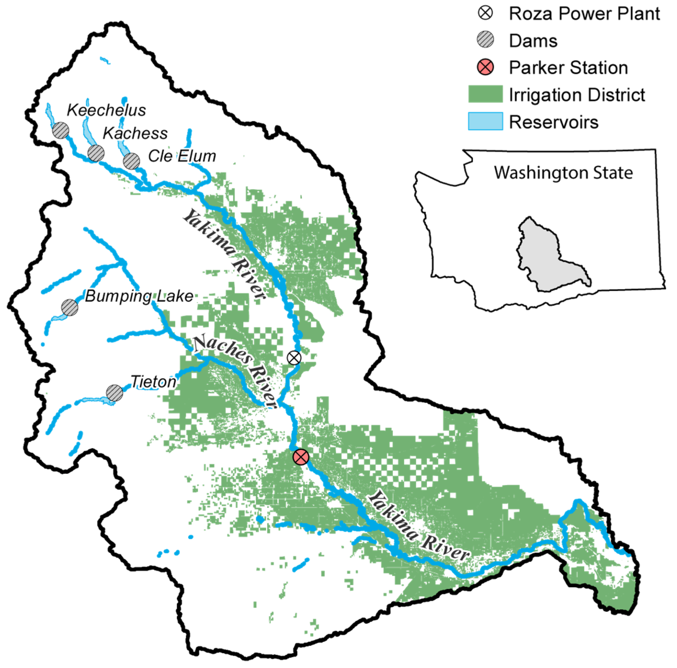
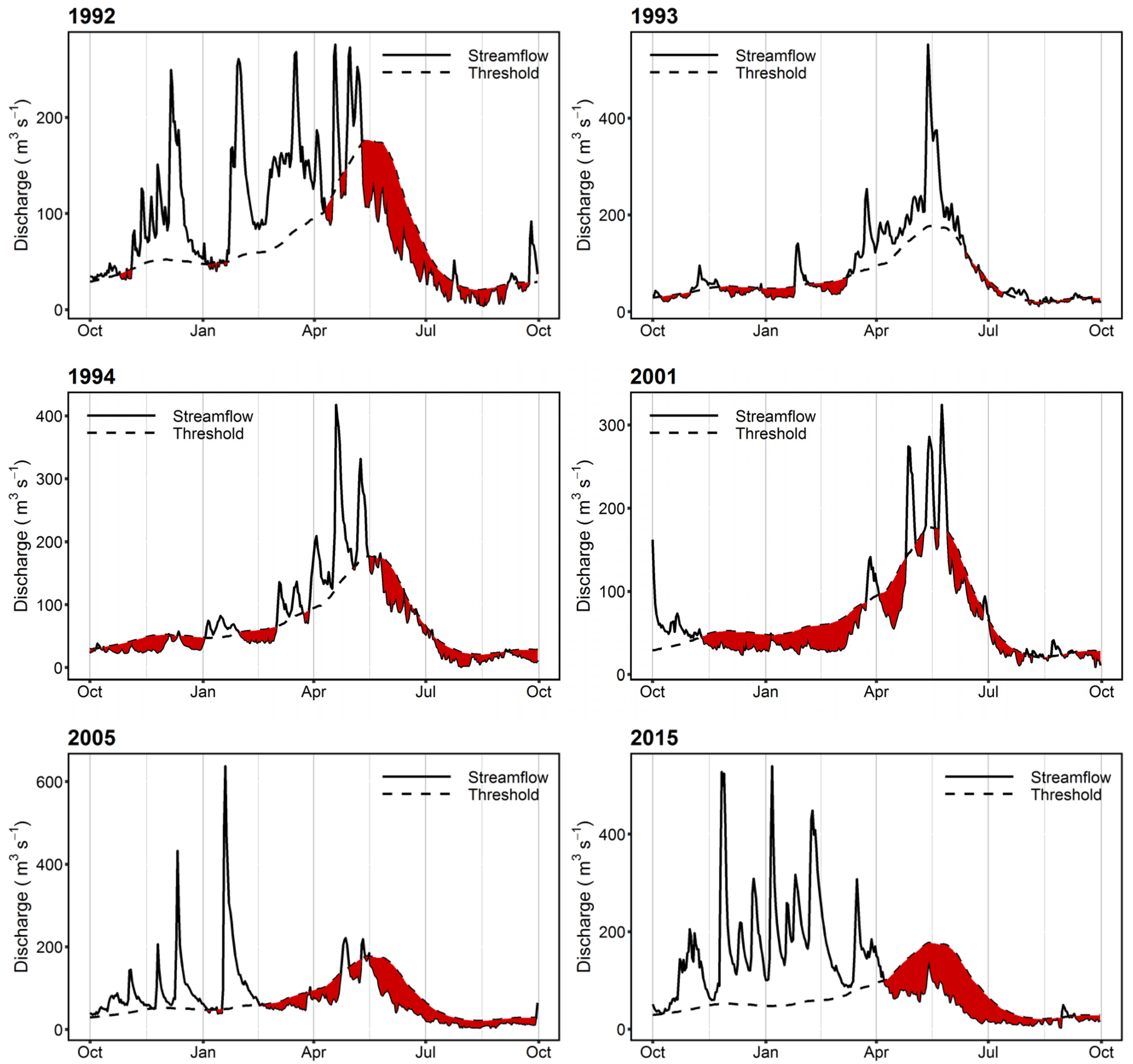
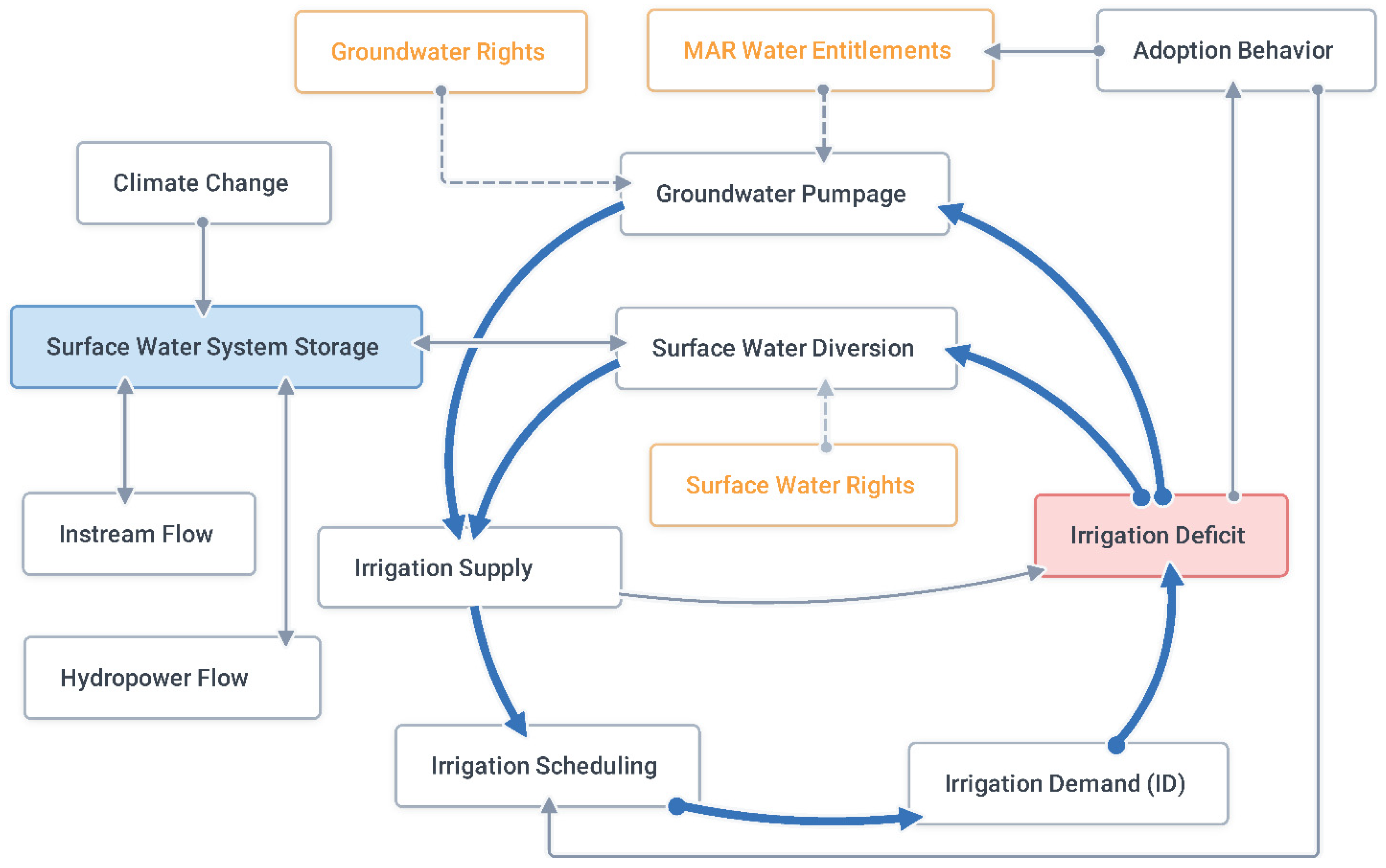
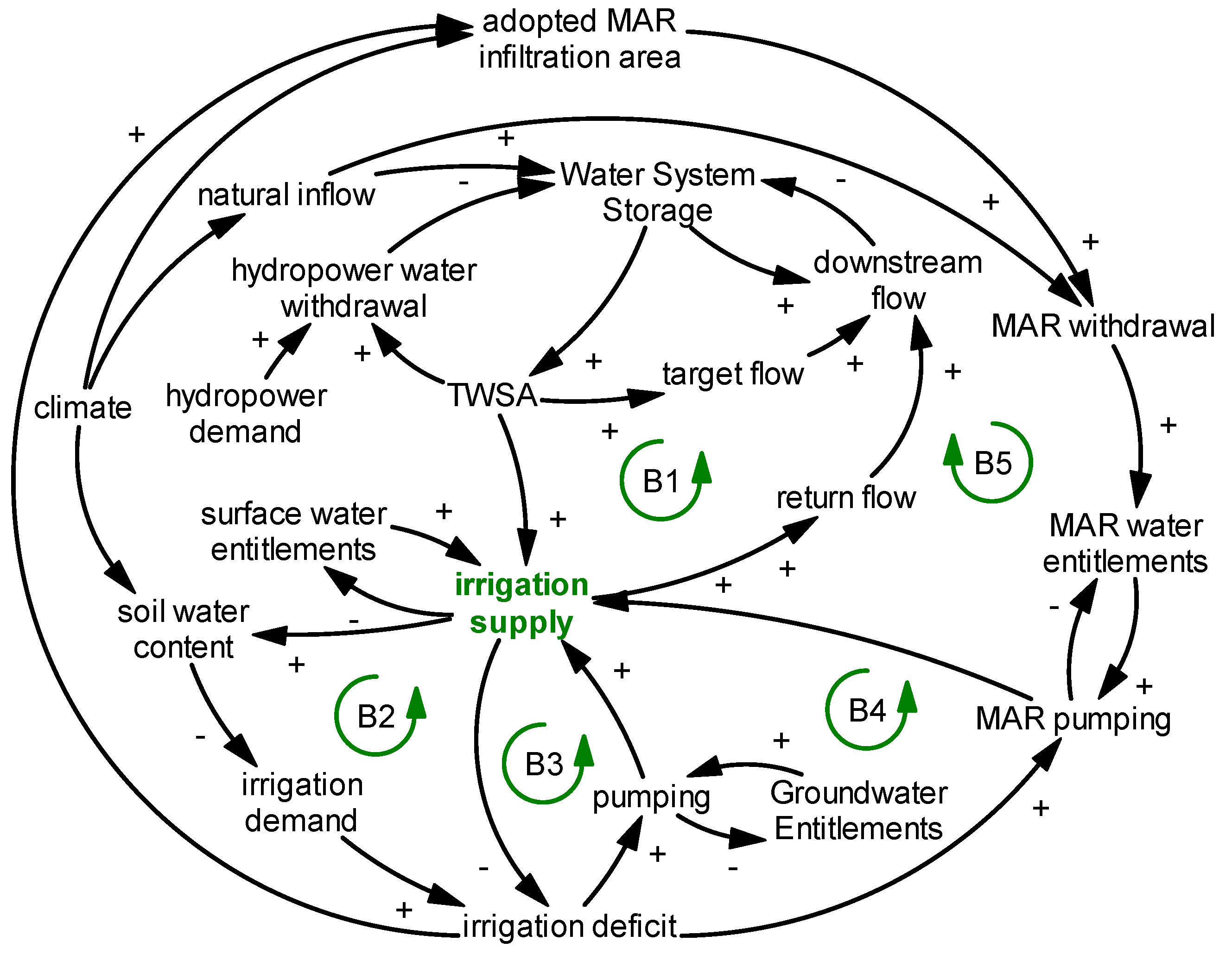
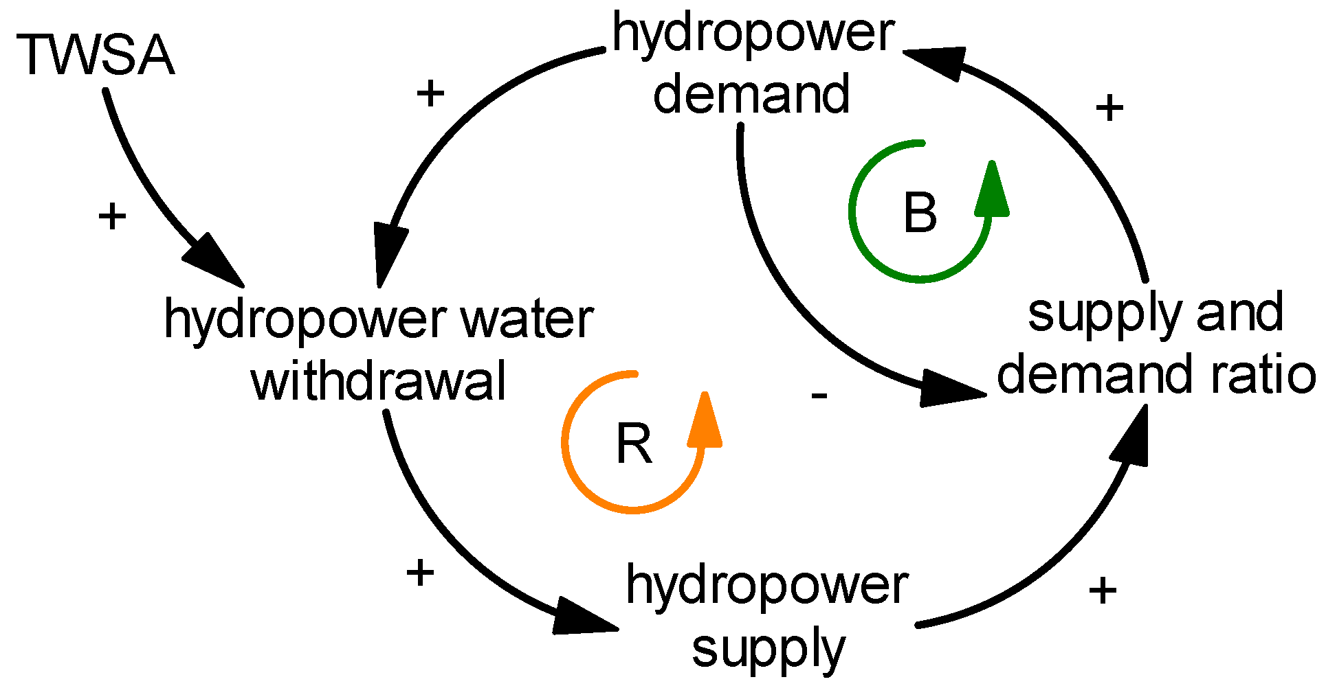
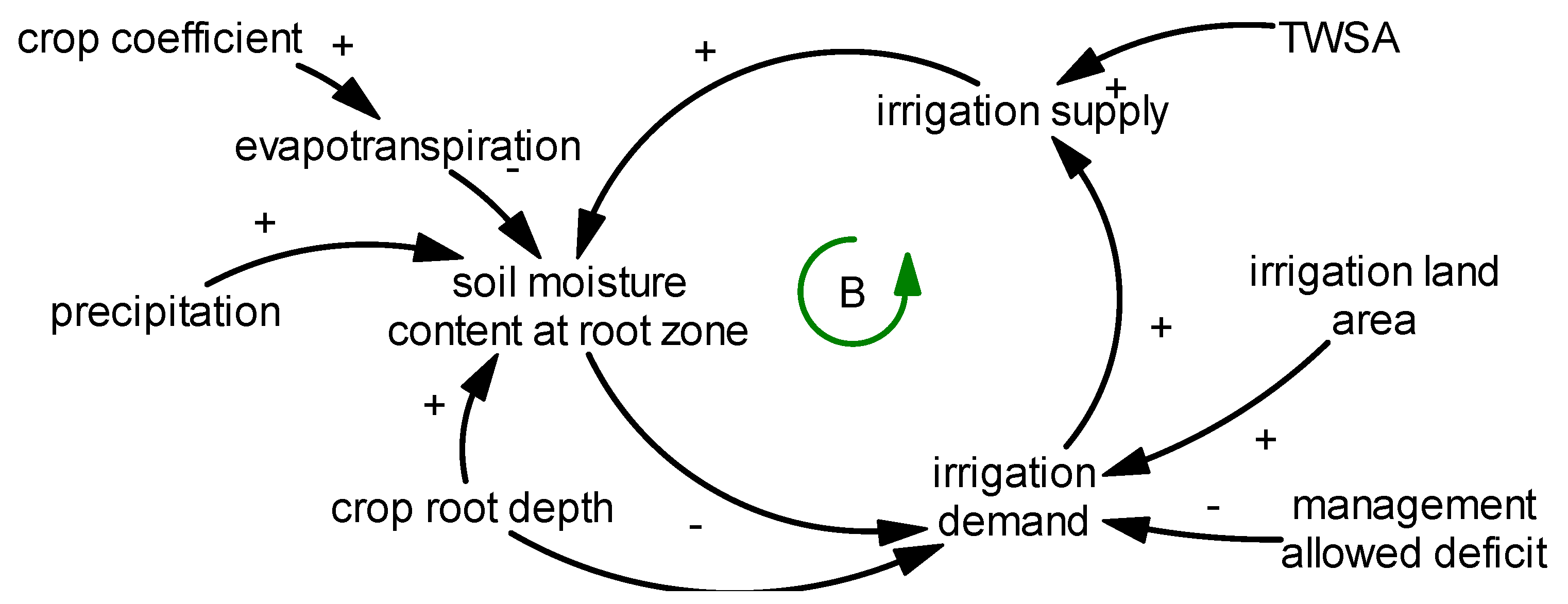
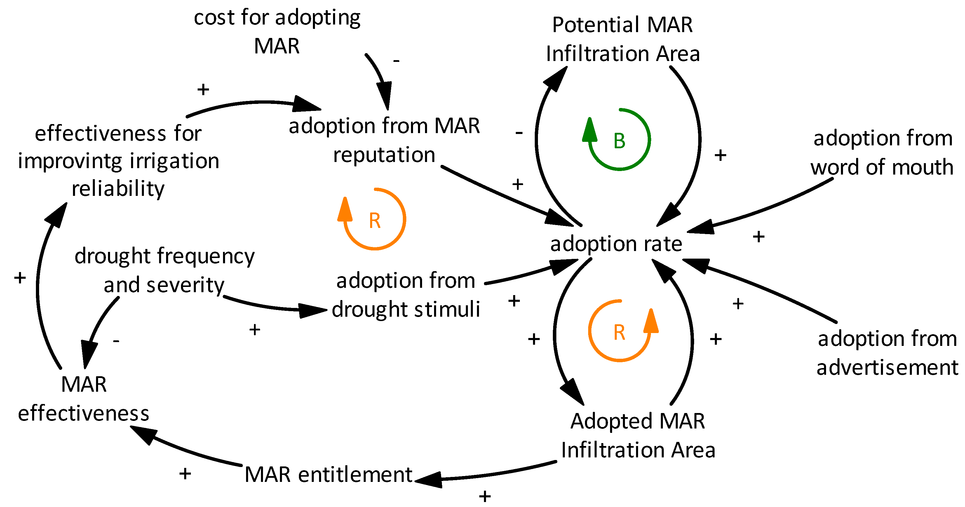
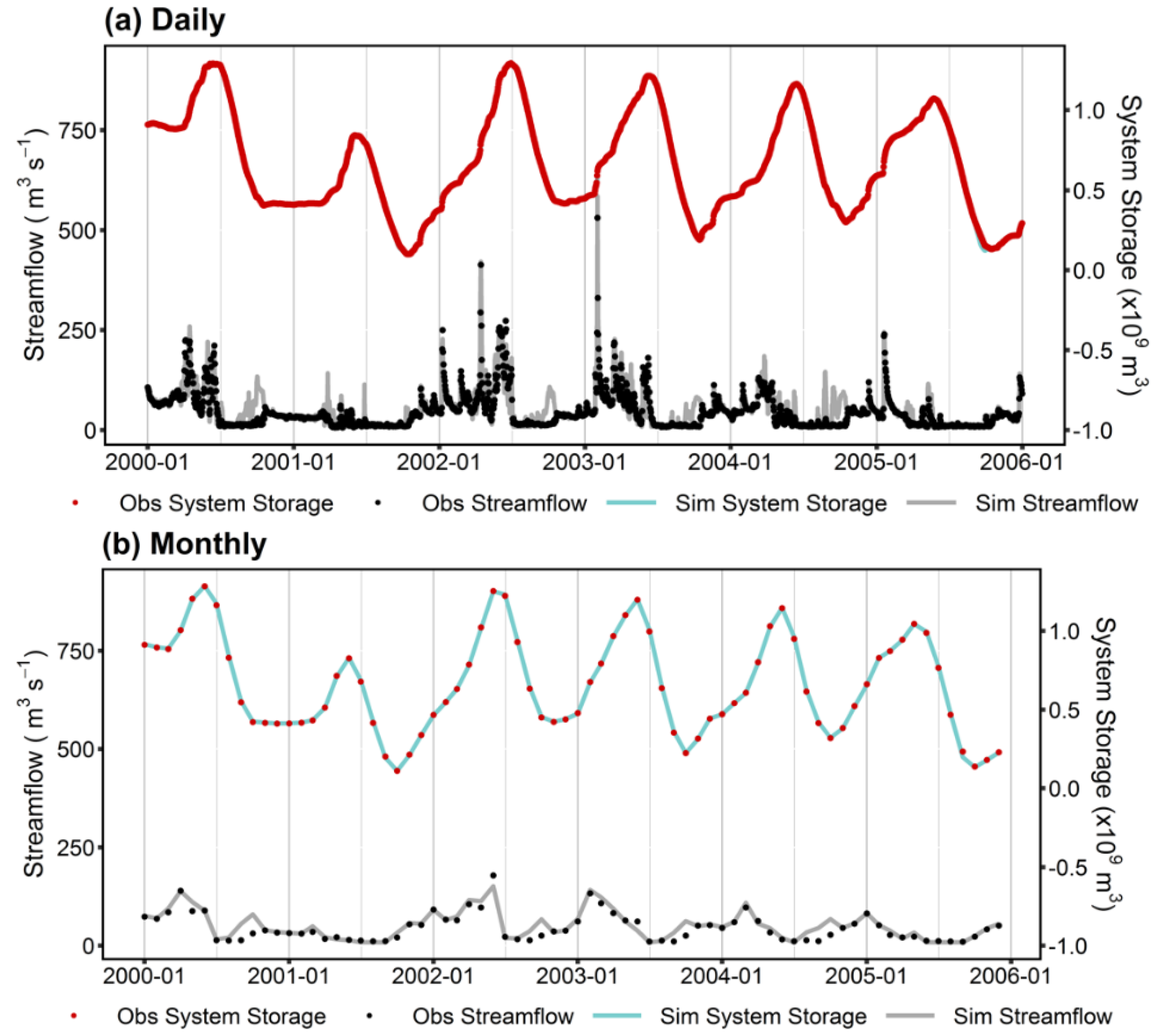
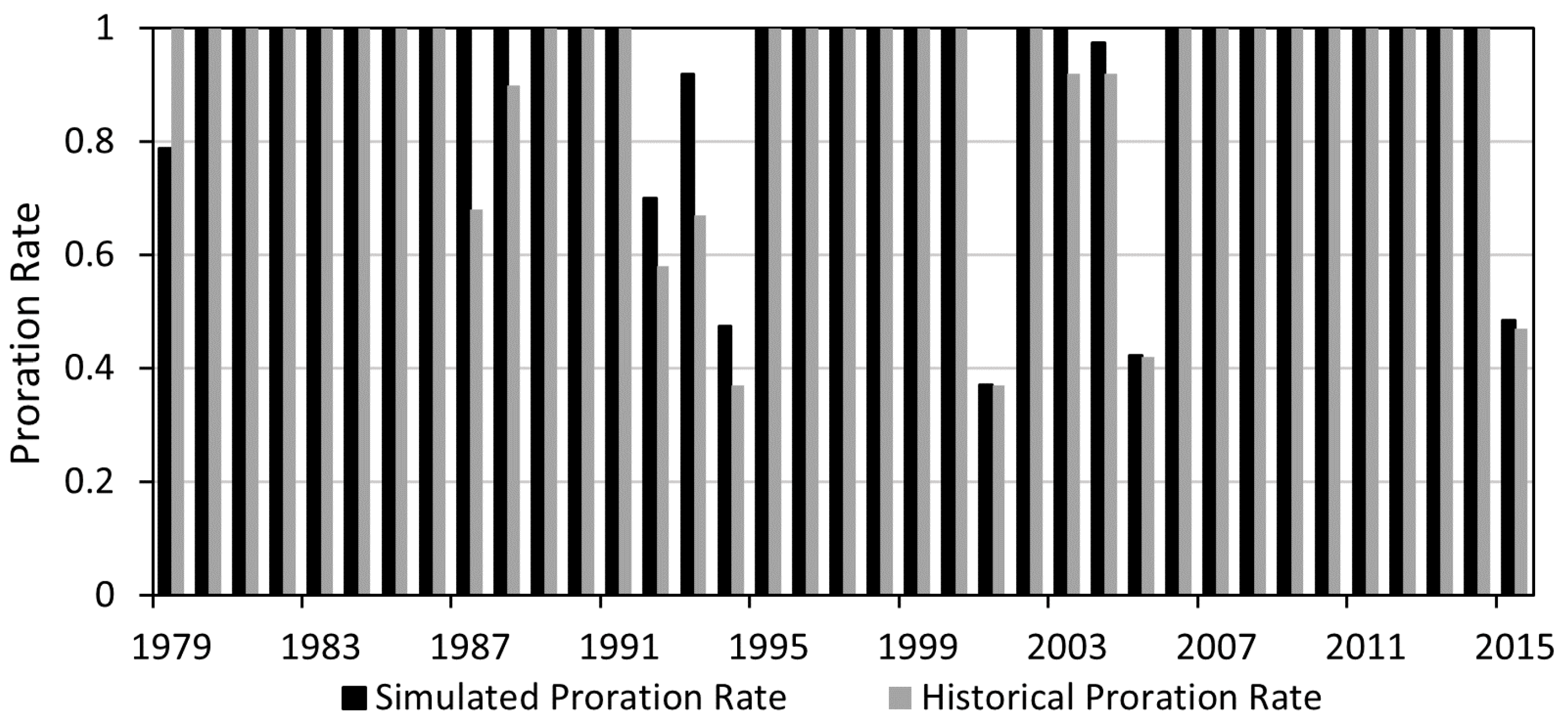
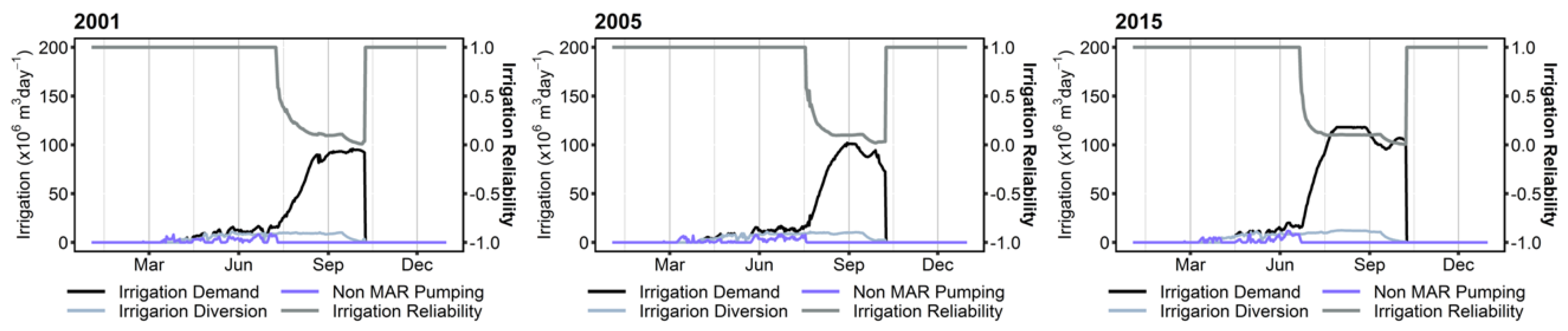
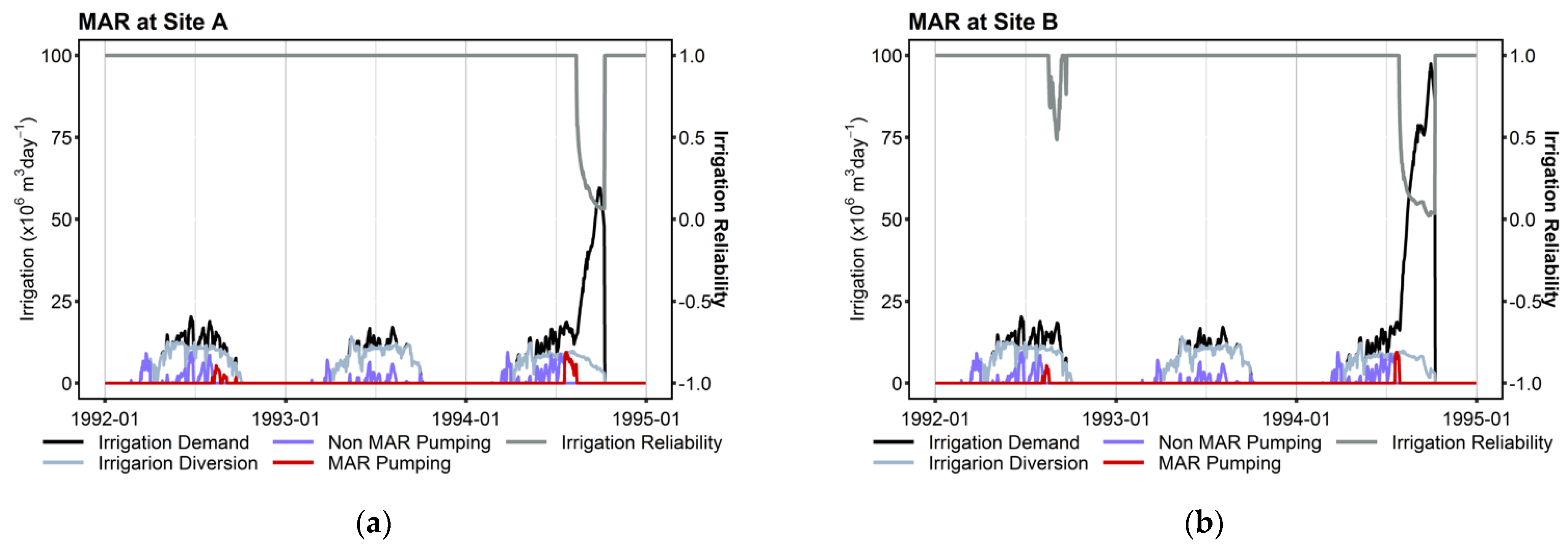
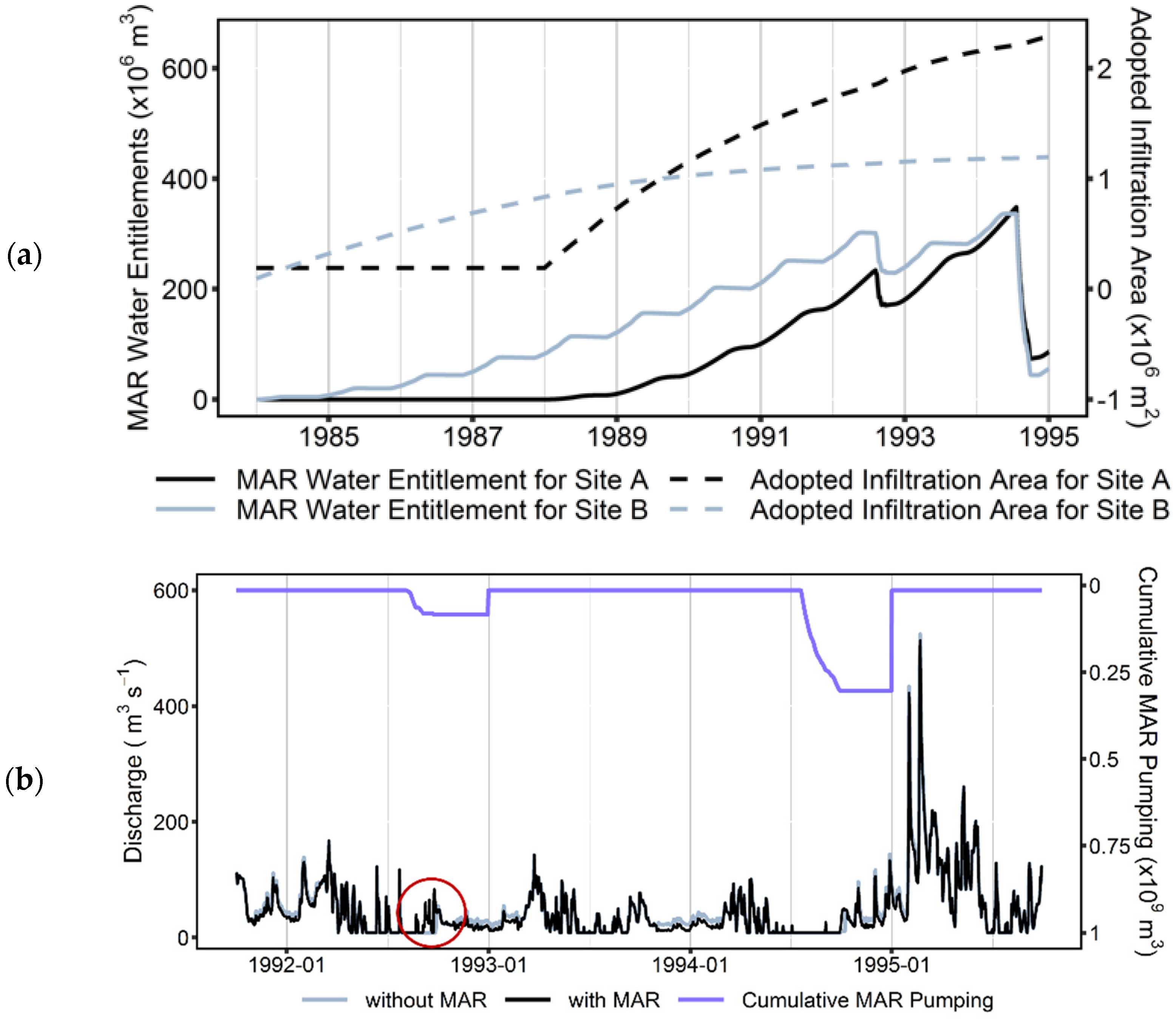
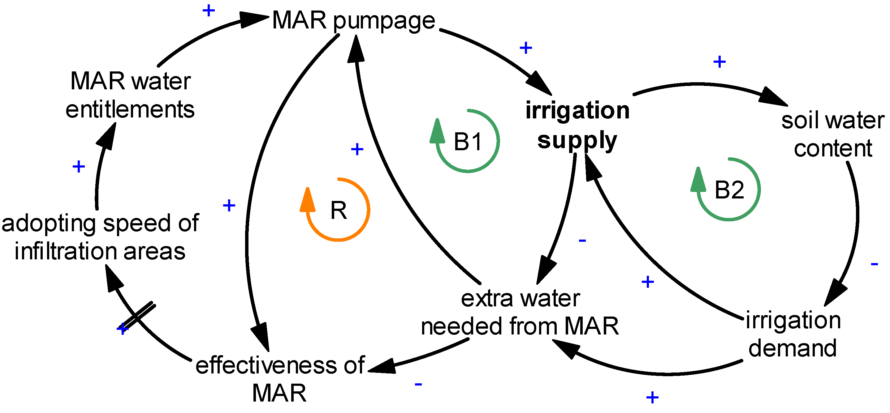
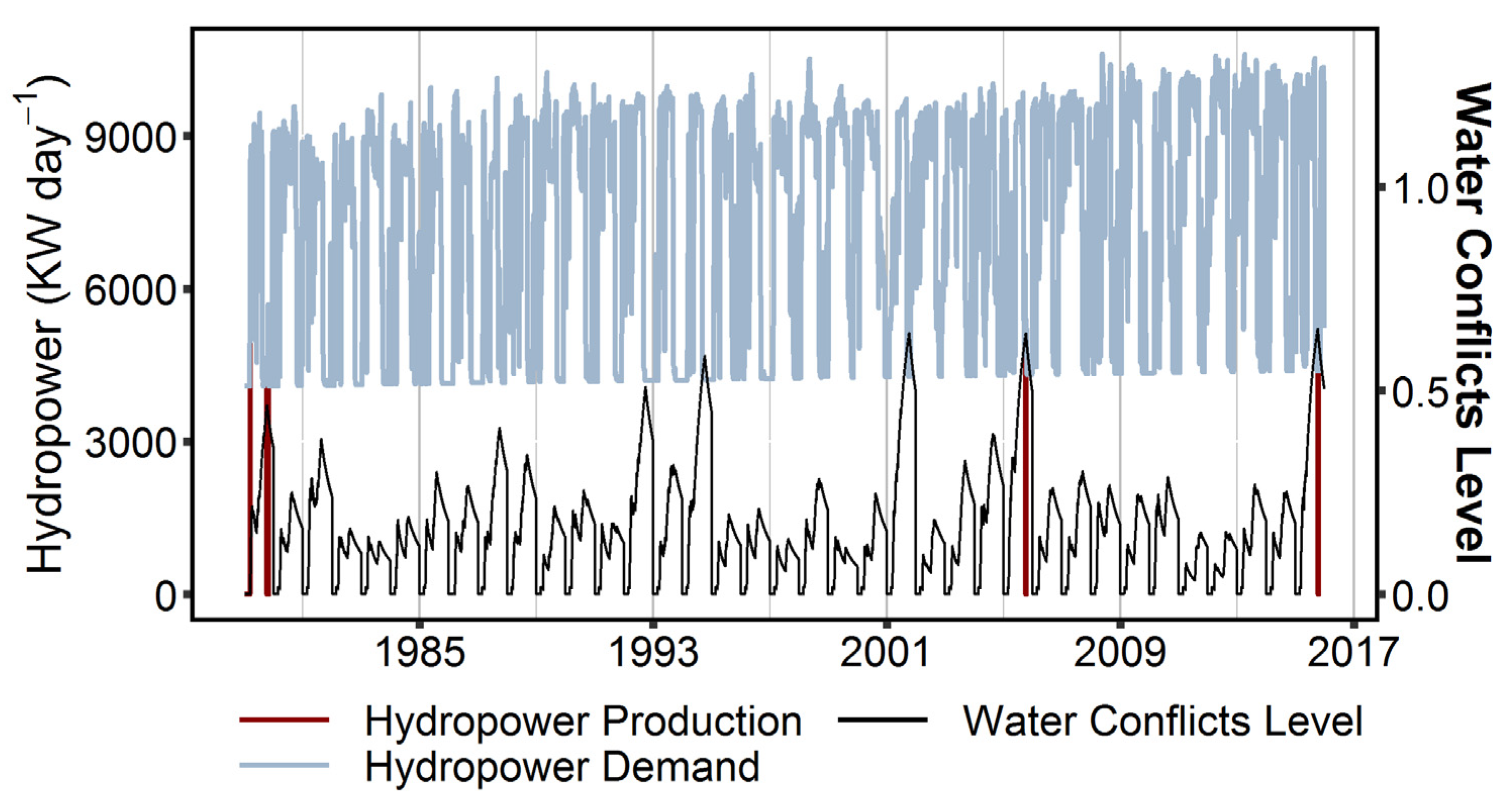
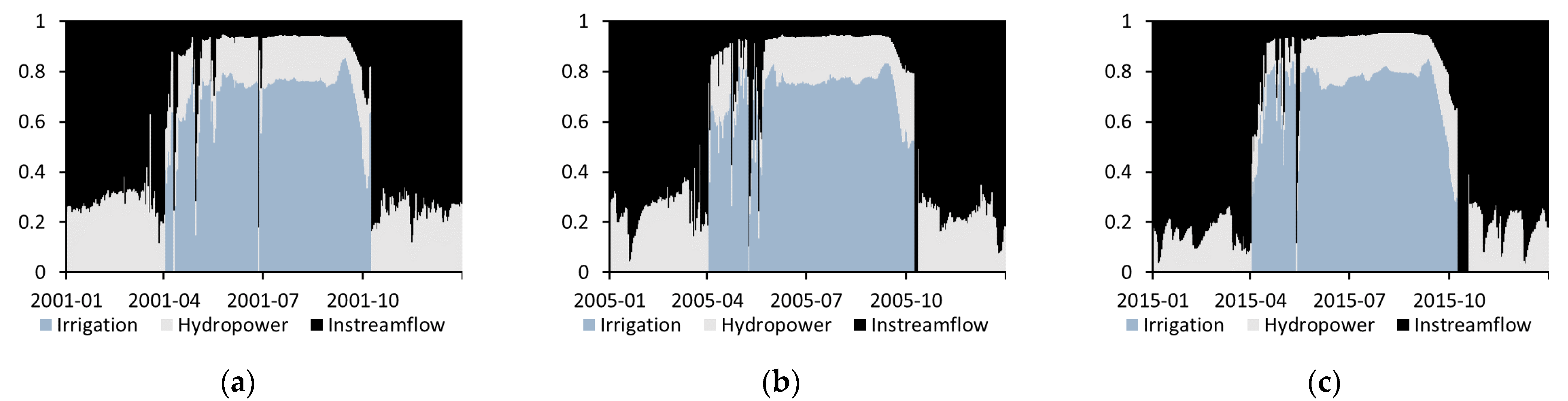
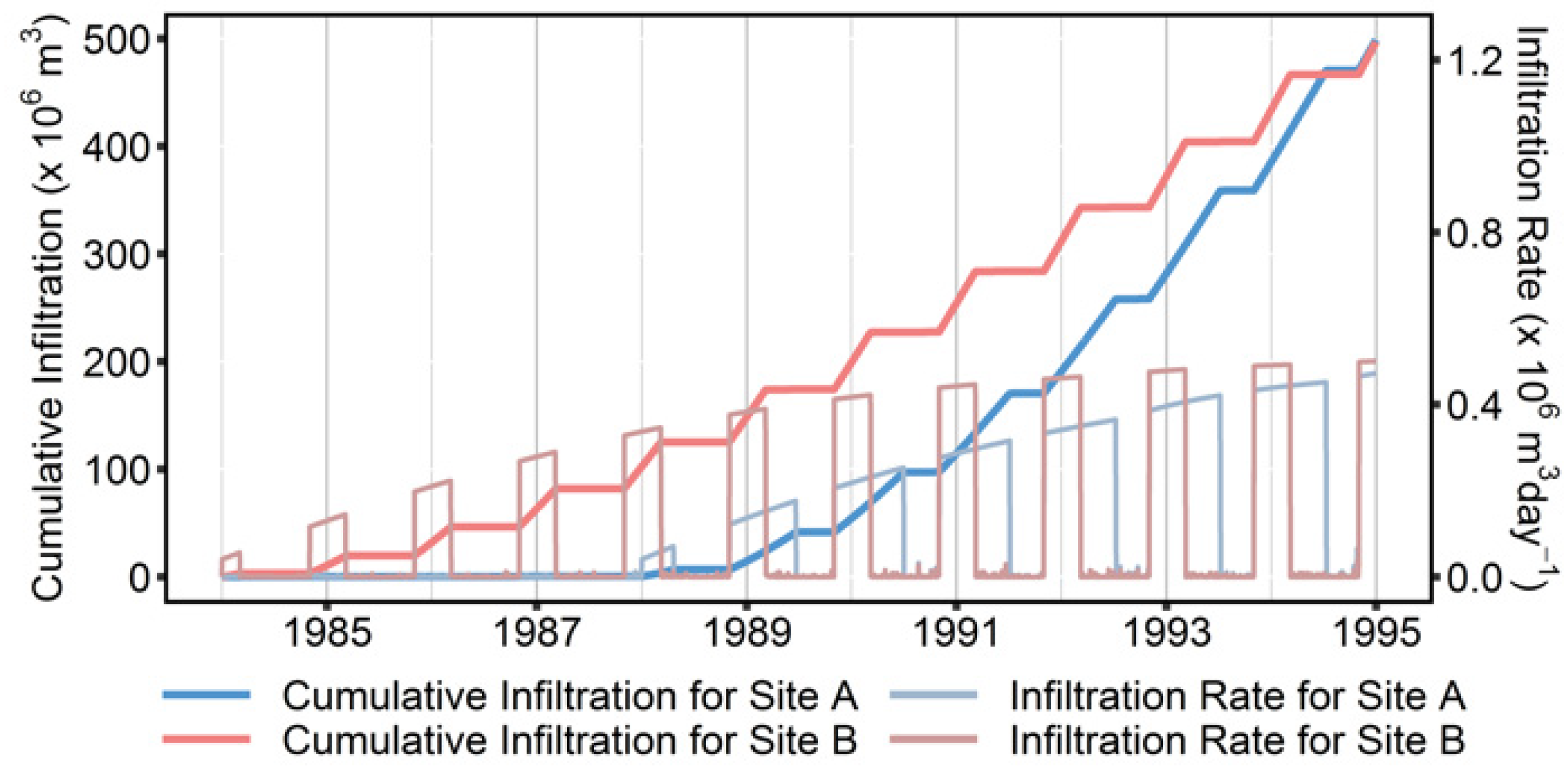
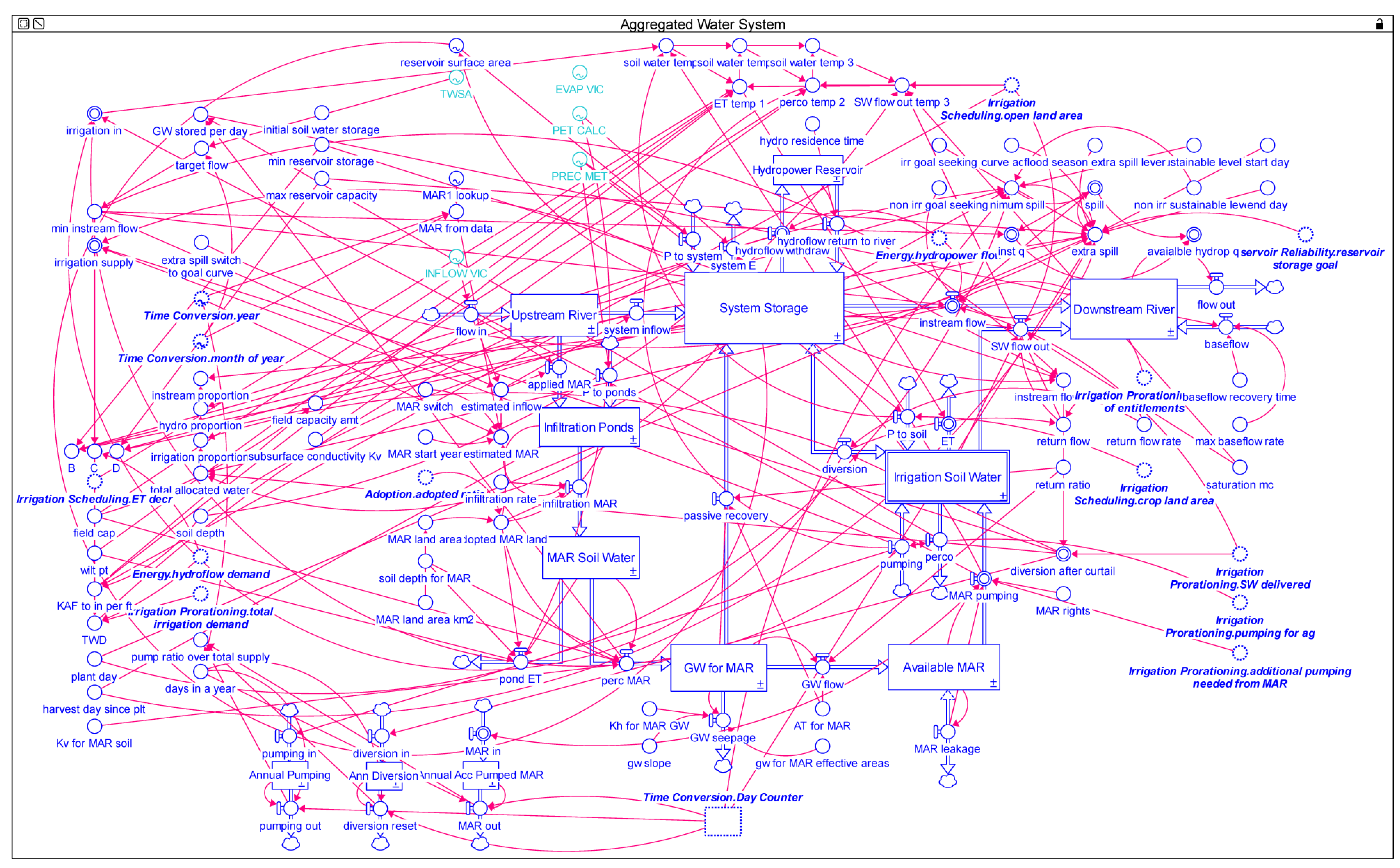
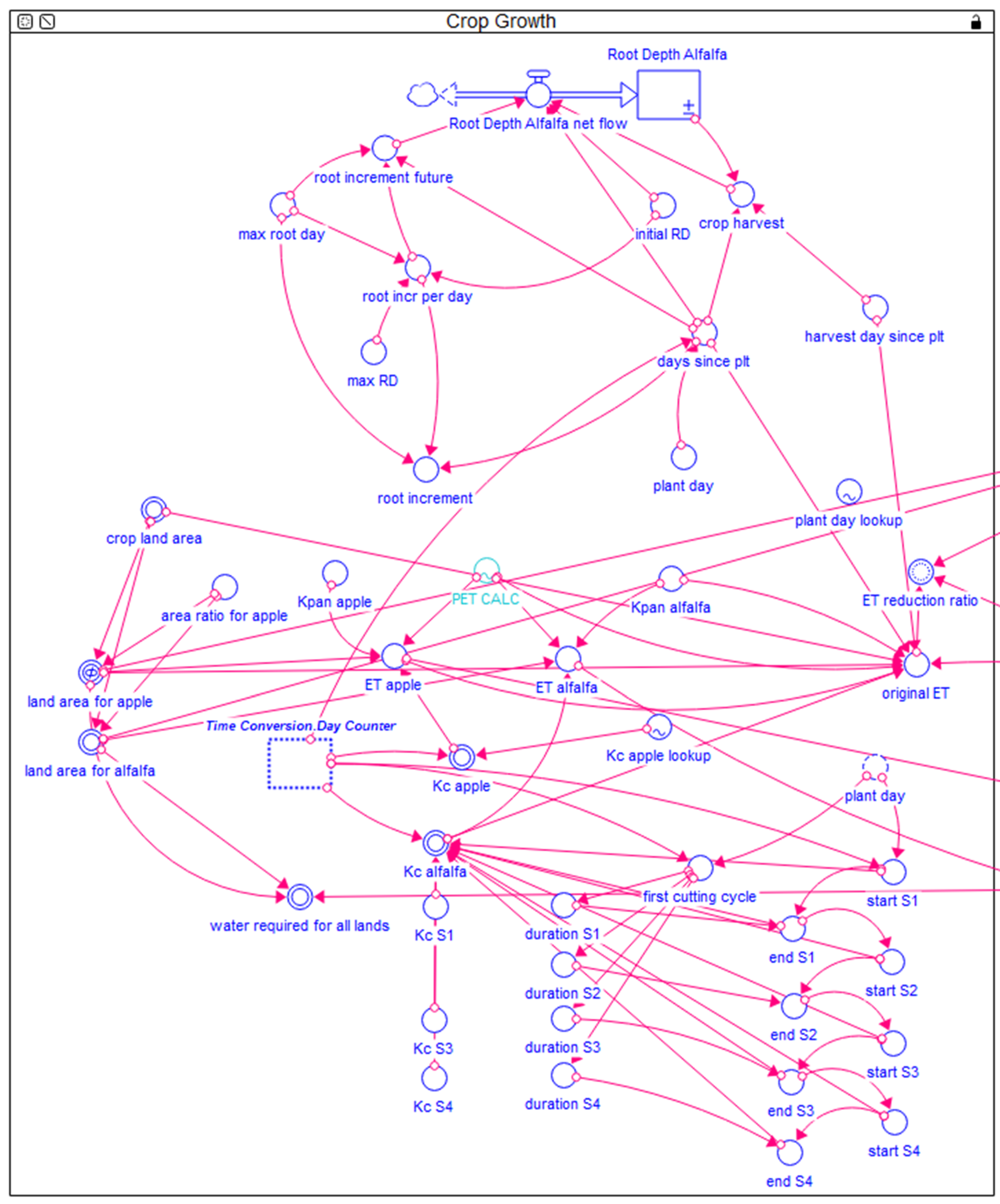
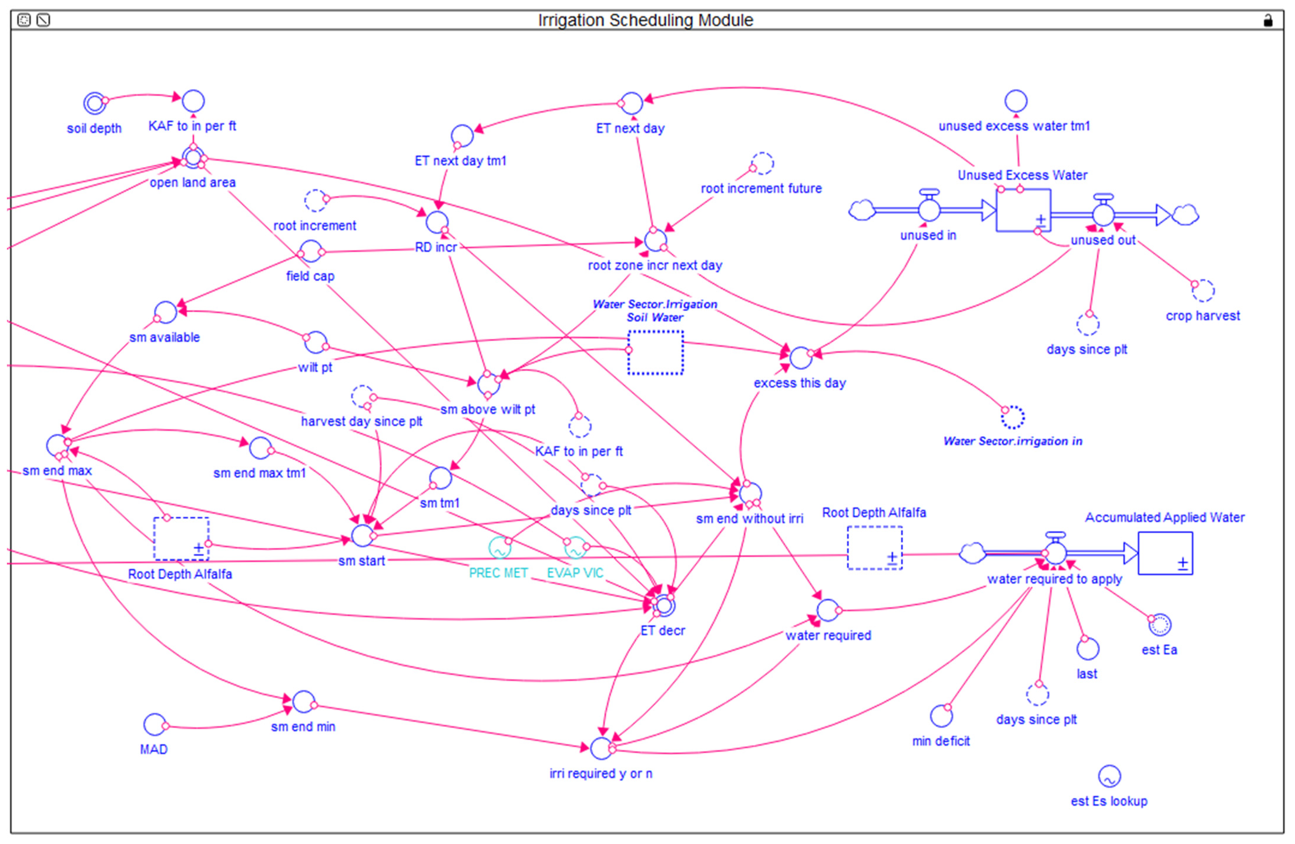
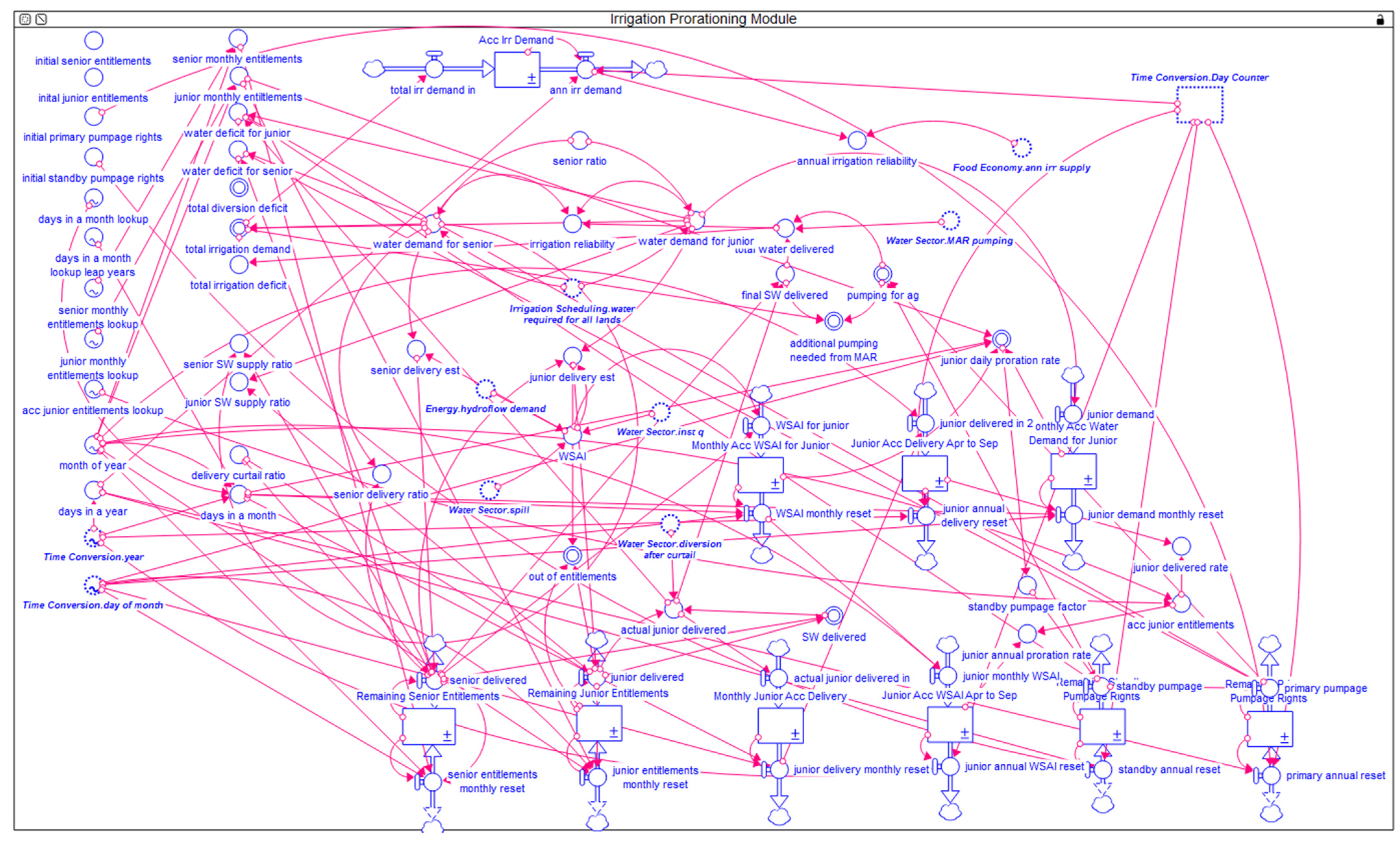
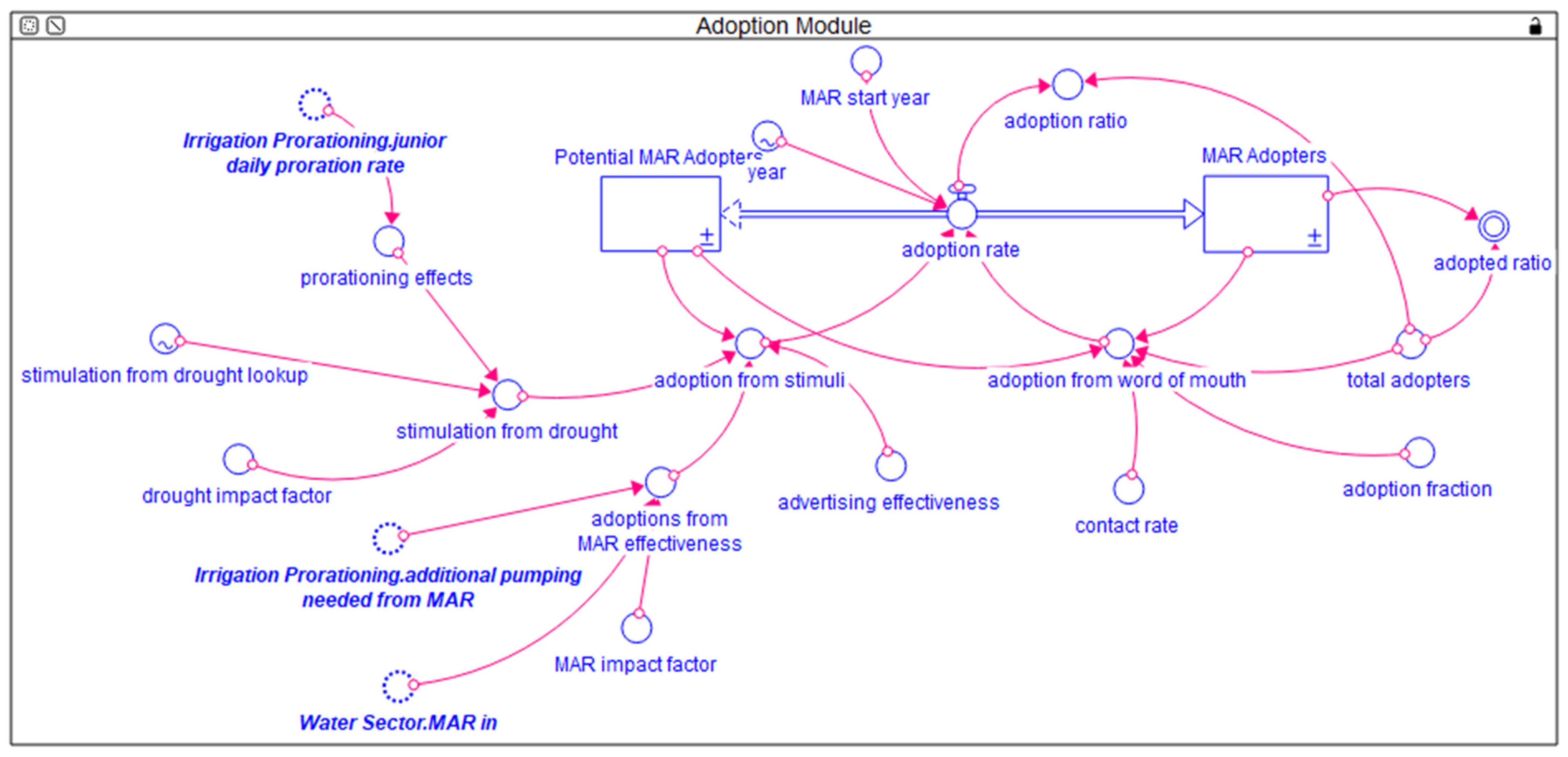
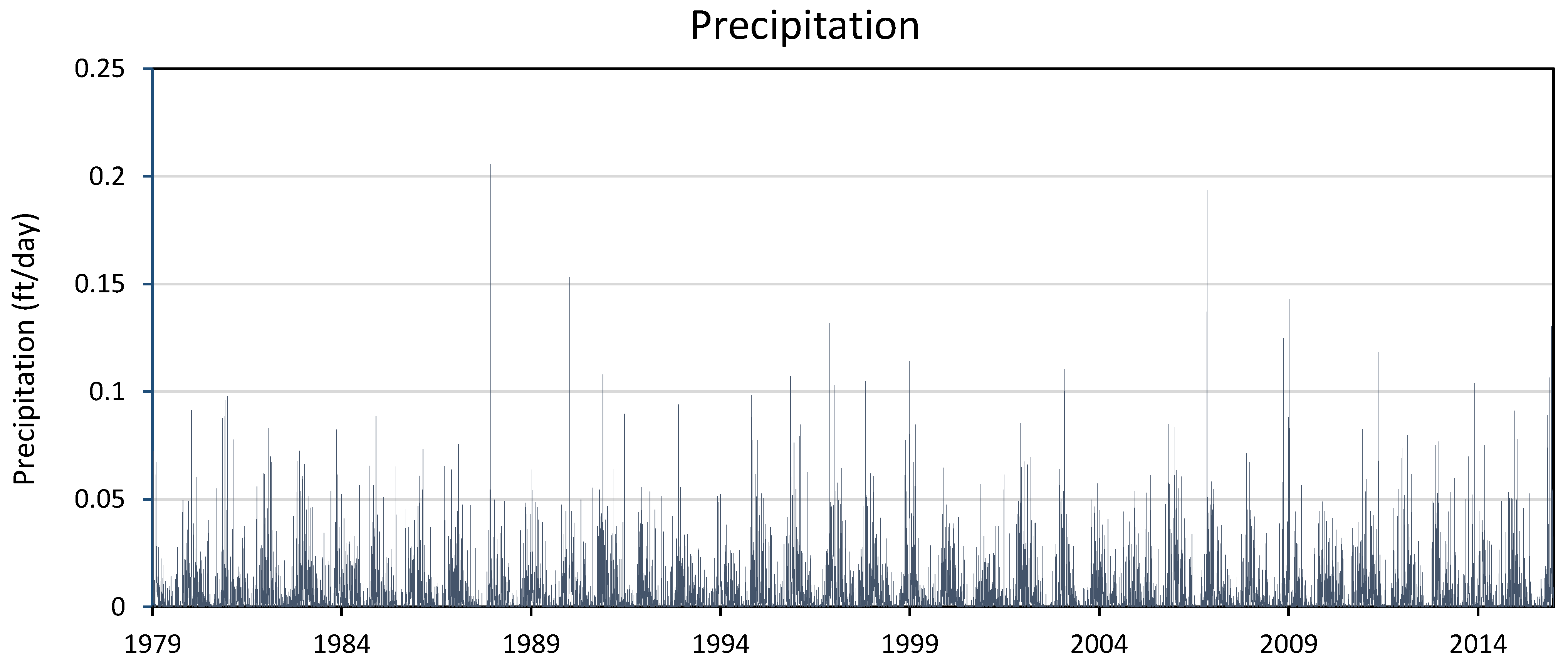
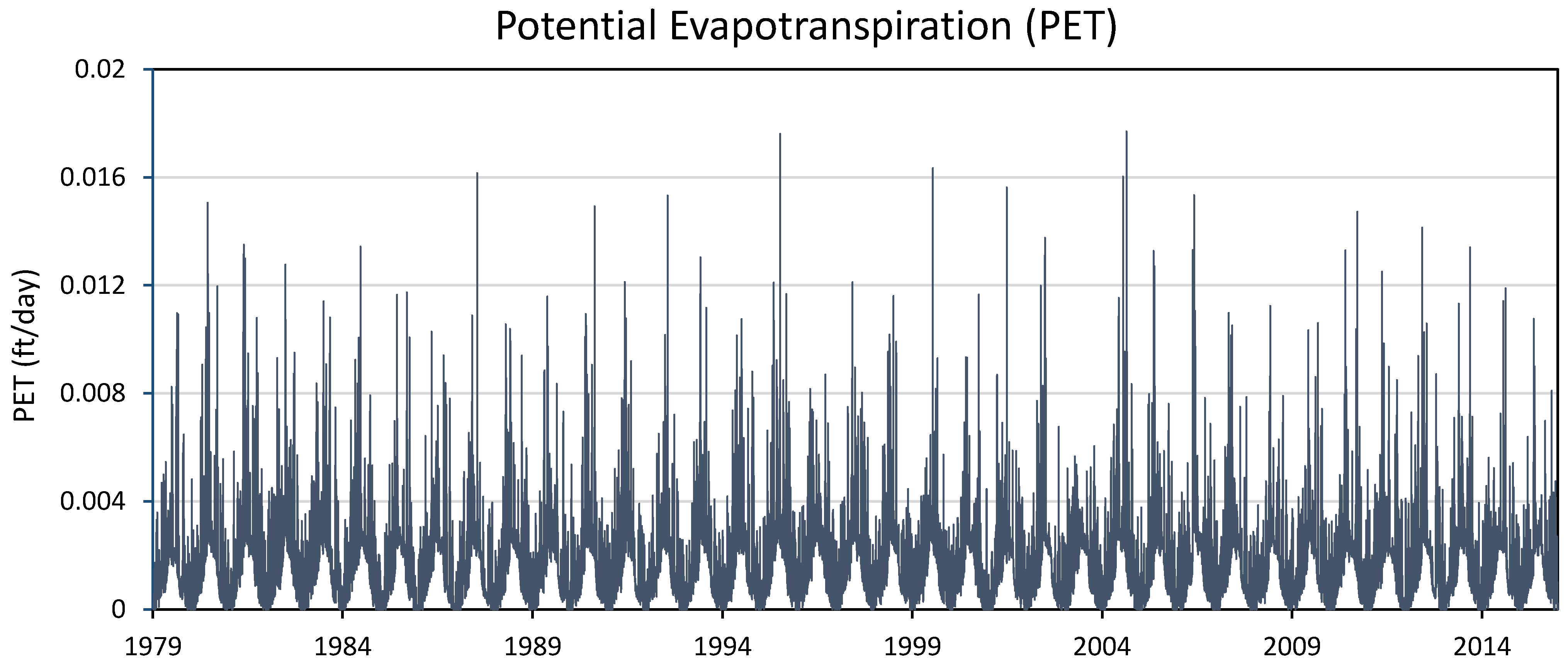
Table 1.
Parameter values for baseline in single drought analysis and for infiltration sites A and B in multi-year droughts analysis.
Table 1.
Parameter values for baseline in single drought analysis and for infiltration sites A and B in multi-year droughts analysis.
| MAR Scenario | Infiltration Area at Full Adoption (km2) | Infiltration Rate (m/day) | Vertical Hydraulic Conductivity (m/day) |
|---|---|---|---|
| Baseline | N/A | 0.43 | 1.52 |
| Site A | 2.4 | 0.21 | 1.52 |
| Site B | 1.2 | 0.43 | 1.52 |
Publisher’s Note: MDPI stays neutral with regard to jurisdictional claims in published maps and institutional affiliations. |
© 2021 by the authors. Licensee MDPI, Basel, Switzerland. This article is an open access article distributed under the terms and conditions of the Creative Commons Attribution (CC BY) license (https://creativecommons.org/licenses/by/4.0/).
Share and Cite
MDPI and ACS Style
Zhao, M.; Boll, J.; Adam, J.C.; Beall King, A. Can Managed Aquifer Recharge Overcome Multiple Droughts? Water 2021, 13, 2278. https://doi.org/10.3390/w13162278
AMA Style
Zhao M, Boll J, Adam JC, Beall King A. Can Managed Aquifer Recharge Overcome Multiple Droughts? Water. 2021; 13(16):2278. https://doi.org/10.3390/w13162278
Chicago/Turabian StyleZhao, Mengqi, Jan Boll, Jennifer C. Adam, and Allyson Beall King. 2021. "Can Managed Aquifer Recharge Overcome Multiple Droughts?" Water 13, no. 16: 2278. https://doi.org/10.3390/w13162278
Note that from the first issue of 2016, this journal uses article numbers instead of page numbers. See further details here.