
Wildfire Impacts on Groundwater Aquifers: A Case Study of the 1996 Honey Boy Fire in Beaver County, Utah, USA


Department of Civil Engineering, University of Colorado Denver, Campus Box 113, P.O. Box 173364, Denver, CO 80217-3364, USA
*
Author to whom correspondence should be addressed.
Water 2021, 13(16), 2279; https://doi.org/10.3390/w13162279
Submission received: 30 June 2021
/
Revised: 4 August 2021
/
Accepted: 17 August 2021
/
Published: 20 August 2021
(This article belongs to the Section Hydrology)
Abstract
:It is well known that wildfires destroy vegetation and form soil crusts, both of which increase stormwater runoff that accelerates erosion, but less attention has been given to wildfire impacts on groundwater aquifers. Here, we present a systematic study across the contiguous United States to test the hypothesis that wildfires reduce infiltration, indicated by temporary reductions in groundwater levels. Geographic information systems (GIS) analysis performed using structured queried language (SQL) categorized wildfires by their proximity to wells with publicly available monitoring data. Although numerous wildfires were identified with nearby monitoring wells, most of these data were confounded by unknown processes, preventing a clear acceptance or rejection of the hypothesis. However, this analysis did identify a particular case study, the 1996 Honey Boy Fire in Beaver County, Utah, USA that supports the hypothesis. At this site, daily groundwater data from a well located 790 m from the centroid of the wildfire were used to assess the groundwater level before and after the wildfire. A sinusoidal time series adjusted for annual precipitation matches groundwater level fluctuations before the wildfire but cannot explain the approximately two-year groundwater level reduction after the wildfire. Thus, for this case study, there is a correlation, which may be causal, between the wildfire and temporary reduction in groundwater levels. Generalizing this result will require further research.
1. Introduction
One of the biggest challenges in environmental hydrology is to prevent and control damage caused by wildfires. As of late, wildfires are occurring more frequently and with greater intensity [1,2,3,4,5,6] resulting from climate change, power line construction within heavily wooded areas, and the lack of forest management practices [7]. This increase in frequency and intensity is important for environmental hydrology because wildfires trigger flash floods [8,9], debris flows [1,10], and erosion [4,5,11,12], although erosion per area decreases with area as larger catchments provide more opportunity to trap eroded sediment [10].
The hydrologic impacts of wildfires result from a number of interacting processes. During these wildfires, ash mixes with topsoil to form a water-repellent layer, which makes the soil more impervious [11,13,14,15,16]. This imperviousness increases runoff from wildfire-affected areas, accelerating erosion and causing large amounts of soil loss. The literature also emphasizes that wildfire can induce, enhance, or destroy soil water repellency [8,10,12,14,15,16,17,18,19], which controls the interaction of water and soils. More recent studies have recognized how wildfires disrupt soil-dwelling organisms [20], for example termites [21], which provide a number of ecosystem services including the creation of macropores that often control infiltration [14,21]. The net result of wildfire-induced changes in ash layers, soil water repellency, and macropores is decreased infiltration [1,8,9,11,12,13,14,15,16,18,22]. On this key point the literature is nearly unanimous, although there are a number of reports where fires increased infiltration rates [18,23], an unusual observation that presumably results from the variable effects of wildfire on soil water repellency.
The focus of much research related to post-wildfire hydrology has examined the physical and chemical change of the upper-most layer of soil, topsoil. Laboratory evidence as shown by Moody et al. [24] showed that lowered hydraulic conductivity, which controls the movement of water through porous media, depends on the adsorption capacity of the wildfire-affected soil and specifically its ability to retain combusted organic materials (ash, soot, charcoal, etc.). The work of Beatty and Smith [25] adds that fractional wettability, the surface area of soil that physically contacts water, is greatly reduced within wildfire-affected materials. As a result, soils with both higher adsorption capacity and lower fractional wettability tended to have lower hydraulic conductivity. Cawson et al. [26] believe the relationships between soil heating and soil water repellency are strong in the laboratory, although few studies test those relationships under natural conditions.
Although many studies have focused on post-wildfire hydrology, less attention has been given to the impact of wildfires on groundwater aquifers and specifically on groundwater levels. With regard to groundwater chemistry, the few available studies report mixed results. Giambastiani et al. [23] reported improved groundwater quality, specifically a reduction in salinity following a wildfire in a coastal pine forest above an unconfined sandy aquifer. In contrast, Mansilha et al. [27] reported degraded groundwater quality after a wildfire in a peri-urban area that resulted in elevated concentrations of metals and polycyclic aromatic hydrocarbons (PAHs). Interpolating these results, Dimitriadou et al. [28] found that a wildfire above a thick vadose zone had essentially no impact on groundwater quality.
With regard to groundwater quantity, a number of recent studies pointed out that wildfire could affect groundwater levels [22,23], presumably through the changes in infiltration noted above. Tsinnajinnie et al. [6] found that perennial and intermittent springs enhance post-fire watershed recovery, which again points to the importance of groundwater aquifers. Pham et al. [29] performed a meta-analysis of groundwater levels in 13,433 wells, finding a correlation with wildfires that is strongest in the first year and persists for up to four years. This finding is consistent with that of Schneider et al. [30], who constructed water balance models for wildfire-impacted catchments in the San Juan Mountains of Colorado, finding increased runoff (corresponding to decreased infiltration) in the first few years after the wildfire.
However, to our knowledge, no study has yet to establish a correlation between wildfire and groundwater levels at a particular site. Therefore, the current study addressed the following question: can one detect changes in groundwater levels at a particular well before and after a wildfire? Knowing how aquifers may be affected by wildfires can help to answer three questions: (1) is there a significant change in soil infiltration after a wildfire? (2) Is soil permeability restored to pre-wildfire levels given enough time? (3) What long-term effects may a wildfire have on groundwater?
2. Methods
This study considers spatial and temporal data on wildfires, groundwater levels, and annual precipitation. Three criteria were applied to identify wildfires with nearby monitoring wells. First, groundwater wells must be located within the perimeter of the burn area of the wildfire, assumed to be approximately circular, centered at the wildfire centroid, with area approximately equal to the maximum for its wildfire size class. Second, groundwater data must include daily or weekly groundwater levels for at least three years before and after the wildfire. Third, groundwater data must be free of confounding by unknown processes; in other words, the analysis only considers sites where groundwater levels could be described by a sinusoidal model for annual fluctuations adjusted by annual precipitation for at least three years before the wildfire. Each site was examined on a case-by-case basis to determine which groundwater data are suitable for in-depth modeling.
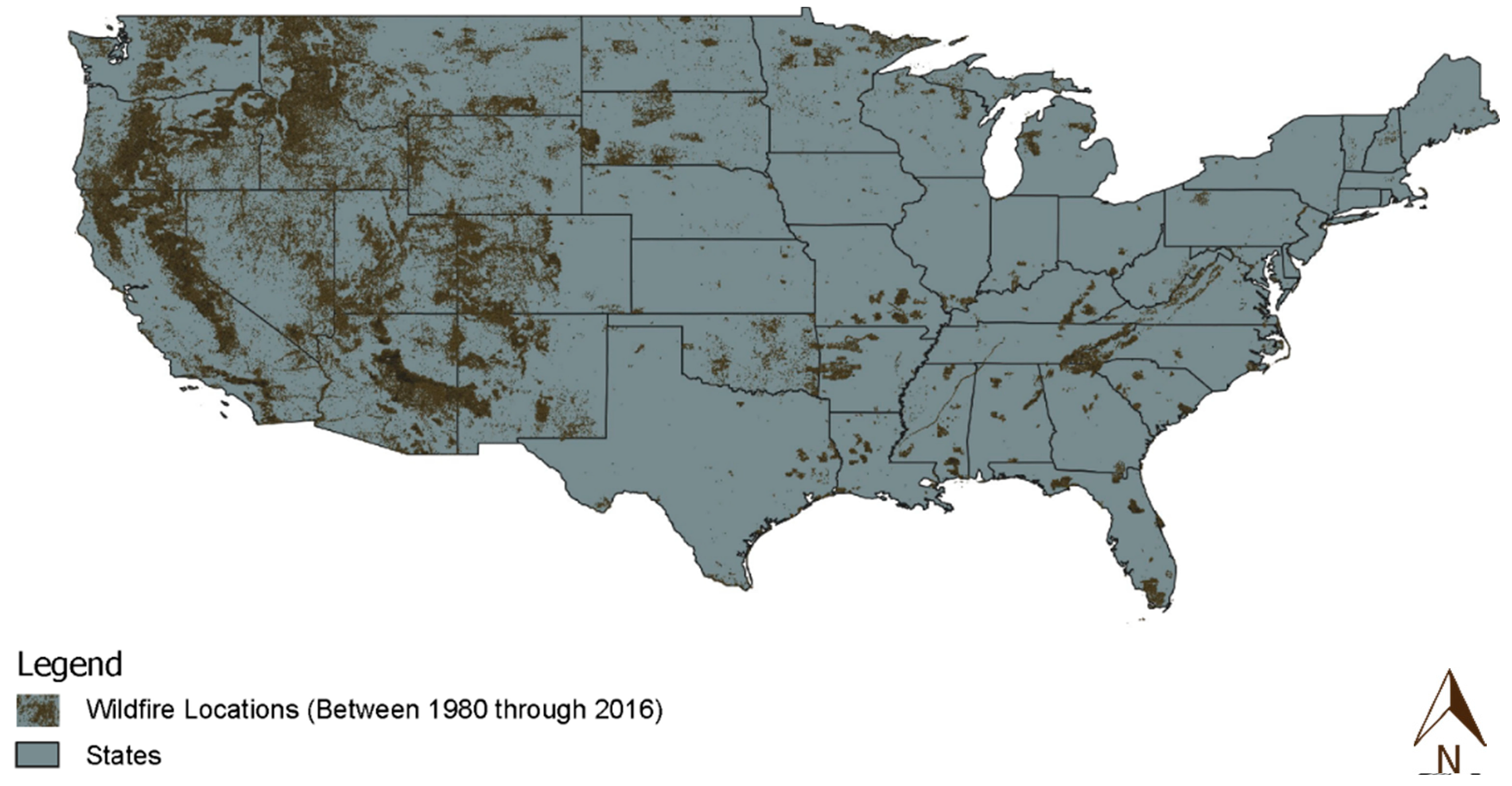
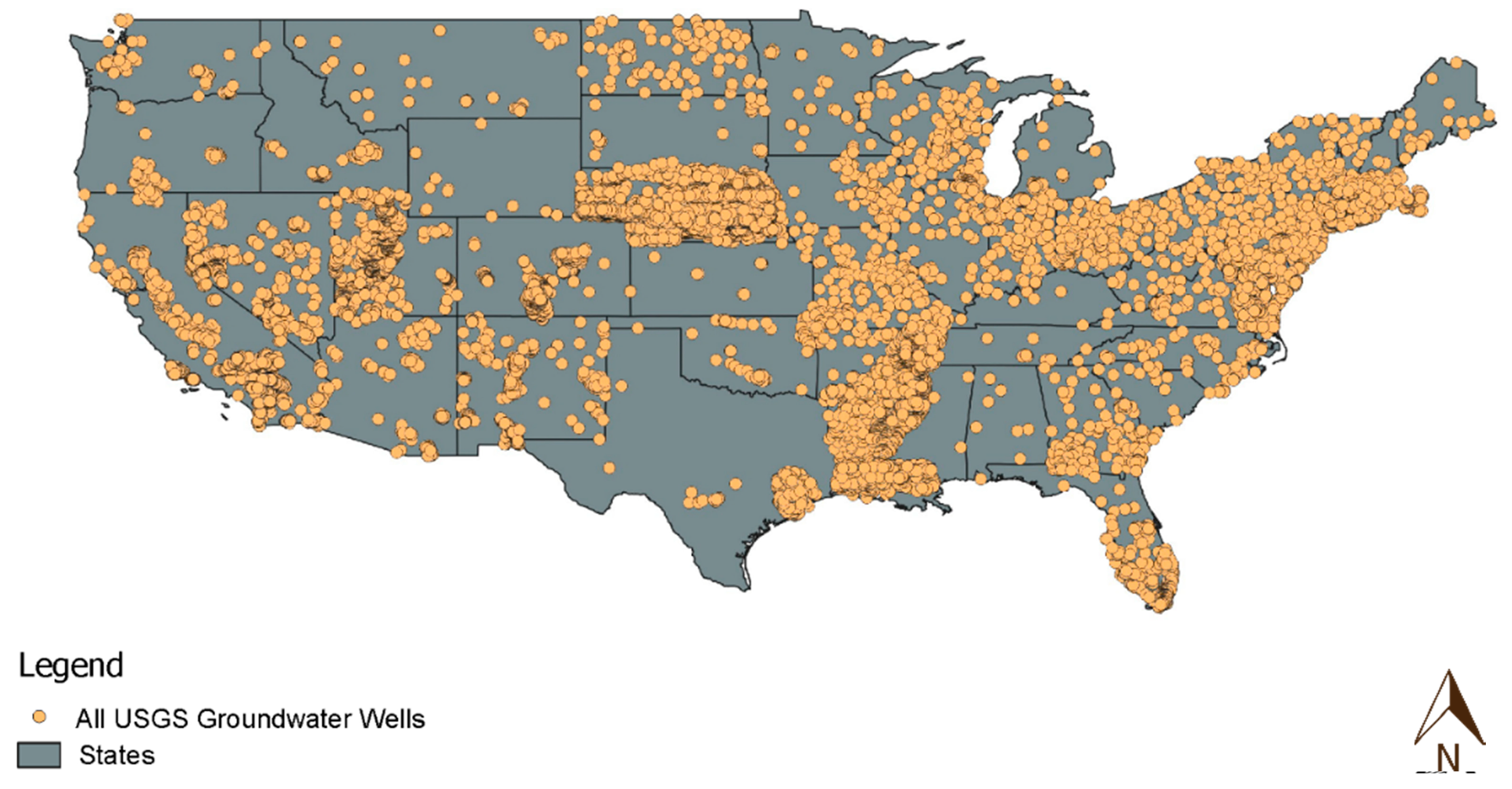
Since this study requires wildfires with nearby groundwater wells, publicly available geographic information system (GIS) datasets were employed to calculate the distance between each wildfire centroid and the nearest monitoring well. Specifically, two GIS datasets were utilized for the purposes of this study. First, the dataset Wildfire_all_1980_2016 [31] is a shapefile and point dataset providing approximate coordinates for the centroids of all recorded wildfires within the contiguous United States from 1980 to 2016 (Figure 1). The data also include descriptive information about each wildfire including its name, size class, date started, and the date contained. A total of 595,158 wildfires are included in this dataset. Second, the dataset USGS_Monitoring_Wells [32] is a shapefile and point dataset providing coordinates for all USGS monitoring wells within the contiguous United States (Figure 2). The data also include descriptive information about the vertical datum used to measure well depths. A total of 17,754 groundwater wells are included in this dataset.
The distance between each wildfire centroid and the nearest well was calculated using the software PostGIS. Using structured query language (SQL), the two GIS datasets were translated into a common coordinate system, North American Datum 1983 (NAD 83), and results were sorted by wildfire size class. Seven different size classes of wildfires exist based on total burn area [33]. Class A and B fires, corresponding to total burn areas less than 4.0 ha (10 ac), were assumed to be too small to impact groundwater infiltration and were therefore excluded, reducing the number of wildfires considered to 43,790. Details on the other size classes C-G are provided in Table 1. The maximum area of each size class was used to calculate an equivalent radius, which was then converted into degrees in order to use a spherical distance query in PostGIS (Table 1). This query identified monitoring wells within the equivalent radius (expressed in degrees) of each wildfire centroid. Assuming a spherical Earth, in the north-south direction, 1° = 111.3 km. In the east-west direction, the conversion from degrees to distance depends on latitude. For the latitude of 38°20′20″, corresponding to the case study discussed below, 1° = 87.3 km. Accordingly the search areas are slightly elliptical with a major axis in the north-south direction. This query was repeated and modified for the five wildfire size classes C-G as shown in the Appendix A.
This spherical distance query identified monitoring wells that met the first criterion, to be within a wildfire burn area. Checking the second and third criteria (for sufficiently long and well-behaved data) requires a manual check that comprises two steps. First, the USGS website (https://waterdata.usgs.gov/nwis/gw, accessed on 21 April 2021) would be consulted by entering the groundwater well identification number given by PostGIS. Second, groundwater data would be examined for missing data points, whether the time range overlaps with the wildfire, whether there was a minimum of three years of daily or weekly measurements taken before and after the wildfire, and whether the data had confounding effects (as described below). This process would take nearly five minutes per well, so an empirical weight, w, was assigned to each well in order to prioritize those closest to the wildfire:
where r is the radial distance from the well to the wildfire centroid and R is the equivalent radius of the burn area. It is assumed that wells with w ≥ ½ are more likely to have been in a wildfire’s burn area, and therefore, only these wells were manually checked. For those wells, daily or weekly groundwater levels were downloaded individually from the USGS website. Daily data were smoothed to weekly-averaged data to remove erratic fluctuations in groundwater level caused by summer well pumping.
Three filters were considered when assessing the third criterion that groundwater levels be free of confounding effects: (1) depth of the groundwater, (2) standard deviation of the data, and (3) predictability of seasonal groundwater fluctuations before and after the wildfire. First, wells with groundwater levels deeper than 30 m were excluded in order to focus on shallow wells where, by assumption, the groundwater level would be affected immediately after a wildfire. Second, wells with data that fluctuated rapidly in short periods of time were not considered since these fluctuations could represent an unknown variable that was influencing the groundwater level. Third, wells were excluded when they had long-term trends that could not be explained by adjusting for annual precipitation. For wells remaining after applying these three filters, the annual precipitation data from NOAA were downloaded from the nearest rain gauge identified by visiting NOAA’s website, going to the rain gauge finding tool, selecting data types, and then using the interactive map to select the rain gauge nearest the well in question.
Two methods were used to analyze differences in groundwater level before and after the wildfire. The first method was to compare the linear regression of groundwater level versus annual precipitation before and after the wildfire. The slope and the standard error of the slope were determined using Matlab’s function regstats, which provides regression diagnostics for linear models [34]. The 95% confidence interval for the slope is plus or minus the standard error times the t-test statistic whose degrees of freedom is one less than the number of data fitted. Differences in the linear regression before and after the wildfire would suggest that the relationship had been altered by the effects of wildfire on groundwater infiltration.
The second method was to fit a sinusoid adjusted by annual precipitation to the groundwater level before the wildfire, and then to examine its success in describing groundwater level after the wildfire. In this method, large differences between the groundwater data and the precipitation-adjusted sinusoid would suggest wildfire effects on groundwater infiltration. The sinusoid is:
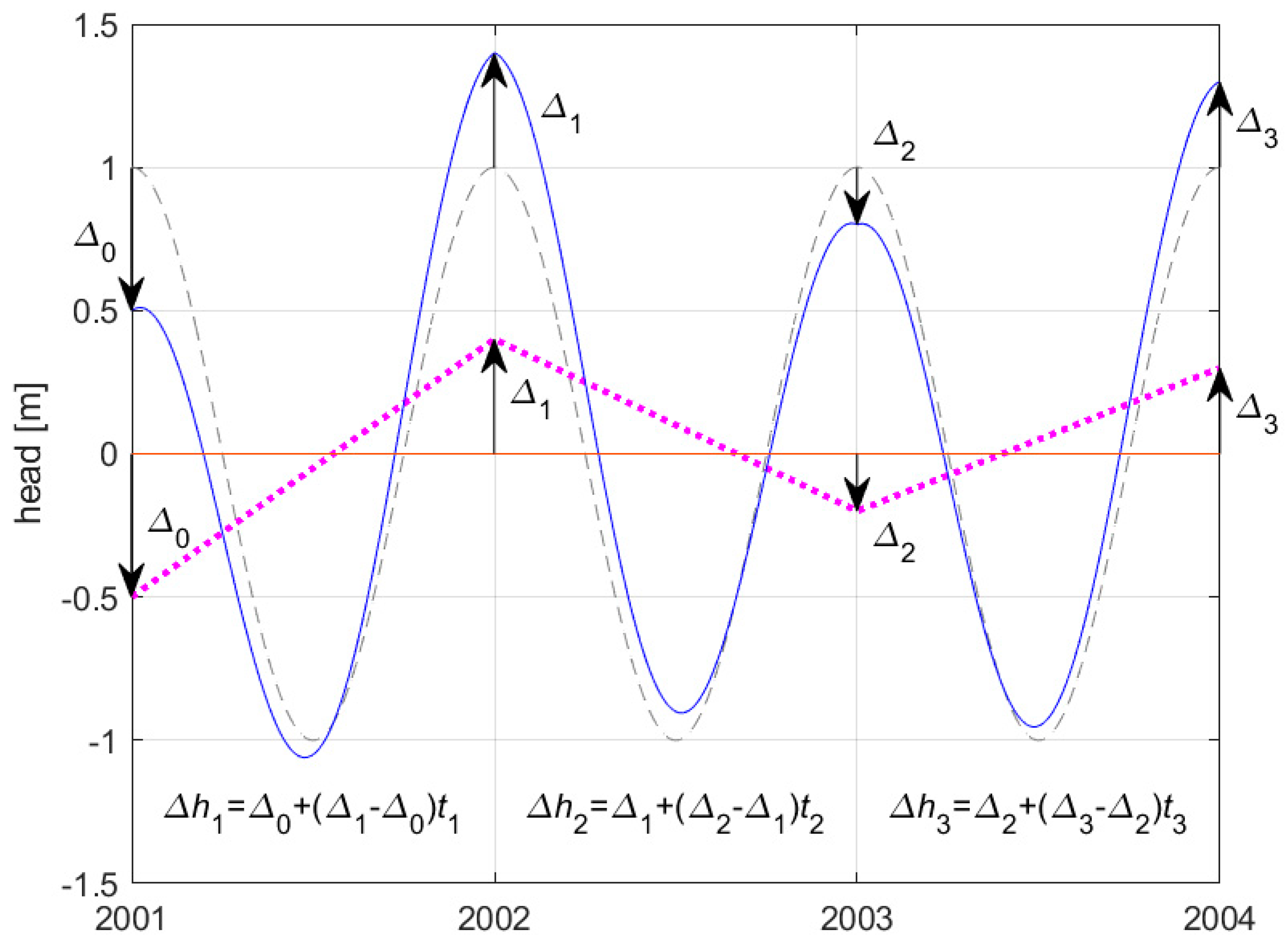
where h2 is groundwater level, h1 is average head (averaged over all data), a is amplitude [m], t is time [d], and τ is phase shift [d]. The amplitude and phase shift are determined by minimizing the sum of the squared error using Matlab’s function fminsearch, which performs multidimensional unconstrained nonlinear minimization using the Nelder-Mead method [35]. A piecewise linear precipitation adjustment was added to account for years with higher or lower precipitation (Figure 3):
where h3 is precipitation-adjusted groundwater level, S is a scale factor, pi is the annual precipitation residual of the current calendar year, pi−1 is the total annual precipitation residual of the previous calendar year, and ti is time [d] in the current year. The precipitation residual is defined as:
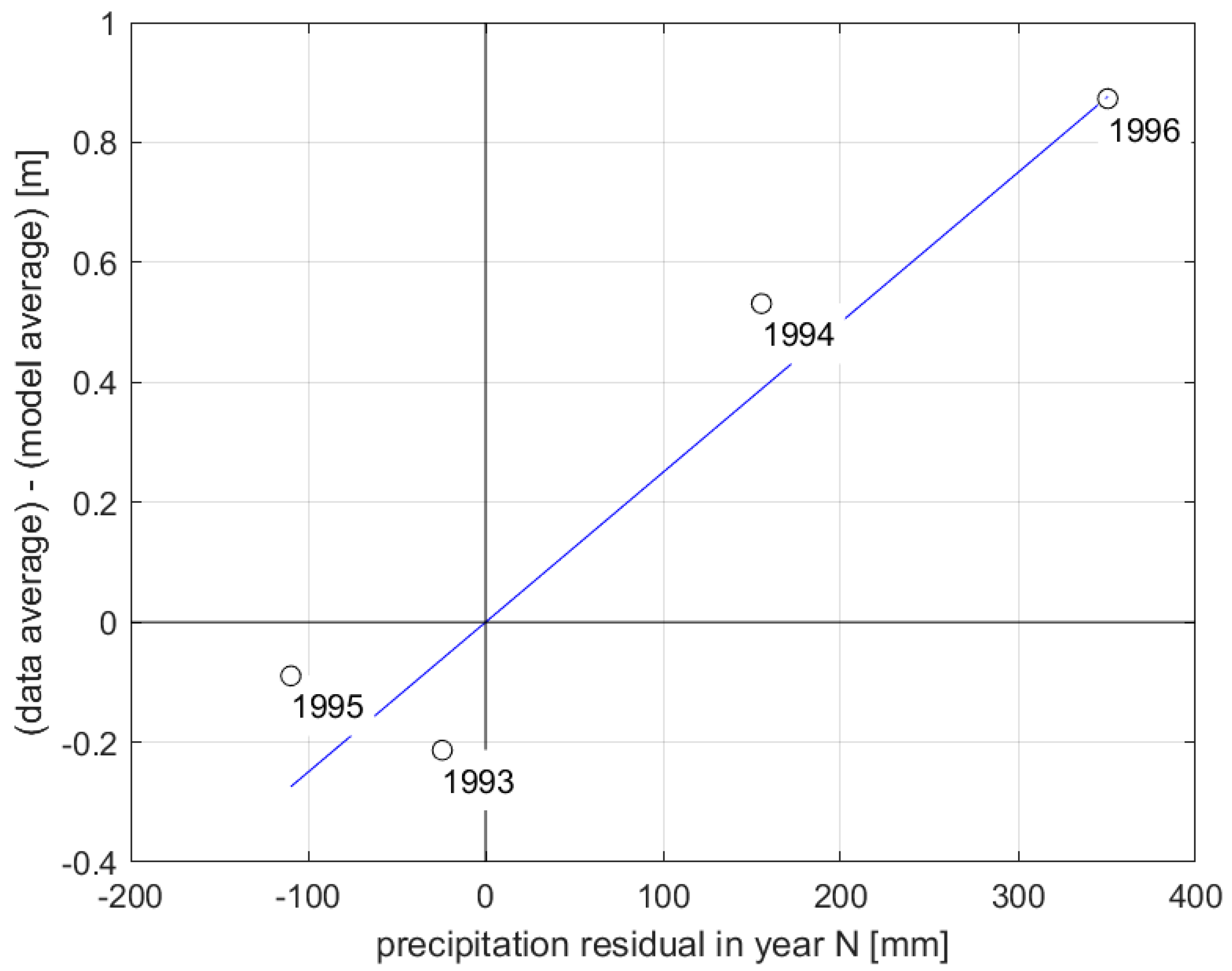
where P is the total annual precipitation and is the mean annual precipitation evaluated over all available data. The scale factor S is the slope of the proportionality
where Δ is groundwater level difference defined as
where hwinter is the measured groundwater level averaged over the first six months of the water year (1 October to 31 March) and h2,winter is the corresponding average of the sinusoidal model in Equation (2). In other words, S is meters of additional winter-averaged groundwater level expected when the annual precipitation is one unit above average. S is determined by minimizing the sum of the squared error using Matlab’s function fminsearch.
Δ = Sp
Δ = hwinter − h2,winter
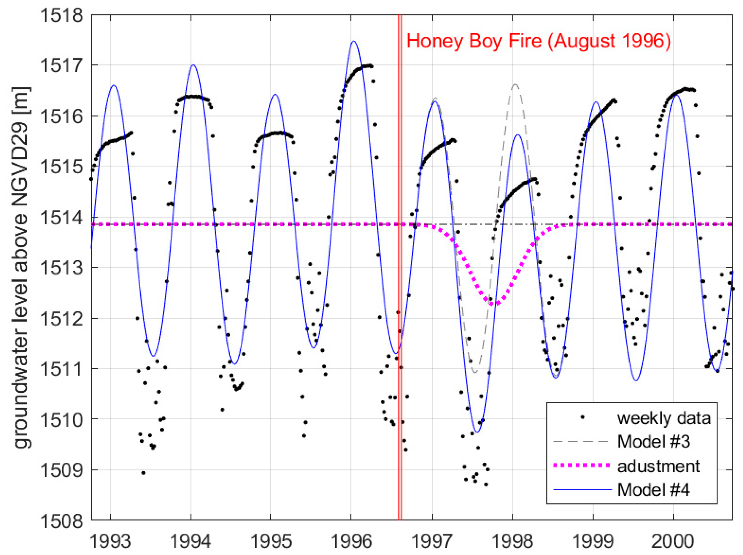
Lacking a quantitative model, the impact of wildfires on groundwater level is modeled empirically as a Gaussian bell curve subtracted from the precipitation-adjusted groundwater level:
where is the scale coefficient of the Gaussian bell curve, is its standard deviation [d], is time [d], and is the time [d] when the Gaussian bell curve reaches its low point. Scale coefficient α, standard deviation σ, and mean time μ are determined by minimizing the sum of the squared error using Matlab’s function fminsearch. This empirical Gaussian bell curve describes how the wildfire affects the groundwater data immediately after the wildfire.
3. Results
The following sections detail the results from queries run in PostGIS and the case study of the Honey Boy Fire.
PostGIS
The spherical distance query (see the Appendix A) identified 331 groundwater wells within the radius (expressed in degrees) corresponding to each wildfire each size class (Table 2). Manual checks were performed on the approximately 20% of these wells with empirical scores w ≥ ½. Only one well met all the search criteria, so given the paucity of the data, it is not possible to accept or reject the hypothesis that wildfires reduce infiltration based on changes in groundwater levels. However, this one site presents a thought-provoking case study that will constitute the remainder of the results.
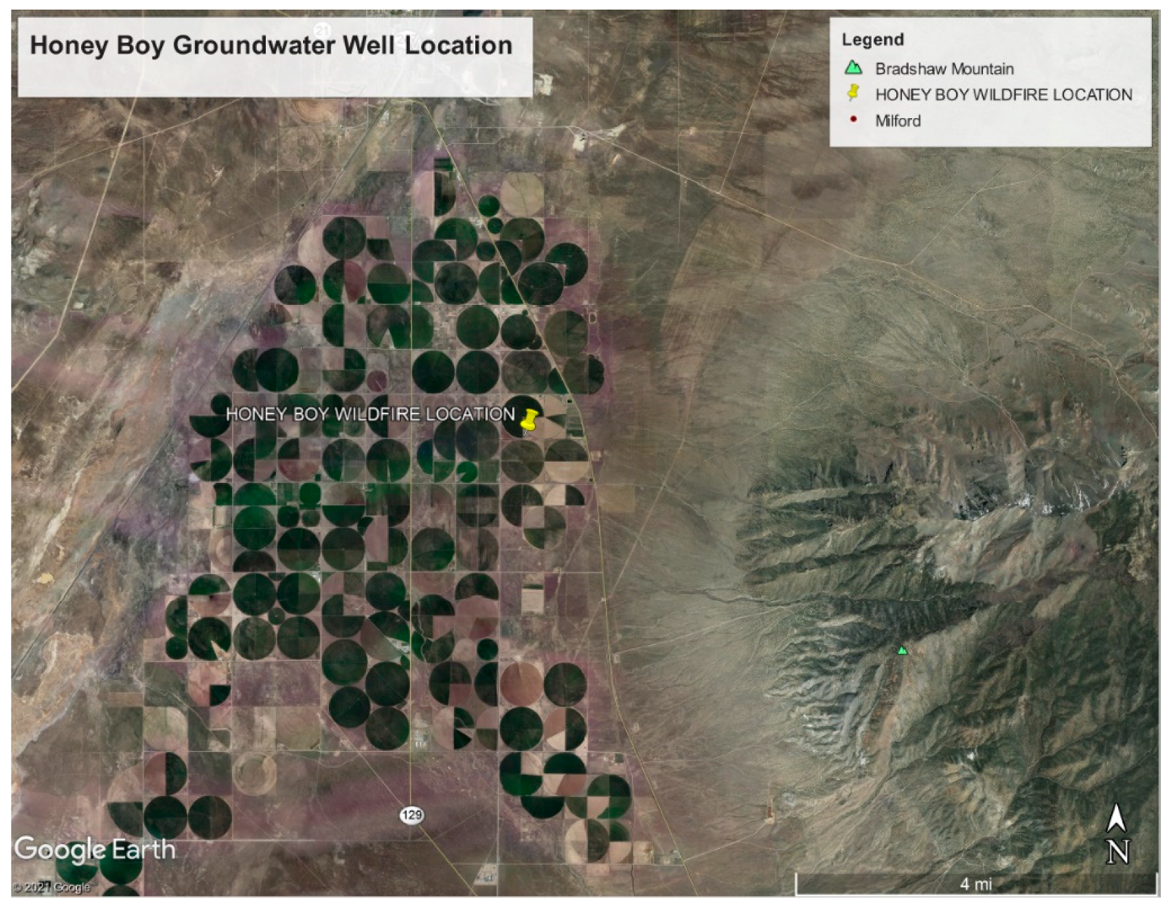
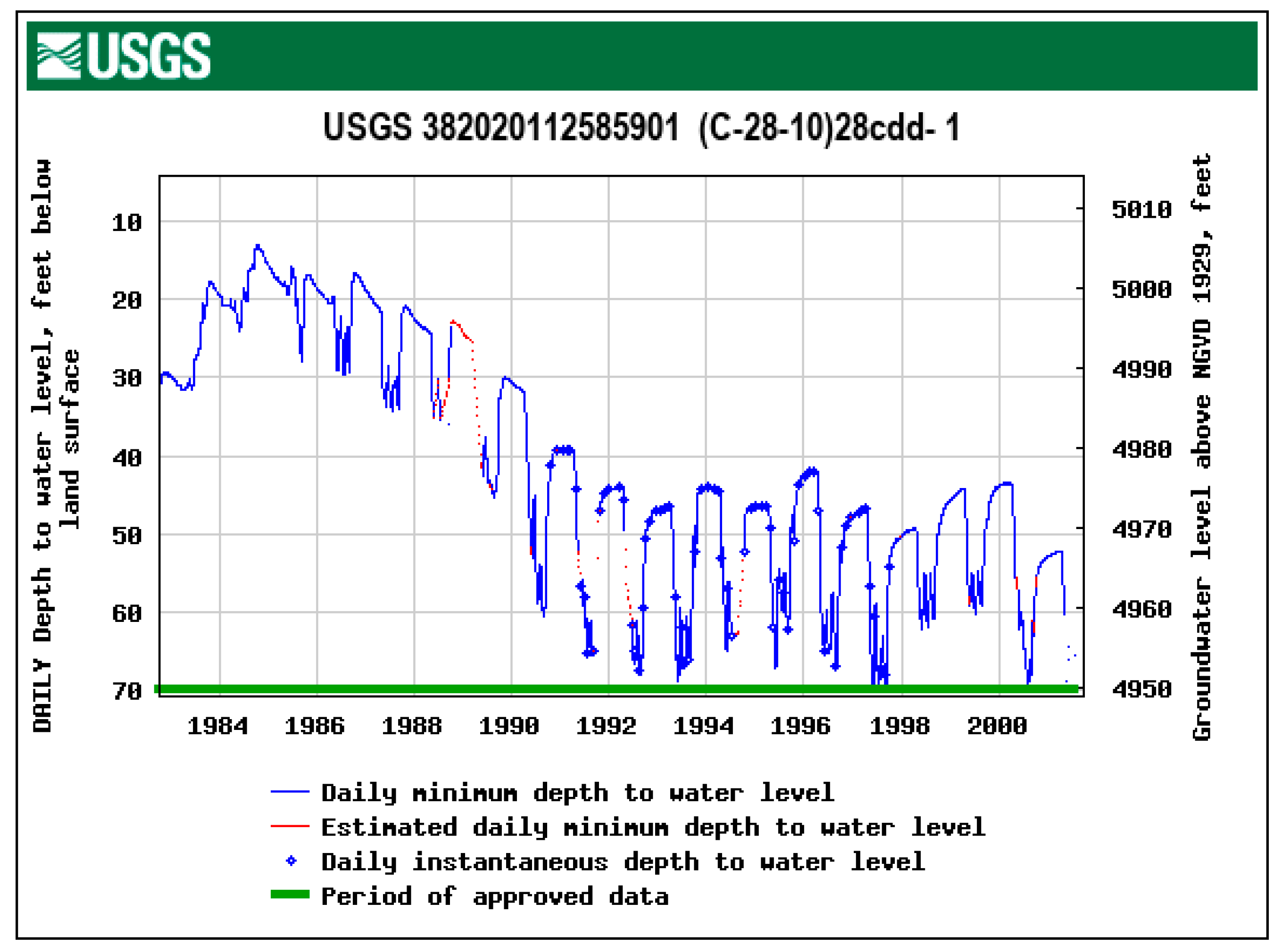
The one groundwater well that met all the search criteria was near the Honey Boy Fire of August 1996 (Figure 4), a 3100 ha (7600 ac) wildfire in Beaver County, Utah, USA [36]. According to data provided by USGS for Site Identification Number 382020112585901, this well has NAD27 coordinates latitude 38°20′20″, longitude 112°58′59″ (converted to NAD83 for the purposes of this study), surface elevation 1529.79 m (5019.00 ft) above NGVD29, hole depth 110 m (360 ft), and well depth 105 m (345 ft). It is located in hydrologic unit 16030007 and completed in the local aquifer designated Valley Fill (100VLFL). This well was located 790 m from the centroid of the Honey Boy Fire, which was a Type G wildfire (assumed equivalent diameter of 3589 m) that burned from 2–15 August 1996. This meant that the well had an empirical weight of w = 0.78, which was within the scoring range considered. Figure 5 shows the entire range of the recorded data measured during the lifetime of this well.
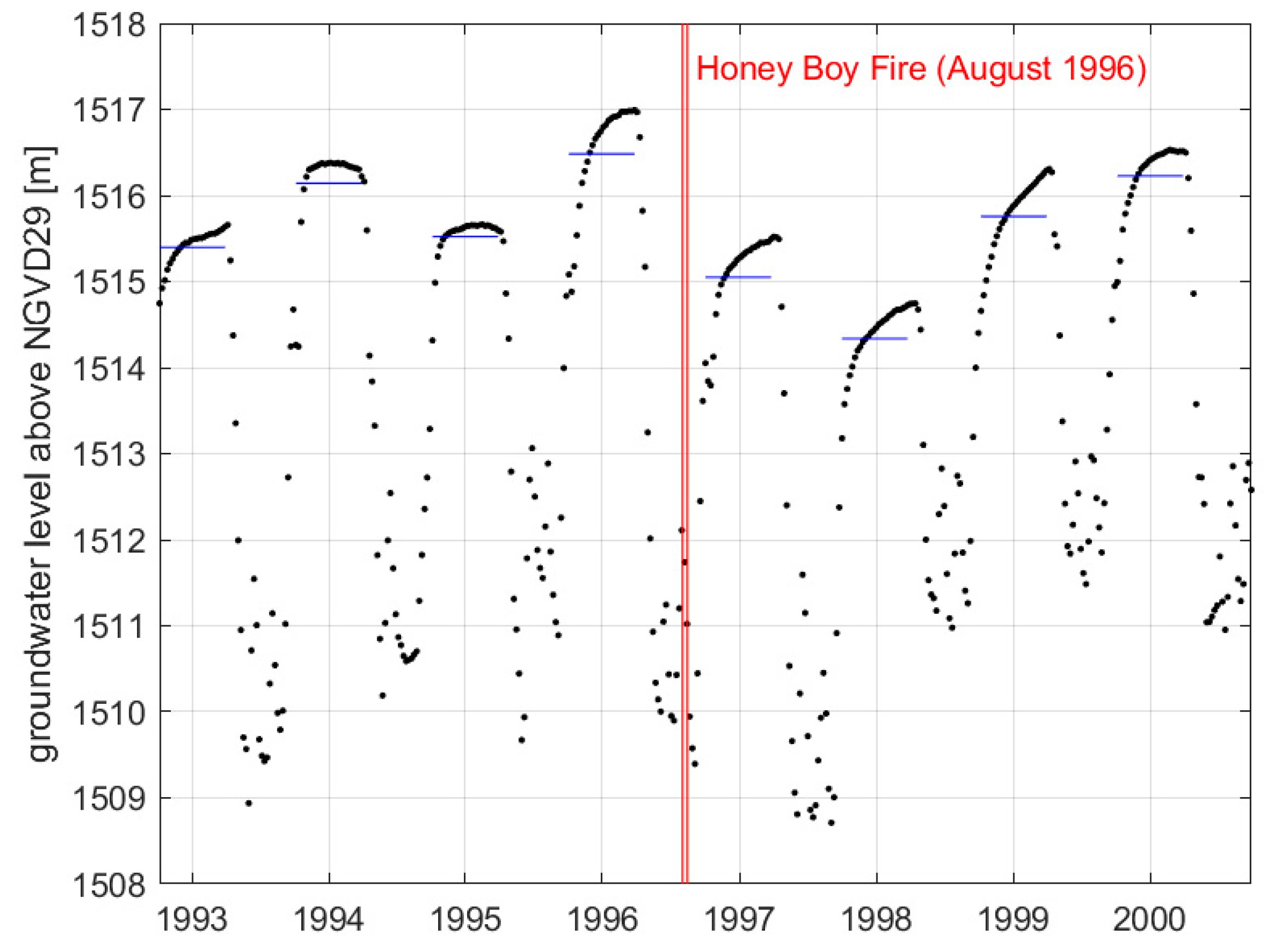
As shown in Figure 5, the weekly-averaged groundwater data for this well have a distinct and predictable periodicity and fluctuate within the desired depth of 30 m from the surface. Although there is a downward trend from 1984 to 1991, the data between 1992 and 2000 stayed within the same elevation range of 1509–1517 m due to controlled irrigation pumping during the summer [37] (pages 84–85). Although these data were influenced by irrigation pumping, they offer consistent measurements over the fall and winter months when there was no irrigation pumping, so accordingly model fitting emphasized the first six months of the water year (1 October to 1 March). Figure 6 shows weekly-averaged groundwater levels converted from feet to meters and focused on the study period comprising the eight water years 1993–2000 (1 October 1992 to 30 September 2000). Figure 6 also shows winter-averaged groundwater levels. Annual precipitation data for water years 1993–2000 were downloaded from the nearest rain gage in Milford, Utah (NOAA station GHCND:USC00425654) and presented in Table 3.
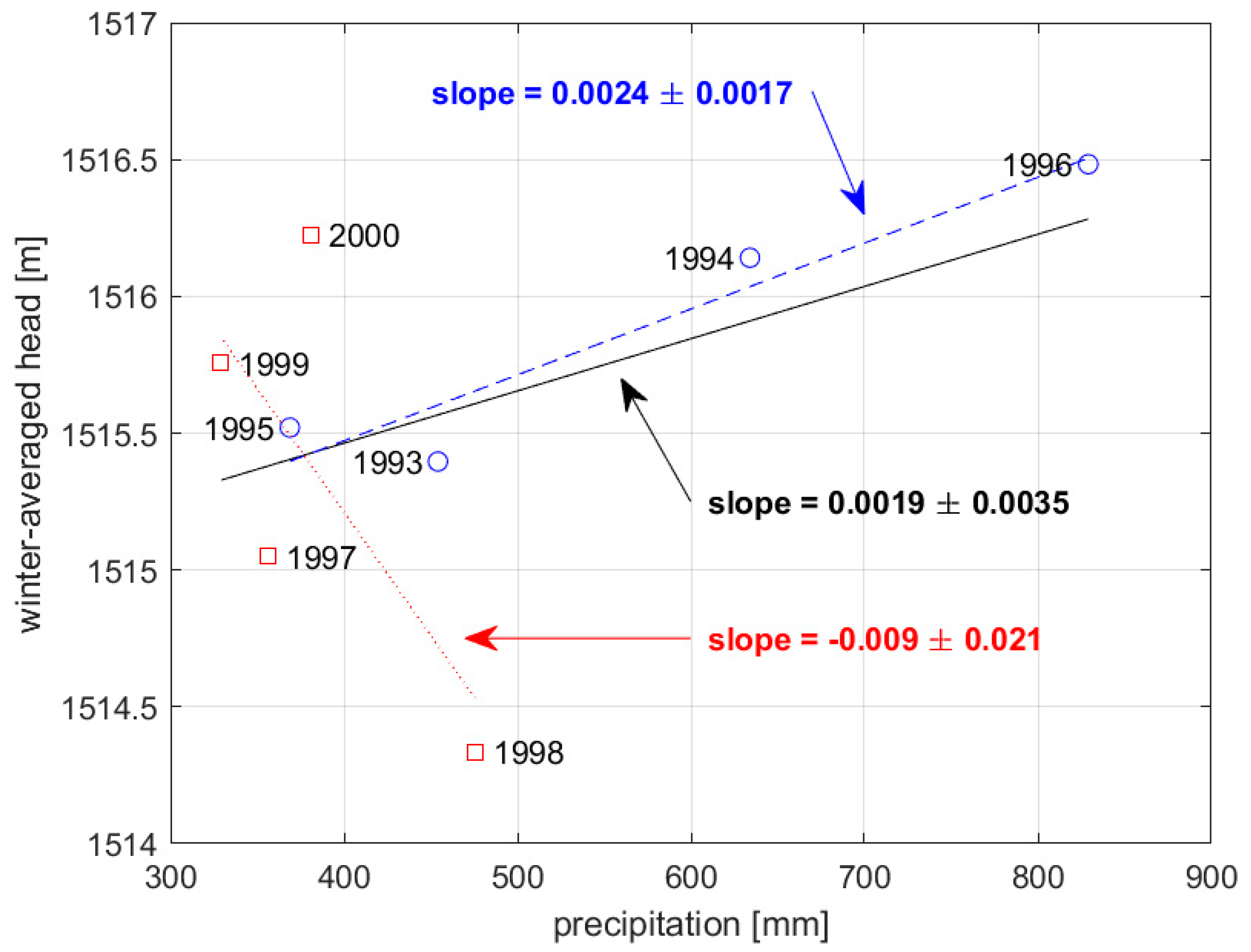
The first of the two methods to analyze these data was to compare the linear regression of groundwater level versus annual precipitation before and after the wildfire (Figure 7). When fitted to all eight water years 1993–2000, shown in black, the slope is not significant (α = 0.05). In the years leading up to the wildfire, shown in blue, there is a significant positive correlation (α = 0.05) between groundwater level and annual precipitation. After the wildfire, shown in red, again the slope is not significant (α = 0.05). Indeed, the post-wildfire data in Figure 7 reveals somewhat erratic fluctuation in groundwater level while the annual precipitation stays relatively consistent between 300–500 mm. This fluctuation suggests that the wildfire may have had an effect on the groundwater recharge of the aquifer.
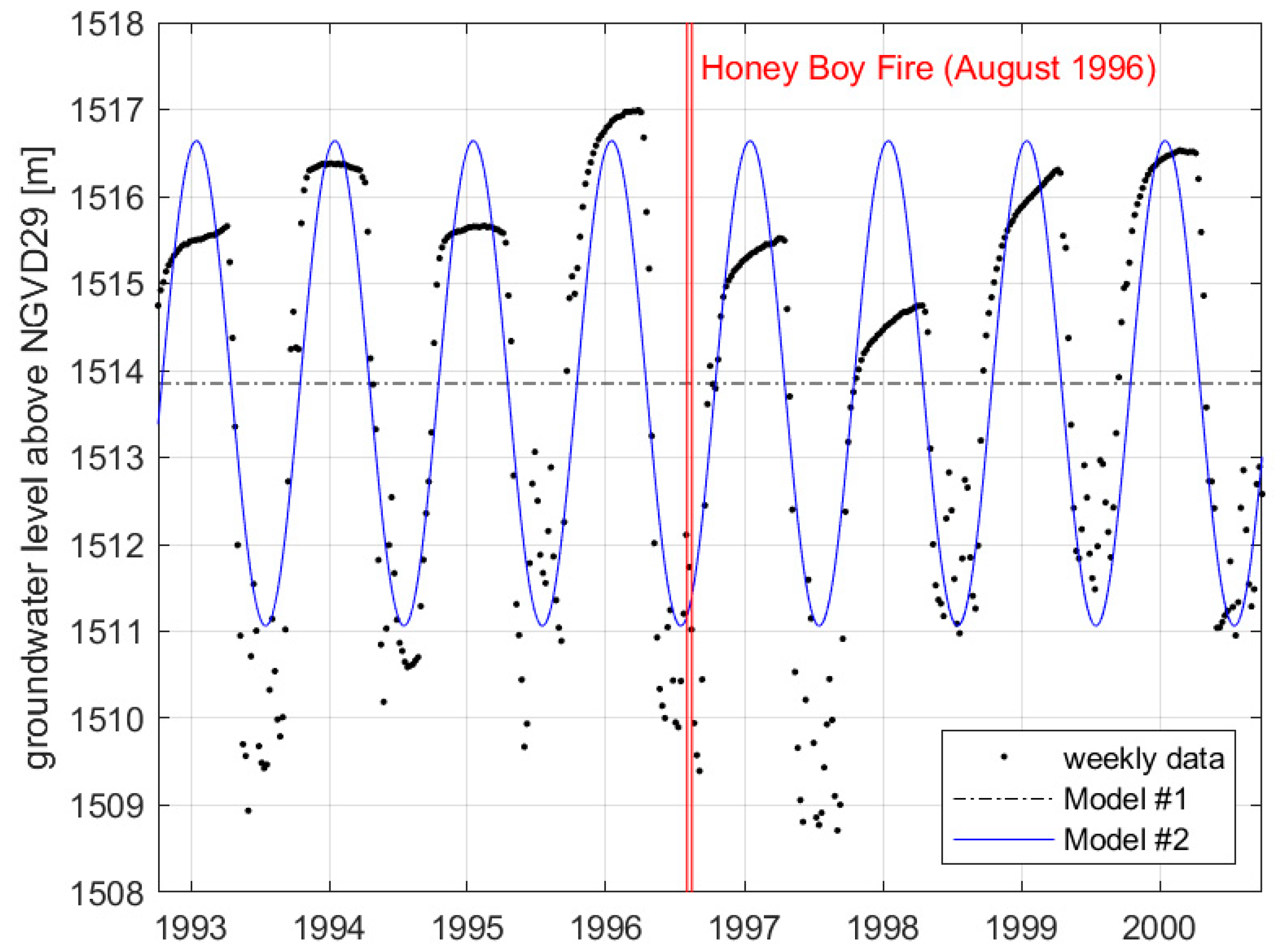
To perform the second method of analysis, the average groundwater level h1 = 1513.85 m was determined by averaging the weekly average data from 1 October 1992 to 30 September 2000. The sinusoidal model, , was found to be:
where t is time [d] where t = 0 is 1 October 1992. This model is shown in Figure 8, indicating an approximation of the groundwater level with a root mean squared error (RMSE) of 1.14 m (Table 4). The precipitation-adjusted model, , is as follows:
where ti is time [d] starting each 1 January, S = 0.0025 m/mm is the scale factor (Figure 9) assuming groundwater levels in (m) and precipitation residuals in [mm] as shown in Table 3. The precipitation-adjusted model is shown in Figure 10, revealing a slightly improved fit to the pre-fire groundwater data, although a slightly worse fit to the full time series (Table 4), suggesting that precipitation cannot explain how the model deviates from regular sinusoidal behavior.
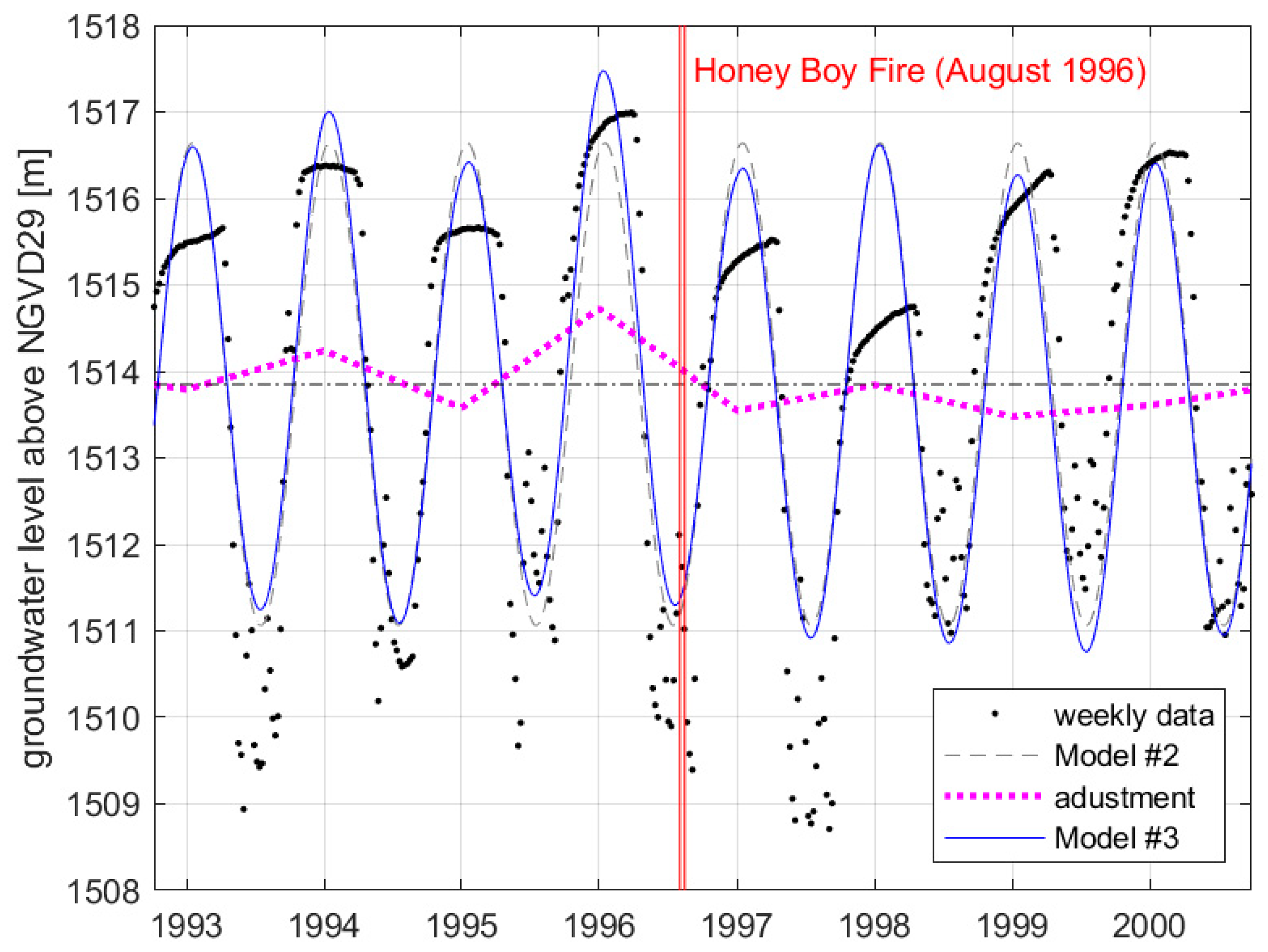
The impact of wildfires on groundwater level is modeled empirically by subtracting a Gaussian bell curve from the model above. The fitted curve is as follows:
where α = 419 is the scale coefficient of the Gaussian bell curve, σ = 106 d is its standard deviation, and μ = 1835 d is the time from the beginning of the groundwater data record to the low point of the Gaussian bell curve (i.e., 434 days or about 14 months after the beginning of the wildfire). The constant before the exponential function is 419/106/(2π)1/2 = 1.58 m, which is the maximum deviation from the precipitation-adjusted sinusoidal model #3. This final model has been plotted in Figure 11, revealing an identical fit to pre-fire groundwater levels and a 6.3% improvement to the full sample period (Table 4).
4. Discussion
The model fitting exercise above offers a new way to parameterize the impact of wildfires on groundwater level, at least in the case of the Honey Boy Fire. The results show a correlation between wildfire and temporarily reduced groundwater levels that may be causal. Let us now revisit three questions from the Introduction: (1) is there a significant change in soil infiltration after a wildfire? (2) Is soil permeability restored to pre-wildfire levels given enough time? (3) What long-term effects may a wildfire have on groundwater?
Regarding the first question, the case study presented here suggests the answer is yes—wildfires do indeed reduce infiltration, consistent with the overwhelming majority of the previous research reviewed in the Introduction. The contribution of the present study was to connect the prior observation of reduced infiltration to a new observation of temporarily reduced groundwater levels. This temporary reduction was modeled by a Gaussian deviation from a precipitation-adjusted sinusoid whose maximum effect came about 14 months after the fire, and whose maximum deviation was about 1.6 m (5.2 ft).
Regarding the second and third questions, the case study presented here suggests that soil permeability is indeed restored to pre-wildfire levels given enough time, so consequently this case study revealed no long-term effects on groundwater. On the contrary, these data have been described by a temporary excursion from a precipitation-adjusted sinusoid. In this particular case study, the maximum effect came about 14 months after the fire, which corresponds to a restoration of pre-fire groundwater levels within about two years. This result is consistent with that of Dymov et al. [19], who reported that most hydrologic effects of wildfire happen in the first 10 years, and with the results of others, who observed fire-related hydrologic effect after two [38], three [14], or five [8,18] years. The conceptual form of the temporary reduction in groundwater level is also consistent with measurements by Ebel [9], whose field site revealed reduced infiltration for all rainfall intensities when measured two years post-fire, but only for high intensity rainfall when measured three years post-fire, and no reduction in infiltration when measured five or seven years post-fire.
This single case study is, of course, not sufficient to confirm or reject the hypothesis that wildfires reduce infiltration based on changes in groundwater levels, which would require analysis of numerous other wildfire-well combinations. Such a study could be undertaken, for example, by considering additional data or by relaxing some of the data selection criteria in this study. For example, one could consider other groundwater wells outside the contiguous United States, or even within it, since there are many more than the 17,754 groundwater wells analyzed here. Another relaxation would be to consider groundwater depths exceeding 30 m, since Pham et al. [29] reported similar wildfire impact on both shallow and deep wells. If more flexible models were available to describe pre-wildfire groundwater fluctuations, it would then be possible to analyze certain groundwater data that could not be described by the precipitation-adjusted sinusoid used here. Additional testing against other data sets, if available, would provide a way to test how generally this model applies to other fires.
Results of this study should also be interpreted in light of the assumptions used in the analysis. Specifically, the effect of precipitation was assumed to depend on annual precipitation for the year ending on 1 February, and the presumed impact on groundwater levels was assumed to be captured by the annual deviation between the winter-averaged measurements and models of groundwater level. This relationship is plausible, and simple enough to be replicated in a future study, but this relationship is certainly not mechanistic. Similarly, the effect of wildfire was parametrized as a Gaussian bell curve, which was chosen as a standard function that offers a temporary excursion from initial and final values of zero. Again, this relationship is certainly not mechanistic.
Having stated these limitations, this method still produced a model that closely followed the groundwater data recorded by USGS, and which offers a straightforward way to parametrize the difference between the groundwater level affected by a wildfire and the predicted groundwater level. It is hoped this method will prove useful, in particular because groundwater levels naturally integrate hydrology over scales larger than wildfires. Accordingly, this method offers one approach to the known complication that wildfire impacts are spatially variable [39]. Having a spatially-integrated method to measure post-fire watershed recovery would also address the known limitation that post-fire mitigation is rarely evaluated at larger scales [4]. It is therefore recommended that additional wells be found and tested using the same approach to determine if the same variations are found in wildfire-affected well data.
5. Conclusions
Analysis of groundwater levels in a wildfire-impacted area are consistent with the hypothesis that wildfires not only increase runoff, but also reduce infiltration to groundwater. For the case study of the Honey Boy Fire, the impact of wildfire was described heuristically by two methods, first by performing linear regression on peak groundwater levels versus annual precipitation to demonstrate a change in their correlation before and the after the wildfire, and second by creating an annual precipitation-adjusted sinusoidal model whose fit was improved by subtracting a Gaussian bell curve describing the temporary reduction in groundwater level after the wildfire. These two methods used to test these effects should be applied for other groundwater wells that are within a wildfire burn radius, and therefore, it is recommended that further studies are pursued under this topic. The effect of wildfires on groundwater is still a significant topic in hydrology; wildfires may have a significant effect not only on soils, runoff, and erosion, but also on infiltration.
Author Contributions
Conceptualization, B.T.J. and D.C.M.; methodology, B.T.J. and D.C.M.; data curation, B.T.J.; writing—original draft preparation, B.T.J.; writing—review and editing, D.C.M. All authors have read and agreed to the published version of the manuscript.
Funding
This research received no external funding.
Acknowledgments
The authors thank Gary Grunwald for suggesting the modeling framework and two anonymous referees whose comments deepened the context and clarified the presentation.
Conflicts of Interest
The authors declare no conflict of interest.
Appendix A
This appendix documents the SQL queries used in PostGIS to identify wildfires with groundwater data, organized under three headings: (1) separating wildfires by size class, (2) synchronizing coordinate systems, and (3) calculating distances between wells and wildfires.
1. Separating wildfires by size class:
Type C Wildfires:
Create table “ThesisV3”.type_c_fire as
Select * From “ThesisV3”.wf_all_1980_2016 where sizeclassn = 3
Type D Wildfires:
Create table “ThesisV3”.type_d_fire as
Select * From “ThesisV3”.wf_all_1980_2016 where sizeclassn = 4
Type E Wildfires:
Create table “ThesisV3”.type_e_fire as
Select * From “ThesisV3”.wf_all_1980_2016 where sizeclassn = 5
Type F Wildfires:
Create table “ThesisV3”.type_f_fire as
Select * From “ThesisV3”.wf_all_1980_2016 where sizeclassn = 6
Type G Wildfires:
Create table “ThesisV3”.type_g_fire as
Select * From “ThesisV3”.wf_all_1980_2016 where sizeclassn = 7
2. Synchronizing coordinate systems:
Select Find_SRID (‘ThesisV3’, ‘type_c_wh_wells’, ‘geom’)
Select UpdateGeometrySRID(‘ThesisV3’, ‘type_c_wh_wells’, ‘geom’, 4269)
3. Calculating distances between wells and wildfires:
Type C Wildfires:
Select c.siteid, a.firename, a.state, a.startdated, a.contrdated,
ST_Distance_Sphere(c.geom, a.geom) As dist_meters_from_well
From “ThesisV3”.”west_wells” AS c INNER JOIN “ThesisV3”.”type_c_fire” As a
ON ST_DWithin(c.geom, a.geom,0.005)
Type D Wildfires:
Select c.siteid, a.firename, a.state, a.startdated, a.contrdated,
ST_Distance_Sphere(c.geom, a.geom) As dist_meters_from_well
From “ThesisV3”.”west_wells” AS c INNER JOIN “ThesisV3”.”type_d_fire” As a
ON ST_DWithin(c.geom, a.geom,0.007)
Type E Wildfires:
Select c.siteid, a.firename, a.state, a.startdated, a.contrdated,
ST_Distance_Sphere(c.geom, a.geom) As dist_meters_from_well
From “ThesisV3”.”west_wells” AS c INNER JOIN “ThesisV3”.”type_e_fire” As a
ON ST_DWithin(c.geom, a.geom,0.011)
Type F Wildfires:
Select c.siteid, a.firename, a.state, a.startdated, a.contrdated,
ST_Distance_Sphere(c.geom, a.geom) As dist_meters_from_well
From “ThesisV3”.”west_wells” AS c INNER JOIN “ThesisV3”.”type_f_fire” As a
ON ST_DWithin(c.geom, a.geom,0.026)
Type G Wildfires:
Select c.siteid, a.firename, a.state, a.startdated, a.contrdated,
ST_Distance_Sphere(c.geom, a.geom) As dist_meters_from_well
From “ThesisV3”.”west_wells” AS c INNER JOIN “ThesisV3”.”type_g_fire” As a
ON ST_DWithin(c.geom, a.geom,0.036)
References
- Ebel, B.A.; Moody, J.A. Rethinking infiltration in wildfire-affected soils. Hydrol. Process. 2013, 27, 1510–1514. [Google Scholar] [CrossRef]
- Gray, M.E.; Zachmann, L.J.; Dickson, B.G. A weekly, continually updated dataset of the probability of large wildfires across western US forests and woodlands. Earth Syst. Sci. Data 2018, 10, 1715–1727. [Google Scholar] [CrossRef] [Green Version]
- Riedel, T.; Weber, T.K.D. Review: The influence of global change on Europe’s water cycle and groundwater recharge. Hydrogeol. J. 2020, 28, 1939–1959. [Google Scholar] [CrossRef]
- Girona-Garcia, A.; Vieira, D.C.S.; Silva, J.; Fernandez, C.; Robichaud, P.R.; Keizer, J.J. Effectiveness of post-fire soil erosion mitigation treatments: A systematic review and meta-analysis. Earth Sci. Rev. 2021, 217, 103611. [Google Scholar] [CrossRef]
- Lopes, A.R.; Girona-Garcia, A.; Corticeiro, S.; Martins, R.; Keizer, J.J.; Vieira, D.C.S. What is wrong with post-fire soil erosion modelling? A meta-analysis on current approaches, research gaps, and future directions. Earth Surf. Process. Landf. 2021, 46, 205–219. [Google Scholar] [CrossRef]
- Tsinnajinnie, L.M.; Frisbee, M.D.; Wilson, J.L. Groundwater from perennial springs provide refuge from wildfire impacts in mountainous semiarid watershed. J. Hydrol. 2021, 596, 125701. [Google Scholar] [CrossRef]
- Lohse, K.; Berhe, A. Soil Signals Tell of Landscape Disturbances. Eos, Transactions, American Geophysical Union. 2020. Available online: https://eos.org/science-updates/soil-signals-tell-of-landscape-disturbances (accessed on 28 October 2020).
- Larson-Nash, S.S.; Robichaud, P.R.; Pierson, F.B.; Moffet, C.A.; Williams, C.J.; Spaeth, K.E.; Brown, R.E.; Lewis, S.A. Recovery of small-scale infiltration and erosion after wildfires. J. Hydrol. Hydromech. 2018, 66, 261–270. [Google Scholar] [CrossRef] [Green Version]
- Ebel, B.A. Temporal evolution of measured and simulated infiltration following wildfire in the Colorado Front Range, USA: Shifting thresholds of runoff generation and hydrologic hazards. J. Hydrol. 2020, 585, 124765. [Google Scholar] [CrossRef]
- Shakesby, R.A.; Doerr, S.H. Wildfire as a hydrological and geomorphological agent. Earth Sci. Rev. 2006, 74, 269–307. [Google Scholar] [CrossRef]
- Cawson, J.G.; Sheridan, G.J.; Smith, H.G.; Lane, P.N.J. Surface runoff and erosion after prescribed burning and the effect of different fire regimes in forests and shrublands: A review. Int. J. Wildland Fire 2012, 21, 857–872. [Google Scholar] [CrossRef]
- Fernandez, C.; Fonturbel, T.; Vega, J.A. Wildfire burned soil organic horizon contribution to runoff and infiltration in a Pinus pinaster forest soil. J. For. Res. 2019, 24, 86–92. [Google Scholar] [CrossRef]
- Balfour, V.N.; Doerr, S.H.; Robichaud, P.R. The temporal evolution of wildfire ash and implications for post-fire infiltration. Int. J. Wildland Fire 2014, 23, 733–745. [Google Scholar] [CrossRef] [Green Version]
- Nyman, P.; Sheridan, G.J.; Smith, H.G.; Lane, P.N.J. Modeling the effects of surface storage, macropore flow and water repellency on infiltration after wildfire. J. Hydrol. 2014, 513, 301–313. [Google Scholar] [CrossRef]
- Ebel, B.A.; Moody, J.A. Synthesis of soil-hydraulic properties and infiltration timescales in wildfire-affected soils. Hydrol. Process. 2017, 31, 324–340. [Google Scholar] [CrossRef]
- Stavi, I. Wildfires in grasslands and shrublands: A review of impacts on vegetation, soil, hydrology, and geomorphology. Water 2019, 11, 1042. [Google Scholar] [CrossRef] [Green Version]
- Malkinson, D.; Wittenberg, L. Post fire induced soil water repellency-Modeling short and long-term processes. Geomorphology 2011, 125, 186–192. [Google Scholar] [CrossRef]
- Robichaud, P.R.; Wagenbrenner, J.W.; Pierson, F.B.; Spaeth, K.E.; Ashmun, L.E.; Moffet, C.A. Infiltration and interrill erosion rates after a wildfire in western Montana, USA. Catena 2016, 142, 77–88. [Google Scholar] [CrossRef] [Green Version]
- Dymov, A.A.; Abakumov, E.V.; Bezkorovaynaya, I.N.; Prokushkin, A.S.; Kuzyakov, Y.V.; Milanovsky, E.Y. Impact of forest fire on soil properties. Theor. Appl. Ecol. 2018, 4, 13–23. [Google Scholar] [CrossRef]
- Certini, G.; Moya, D.; Lucas-Borja, M.E.; Mastrolonardo, G. The impact of fire on soil-dwelling biota: A review. For. Ecol. Manag. 2021, 488, 118989. [Google Scholar] [CrossRef]
- Peterson, C.J. Review of termite forest ecology and opportunities to investigate the relationship of termites to fire. Sociobiology 2010, 56, 313–352. [Google Scholar]
- Mastrorillo, L.; Mazza, R.; Viaroli, S. Recharge process of a dune aquifer (Roman coast, Italy). Acque Sotter. Ital. J. Groundw. 2018, 7, 7–19. [Google Scholar] [CrossRef]
- Giambastiani, B.M.S.; Greggio, N.; Nobili, G.; Dinelli, E.; Antonellini, M. Forest fire effects on groundwater in a coastal aquifer (Ravenna, Italy). Hydrol. Process. 2018, 32, 2377–2389. [Google Scholar] [CrossRef]
- Moody, J.A.; Kinner, D.A.; Úbeda, X. Linking hydraulic properties of fire-affected soils to infiltration and water repellency. J. Hydrol. 2009, 379, 291–303. [Google Scholar] [CrossRef]
- Beatty, S.M.; Smith, J.E. Dynamic soil water repellency and infiltration in post-wildfire soils. Geoderma 2013, 192, 160–172. [Google Scholar] [CrossRef]
- Cawson, J.G.; Nyman, P.; Smith, H.G.; Lane, P.N.J.; Sheridan, G.J. How soil temperatures during prescribed burning affect soil water repellency, infiltration and erosion. Geoderma 2016, 278, 12–22. [Google Scholar] [CrossRef]
- Mansilha, C.; Melo, A.; Martins, Z.E.; Ferreira, I.M.P.L.V.O.; Pereira, A.M.; Marques, J.E. Wildfire effects on groundwater quality from springs connected to small public supply systems in a peri-urban forest area (Braga Region, NW Portugal). Water 2020, 12, 1146. [Google Scholar] [CrossRef] [Green Version]
- Dimitriadou, S.; Katsanou, K.; Charalabopoulos, S.; Lambrakis, N. Interpretation of the Factors Defining Groundwater Quality of the Site Subjected to the Wildfire of 2007 in Ilia Prefecture, South-Western Greece. Geosciences 2018, 8, 108. [Google Scholar] [CrossRef] [Green Version]
- Pham, H.V.; Le, P.; Berli, M. A data-driven approach to quantifying the correlation between groundwater and wildfire in the United States. In Proceedings of the American Geophysical Union Fall Meeting, Online, 1–17 December 2020; p. H087-0025. [Google Scholar]
- Schneider, K.E.; Rust, A.J.; Randall, J.; Hogue, T.S. Modelling post-fire hydrologic recovery in snow dominated catchments in Colorado’s San Juan Mountains. In Proceedings of the American Geophysical Union Fall Meeting, Online, 1–17 December 2020; p. H095-06. [Google Scholar]
- ArcGIS. US Wildfires 1980–2016. Available online: https://hub.arcgis.com/datasets/tga::us-wildfires-1980-2016 (accessed on 21 April 2021).
- U.S. Geological Survey. Active Groundwater Level Network. Available online: https://groundwaterwatch.usgs.gov/default.asp (accessed on 21 April 2021).
- National Wildfire Coordinating Group. Size Class of Fire. Available online: https://www.nwcg.gov/term/glossary/size-class-of-fire (accessed on 1 November 2020).
- Belsley, D.A.; Kuh, E.; Welsch, R.E. Regression Diagnostics; John Wiley and Sons, Inc.: Hoboken, NJ, USA, 1980. [Google Scholar]
- Lagarias, J.C.; Reeds, J.A.; Wright, M.H.; Wright, P.E. Convergence properties of the Nelder-Mead simplex method in low dimensions. SIAM J. Optim. 1998, 9, 112–147. [Google Scholar] [CrossRef] [Green Version]
- Swensen, J.; Romboy, D. Utah is Nation’s Hot Spot for Wildfires. Deseret News. 6 August 1996. Available online: https://www.deseret.com/1996/8/6/19258572/utah-is-nation-s-hot-spot-for-wildfires (accessed on 21 April 2021).
- Burden, C.B. Ground-Water Conditions in Utah; Report No. 42; Division of Water Resources, Utah Department of Natural Resources: Salt Lake City, UT, USA, 2001.
- Williams, C.J.; Pierson, F.B.; Al-Hamdan, O.Z.; Kormos, P.R.; Hardegree, S.P.; Clark, P.E. Can wildfire serve as an ecohydrologic threshold- reversal mechanism on juniper-encroached shrublands? Ecohydrology 2014, 7, 453–477. [Google Scholar] [CrossRef]
- Goldshleger, N.; Ben-Dor, E.; Lugassi, R.; Eshel, G. Soil degradation monitoring by remote sensing: Examples with three degradation processes. Soil Sci. Soc. Am. J. 2010, 74, 1433–1445. [Google Scholar] [CrossRef]
Figure 1.
Wildfire locations (1980 through 2016) within the United States.

Figure 2.
USGS well locations within the United States.

Figure 3.
Schematic of the precipitation adjustment Δh in Equation (3).

Figure 4.
Location of the USGS groundwater well in Beaver County, Utah. Note its location within farmland area.
Figure 4.
Location of the USGS groundwater well in Beaver County, Utah. Note its location within farmland area.

Figure 5.
The daily groundwater level for USGS well 382020112585901 measured over the lifetime of this groundwater well from 1983 to 2001. This well was 790 m from the centroid of the Honey Boy Fire of August 1996.
Figure 5.
The daily groundwater level for USGS well 382020112585901 measured over the lifetime of this groundwater well from 1983 to 2001. This well was 790 m from the centroid of the Honey Boy Fire of August 1996.

Figure 6.
Weekly-averaged groundwater level in USGS well 382020112585901 for the study period of 1 October 1992 through 30 September 2000. The horizontal blue lines are groundwater levels averaged each winter from 1 October through 31 March.
Figure 6.
Weekly-averaged groundwater level in USGS well 382020112585901 for the study period of 1 October 1992 through 30 September 2000. The horizontal blue lines are groundwater levels averaged each winter from 1 October through 31 March.

Figure 7.
Winter-averaged groundwater level versus annual precipitation each 1 February. The correlation for all eight years (1993–2000) is a black solid line; the correlation for pre-wildfire years (1993–1996) is a blue dashed line; the correlation for post-wildfire years (1996–2000) is a red dotted line. Each slope is reported as a 95% confidence interval using the t-test with 7 degrees of freedom when n = 8 and with 3 degrees of freedom when n = 4. Only the pre-fire correlation is significant.

Figure 8.
Sinusoidal model #2 (in blue) fits much better than constant model #1, reducing the root mean squared error (RMSE) by 50% for the study period from 1993–2000 and by 55% for the pre-fire years of 1993–1996 (Table 4).
Figure 8.
Sinusoidal model #2 (in blue) fits much better than constant model #1, reducing the root mean squared error (RMSE) by 50% for the study period from 1993–2000 and by 55% for the pre-fire years of 1993–1996 (Table 4).

Figure 9.
Proportionality between winter-averaged groundwater residual Δ and precipitation residual p, modeled as Δ = Sp, where the slope S = 0.0025 m/mm.
Figure 9.
Proportionality between winter-averaged groundwater residual Δ and precipitation residual p, modeled as Δ = Sp, where the slope S = 0.0025 m/mm.

Figure 10.
Precipitation-adjusted model #3 (in blue) provides only a modest improvement of 4.3% to the pre-fire RMSE, and a slight degradation of 0.9% to the RMSE for the entire study period.
Figure 10.
Precipitation-adjusted model #3 (in blue) provides only a modest improvement of 4.3% to the pre-fire RMSE, and a slight degradation of 0.9% to the RMSE for the entire study period.

Figure 11.
Fire-adjusted model #4 does not change the RMSE for the pre-fire period but provides a 6.3% improvement for the post-fire period (Table 4). The impact of the Honey Boy Fire is modeled as a Gaussian deviation from the precipitation-adjusted model #3, where the Gaussian deviation is centered 434 days after the beginning of the fire, with a standard deviation of 106 days, and a maximum groundwater level depression of 1.58 m.


Table 1.
Wildfire areas by type with equivalent radii in degrees. Measurements assume the coordinate system is either the North American Datum of 1983 or the World Geodetic System of 1984 [33].
Table 1.
Wildfire areas by type with equivalent radii in degrees. Measurements assume the coordinate system is either the North American Datum of 1983 or the World Geodetic System of 1984 [33].
| Wildfire Type | Maximum Area (ac) | Maximum Area (ha) | Assumed Radius (°) |
|---|---|---|---|
| C | 100 | 40 | 0.005 |
| D | 300 | 120 | 0.007 |
| E | 1000 | 400 | 0.011 |
| F | 5000 | 2000 | 0.026 |
| G | none | none | 0.036 |
Table 2.
The number of results found using PostGIS.
| Wildfire Class | Number of Groundwater Wells within the Approximated Burn Radius | Number of Groundwater Wells with a Theoretical Score Higher Than 0.5 |
|---|---|---|
| Type C Wildfires | 22 | 5 |
| Type D Wildfires | 5 | 1 |
| Type E Wildfires | 25 | 4 |
| Type F Wildfires | 136 | 30 |
| Type G Wildfires | 143 | 25 |
| Totals | 331 | 65 |
Table 3.
The annual precipitation recorded by NOAA in Cedar City, Utah, USA ending 1 February 1993 to 2000.
Table 3.
The annual precipitation recorded by NOAA in Cedar City, Utah, USA ending 1 February 1993 to 2000.
| Chart Date | Annual Precipitation (ft) | Annual Precipitation (mm) | Precipitation Residual (mm) |
|---|---|---|---|
| 2 January 1993 | 1.49 | 454 | −14 |
| 2 January 1994 | 2.08 | 634 | 166 |
| 2 January 1995 | 1.21 | 369 | −100 |
| 2 January 1996 | 2.72 | 829 | 361 |
| 2 January 1997 | 1.17 | 357 | −112 |
| 2 January 1998 | 1.56 | 475 | 7 |
| 2 January 1999 | 1.08 | 329 | −139 |
| 2 January 2000 | 1.25 | 381 | −87 |
Table 4.
Root mean squared error (RMSE) for each of the four models.
| Pre-Fire | All Dates | |||
|---|---|---|---|---|
| Model | RMSE | Improvement | RMSE | Improvement |
| 1—average | 1.67 | - | 2.28 | - |
| 2—sinusoid | 0.76 | 55% | 1.14 | 50% |
| 3—precipitation adjusted | 0.72 | 4.3% | 1.15 | −0.9% |
| 4—fire adjusted | 0.72 | 0.0% | 1.08 | 6.3% |
Publisher’s Note: MDPI stays neutral with regard to jurisdictional claims in published maps and institutional affiliations. |
© 2021 by the authors. Licensee MDPI, Basel, Switzerland. This article is an open access article distributed under the terms and conditions of the Creative Commons Attribution (CC BY) license (https://creativecommons.org/licenses/by/4.0/).
Share and Cite
MDPI and ACS Style
Johnk, B.T.; Mays, D.C. Wildfire Impacts on Groundwater Aquifers: A Case Study of the 1996 Honey Boy Fire in Beaver County, Utah, USA. Water 2021, 13, 2279. https://doi.org/10.3390/w13162279
AMA Style
Johnk BT, Mays DC. Wildfire Impacts on Groundwater Aquifers: A Case Study of the 1996 Honey Boy Fire in Beaver County, Utah, USA. Water. 2021; 13(16):2279. https://doi.org/10.3390/w13162279
Chicago/Turabian StyleJohnk, Benjamin T., and David C. Mays. 2021. "Wildfire Impacts on Groundwater Aquifers: A Case Study of the 1996 Honey Boy Fire in Beaver County, Utah, USA" Water 13, no. 16: 2279. https://doi.org/10.3390/w13162279
Note that from the first issue of 2016, this journal uses article numbers instead of page numbers. See further details here.