
Cloud Physical and Climatological Factors for the Determination of Rain Intensity

Ombros, Kvillingevägen 6, SE-616 34 Åby, Sweden
Water 2021, 13(16), 2292; https://doi.org/10.3390/w13162292
Submission received: 2 July 2021
/
Revised: 13 August 2021
/
Accepted: 17 August 2021
/
Published: 21 August 2021
(This article belongs to the Special Issue Extreme Value Analysis of Short-Duration Rainfall and Intensity–Duration–Frequency Models)
Abstract
:The focus of this research is to develop a general method for estimation of rain intensity for application in various geographical regions. In a world with a changing climate, a high importance is attributed to the potential threats caused by increased temperature and rainfall intensity levels. The rainfall intensity climate is here interpreted by a combination of cloud physical factors affecting rain intensity and further developed by the use of climate data and rain intensity statistics. A formula was developed that estimates extreme rainfall and the frequency of these extremes with durations in the intervals of 5 min to 24 h. The obtained estimates are compared in this article with results from statistical methods for the extreme value analysis of measurements. The comparison shows about 90% of the explained variance. The coefficients in the formula are connected with climatological predictors based on the climatological norms of temperature and rainfall. Rain intensity maps over Sweden were produced using the developed formula. Examples of the function of the formula are also given for six European countries. The application of the formula in connection with the probable maximum precipitation (PMP) is presented, where the return period of extreme rainfall is a key factor. The formula is tested with an assumed increased warming of the atmosphere of 1 to 5 °C, and the result indicates an increase of 5.9% of the rainfall amount per each warming degree in intense rainfall.
1. Introduction
The background of this study is that extreme cloudburst events affect a multitude of society’s fundamental infrastructures. The urban sector is particularly sensitive, where flooding and erosion can cause substantial human and economic damages [1].
Due to global warming, precipitation extremes are expected to be more intense [2] and cause large social and economic losses [3].
Our knowledge of intensity–duration–frequency (IDF) models of rainfall is today generally built on a variety of methods for extreme value analysis (EVA). EVA methods are generally based on theories that use rainfall intensity measurements as the input. Among the methods in use is the generalized extreme value (GEV) distribution [4,5]. GEV is developed within extreme value theory and combines the Gumbel [6], Fréchet [7] and Weibull [8] families, also known as type I, II and III extreme value distributions, respectively. The extreme value methods are designed to handle extreme values and these extreme values are often based on statistical analysis of so-called ‘block rains’ (see Section Block Rains below).
In Sweden, the regional statistics were developed in 1979 [9] by use of a factor that consisted of the difference between the average summer temperature and the mean temperature during a month in spring. This factor was created to emphasize convective rainfall and reduce the influence of low-intensity rainfall caused by oreigenic rainfall [10,11]. When convection also started to be more intense in spring, this approach had to be abandoned and a new method was introduced [12]. This method was based on some cloud physics and calibrated with EVA data and is recommended in today’s guidelines [13] in Sweden. The cloud physics approach was further developed and applied to climatological data for Europe [14].
Our knowledge of the nature and characteristics of rainfall intensity is based on numerous studies, but nevertheless, the gaps in our knowledge are still unsatisfactory. Whilst EVA methods can provide good estimates of IDF in locations for which detailed historical data are available, the estimates have restricted applicability both for predicting future IDF models in a changing climate, and for predicting IDF models at other locations for which such data are not available.
The objective of the present investigation is to develop an alternative and improved method for estimating IDF statistics based on cloud physical considerations with further development involving climatological predictors. The work aims at improving and facilitating the estimation of rainfall intensity for locations in various climatological regions. Improvements regarding the estimation of the probable maximum precipitation and the estimation of what the effect a warming world will have on the level of rain intensity are items that are also approached in this study. The main objective is thus to develop a formula for intense rainfall with intensity levels, durations and frequency of occurrence with applicability to various climatological regions, or ideally with global applicability.
The developed formula, R, is offered as a new tool for responding to problems related to the design of urban water discharge structures and to address the issue regarding the future level of rain intensity in a changing climate. The coefficients in the formula are connected with climatological predictors and are therefore relatively unchanged when the climate changes. The formula was tested with data from countries in Europe and also partly with data from Asia.
Block Rains
Block rains (see an example in Figure 1) describe mean rainfall intensities over fixed duration periods (5 min, 10 min …). These block rains are generated from time series of rain intensity measurements [15]. Successive time windows of selected durations (5 min, 10 min …) pass through the series of data and the level of rain intensity is stored as block rains for the respective duration. The block rains are then ranked in size, and the frequency of the extremes then form a basis for treatment by EVA methods.
Figure 1 illustrates how a block rain (shown in blue) in the scanning of a data series is centered at the maximum of a rain shower before continuing to sweep over all parts of the data series.
2. Materials and Methods
2.1. Data
Information on rainfall and associated meteorological parameters were collected and organized for the development of a mathematical expression with a focus on rain intensity. To overcome the problem of a lack of high-resolution rainfall intensity data, a request of statistics on rain intensity data was sent at the beginning of this project to 26 director generals of west European weather services. The response was positive at most weather services and at least some data were sent. Some weather services did not respond or did not send useful data. It should be noted that data stocks with rain intensity data with a resolution of 5 min or better are often collected by other initiatives than the meteorological services; local authorities that are involved with urban sewer planning and design are frequently building and operating local rain data collections.
This work was preceded by a first approach with a cloud physical view [12]. Data on extreme values of rain intensity were retrieved from European weather services. Climatological data from the E-OBS gridded dataset over Europe were also extracted. The type of gridded data that were extracted concerned the 0.22-degree rotated grid [16]. This E-OBS dataset was used to evaluate the normal values of rainfall and temperature at the rain intensity stations that were obtained.
The retrieved European data stock was too limited for a more general development of an intensity–duration–frequency relationship with the potential for global applications.
Consequently, the European data were supplemented with a small part of the data from a study containing Asian and Australian locations [17]. In that way, extremely abundant rainfall from Asian monsoon locations was also included as well as extremely low rainfall from the desert-like interior of Australia.
A problem that emerged during the data phase was that the collected stock of data was not homogeneous: countries operated various rain instruments with different error properties and also had various routines for their estimation of IDF statistics. The processing of meteorological data to obtain climatological norms also differed between individual countries. Take the following as an example: With Australian data, no daily mean values of climate data were easily available. Instead, monthly temperature values were roughly estimated by use of the arithmetic average of the monthly minimum value and the monthly maximum value, an unsatisfactory solution. With limited research resources available, it was decided to use the available raw, but not fully homogenous, data.
The locations with rain intensity data (5 min or better resolution) were generally not situated where official meteorological stations were situated. This fact meant that it was not easy to access climate norms for the rain intensity locations. To overcome the problem of retrieving climate norms for stations with rain intensity data, it was decided to interpolate from the E-OBS gridded data for these places. The primary aim was to get the normal monthly temperature and rainfall data for the summer months June–August, as these months generally are the months with intense convection. For stations in Asia, however, it was not possible to stick to this “summer rule” due to the monsoon climate. See Section 2.2.2 items 1–3 for the procedures on how to handle these data.
Various models for the estimation of IDF statistics with climate data as predictors were tested with locations where rain intensity statistics were available. The outcome from these testing activities was that the best predictors consisted of 30-year normal values of the sum of measured rainfall during the two heaviest rain months and the average of 30-year normal temperature values during these two months. The normal yearly sum of precipitation also turned out to be important. The various models used for testing were evaluated foremost by the results on the magnitude of the explained variance between the model and the rain intensity data.
Other factors including the height above sea level, a type of thunder index representing the stability of air layers and several other potential predictors, like monthly frequency of rainfall extremes, turned out not to be as successful as the climatological variables mentioned above. A report in Swedish has been published on these variables [14].
For an IDF formula to be applicable in various climatological regions, it is important to consider how rainfall and temperature data are collected and processed. A multitude of error sources exists and will influence the geographical/climatological interpretation of IDF results. Some of the problems with the quality of rainfall intensity data are as follows:
- National types of instruments with different error types. There are weighing instruments, tipping buckets, drop-counting devices and laser-based instruments (distrometers), among others.
- Various national strategies are applied for the choice of the site of the instruments in relation to surrounding buildings/vegetation. It is particularly difficult to place instruments in urban areas due to sheltering and wind tunnel effects from surrounding buildings [18].
- Differences in the methods for the allocation of rains in blocks (during 5 min, 10 min …) and for the coupling of the block rains to the return period [22].
- The type of method of extreme value analysis results in different estimates of the return period of block rains.
- Grid-based values of climatological variables, in this study gridded data (“E-obs data”) over parts of Europe [16], have been used to estimate climate norms at locations with rain intensity data. This means that some data are smoothed over a region and other data concern specific geographical locations.
The total data were randomly divided into sets (Supplementary Materials) R1 and R2 for cross validation. This procedure resulted in dataset R1, with 4132 intensity values from 70 stations. The dataset R2 contained 4306 intensity values from 78 stations. A certain inhomogeneity exists in datasets R1 and R2, in that the European data consisted of summer months, whilst data for a few extracted stations in Asia/Australia were selected for the two rainiest months.
The development of the IDF equation was concentrated on the data contained in dataset R1. Dataset R2 was mainly used for verification/applications with the developed relationship.
2.2. Development of an Expression Related to Intense Rainfall
An extreme rainfall formula, “R”, for rainfall intensity was developed and is described in the next two subsections.
2.2.1. First Approach Based on Cloud Physics
The basic approach was to develop an expression that contains the main physical factors connected with intense rain, which are of key importance for the interpretation of the rainfall intensity, duration and frequency of rainfall events. The rainfall intensity climate on our earth is interpreted by a combination of these cloud factors, climatological norms and rain intensity statistics of the EVA type.
A unit depth of air with height Δz is considered. With r as the mixing ratio and as the density of dry air, the total water vapor content is [23]: where storage of water in clouds is disregarded, as the total accumulated water in the column is the focus. The condensation rate then becomes the same as the rainfall intensity (a pseudo adiabatic assumption).
If R’ denotes the rain intensity in the studied atmospheric layer, then as : . The vertical velocity within the layer is expressed as and if we ignore the change of the thickness of the layer, the above expression can be expressed as: .
Let be the partial pressure of the water vapor and be the total air pressure. As the ratio of the gas constant of water vapor to that of dry air is 0.622 [23] then the mixing ratio can be expressed as and, consequently: .
Simplification gives approximately: .
With the equation of the state for dry air: , where is the air temperature and is the gas constant for dry air, the following expression is obtained: .
The water vapor terms (where ‘’ is contained) are determined for saturated conditions by temperature and pressure. The rain intensity can thus be determined if the thickness of the atmospheric layer and the vertical velocity are known. Integration of the above equation for the saturated vertical atmospheric layer gives us the simplification:
where R’ is the rain intensity that is formed in the atmospheric layer with height ΔH and λ represents a mean value of the water vapor terms effect in the layer. Let denote the temperature excess in the studied atmospheric layer relative to the temperature in the environment. According to the parcel method for convection, the kinetic energy for a depth of saturated air that is raised from a level to a level can be expressed as: .
From this equation it follows that is proportional to . The equation for can then be expressed as:
where represents the average value of the difference in temperature between the air parcel and the temperature in the surrounding air for the vertical atmospheric layer.
Equation (2) gives the rain intensity as a function of the buoyancy given by the temperature difference between the air parcel and the surrounding air in the vertical column and the vertical magnitude of the cloud. Dry air that is mixed with the cloud will retard the convective development and has to be included in the formula as an entrainment factor.
IDF statistics contain very limited information about physical factors affecting rain intensity connected with individual rain showers. The intense rainfall in the core of a raining unit will decrease with distance from its center. The spatial distance is here simplified by using the block rain time of the rainfall, making it possible to formulate an expression of entrainment. A simple factor, , for the reduction of the convection is suggested: , where = constant (scale factor), = rain duration (block rain, see below)distance from the centre of intense rainfall and = exponent that regulates the reduction from the maximum level of the rain.
The available information is based on statistics of measured data on the intensity, duration and frequency of rain. Equation (2) with entrainment included then becomes:
To generate IDF statistics, the most intense parts of the rainfall events were selected. For the respective rain events, the amount of rain during specified duration intervals (5 min, 10 min, one h) was determined, giving us the so-called block rains (see Figure 1). The duration intervals for the block rains generally cover from 5 min duration up to one or several hours duration, or even days. The block rains are the basis for forming the IDF statistics. Then return periods for block rains can be identified for duration intervals .
With simplification, where and , Equation (3) with entrainment included becomes:
where represents the block rain intensity with return period i and duration j.
The constants and can be determined by IDF data. The factor is related with a scale factor to the magnitude of the vertical column .
represents the buoyancy force interpreted by the return period. The parameter return period is a rough estimate of the surplus of heat in the cloud air. The adaption of the relationship using IDF statistics will show the realism of this assumption.
with the scale factor is an approach to interpret the reduction due to entrainment.
Using IDF data, Equation (4) is further developed in the next section and connected with climatological variables as predictors.
Mixing cloud air with drier surrounding air will reduce the rainfall intensity by entrainment. Tests with IDF information can determine the relevant value of this factor. The reduction is also due to the fact that the rain cloud that is transported by the wind aloft is passing a fixed place for a limited time: sometimes the cloud will not pass over the specific site at the ground and sometimes the cloud only strikes the fixed place with outlying parts of the cloud, or sometimes the cloud with the highest intensities will cause an abundant rain depth at the specific place.
The above expression takes a simplified version of the condensation process into account: the rain formation is to a large extent released by the convection force that brings the cloud water to the ice core level.
Tests with IDF data from Sweden resulted in the following value on the coefficients when the rain amount was calculated by multiplication of Equation (4) with time (fractions of hours). The tested model is simply as follows (rainfall in mm, return period in months and duration in minutes):
where = rain amount in mm, = return period in months, = duration of block rains and in minutes is the intervals from 5 min to 24 h. One example of the results is given in Figure 2, where the results for London are illustrated. The value of α became 79.6 for London (in Equation (5) for Sweden, α = 81).
This London example indicates that the cloud physical approach, though with this limited illustration, may be a relevant step towards a better understanding of the interior character of IDF.
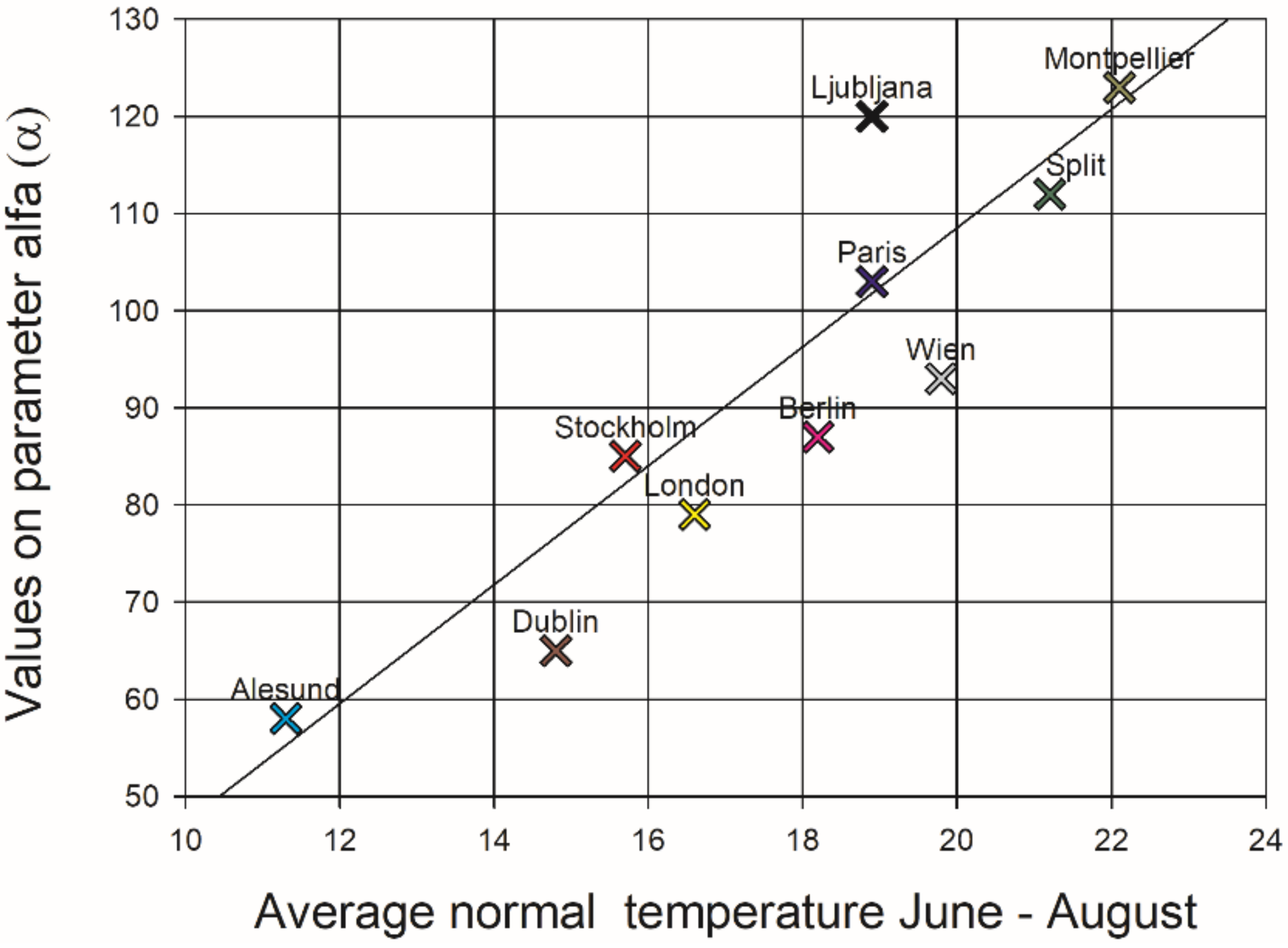
Equation (5) was then tested by investigation of the factor α with places with various temperatures with all other constants in the equation fixed. It turned out that the α-factor was highly temperature dependent, see Figure 3.
Figure 2 and Figure 3 indicate that the primitive Equation (5) returns IDF statistics of interest. The factor α generally increases as expected with a warmer climate. This factor is connected with the vertical magnitude of the clouds. With deeper clouds and warmer air, more latent heat can be released and larger amounts of precipitation can be produced. The simple factor for reduction of the buoyancy due to a combination of entrainment and the decrease of rain intensity with distance from the center of the rain shower seems to be at least plausible with this primitive model.
In summary, the above cloud and rainfall intensity study gives a strong impetus in the direction of the importance of coupling rain intensity to climatological factors.
2.2.2. Second Approach by Involvement of Climatological Parameters
Considerations. From the above cloud physical study it is evident that a potential exists for the use of climatological data for the estimation of intense rainfall. When describing the rain intensity climate in terms of frequency of intense rain events, it is important to have information on the degree of instability of the atmosphere. The precipitation depth gives relevant information on the stability conditions on a monthly and yearly basis. For European conditions, it is clear that, in general, the summer months with high temperatures will have the most favorable conditions for efficient convection and heavy rains. However, the temperature climate is not enough: it is well known that, in the Mediterranean region, the largest and most intense rainfall comes during wintertime with colder temperatures. Similarly, in some climatological regions, the oreigenic rainfall is dominating and can also occur at other months than during the summer.
The above considerations resulted in the following steps 1–3 for development of the primitive version of Equation (4) to an expression coupled to climatological data for a 30-year normal period in the point estimation of intense rainfall:
- The general efficiency of the formation of precipitation at a specific place is connected with the level of the annual rainfall amount. This parameter scales the climate from dry, desert-like conditions to abundant extreme tropical/monsoon precipitation. In the formula below, this parameter is denoted below as: RY (‘Rain amount for the Year’).
- The months with the highest rainfall amounts indicate when the largest instability of the atmosphere occurs. The two months with the most precipitation were selected and are denoted below as: R2, (‘Rain sum/2 months’).
- The air temperature is of importance for the water vapor-holding capacity of the atmosphere. The average temperature was selected from the two months with the largest rainfall sum and is denoted below as: T2, (Average Temperature/2 months).
Problems with the quality of rainfall intensity data are summarized in Section 2.1 with the items a–f. To handle these problems with systematic errors, a factor is introduced, where subscript ‘n’ indicates national influence regarding the data and their processing.
The second approach for the development of a formula, R, for intense rainfall is presented in Equations (6) and (7) below and can be regarded as a new approach largely independent of the previous Equation (4), presented in Section 2.2.1. The national factor An is introduced as well as the predictors 1–3 described above: RY, R2 and T2. The new expression contains two factors that also exist in Equation (4) developed by cloud physical considerations: (a) the formulation of the buoyancy force and (b) the expression for reduction of the buoyancy force (entrainment).
The coefficients were determined by use of a quasi-Newton [24] method for non-linear determination. The method starts with initial estimates of parameter values. These are then changed in small steps until the gap between the estimates and the input data is minimized. The initial values have to sometimes be changed to get convergence of the estimates. With this investigation, the start values were kept as few as possible at the beginning. The quasi-Newton method was then operated several times with an increased number of parameters to be determined. Comprehensive investigations ended with the best explained variance and with some adjustments of the maximum estimated values with the following formula R for the point rainfall amount. For the symbols used below see Table 1. The resulting estimates turned out to be underestimates and, consequently, an additional procedure was formulated to compensate for this problem, see ‘Correction of estimates’ below.
Correction of estimates:
Through the application of Equation (7), it turned out that the non-linear estimates resulted in underestimates as compared with the EVA data. A simple correction Δ of the estimates was introduced. mm, where D is the duration of the block rains. The Final Estimate = Estimate (by Equation (7)) + .
Table 3 gives basic information on the content of the datasets R1 and R2.
3. Results
3.1. The Developed Formula R in Comparison with the Outcome from Extreme Value Analysis
The basis for the present development of an IDF formula R consists of EVA data for geographic locations and of climatological norms for these places.
The present approach benefits from previous estimates made by the EVA type of statistics for locations in Europe, Southeast Asia and Australia.
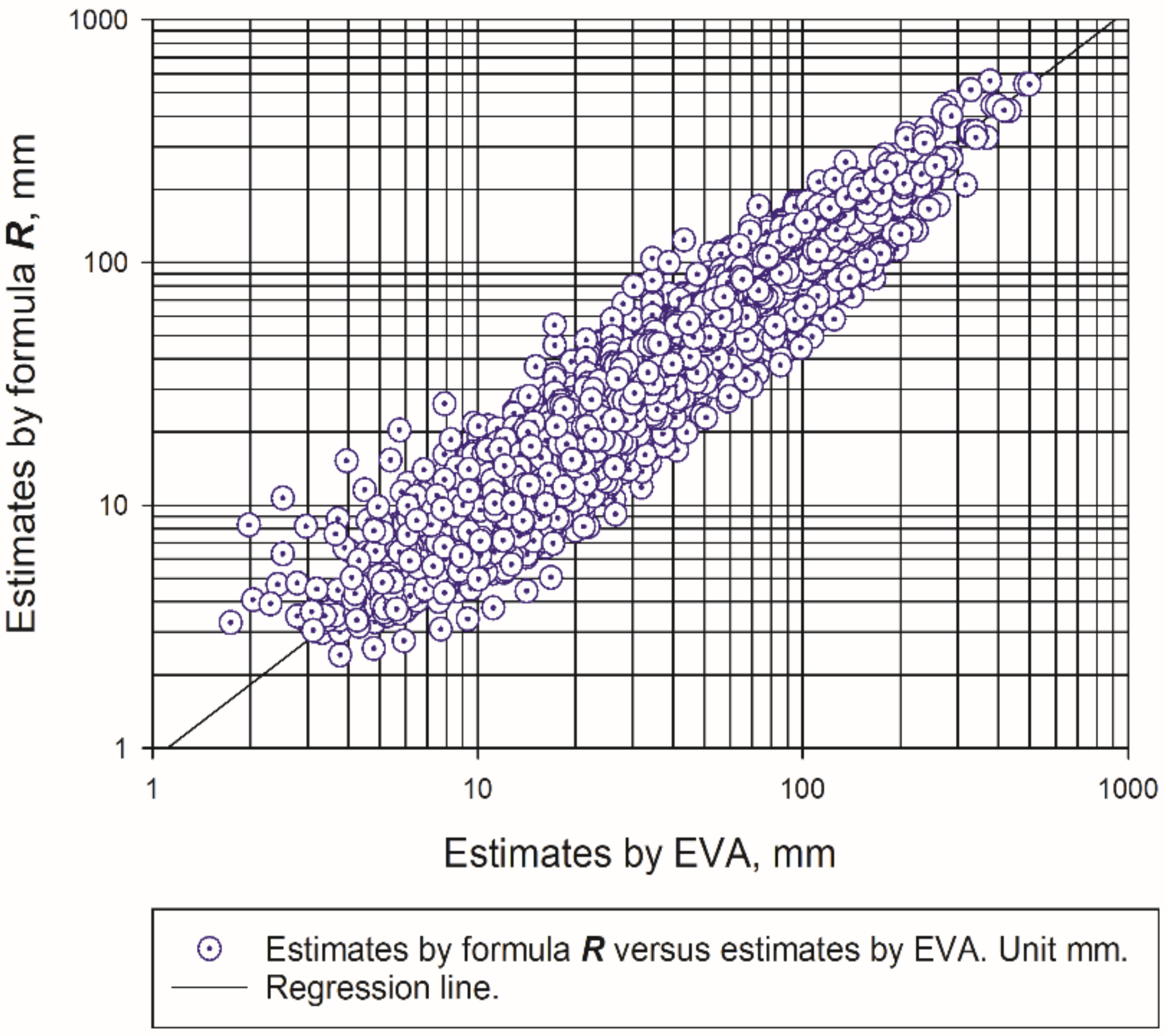
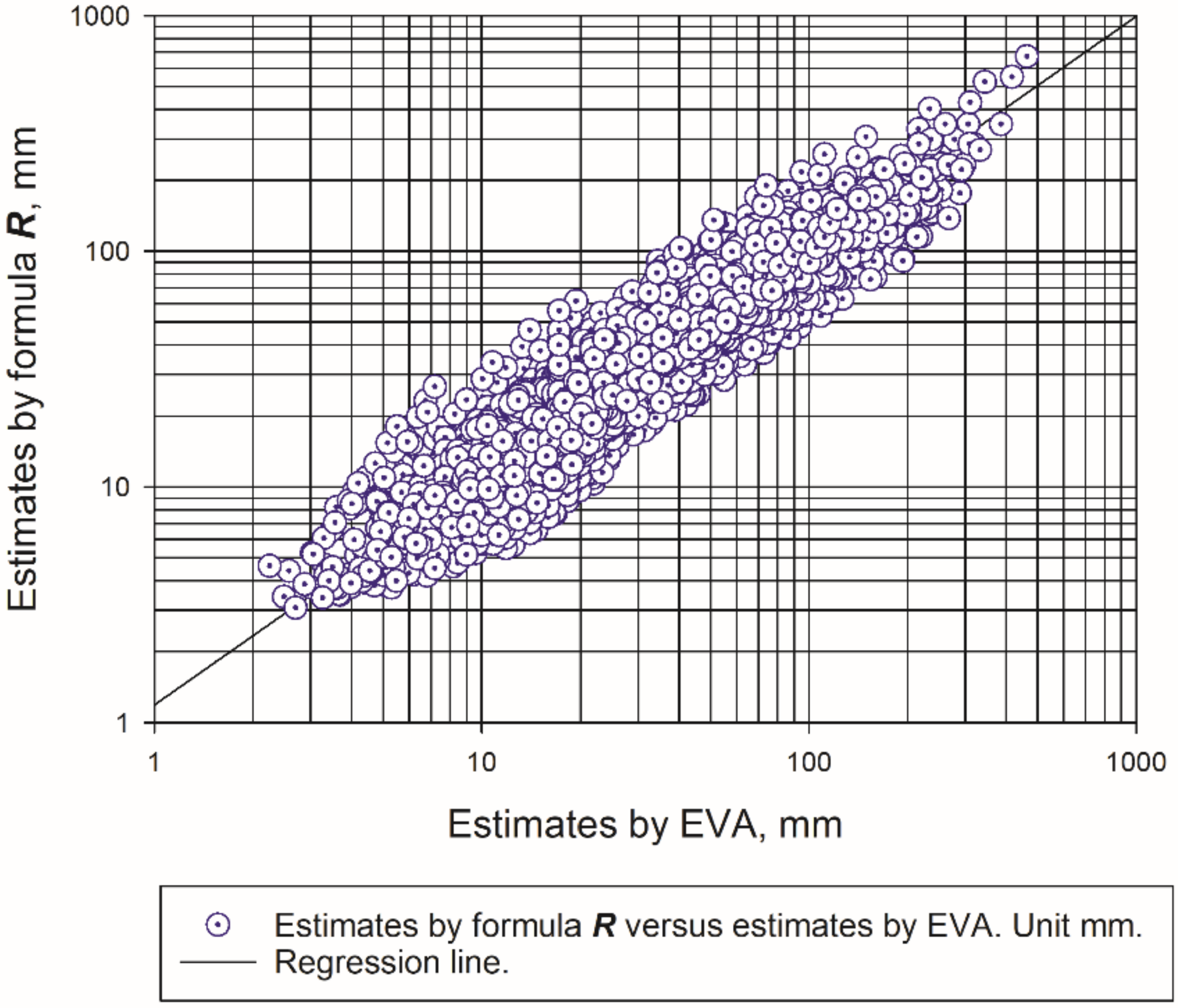
Figure 4 and Figure 5 illustrate the results of the main objective with the development of an IDF relationship based on climatological predictors.
The developed equation R is based on a non-linear estimation with data from 4132 rain intensity values, or “block rains”, in dataset R1. Dataset R2, for broader applications, covers locations with an average monthly normal temperature during the two wettest months extending from +9.7 °C to +29.0 °C. These data also cover a normal yearly precipitation sum extending from 302 mm to 2064 mm. The duration of the rainfall statistics (based on block rains) covers the time span of 5 min to 24 h. The variance of EVA data in the dataset R1 is explained by this relationship up to 90% (with the mean corrected explained variance at 79%) and in the independent dataset R2, it explains up to 90% (with the mean corrected explained variance at 80%).
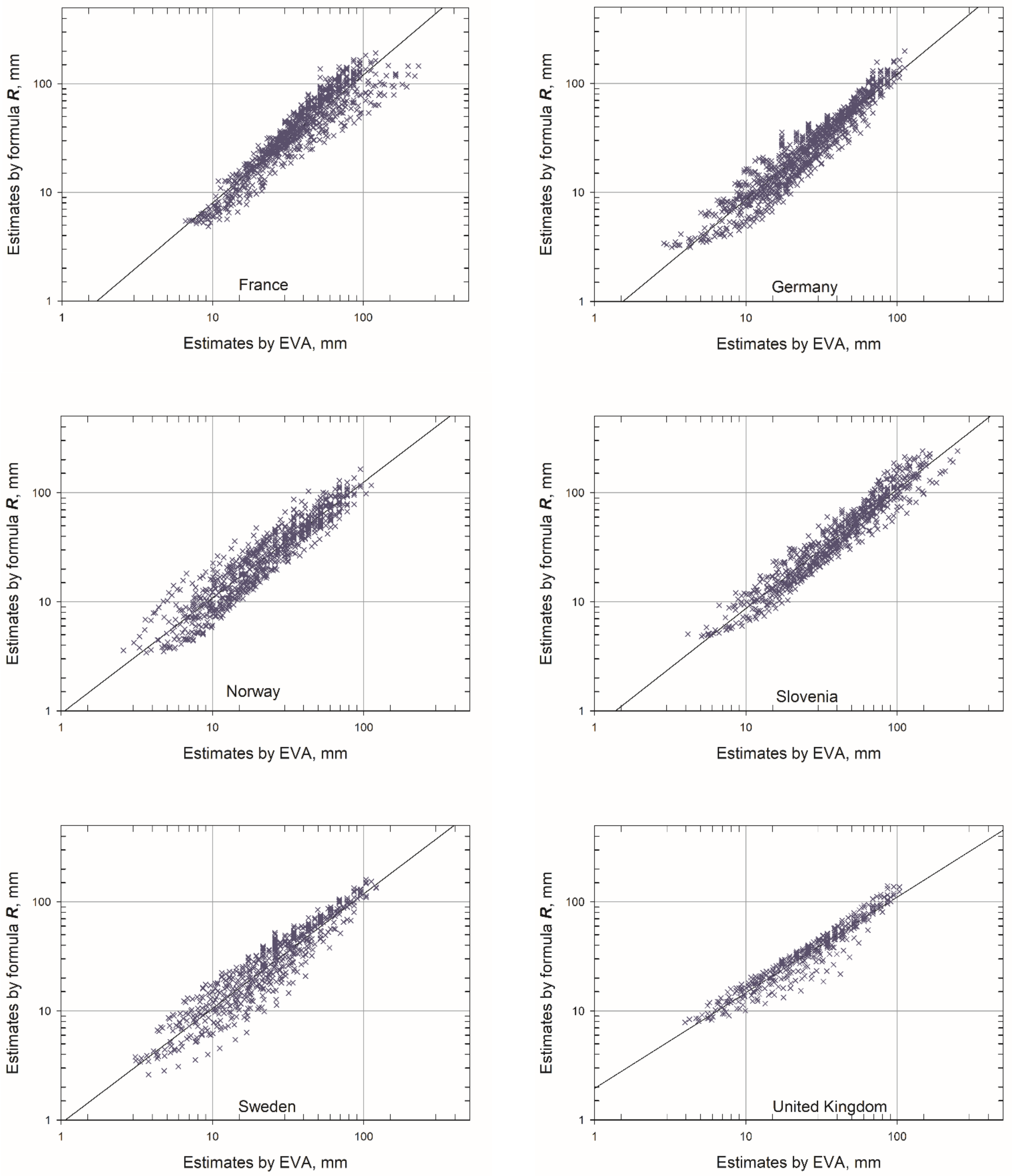
The developed formula R was applied on EVA data from some European countries. The results are presented in Table 4 and in Figure 6. The explained variance varies from 86% to 97%. The factor An shows a large variation from 0.80 (Norway) to 1.41 (Sweden). The reason for this large variation is not fully understood. Some of the national factors a-f in Section 2.1 give probable influences on the magnitude of An, but it can also be unknown deficiencies in the formula R that are the cause of the fluctuations of An.
Consequently, it is a recommended strategy to first determine the An coefficient by applying formula R with available EVA data and climate norms on the specific national data. All other coefficients are then kept unchanged at the estimation.
3.2. The Geographical Distribution of Rain Intensity by Use of Climatological Data as Predictors
With the equation for R, it is possible to use the climatological data to transfer this information to fields of rainfall intensity for various return periods and durations.
The steps are as follows:
- The factor An, regarding the national influence on the rain intensity estimates, has to be determined by matching the formula for R with the available EVA data from the studied country. A preliminary value of An can be set to 1.0.
- It is important to process the climatological data (temperature and precipitation) to climate normals, which generally is achieved on a routine basis in most countries.
- The predictors T2, R2 and RY (see steps 1–3 in Section 2.2.2) are evaluated for each climate station from the data on climate norms.
- With predetermined information on the duration and period of return (example: 5 min and 50 years), the formula R is processed by use of the values on the three predictors at each geographical point represented by the respective climate station.
- If more information is needed, then step 4 continues by selecting new predetermined values of the duration and period of return and processing the set of climate stations with formula R again.
Steps 1–5 above were applied with climatological data from Sweden (see Figure 7) and the use of the formula R. Figure 8a–d on the next pages illustrates the rain intensity and frequency maps for Sweden. The isoline patterns are produced by gridding the estimated rain intensity values of the climate stations by use of a Kriging technique and then proceeding with the creation of contour maps.
3.3. The Equation for R and Estimates of Probable Maximum Precipitation (PMP)
The probable maximum precipitation (PMP) is a theoretical concept that is widely used by hydrologists to estimate the probable maximum flood. The PMP finds use in planning, design and risk assessment of high-hazard hydrological structures such as flood control dams upstream of populated areas. The PMP represents the greatest depth of precipitation for a given duration that is meteorologically possible for a watershed or an area at a particular time of year. Various methods are in use for the estimation of the PMP over a target location [25].
The developed relationship R offers a point estimate of extreme rainfall quantities with adherent recurrence periods. Consideration of the traditional PMP methods and the areal distribution of a basin’s PMP involves the shape and orientation of its isohyetal pattern, and this may be based on observed storms. With the possibility to estimate years of recurrence, by use of climate norms, another perspective opens: with climate data, observed or interpolated over a basin, it is possible to transform this climatological field to a field containing isolines with years of recurrence.
The world records of intense rainfall [26] give a probable upper threshold of what levels of rainfall and PMP can be reached. Figure 9 illustrates the absolute world maximum rainfall of today together with one example of estimates that the formula R gives by regression of the parameter ‘return period’.
The property inherent with the formula R to determine the return period is believed to facilitate the decision-making process for investment projects, as the input data for operating the equation for R essentially comes from normal values of temperature and rainfall, which generally are available.
In Figure 10, the rain depths for recurrence of 1, 200 and 2000 years are illustrated for a selection of locations with the predictor T2 in the interval 15.0 to 15.9 °C. The recurrence is determined by use of equation R with the exponent 0.686, see the note in Table 2, Section 2.2.2. It is clear from this illustration that the level of world records (the top symbols and line) will hardly ever be reached at these locations. Depending on the wanted/expected life length of the actual investment type of object, it is possible to select the relevant curve for the determination of rainfall depths from Figure 10 or from other estimates generated by use of equation R.
As can be seen from Figure 10, it is unrealistic that rainfall at the selected locations will ever reach the level of global extreme cloudburst depths, represented by the top line The expected lifetime of the investment should be considered together with the information on the years of recurrence and the associated rain depth.
The use of PMP methods for the estimation of rain depths over a basin may result in high costs if the return period related to rain depth is not properly estimated. With the method presented here, estimates of the recurrence period of rainfall events are facilitated, and instead of applying estimates by PMP, an alternative is to pose the question of the expected, or required, lifetime of the investment. Example: a project may be designed to accommodate a rain depth with a return period of 100 years or 300 years, rather than to accommodate cloudburst depths based on the PMP that will physically never be reached and will likely incur substantially higher infrastructure costs.
Remark. Determination of estimates of the recurrence period and rain depth is inherent with the formula R, Equation (7). The method is proposed to be denoted like PMPny, where “ny” means the number of years of recurrence. PMP150 means the “PMP with recurrence 150 years”. Cost–benefit considerations with the PMP involved mean that, with PMPny, there is an improved potential for savings in energy and environmental costs with the improved possibility to identify the return period and the rainfall depth.
3.4. The Change of Rainfall Intensity Due to Climate Change
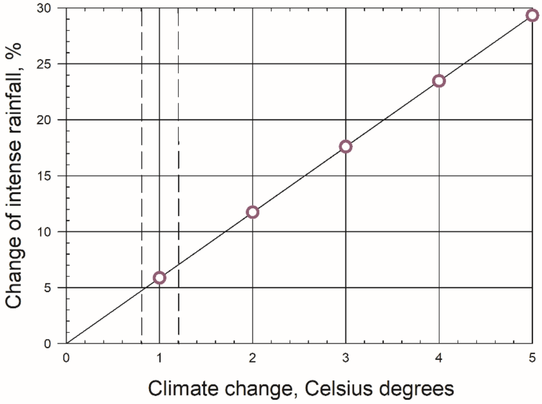
The relationship R, see Equation (7), contains three climate normal variables, temperature ”T2”, rainfall “R2” and yearly rainfall sum “RY”. Due to the ongoing of a global warming, it is of interest to examine how the rain amount is affected if the values of temperature or the rainfall in equation R are changed. In this investigation, the T2 values were increased stepwise by +1 degree up to +5 °C. Data from the combined dataset R1+R2 were used. The difference between the obtained rainfall depths caused by increased temperature and the values without temperature change were studied, see Figure 11 and Table 6.
It should be noted that this study concerns what happens with block rains (the intense part of a rainfall) if the temperature increases. The focus here is consequently not on general rainfall.
According to Clausius-Clapeyron’s (‘CC’) relation, the moisture holding capacity is about 7% per °C rise. Intensified rainfall at this level would be expected. The result shown in Figure 11 indicates an average increase of 5.87% per degree. The spread around this value is considerable, as seen in Table 6. The result supports the statement of the IPCC [28]: “Extreme precipitation events over most of the mid-latitude land masses and over wet tropical regions will very likely become more intense and more frequent”. More information on the result of the use of formula R and fictive temperature increases is contained in Table 6.
A dependency of hourly precipitation extremes on the daily mean 2 m temperature of about two times the CC relation has been reported [28]. From this paper, one conclusion is that this phenomenon is a result of changes in atmospheric stability, with higher temperatures leading to a larger instability. With more latent heat release, due to a higher water content, the formation of rain will be intensified.
To study this effect’s influence of higher temperatures on the efficiency of rain formation, the predictor T2 (temperature during the two wettest months) was increased by 1 °C in the datasets R1 and R2. No convincing results were obtained. Nevertheless, the interior dynamic and turbulent cloud processes, where channels of heavy rainfall interact, could tentatively be the cause of this phenomenon called super CC.
4. Conclusions
Risks of sewer overflow and flooding are increasing in a warmer world. The relationship, R, for the estimate of rain intensity and its time of recurrence is then a possible method to generate basic data for the design and planning activities in many regions.
- 1.
- The use of a mathematical expression R using climate norms as predictors for the estimation of extreme rainfall seems feasible: the variance in data from the extreme value analysis is explained by independent estimates up to about 90%.Numerical property. The coefficients in the formula are connected with climatological predictors: when the climate changes, the predictors (T2, R2, RY) will change, but the coefficients in formula R are expected to be relatively unchanged.Application domain. The application space of the formula, R, covers regions with a climatological normal temperature within at least +7 to +32 °C during the wettest two months, and within at least 300 mm to 2100 mm of the normal annual rainfall. The duration time of R covers 5 min to 24 h.
- 2.
- A key problem when processing rain intensity data is the fact that these data are influenced by a multitude of error sources, summarized in Section 2.1 of the present article. To reduce this problem, a screening technique by use of a national factor An, determined by regression, plays an important role in reducing and cleaning systematic errors.
- 3.
- Equation R increases the potential to estimate the appropriate return period and the connected rainfall depth for heavy and intense rainfall. Applications connected with the probable maximum precipitation then have an increased potential to be improved. The notation “PMPny“ is introduced just to accentuate the importance of the recurrence period for intense rainfall when planning investments in urban discharge systems or other infrastructure. This ability of the relationship R to estimate the return period of heavy rainfall results in an improved potential for savings in energy, investment and environmental costs of building infrastructure.
- 4.
- The effect of climate warming and changes of the rainfall amount is estimated by use of the equation R. It is concluded that an increase of 1 to 5 °C indicates on average an increase of 5.9% of the rainfall amount for each warming degree. This estimate concerns the most intense part of the rainfall (contained in the so-called ‘block rains’). It should be pointed out that the presented estimates are independent of the results obtained by dynamic models.
Supplementary Materials
The following are available online at https://www.mdpi.com/article/10.3390/w13162292/s1, File S1: Total Data.
Funding
The Swedish Water and Wastewater Association/Development contributed financial support with the Projects Nos: 29-103, 04-14 and 19-101. The European Weather Services kindly contributed rain intensity data to this project. We acknowledge the E-OBS dataset from the EU-FP6 project ENSEMBLES (http://ensembles-eu.metoffice.com, accessed on 2 July 2021) and the data providers in the ECA&D project (http://www.ecad.eu, accessed on 2 July 2021).
Institutional Review Board Statement
Not applicable.
Informed Consent Statement
Not applicable.
Data Availability Statement
All data needed to evaluate the conclusions in the paper are present.
Acknowledgments
I am grateful to Claes Hernebring, DHI, for his retrieval and handling of rain intensity data and data for selection of predictors and also for his knowledge and scrutiny of the paper together with Gilbert Svensson, “Vattenforum”, who also contributed to the focus on urban sector needs of rainfall information. Erik Kjellström, Rossby Centre, SMHI, went through the manuscript and brought forward a multitude of professional improvements. Gordon Anderson, MBA, IMD, Switzerland, provided language support.
Conflicts of Interest
The author declares that he has no competing interest.
References
- Willems, P.; Olsson, J.; Arnbjerg-Nielsen, K.; Beecham, S.; Pathirana, A.; Gregersen, I.B.; Madsen, H.; Nguyen, V. Impacts of Climate Change on Rainfall Extremes and Urban Drainage Systems; IWA Publishing: London, UK, 2012; Volume 11, ISBN 9781780401263. [Google Scholar] [CrossRef]
- Stocker, T.F.; Qin, D.; Plattner, G.-K.; Tignor, M.; Allen, S.K.; Boschung, J.; Nauels, A.; Xia, Y.; Bex, V.; Midgley, P.M. Climate Change 2013: The Physical Science Basis—Working Group I Contribution to the IPCC 5th Assessment Report; Cambridge University Press: Cambridge, UK, 2013. [Google Scholar]
- Hernebring, C.; Milotti, S.; Steen Kronborg, S.; Wolf, T.; Mårtensson, E. Skyfallet i sydvästra Skåne 2014-08-31 (The cloud-burst in southwestern Scania 2014-08-31). J. Water Manag. Res. 2014, 71, 85–99, (In Swedish with English Abstract). [Google Scholar]
- Fisher, R.A.; Tippett, L.H.C. Limiting forms of the frequency distribution of the largest or smallest member of a sample. Math. Proc. Camb. Philos. Soc. 1928, 24, 180–190. [Google Scholar] [CrossRef]
- Gnedenko, B. Sur la distribution limite du terme maximum d’uneserie aleatoire. Ann. Math. 1943, 44, 423–453. [Google Scholar] [CrossRef]
- Gumbel, E.J. Les valeurs extrêmes des distributions statistiques (PDF). Ann. De L’institut Henri Poincaré 1935, 5, 115–158. [Google Scholar]
- Fréchet, M. Sur la loi de probabilité de l’écart maximum. Ann. De La Société Pol. De Mathématique 1927, 6, 93–116. [Google Scholar]
- Weibull, W.; Rockey, K.C. Fatigue testing and analysis of results. J. Appl. Mech. 1962, 29, 607–608. [Google Scholar] [CrossRef]
- Dahlström, B. Regional Fördelning av Nederbördsintensitet—En Klimatologisk Analys (Regional Distribution of Precipitation Intensity—A Climatological Analysis); Report R18:1979; BRF: Stockholm, Sweden, 1979. [Google Scholar]
- Decker, F.W. Comments on the Adjectives “Oreigenic” and “Orograhic”. Mon. Weather. Rev. 1967, 95, 699. [Google Scholar] [CrossRef]
- Dahlström, B. Insight into the nature of precipitation—Some achievements by T. Bergeron in retrospect. In Weather and Weather Maps; Birkhäuser Verlag: Basel, Boston, 1981; pp. 548–557. [Google Scholar]
- Dahlström, B. Rain Intensity—A Cloud Physical Contemplation; Report 2010-05. The Swedish Water & Wastewater Association: Stockholm, Sweden, 2010. Available online: http://vav.griffel.net/filer/Rapport_2010-05.pdf (accessed on 19 August 2021). (In Swedish with English Abstract).
- Vatten, S. Svenskt Vatten Nederbördsdata vid Dimensionering och Analys av Avloppsvatten (Precipitation Data for Design and Analysis of Sewer Systems); Publication P104; Svenskt Vatten: Stockholm, Sweden, 2011. [Google Scholar]
- Hernebring, C.; Dahlström, B.; Kjellström, E. Regnintensitet I Europa med Fokus på Sverige—Ett Klimatförändringsperspektiv (Raifall Intensity in Europe with Focus on Sweden—A Climate Change Perspective); Report 2012-16; Svenskt Vatten Utveckling; Svenskt Vatten AB: Stockholm, Sweden, 2012. [Google Scholar]
- Olsson, J.; Södling, J.; Berg, P.; Wern, L.; Eronn, A. Short-duration rainfall extremes in Sweden: A regional analysis. Hydrol. Res. 2019, 50, 945–960. [Google Scholar] [CrossRef]
- Haylock, M.R.; Hofstra, N.; Klein, A.M.G.; Tank, E.J.; Klok, P.D.; Jones, M. A European daily high-resolution grid-ded dataset of surface temperature and precipitation for 1950–2006. J. Geophys. Res 2008, 113, D20119. [Google Scholar] [CrossRef] [Green Version]
- Asian Pacific FRIEND. Rainfall Intensity Duration Frequency (IDF) Analysis for the Asia Pacific Region; Trevor, M.D., Guillermo, Q.T., Eds.; IHP-VII; Technical Documents in Hydrology; Regional Steering Committee for Southeast Asia and the Pacific UNESCO Office: Jakarta, Indonesia, 2008. [Google Scholar]
- World Meteorological Organization; Allsopp, T.; Llansó, P. Guidelines on Climate Observation Networks and Systems; WMO/TD No. 1185; World Meteorological Organization (WMO): Geneva, Switzerland, 2003. [Google Scholar]
- Førland, E.J.; Allerup, P.; Dahlström, B.; Elomaa, E.; Jónsson, T.; Madsen, H.; Perälä, J.; Rissanen, P.; Vedin, H.; Vejen, F. Manual for Operational Correction of Nordic Precipitation Data; Nordic working group on precipitation; Report no. 24/96; Norwegian Meteorological Institute: Oslo, Norway, 1996. [Google Scholar]
- Taskinen, A.; Söderholm, K. Operational Correction of Daily Precipitation Measurements in Finland; Boreal Environment Research 21; Boreal Environment Research Publishing Board: Helsinki, Finland, 2016; pp. 1–24, ISSN 1797-2469. [Google Scholar]
- Dahlström, B. A General Classification of Error Sources in Rain Gauging and Some Applications; Nordisk Hydrologisk Konferens: Stockholm, Sweden; Nordisk Hydrologisk Förening: Lund, Sweden, 1970. [Google Scholar]
- Makkonen, L. Plotting positions in extreme value analysis. J. Appl. Meteorol. Climatol. 2006, 45, 334–340. [Google Scholar] [CrossRef]
- Ekroth, I.; Granryd, E. Tillämpad Termodynamik. Ph.D. Thesis, Linköping University, Linköping, Sweden, 2005; pp. 520–521. [Google Scholar]
- Fletcher, R. Fortran Subroutines for Minimization by Quasi-Newton Methods; AERE R. 7125; Atomic Energy Research Establishment: Harwell, UK, 1972. [Google Scholar]
- World Meteorological Organization (WMO). Manual for Estimation of Probable Maximum Precipitation; Publication No 1045; WMO: Geneva, Switzerland, 2009. [Google Scholar]
- World Meteorological Organization (WMO). Guide to Hydrological Practises, 5th ed.; WMO No. 168; WMO: Geneva, Switzerland, 1994; p. 403. [Google Scholar]
- IPCC. An IPCC Special Report on the Impacts of Global Warming of 1.5 °C above Preindustrial Levels and Related Global Greenhouse Gas Emission Pathways, in the Context of Strengthening the Global Response to the Threat of Climate Change, Sustainable Development, and Efforts to Eradicate Poverty. In 2018: Global Warming of 1.5 °C; Masson-Delmotte, V., Zhai, P., Pörtner, H.-O., Roberts, D., Skea, J., Shukla, P.R., Pirani, A., Moufouma-Okia, W., Péan, C., Pidcock, R., Eds.; Intergovernmental Panel on Climate Change: Geneva, Switzerland, 2019. [Google Scholar]
- Lenderink, G.; Van Meijgaard, E. Linking increases in hourly precipitation extremes to atmospheric temperature and moisture changes. Environ. Res. Lett. 2010, 5, 025208. [Google Scholar] [CrossRef]
Figure 1.
Example of identification of a block rain (in this case the maximum block rain) in a recorded rainfall event.
Figure 1.
Example of identification of a block rain (in this case the maximum block rain) in a recorded rainfall event.

Figure 2.
Illustration of the primitive relationship (5) with IDF data from London. The upper curves represent rainfall with a return period of 100 years and the lower curves represent 10 years of recurrence. Duration spans from 5 min to 24 h.
Figure 2.
Illustration of the primitive relationship (5) with IDF data from London. The upper curves represent rainfall with a return period of 100 years and the lower curves represent 10 years of recurrence. Duration spans from 5 min to 24 h.

Figure 3.
Examples of the variation of the factor alfa (α) in relationship (5). There is an indication of higher values of α with increasing average (June–August) normal (1961–90) temperatures.
Figure 3.
Examples of the variation of the factor alfa (α) in relationship (5). There is an indication of higher values of α with increasing average (June–August) normal (1961–90) temperatures.

Figure 4.
Dataset R1 for the development of the relationship R. This dataset consists of 70 locations and with 4132 pairs of estimated and corresponding EVA values.
Figure 4.
Dataset R1 for the development of the relationship R. This dataset consists of 70 locations and with 4132 pairs of estimated and corresponding EVA values.

Figure 5.
Dataset R2 for the application of the relationship R. This dataset consists of 78 locations with 4306 pairs of estimated and corresponding EVA intensity values.
Figure 5.
Dataset R2 for the application of the relationship R. This dataset consists of 78 locations with 4306 pairs of estimated and corresponding EVA intensity values.

Figure 6.
Examples of application of formula R on rain intensity information from some European countries.
Figure 6.
Examples of application of formula R on rain intensity information from some European countries.

Figure 7.
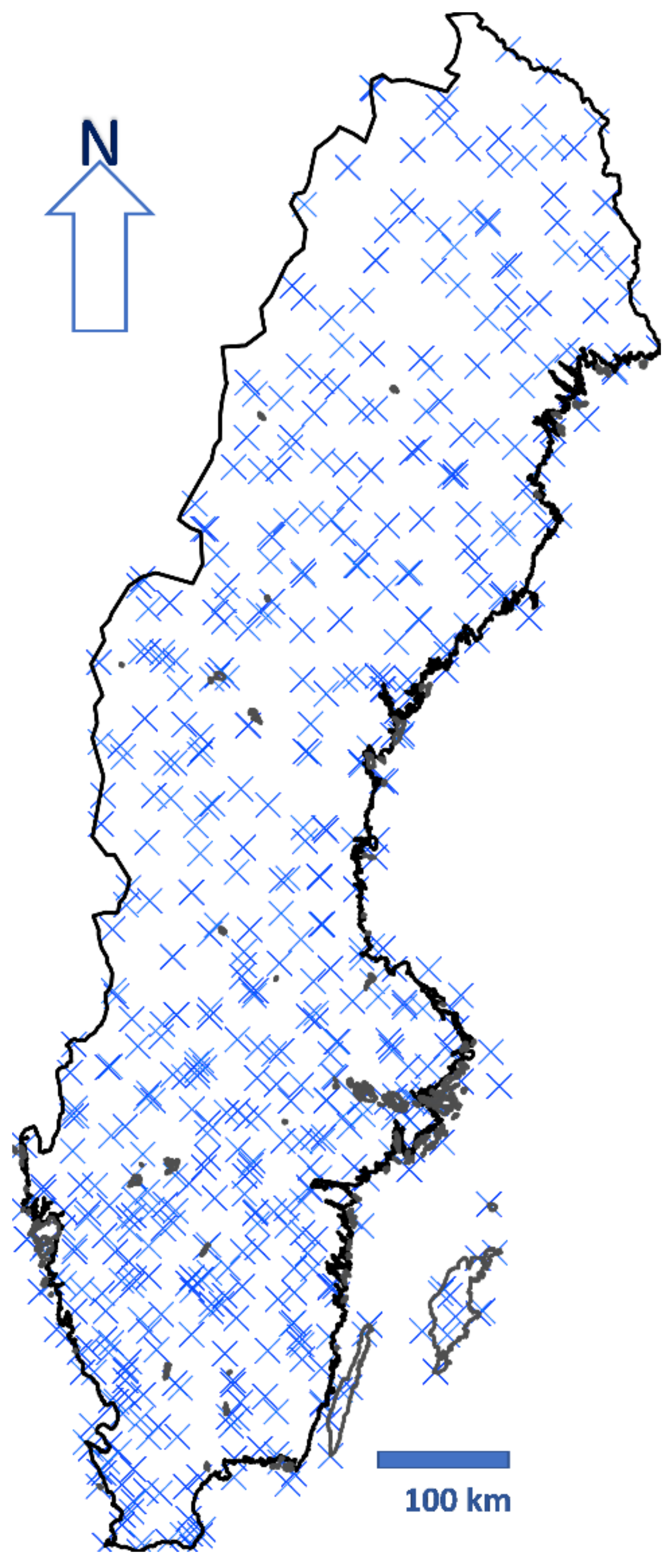
Part of the Swedish network of climate stations. These 588 stations were used for the development of the rainfall intensity maps 8a–d covering Sweden.
Figure 7.
Part of the Swedish network of climate stations. These 588 stations were used for the development of the rainfall intensity maps 8a–d covering Sweden.

Figure 8.
(a,b) IDF maps of Sweden based on the formula R. Map 8a illustrates the rainfall pattern with 10 min of duration and 10 years of recurrence. Map 8b illustrates 10 min of duration with 100 years of recurrence. Unit: mm. (c,d) IDF maps of Sweden based on the formula R. Map 8c illustrates the rainfall pattern with 60 min of duration and 10 years of recurrence. Map 8d illustrates 60 min of duration with 100 years of recurrence. Unit: mm.


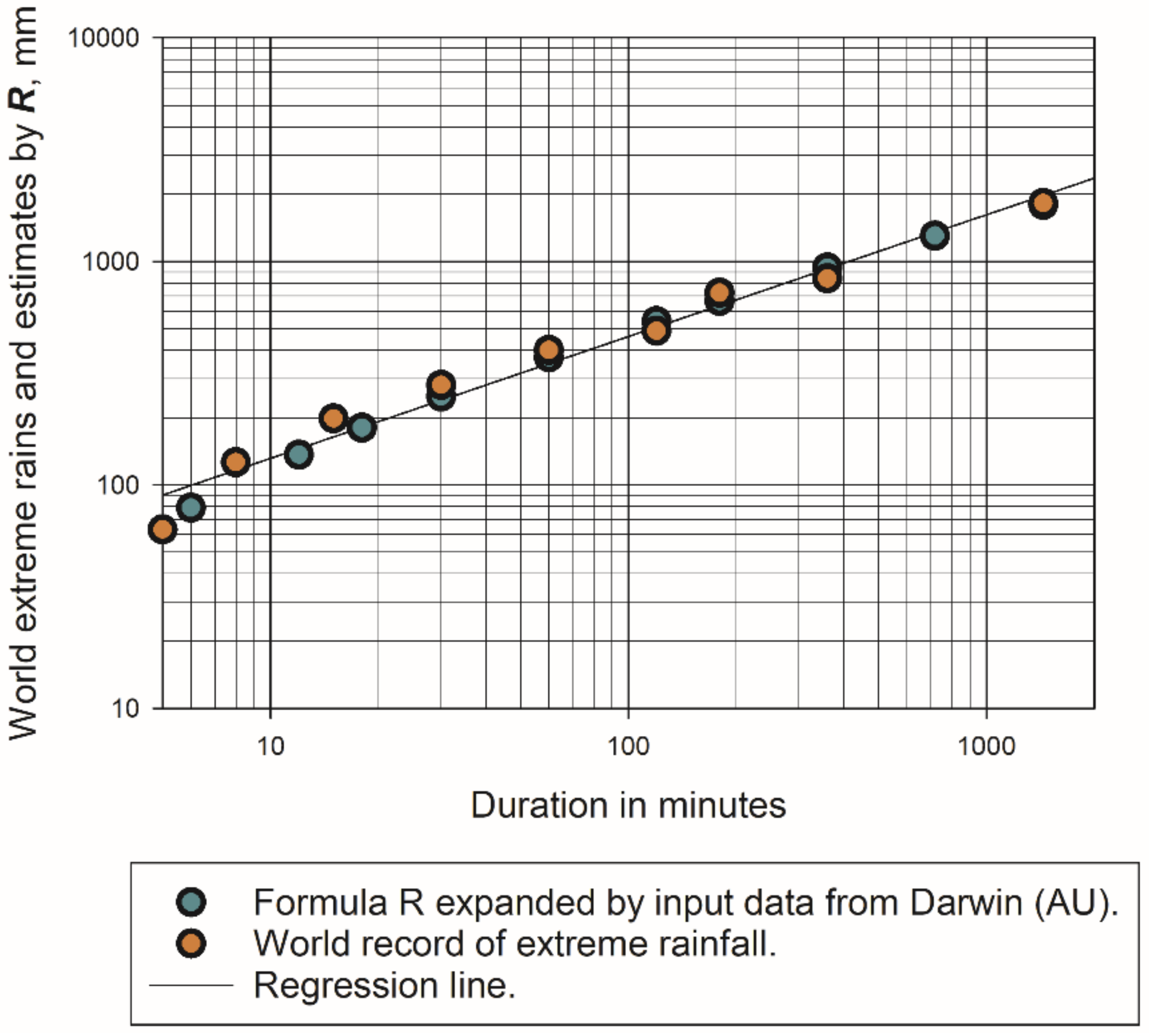
Figure 9.
World rainfall records vs. formula R applied on climatological data from Darwin, Australia: Data from Darwin was used with the relation R and with regression of the parameter ‘return period’. The return period obtained is 342 years (Wald confidence 95%, 321–363 years) with 99.6% explained variance.

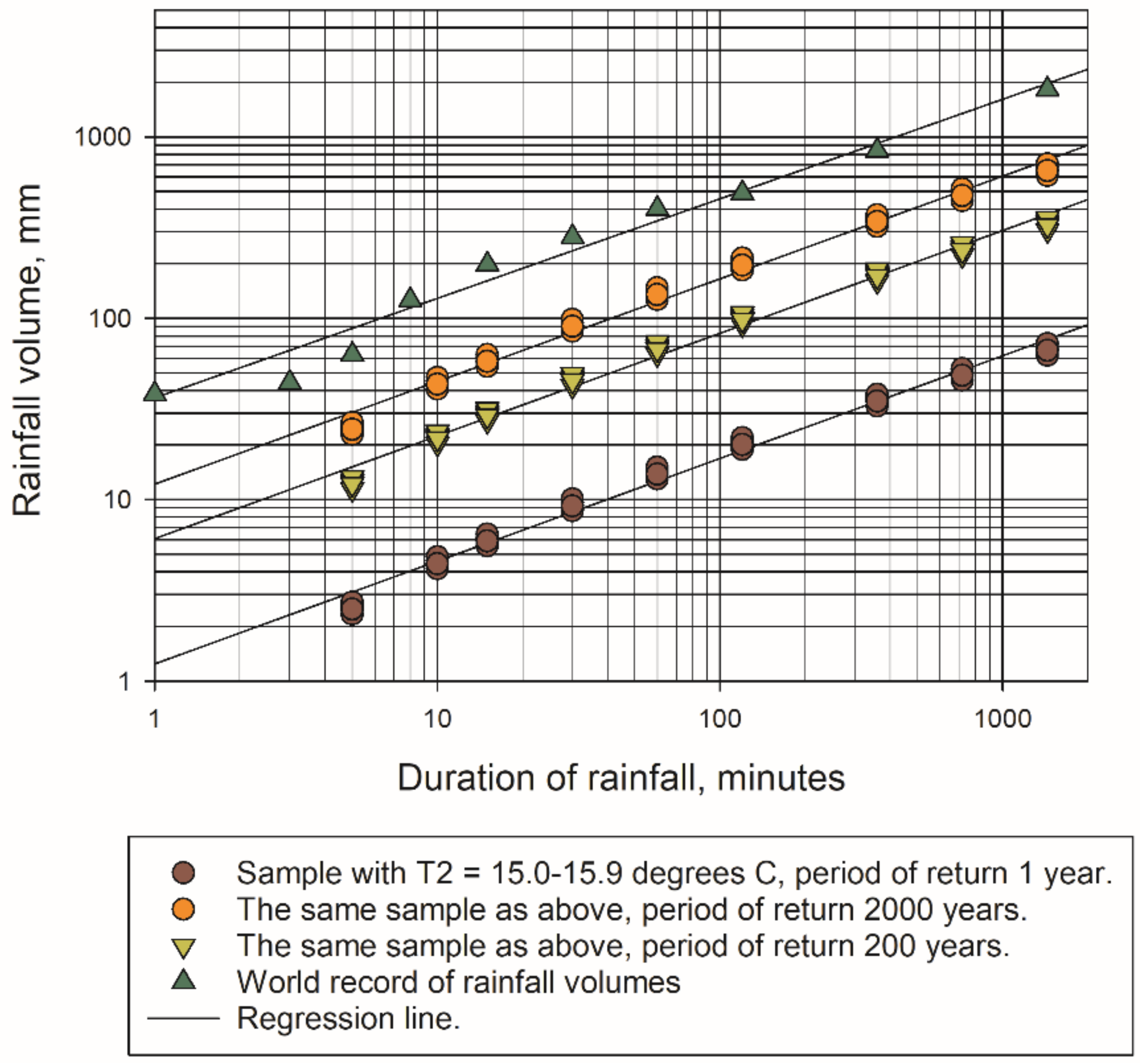
Figure 10.
Use of equation R for PMP purposes. Data from locations with temperature T2 in the interval 15.0 to 15.9 °C were extracted for this analysis. For the selected stations, see Table 5. The regression lines in the figure represent from the bottom up: 1 year, 200 years and 2000 years recurrence. The uppermost curve represents the world record of rainfall volumes.

Figure 11.
Change of intense rainfall depth in % due to change of the predictors of temperature in the equation for R: the predictor of temperature (T2) was increased by +1 to +5 °C and the change of the rainfall intensity was calculated using 8438 rain intensity values. Vertical lines: human activities are estimated to have caused approximately 1.0 °C of global warming above pre-industrial levels, with a likely range of 0.8 to 1.2 °C according to [27].


Table 1.
Explanation of symbols.
| Symbol | Explanation and Requirements—Temperature and Rainfall Values are 30-Year Climatological Norms |
|---|---|
| R | Rainfall amount in mm |
| Coefficients, see Table 2 below | |
| The temperature average (°C) of the two wettest months. A requirement is that T2 is above zero degrees. | |
| The sum of the two wettest rainfall months (mm). | |
| The yearly sum of precipitation (mm). | |
| Duration in minutes within interval: 5 to 1440 min (24 h). | |
| The recurrence period in months. |
Table 2.
Characteristics of the coefficients in the developed relationship
| An: For reduction of systematic er- rors. An is recommended to be cali- brated with national/regional data. | β and ε affect the general level of the esti- mates | γ influences the maximum estimated val- ues | δ δ also influ- ences the gen- eral level of estimates | ε a stable co- efficient in all tests | ζ Part of ex- ponent for D, dura- tion; see Equa- tion (7) | η Part of ex- ponent for D, duration; see Equa- tion (7) |
| Wald 95% confidence interval or ‘best estimate’ if the width of the interval coincides with zero. | 0.002 | 0.4 | 0.928–0.932 | 0.3 | 0.83 0.000026 For PMP 1 or for global rainfall estimates use exponent 0.686 instead of and no Δ-correc- tion | |
1 PMP, abbreviation for the probable maximum precipitation, cf. Section 3.3.
Table 3.
Information on the datasets R1 and R2.
| Dataset | Information on Predictors | Minimum | Maximum | Arithmetic Mean | Standard Deviation | Median |
|---|---|---|---|---|---|---|
| R1: | Normal temperature during wettest months (°C), “T2”. | 6.8 | 31.6 | 17.8 | 4.4 | 17 |
| Normal sum of rainfall during wettest months (mm), “R2”. | 53 | 853 | 258 | 164 | 207 | |
| Normal precipitation per year (mm), “RY”. 4132 values/70 locations | 404 | 2104 | 925 | 403 | 810 | |
| R2: | Normal temperature during wettest months (°C), “T2”. | 9.7 | 29. | 18.2 | 3.9 | 17 |
| Normal sum of rainfall during wettest months (mm), “R2”. | 53 | 871 | 233 | 123 | 208 | |
| Normal precipitation per year (mm), “RY”. 4306 values/78 locations | 302 | 2064 | 884 | 415 | 738 |
Table 4.
Examples of the application of formula for R in some European s countries. See also Figure 6.
Table 4.
Examples of the application of formula for R in some European s countries. See also Figure 6.
| Country | Explained Variance % | Factor An | Wald 95% Confidence Interval An | Number of Intensity Values |
|---|---|---|---|---|
| Sweden | 94 | 1.41 | 1.38–1.43 | 575 |
| UK | 97 | 1.06 | 1.04–1.08 | 391 |
| Norway | 92 | 0.80 | 0.78–0.81 | 809 |
| Slovenia | 92 | 1.10 | 1.07–1.12 | 692 |
| France | 86 | 1.12 | 1.09–1.15 | 879 |
| Germany | 92 | 0.91 | 0.89–0.92 | 1007 |
Table 5.
Locations of rainfall data for the PMP study illustrated in Figure 10.
Table 5.
Locations of rainfall data for the PMP study illustrated in Figure 10.
| Place | Country | Latitude | Longitude | T2 | R2 | RY |
|---|---|---|---|---|---|---|
| Stockholm | Sweden | 59.33 N | 18.06 E | 15.7 | 168 | 514 |
| Goteborg | Sweden | 57.71 N | 11.95 E | 15.7 | 207 | 782 |
| Växjö | Sweden | 56.88 N | 14.81 E | 15.9 | 189 | 638 |
| Cork | Ireland | 51.85 N | −8.49 W | 15.0 | 205 | 1027 |
| Askim | Norway | 59.59 N | 11.16 E | 15.2 | 245 | 829 |
| As | Norway | 59.67 N | 10.80 E | 15.5 | 235 | 810 |
| Gjettum | Norway | 59.91 N | 10.52 E | 15.2 | 247 | 832 |
| Herning | Denmark | 56.14 N | 08.97 E | 15.5 | 194 | 732 |
| Gdansk | Poland | 54.35 N | 18.65 E | 15.9 | 190 | 569 |
Table 6.
Increased rain amount in percent due to increased temperature. Results are based on 8438 rain intensity values.
Table 6.
Increased rain amount in percent due to increased temperature. Results are based on 8438 rain intensity values.
| Statistical Parameters | Temperature Change: Degrees CELSIUS: | ||||
|---|---|---|---|---|---|
| Unit: Percent (%) Relative to the Unchanged Climate. | +1 | +2 | +3 | +4 | +5 |
| Minimum | 3.17 | 6.32 | 9.49 | 12.66 | 15.82 |
| Maximum | 14.71 | 29.41 | 44.12 | 58.82 | 73.53 |
| Arithmetic mean | 5.87 | 11.73 | 17.00 | 23.46 | 29.33 |
Publisher’s Note: MDPI stays neutral with regard to jurisdictional claims in published maps and institutional affiliations. |
© 2021 by the author. Licensee MDPI, Basel, Switzerland. This article is an open access article distributed under the terms and conditions of the Creative Commons Attribution (CC BY) license (https://creativecommons.org/licenses/by/4.0/).
Share and Cite
MDPI and ACS Style
Dahlström, B. Cloud Physical and Climatological Factors for the Determination of Rain Intensity. Water 2021, 13, 2292. https://doi.org/10.3390/w13162292
AMA Style
Dahlström B. Cloud Physical and Climatological Factors for the Determination of Rain Intensity. Water. 2021; 13(16):2292. https://doi.org/10.3390/w13162292
Chicago/Turabian StyleDahlström, Bengt. 2021. "Cloud Physical and Climatological Factors for the Determination of Rain Intensity" Water 13, no. 16: 2292. https://doi.org/10.3390/w13162292
Note that from the first issue of 2016, this journal uses article numbers instead of page numbers. See further details here.