
Response of Zooplankton Size Structure to Multiple Stressors in Urban Lakes


1
School of Engineering, The University of Western Australia, 35 Stirling Highway, M051, Crawley, WA 6009, Australia
2
Research Centre for Limnology, Indonesian Institute of Sciences, Jl. Raya Bogor Km. 46, Cibinong 16911, Jawa Barat, Indonesia
*
Author to whom correspondence should be addressed.
Water 2021, 13(16), 2305; https://doi.org/10.3390/w13162305
Submission received: 2 July 2021
/
Revised: 12 August 2021
/
Accepted: 18 August 2021
/
Published: 22 August 2021
(This article belongs to the Section Urban Water Management)
Abstract
:Urban lakes are important environmental assets that contribute significant ecosystem services in urbanised areas around the world. Consequently, urban lakes are more exposed to anthropogenic pressures. Zooplankton communities play a central role in lake processes and, as such, are very sensitive to the impacts of human activities both through in-lake and catchment processes. Understanding their ecological function in urban lakes and how they respond to urbanisation is essential for environmental sustainability. In this study, we investigated the reliability of zooplankton size structure as indicators of anthropogenic stressors in urban lakes. We examined the relationship between environmental variables and zooplankton community size spectra derived as mean body size, density, and biomass. Our study showed that the overall mean body size was within the small size group ranged from 416 to 735 µm equivalent spherical diameter (ESD). Despite no significant difference in total zooplankton density between lakes, there was variability in the total density of the five different size classes. Total biomass was characterised by a significant proportion of size >750 µm. As the specific parameter of normalised biomass size spectra (NBSS), the slopes of the NBSS varied from moderate (−0.83 to −1.04) for a community with higher biomass of the larger size zooplankton to steeper slopes (from −1.15 to −1.49) for a community with higher biomass of smaller size. The environmental variables, represented by total phosphorus (TP) and chlorophyll a (chl-a), had a strong effect on zooplankton biomass and NBSS, where TP and chl-a were significantly correlated with the increase of total biomass and corresponded well with a less negative slope. Our results indicated that the community metric was sensitive to nutrient input and that size-based metrics have the potential to serve as key indicators for the management of urban lakes.
1. Introduction
Globally, freshwater ecosystems are increasingly under stress from urbanisation, and this is likely to increase as it is projected that more than 60% of the global population will live in cities by 2050 [1]. As urbanisation progresses, a key challenge for local city governments, communities, and scientists is to protect and maintain the ecological integrity of aquatic systems in the urbanscape [2,3]. The trends in urban densification due to population growth are projected to lead to a threefold increase in the urban land cover, leading to a disproportionately higher impact on environmental assets [2,4]. Effective conservation and management of urban ecosystems will increasingly rely on our ability to satisfy the demands of the growing population while maintaining the ecological integrity, thus maintaining the sustainable delivery of ecosystems services well beyond 2030. Furthermore, achieving the United Nations Sustainable Development Goals (SDGs) by 2030 will require a better understanding of the urban environment, which forms a critical pillar of sustainable cities and communities [5]. As stated by Seto, et al. [3], “cities can no longer be uncoupled from a full understanding of their ecological foundations”, of which aquatic systems are an integral part, in addition to other green infrastructure.
Aquatic systems in urbanised areas are arguably subject to more localised anthropogenic impacts due to land use changes and catchment characteristics, leading to hydrological regime fluctuations and increased transport pollutants [6,7]. They are also subject to broader impacts on regional and global scales, such as climate change [8,9]. Urbanisation has long been associated with a decline in water quality, leading to increased eutrophication and frequency of algal bloom events [10,11]. Additionally, there is evidence that eutrophication of freshwater systems is a leading cause of the changes in biodiversity [12,13]. Given these complex stressors, understanding community assembly and ecosystem functioning along environmental and urbanisation gradients remains a central topic in urban ecology, and there is room to study urban freshwater systems even further. While a growing body of research has addressed the significant impact of urbanisation on freshwater ecosystems, few of these studies have focused on urban and/or small lakes.
Urban lakes are defined as surface water bodies in an urban environment [14]. A recent definition of urbanisation has been expanded to include the increase in urban activities in more natural areas due to growing populations and economic development [15], meaning that the study of urban lakes may include lakes in more natural areas that are under increasing pressure from urbanisation. Urban lakes are usually small and shallow, and mostly man-made, but can range to highly modified natural systems, and provide a variety of benefits and services to both the community [16] and wildlife [17,18]. Urban lakes are important refuges for aquatic organisms [17,19] and frequently display high variability in community composition along spatial and temporal scales [20]. A large proportion of urban lakes (or ponds) are man-made and are highly regulated, which often lowers habitat quality because of the high influence of anthropogenic activities [21]. The combined impact of human activities, including high level nutrient and water pollution, habitat fragmentation, and biological invasion [22,23], has degraded many urban lakes to the extent that some are failing to provide sustainable delivery of resources and services [24].
Zooplankton, in particular, are a key element in aquatic ecosystems, including urban lakes, and have often been used in aquatic ecology research. Zooplankton act as intermediary species in food webs, facilitating energy transfer from the primary producers (phytoplankton) to a secondary consumer (predatory invertebrate and planktivorous fish), and are sensitive to environmental gradients and perturbation [25,26,27]. Given their essential role, changes in their community structure can lead to cascading impacts, which may affect both ecological organisation and ecosystem function [26]. Zooplankton can respond to bottom-up drivers, such as varying nutrient levels, and phytoplankton or cyanobacteria biomass [26,28], and top-down effects driven by planktivorous fish and macroinvertebrate predators, such as changes in species and community composition [29,30,31]. Moreover, many earlier studies have documented zooplankton community response to various environmental variables such as water chemistry, land use change [32], and urbanisation [33,34]. Given their essential role in aquatic systems and their rapid response to environmental changes, assessing the zooplankton community in urban lakes may reflect the impact of urbanisation on a system.
Assessing zooplankton community structure has recently shifted from solely focusing on species diversity (e.g., species composition and species richness) towards additionally including functional traits such as morphology, physiology, and body size spectra [29,35,36,37]; this increases our ability to investigate more integrative ecosystem processes. Body size index can be a critical indicator as many functional traits such as those that are ecophysiological and evolutionary are body size-dependent [38,39,40]. Size-based responses have been applied in many ecological studies linking the community size spectra, such as mean body size, size diversity, and biomass size spectra, with various environmental factors in different types of ecosystems, including marine and lake ecosystems [31,41,42]. Zooplankton community size structure has been linked to eutrophication processes [28,43,44,45], prey–predator relationships [31,46], the impact of invasive species [47], or a combined effect of both predation and cyanobacteria [48]. The growing amount of research on zooplankton community size structure clearly indicates that the size spectra of aquatic organisms, such as zooplankton, has potential as a robust indicator for community structure changes as a response to environmental stressors in urban lakes.
The overarching objective of this study is to examine zooplankton community structure, derived from high-resolution laser optical plankton counter (LOPC) measurements, and its relationship with environmental stressors in urban lakes. More specifically, the aims of this study are as follows: (1) to estimate the size and biomass of zooplankton communities using the LOPC equipped with lab circulator, (2) to assess the role of a selection of environmental factors and stressors on zooplankton community size structure in seven urban lakes, and (3) to assess the sensitivity of normalised biomass size spectra (NBSS) slopes to changes in the lake trophic level, as indicated by nutrients. The approach of combining LOPC data, advanced post-processing analyses, and NBSS is highly innovative and will lead to a better assessment of environmental change in urban lakes, which are highly valued ecosystem service providers.
2. Materials and Methods
2.1. Study Areas
The wetlands of the Swan Coastal Plain (SCP) in Western Australia support a diverse range of terrestrial and aquatic biota. However, increasing urban, agricultural, and industrial development over the past century has significantly reduced the number of wetlands that once existed on the SCP. The wetlands are subject to nutrient enrichment and pollutant contamination, and the wetlands have also undergone significant changes in hydrological regimes, owing to the combined effects of land use changes, drainage and damming of the rivers, and reduced rainfall in the last 40 years [49,50]. Additionally, clearing of native vegetation in the catchment, together with the decrease in river discharge, has led to a decrease in water level. Agricultural activities in the catchment also contribute to increasing nutrient loading of the wetlands, which is further exacerbated by urban nutrient loading from the Perth metropolitan area. The remaining SCP wetlands are mostly small and fragmented, as the landscape is dominated by partially cleared grazing land, agricultural areas, vegetated areas, industrial estates, and urban dwellings [19], and thus characterised by a high nutrient concentration [49].
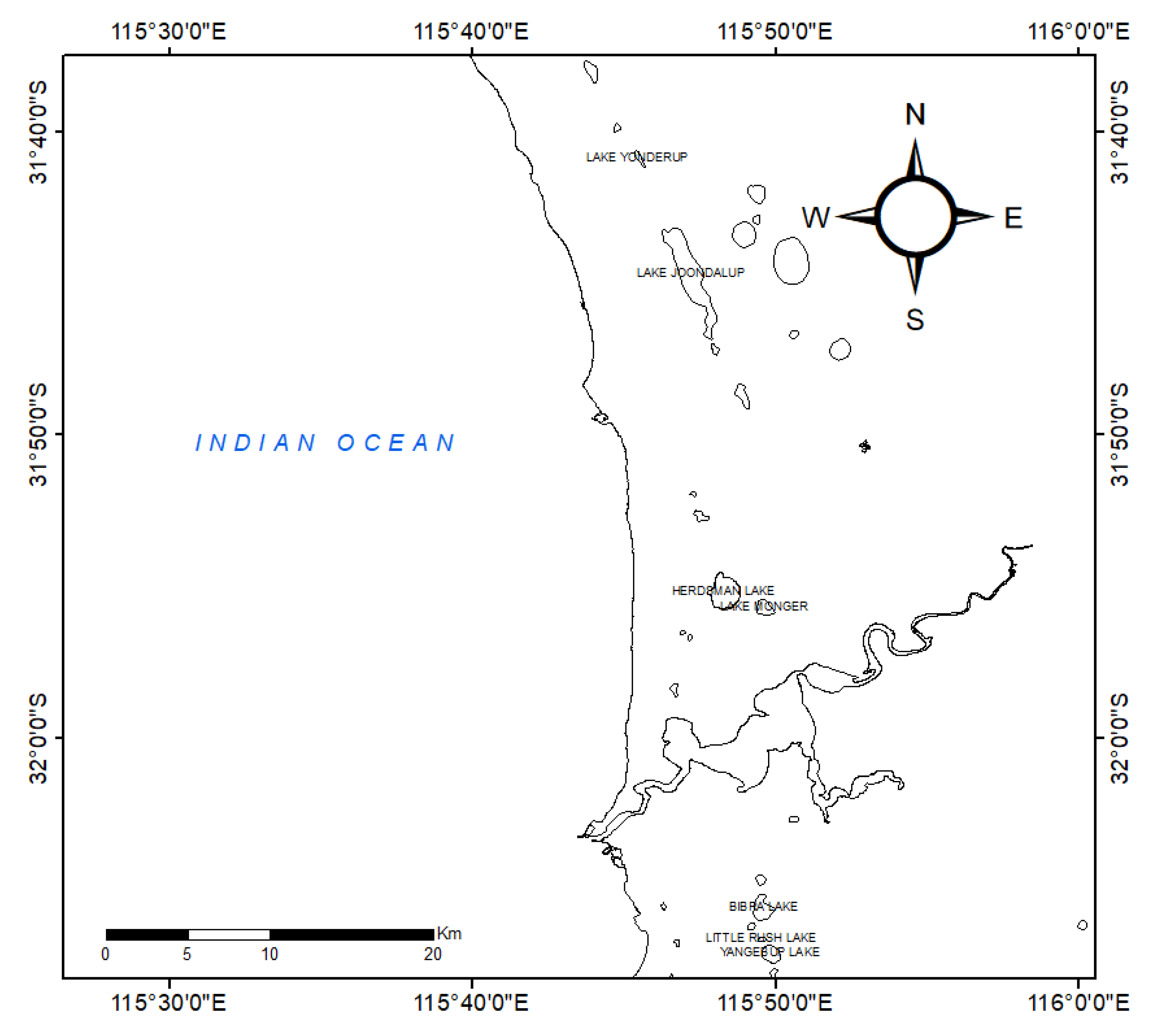
Seven urban lakes in Perth urban and peri-urban areas along the SCP (Figure 1) were selected for this study: Yangebup Lake, Little Rush Lake, Bibra Lake, Herdsman Lake, Lake Monger, Lake Joondalup, and Lake Yonderup (Table 1). The region is associated with a Mediterranean climate with hot, dry summers (December–February) and mild, wet winters (June–August). The hydrology of the study lakes is mainly influenced by the rainfall regimes and seasonal hydrological cycles. In most of the lakes, the maximum water levels usually occur in September to October, while minimum water levels occur at the end of the summer months in February [50]. Bibra Lake, Little Rush Lake, and Lake Joondalup temporarily dry up during summer, while the water level in Lake Monger is artificially regulated during summer months. Throughout the sampling period (2015 to 2016), the mean maximum annual temperature in the region was reported as 24.7 °C, with the monthly maximum temperatures being 30.1, 25.3, 19.5, and 25.4 °C for summer, autumn, winter, and spring, respectively [51]. Thermal stratification was not observed in any of the studied lakes, mainly because of continuous and intermittent wind mixing, creating homogenous physicochemical conditions throughout the water column.
2.2. Sampling and Analysis
All seven lakes were sampled during spring (September to early November) in 2015. Physicochemical variables such as temperature (°C), dissolved oxygen (DO, mg L−1), conductivity (µS cm−1), and pH were measured in situ using a WP-81 portable multi-probe water quality checker (TPS Pty Ltd., Brendale, Australia). Water transparency was estimated as Secchi depth. Three to four sampling points in each lake were randomly selected depending on the size of the water bodies with two replicates for each sampling point. Maximum air temperature on each sampling location recorded by the closest Bureau of Meteorology weather stations was used as a substitute for water temperature, as it was found that the onsite water temperature measurement varied depending on the time of sampling. Water samples were analysed for nutrient variables: total nitrogen (TN) concentrations were analysed with persulfate digestion method according to Hach Test ’N Tube (TNT) method 10071 for low range TN, while total phosphorus (TP) concentrations were analysed with the acid persulfate digestion method according to TNT method 8190 for low range TP. Both methods were previously validated against the standard methods according to the American Public Health Association [52]. Total concentrations of chlorophyll-a (chl-a) were measured a FluoroProbe (BBE Moldaenke, Schwentinental, Germany) configured for benchtop use. The FluoroProbe measures the chl-a fluorescence emission spectrum of four different groups of phytoplankton (chlorophytes, cryptophytes, diatoms, and cyanobacteria). The accuracy of the FluoroProbe for chl-a quantification was validated against values obtained from acetone extracted samples according to standard methods [52].
Zooplankton samples were collected at each lake by horizontal tow using a 56 µm mesh net and mouth diameter of 25 cm for a distance of 3 m at a constant speed of approximately 0.5 ms−1. Two horizontal tows from different directions were collected and pooled for each sampling point. Where water depth was low (below 0.5 m), a 50 L water sample was collected using a 5 L bucket and filtered using a 56 µm plankton net. All samples were further filtered onsite using a 250 µm mesh net to remove small particles (debris), concentrated to 150 mL and fixed with 4% sugar buffered formalin solution for further analysis.
2.3. LOPC Calibration
Prior to using the LOPC equipped with a sample circulator (Rolls-Royce Naval Marine Canada, Peterborough, Canada), to estimate zooplankton density and biomass, laboratory calibration was performed to validate that the LOPC could accurately estimate the size of various zooplankton groups against the manually measured zooplankton size under microscope.
Manual measurement and identification under a microscope were done prior to calibration of the LOPC. A fraction of zooplankton samples were manually sorted and classified into two taxonomic groups, cladocerans and copepods, and three size classes, consisting of large and small size cladocerans and copepods. The size (body length and width) of at least 30, and up to 100, organisms of each group was measured. Cladoceran body length was measured from top of the head to the spine tail excluding the spine, while the width was measured at the widest point perpendicular to the length. Copepod body length was measured for the total length of each individual excluding caudal setae, while the width was measured at the widest point of abdominal section perpendicular to the length. The measurements were conducted using a light dissecting microscope using a calibrated ocular micrometer against an objective micrometer. The mean equivalent spherical diameter (ESD) of zooplankton in each size group was calculated based on the following regression equation, as used in Zhou, et al. [53]:
where GM is the geometric mean of each zooplankton individual based on length and width measurements; GM is expressed as (length × width)0.5 [54].
Thirty to 100 individuals of the three zooplankton size classes (large-sized daphnia, small cladocerans, and copepods) were introduced through a sample chamber and passed through the LOPC to obtain data of counts and biomass of each size group. Data of zooplankton abundance (particle counts) and size (ESD, µm) of groups collected from the LOPC and microscopic examination were compared and then plotted and fitted to a linear regression model to assess the fitness between the two estimates.
2.4. Zooplankton Density and Biomass
Zooplankton mean size, density, and biomass were estimated using an LOPC equipped with a lab circulator. The collected density and biomass data were based upon particle density and biomass of 15 µm bin size, which were further binned into every 105 µm ESD intervals for the size range between 300 and 2500 µm ESD for further analysis. Although the LOPC measures particles from 100 to 3500 µm ESD size, we only analysed density and biomass for the zooplankton size range between 300 and 2500 µm ESD, as we found that air bubbles in the sample circulator prevented accurate counts for particle size <300 µm and extremely low density of zooplankton larger than 2500 µm ESD. Zooplankton density, mean body size, and biomass were determined per volume of water sampled. Density is the total abundance of all zooplankton detected per unit volume of water sampled, while mean body size is the average size of all measured ESD values. Biomass values were calculated using a method developed by Yamaguchi, et al. [42], in which the biomass present in each 15 µm size bin was calculated using the following equation:
The biovolume of each size bin was converted to wet biomass, assuming the specific gravity of zooplankton to be equal to that of water. Wet mass was then converted to dry biomass using a multiplier of 0.1, with the assumption that the water content of zooplankton is 90%. All size bin biomasses were summed to obtain the total biomass.
Zooplankton community size structure was initially examined as density and biomass distribution in 105 µm bin size intervals for size fractions between 300 and 2500 µm to examine the variation of community size structure in all studied lakes. This step also allowed us to determine mean body size for the entire lake based upon the density (ind L−1) data. For further analysis, the density and biomass estimates were then summed and classified into five ESD size groups (300–500, 501–750, 751–1000, 1001–1500, and 1501–2500 µm) to allow for a more functional classification. For each size group, density, and biomass value, the proportion of each size class to total biomass was determined for each studied lake.
2.5. Normalised Biomass Size Spectra
The biomass size spectrum was determined by binning the size biomass data for particle sizes between 300 and 2000 µm ESD into a series of logarithmically equal size intervals, which resulted in 26 bins. These biomass size spectra were then normalised by dividing the biomass in each bin by the width of the bin. The normalised biomass size spectra (NBSS) slope was derived by a least-square linear regression. The regression coefficient (R) of the linear fit of the NBSS slope was used to define the linearity of the NBSS slope, while the NBSS intercept is the y-intercept of the NBSS slope.
2.6. Statistical Analysis
Spatial variations in environmental variables and zooplankton size spectra (mean body size, total density, and total biomass) were determined using a non-parametric one-way ANOVA with Fisher’s least significant difference post hoc test. A multivariate ordination technique was performed to identify and visualise environmental variation and zooplankton size distribution in all seven lakes based on zooplankton numerical density (ind L−1) data in each 105 µm bin. Multiple linear regressions with backward selection were used to identify environmental variables that could best explain the variations in zooplankton size spectra. Zooplankton mean size, total density and biomass, and the density and biomass of five different size fractions were used as response variables, while chl-a, TN, TP, temperature, and Secchi depth were used as explanatory variables. All non-parametric, descriptive, and regression analysis were performed with SigmaPlot (version 14.0, Systat Software, Inc, Chicago, USA). Prior to statistical analysis, all continuous environmental variables were log10 transformed, while zooplankton density and biomass data were log10(1+x) transformed in order to meet the assumption of normality. The threshold of significance was set at 0.05 and a practical actual p-value was included. All multivariate analysis were performed using the Multi-Variate Statistical Package (MVSP; version 3.2, Kovach Computing Services, Pentraeth, UK) or R, and all variables were centered and standardised prior to principal component analysis (PCA) ordination.
3. Results
3.1. General Environmental Characteristics
A summary of the statistics of the 11 environmental variables measured in seven lakes is presented in Table 2. Lake open water area ranged from 0.0057 km2 to 4.55 km2, covering small to large lakes situated in mostly urbanised areas. Secchi depth and average water depth differed among lakes. Field sampling was conducted during spring (September to November 2016) when maximum air temperature ranged from 20.3 to 24.2 °C, and significant differences between lakes were observed. Mean conductivity differed significantly among lakes ranging between 0.71 and 2.17 mS cm−1. Mean salinity in all lakes also varied significantly with higher salinity observed in Lake Yangebup and Joondalup, mean salinity being 1229 ppm and 1012.62 ppm, respectively. All lakes were considered eutrophic based on the concentration of total phosphorus (TP) >30 µg L−1 [55]. Eutrophication indicators showed large gradients in the data sets, including TP ranging from 0.21 to 0.81 mg L−1 and TN from 0.10 to 2.75 mg L−1, water transparency (measured as Secchi depth) ranging from 0.5 to 0.9 m, and chl-a concentration varying from 1.92 to 24.95 µg L−1. One-way analysis of variance (ANOVA) showed a significant difference in TN, TP, and chl-a between lakes (all p < 0.05). A PCA ordination using all environmental variables (Figure 2) revealed that ~30% of the variability in environmental characteristics was explained by eutrophication indicators including chl-a, TP, pH, and Secchi depth, while ~26% was explained by other variables including suspended solids, temperature, DO, mean depth, salinity, and conductivity.
3.2. LOPC Validation
Linear regression analysis indicated no significant differences (p > 0.05) between the LOPC counts and ESD estimates, and direct zooplankton counts and ESD calculations, based upon zooplankton body width and length measurements (Table 3). There was a strong positive correlation between the LOPC-estimated ESD and directly calculated ESD, based upon body length and width measurement for all three zooplankton size classes, when assessed as both individual groups and as one single group in one analysis (Figure 3). The difference in zooplankton counts (abundance) by LOPC for both copepods and daphnia groups was relatively small, and is most likely due to sample losses or the sample being recounted during sample processing. This calibration procedure clearly indicates that the LOPC can be used with high confidence to collect and obtain high resolution data of zooplankton density and biomass.
3.3. Community Structure
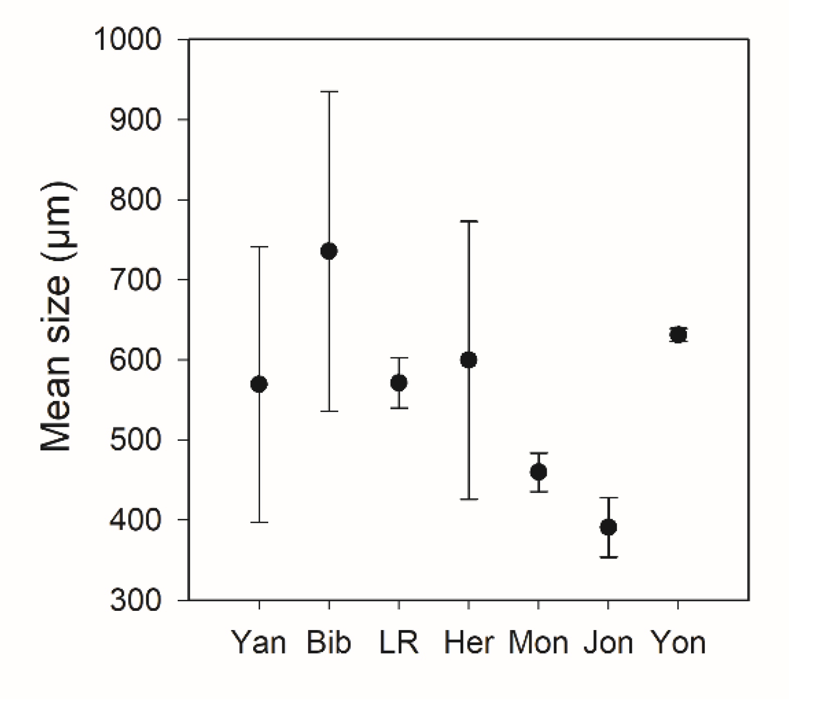
The summary of zooplankton community size spectra is presented in Table 4. Overall, the zooplankton communities in the seven urban lakes were characterised by a high density of small zooplankton fractions (from 300 to 750 µm), as shown by the PCA ordination based on zooplankton density in 105 µm bins, in which most lakes were oriented toward the 300–1000 µm size group (Figure 4a,b: 55–57% variation explained). Zooplankton mean body size was highest in Bibra Lake (735 µm ESD) (Figure 5) and there was significant difference in mean body size between lakes (ANOVA, p = 0.023). There was no significant difference in total zooplankton density (ind L−1) between lakes (p = 0.51); however, the variability in total biomass shows a significant difference between lakes (ANOVA, p < 0.001), with the highest biomass observed in Herdsman Lake (Table 4).
The zooplankton communities were also examined in further detail, in which the abundance and biomass of five size groups were considered, and differences in size distribution were evident. Small-sized zooplankton (from 300 to 750 µm ESD) were most abundant in all study lakes, except Lake Yonderup, where those of sizes between 500 and 1000 µm were significantly higher. The density of larger size fractions (>1000 µm ESD) was relatively low in all lakes, and in particular was the lowest in Lakes Monger and Joondalup, where the >1000 µm ESD fraction was less than 10% of the total density (Figure 6a,b). In contrast, the density of the size larger than 1000 µm ESD fraction was somewhat higher in Lake Yangebup, Bibra, and Herdsman than in other lakes. As confirmed by the size-based ANOVA analysis, a significant difference in the density of larger size group between lakes was observed (p < 0.001). Total biomass was primarily aggregated in the >1000 µm ESD size fraction. More than 50% of the total biomass over all seven lakes was aggregated in the 750–2500 µm ESD fractions. Biomass in Yangebup, Bibra, and Herdsman was significantly higher than total biomass in Little Rush, Monger, Joondalup, and Yonderup (Figure 6c,d).
3.4. Normalised Biomass Size Spectra (NBSS)
The results of the NBSS for each lake are shown in Figure 7. The slope of the NBSS ranged from −0.83 up to −1.49; significant inter-lake differences were observed for the slope (Table 4). Lakes with a moderate slope (−0.83 to −1.04) were significantly different from those with a steeper slope (−1.15 to −1.49). Lake Yangebup, Bibra Lake, Little Rush Lake, and Herdsman Lake had moderate slopes at −0.83, −1.04, −0.95, and −0.99, respectively, and this coincided with higher biomass of the size >1000 µm in these lakes. Lakes Monger and Joondalup, on the other hand, had steeper slopes at −1.49 and −1.41, respectively, and this correlated with the higher biomass of the smaller size zooplankton (300–500 µm). Lake Yonderup had a slightly moderate slope at −1.15 and was significantly different from the other lakes, in which the biomass of the intermediate size (500–1000 µm) had the highest contribution. When the NBSS was constructed for all lakes combined in one analysis, the average slope was somewhat steeper at −1.16, which indicates that the overall biomass in these lakes is characterised by small-sized zooplankton.
3.5. Environmental Variables Affecting Zooplankton Community Structure
The multilinear regression model explained 58% of the variance in mean body size (R2adj = 0.69, p < 0.001), with chl-a being the only significant variable that was significantly negatively correlated with mean zooplankton body size. No environmental variable was significantly correlated with the total zooplankton density. Despite no significant correlation between total zooplankton density and environmental variables, variability in the density of different size classes was observed. The variability in the density of the 300–500 µm size fraction was correlated with temperature only (R2adj = 0.45, p < 0.05), while there was no significant relationship between temperature and other size fractions. Conversely, chl-a was found to be significantly negatively correlated with the density of the size fractions 1001–1500 (R2adj = 0.35, p = 0.03) and 1501–2500 µm ESD (R2adj = 0.31, p = 0.04).
The variability in total biomass was explained by both chl-a and TP (R2adj = 0.35, p < 0.01). TP and chl-a were also strongly correlated with the biomass of larger-sized zooplankton, i.e., 1001–1500 µm ESD (R2adj = 0.46, p < 0.05) and 1501–2500 µm ESD (R2adj = 0.26, p = 0.03) (Figure 8). The biomass of 751–1000 µm ESD was strongly influenced by the concentration of TN and TP, as shown by multiple regression results (Figure 9; R2adj = 0.28, p = 0.025). When the size structure was described as the NBSS, 7% of the variation in the NBSS slopes was related to total phosphate (R2adj = 0.28, p = 0.025).
4. Discussion
4.1. Environmental Factors Regulating Zooplankton Community Size Structure
Zooplankton play a central role in lake ecosystem processes by facilitating energy transfer from primary producers to higher trophic levels [56]. As such, changes in their community structure and functional role as a response to a continuously changing environment will have direct consequences for ecosystems functioning. Previous studies have noted that nutrients, pH, lake size, bottom-up effect and top-down control, and species interaction are essential drivers in shaping zooplankton community structure [25,57,58]. The combined effect of biotic and abiotic factors was found to affect zooplankton size structure and biomass in lake ecosystems in many regions [48,57,59]. The magnitude of the influence of the two driving factors, however, varied across systems and regions, and no driving factors could explain the zooplankton community size spectra structure in a consistently predictable manner in all systems and regions. Similarly, our study also revealed that zooplankton size structure was influenced by environmental factors that vary among lakes in urbanised landscapes. Our results indicated a dominant impact of increased nutrient input in shaping the zooplankton size spectra dynamics. Environmental drivers in our studied lakes were best represented by TP and chl-a, which are both interrelated lake trophy indicator variables [60]. A higher concentration of TP and chl-a could possibly influence the biomass of zooplankton of all size spectrums, because they support the growth of zooplankton, and thus maintain a higher biomass [61]. However, our results indicate that increased TP corresponded to increases in zooplankton biomass of the larger size fractions from 750 to 2500 µm ESD only. Urban lakes across Perth have moderate to high concentrations of phosphorus and chl-a, where summer blooms of inedible cyanobacteria are common [62]. In the occurrence of algal blooms, zooplankton filter feeders are influenced and forced to use more energy for filtering food, resulting in poor recruitment of small-sized zooplankton [28,43,63] and lower biomass of the small- and intermediate-sized zooplankton [48,64].
Our study found that an increase in chl-a concentration tends to negatively affect the zooplankton size and biomass structure of the intermediate- to larger-sized groups. Previous studies have observed similar results, in which the biomass of larger-sized zooplankton (e.g., Daphnia) decreased following an increase in the concentration of chl-a and cyanobacterial biomass [28,48]. Moreover, earlier studies have also shown that larger zooplankton, such as filter-feeding Daphnia, can be severely affected by the presence of filamentous cyanobacteria, while smaller zooplankton (300–500 µm) were less affected because they have a feeding advantage between cyanobacterial colonies [65].
Fish predation is known to have strong control over zooplankton community size structure, in which planktivorous fish usually target larger-sized zooplankton, such as Daphnia [31,66,67]. Our study revealed that the occurrence of three fish species in the lakes during the study period did not have a significant influence on zooplankton size structure in all studied lakes.
The slope of the NBSS reflects the potential of primary productivity and energy transfer efficiency, and is an index of predation pressure in aquatic ecosystems [68,69]. The theoretical value of NBSS in the stable freshwater ecosystems is approximately close to −1 [68,70], and the deviation from this value indicates a shift in zooplankton community structure [41,71]. Steeper slopes indicate high productivity, but low energy transfer efficiency to higher tropic levels, resulting a higher biomass concentration in the smaller-sized organisms, while a moderate slope indicates low productivity with high energy transfer efficiency, and thus a higher biomass of the larger-sized organisms [69]. Our study found that the slopes of NBSS were moderate at −0.83, −1.04, −0.95, and −0.99 for Lake Yangebup, Bibra Lake, Little Rush Lake, and Herdsman Lake, respectively, which was well correlated with a higher biomass of larger-sized zooplankton. The slopes were steeper at −1.15, −1.49, and −1.41 for Lakes Yonderup, Monger, and Joondalup, respectively, and corresponded with a high biomass in the smaller- to intermediate-sized zooplankton populations. These findings were consistent with previously observed zooplankton biomass size spectra dynamics, which predict the shift of zooplankton community size structure by examining the normalised size spectra parameters [68]. The NBSS slopes correlated well with an increase in TP, which indicates that the zooplankton biomass size spectra in Perth urban lakes were strongly affected by the bottom-up drivers, as the slope of NBSS became less negative as TP increased.
4.2. Zooplankton Functional Classification Relative to Size Structure
Reproduction, feeding habits, and trophic interaction in the food web have been used to classify zooplankton groups [40,72]; however, size and biomass are important factors when modelling zooplankton functional groups [73,74]. In this study, the zooplankton communities captured from the sampled lakes were classified into five size groups: 300–500 µm, 501–750 µm, 751–1000 µm, 1001–1500 µm, and 1501–2500 µm. According to previous studies, a zooplankton functional group can be determined relative to their size, and based on the study by Ma, et al. [74], zooplankton in our studied lakes can be reclassified into three functional groups related to feeding habits. The zooplankton larger than 1500 µm are classified as large carnivores, copepods, and cladocerans (LCC); zooplankton of size in the range of 750–1500 µm are classified as intermediate size herbivores and carnivores, copepods, and cladocerans (MCC); zooplankton of size ranging from 300 to 750 µm are classified as small filter feeders, copepods, and cladocerans (SCC); and filter feeders, rotifers (RF). In this study, there was variation in zooplankton functional groups’ biomass among the studied lakes. LCC was the dominant functional group in Herdsman Lake, contributing about 52% of the total biomass, while MCC was the dominant group in all other lakes, except in Lake Joondalup, where the SCC and RF group was fairly dominant, contributing about 62% of the total biomass. The variability of the dominant functional groups among studied lakes could be due to environmental conditions that support a certain functional group over others. Previous studies have shown that, in the presence of algal blooms, which can be indicated by high chl-a concentration, zooplankton composition may be shifted, with LCC being replaced by MCC [28,43]. In line with the previous studies, our results indicated that biomass of the larger size zooplankton was suppressed with increasing chl-a concentration. In lakes where chl-a concentration was significantly high, the contribution of MCC groups to total biomass was evident.
5. Conclusions
In summary, regardless of the degree of variation of environmental stressors identified across studied lakes, we were able to document a clear relationship between environmental variables and the dynamics of zooplankton community structure in urban lakes in Perth metropolitan and regional areas. Our results suggest that the zooplankton community size structure in Perth’s urban lakes is driven by eutrophication parameters, best represented by TP and chl-a concentration. Bottom-up factors seem to be the most significant drivers affecting the zooplankton biomass size spectra in our study lakes, which may be useful for assessing energy flow in food webs. Thus, a zooplankton normalised biomass size spectra approach may have potential to be used for a quick estimate of lake potential productivity. In general, zooplankton community size spectra were sensitive to environmental conditions in urban lakes across Perth’s urban and peri-urban areas, and suggested that size-based metrics are a useful ecological indicator for assessing ecosystem health and functioning. Their use in combination with more traditional approaches such as taxonomic analyses, either quantitatively or semi-quantitively, could provide a robust tool for the management of urban aquatic systems. The integration of these findings in future tools and framework for managing of these systems in a changing climate will help improve evidence-based policy making, especially as these urban systems are threatened by multiple stressors.
Author Contributions
R.L.T. and A.G. codesigned and developed the study plan for the field work as well as the laboratory investigation. R.L.T. conducted the field operation and collected and managed the data. A.G. provided supervision and guided the analyses. R.L.T. wrote the manuscript and L.X.C. and A.G. provided input and amendments in collaboration. All authors have read and agreed to the published version of the manuscript.
Funding
This research was funded by the Australian Research Council grant DP0664751 for the purchase of the LOPC, as well as DP170104832 and LP130100856. Funding to R.L.T. was provided by The University of Western Australia and the Australian Government through the Australian Award Scholarship.
Data Availability Statement
Data are available from the authors on request.
Acknowledgments
The authors would like to acknowledge the support provided by Elke Reichwaldt in the field planning as well as early investigation, Conor Mines for support with the LOPC set up as well as post-processing of the data, and Yirui Lian for her assistance with plotting in R.
Conflicts of Interest
The authors declare no conflict of interest. The funders had no role in the design of the study; in the collection, analyses, or interpretation of data; in the writing of the manuscript; or in the decision to publish the results.
References
- United Nations, Department of Economic and Social Affairs, Population Division. World Urbanization Prospects: The 2018 Revision (ST/ESA/SER.A/420); United Nations: New York, NY, USA, 2019. [Google Scholar]
- Seto, K.C.; Güneralp, B.; Hutyra, L.R. Global forecasts of urban expansion to 2030 and direct impacts on biodiversity and carbon pools. Proc. Natl. Acad. Sci. USA 2012, 109, 16083–16088. [Google Scholar] [CrossRef] [Green Version]
- Seto, K.C.; Parnell, S.; Elmqvist, T. A Global Outlook on Urbanization. In Urbanization, Biodiversity and Ecosystem Services: Challenges and Opportunities; Elmqvist, T., Fragkias, M., Goodness, J., Güneralp, B., Marcotullio, P.J., McDonald, R.I., Parnell, S., Schewenius, M., Sendstad, M., Seto, K.C., et al., Eds.; Springer: Berlin/Heidelberg, Germany, 2013; pp. 1–12. [Google Scholar]
- Güneralp, B.; Reba, M.; Hales, B.U.; Wentz, E.A.; Seto, K.C. Trends in urban land expansion, density, and land transitions from 1970 to 2010: A global synthesis. Environ. Res. Lett. 2020, 15, 044015. [Google Scholar] [CrossRef]
- United Nations. Transforming Our World: The 2030 Agenda for Sustainable Development; United Nations: New York, NY, USA, 2015. [Google Scholar]
- Meyer, J.L.; Likens, G.E. Urban Aquatic Ecosystems. In Encyclopedia of Inland Waters; Academic Press: Oxford, UK, 2009; pp. 367–377. [Google Scholar]
- Boone, C.G.; Cook, E.; Hall, S.; Nation, M.L.; Grimm, N.B.; Raish, C.B.; Finch, D.M.; York, A.M. A comparative gradient approach as a tool for understanding and managing urban ecosystems. Urban. Ecosyst. 2012, 15, 795–807. [Google Scholar] [CrossRef]
- Adrian, R.; O’Reilly, C.M.; Zagarese, H.; Baines, S.B.; Hessen, D.O.; Keller, W.; Livingstone, D.M.; Sommaruga, R.; Straile, D.; van Donk, E.; et al. Lakes as sentinels of climate change. Limnol. Oceanogr. 2009, 54, 2283–2297. [Google Scholar] [CrossRef]
- Williamson, C.E.; Saros, J.E.; Vincent, W.; Smol, J. Lakes and reservoirs as sentinels, integrators, and regulators of climate change. Limnol. Oceanogr. 2009, 54, 2273–2282. [Google Scholar] [CrossRef]
- Sinang, S.C.; Reichwaldt, E.; Ghadouani, A. Local nutrient regimes determine site-specific environmental triggers of cyanobacterial and microcystin variability in urban lakes. Hydrol. Earth Syst. Sci. 2015, 19, 2179–2195. [Google Scholar] [CrossRef] [Green Version]
- Li, Y.; Xie, P.; Zhao, D.; Zhu, T.; Guo, L.; Zhang, J. Eutrophication strengthens the response of zooplankton to temperature changes in a high-altitude lake. Ecol. Evol. 2016, 6, 6690–6701. [Google Scholar] [CrossRef]
- Rosset, V.; Angélibert, S.; Arthaud, F.; Bornette, G.; Robin, J.; Wezel, A.; Vallod, D.; Oertli, B. Is eutrophication really a major impairment for small waterbody biodiversity? J. Appl. Ecol. 2014, 51, 415–425. [Google Scholar] [CrossRef]
- Strayer, D.; Dudgeon, D. Freshwater biodiversity conservation: Recent progress and future challenges. J. North. Am. Benthol. Soc. 2010, 29, 344–358. [Google Scholar] [CrossRef] [Green Version]
- Persson, J. Urban Lakes And Ponds. In Encyclopedia of Lakes and Reservoirs; Bengtsson, L., Herschy, R.W., Fairbridge, R.W., Eds.; Springer: Dordrecht, The Netherlands, 2012; pp. 836–839. [Google Scholar]
- Pickett, S.T.A.; Zhou, W. Global urbanization as a shifting context for applying ecological science toward the sustainable city. Ecosyst. Health Sustain. 2015, 1, 1–15. [Google Scholar] [CrossRef]
- Liu, Y. Dynamic evaluation on ecosystem service values of urban rivers and lakes: A case study of Nanchang City, China. Aquat. Ecosyst. Health Manag. 2014, 17, 161–170. [Google Scholar] [CrossRef]
- Chester, E.; Robson, B. Anthropogenic refuges for freshwater biodiversity: Their ecological characteristics and management. Biol. Conserv. 2013, 166, 64–75. [Google Scholar] [CrossRef]
- Vermonden, K.; Leuven, R.S.; van der Velde, G.; van Katwijk, M.M.; Roelofs, J.G.; Hendriks, A.J. Urban drainage systems: An undervalued habitat for aquatic macroinvertebrates. Biol. Conserv. 2009, 142, 1105–1115. [Google Scholar] [CrossRef]
- Davies, P.M.; Stewart, B.A. Aquatic biodiversity in the Mediterranean climate rivers of southwestern Australia. Hydrobiologia 2013, 719, 215–235. [Google Scholar] [CrossRef]
- Pinel-Alloul, B.; Mimouni, E.-A. Are cladoceran diversity and community structure linked to spatial heterogeneity in urban landscapes and pond environments? Hydrobiologia 2013, 715, 195–212. [Google Scholar] [CrossRef]
- Noble, A.; Hassall, C. Poor ecological quality of urban ponds in northern England: Causes and consequences [dataset]. Urban. Ecosyst. 2014, 18, 649–662. [Google Scholar] [CrossRef]
- Barbosa, A.; Fernandes, J.; David, L.M. Key issues for sustainable urban stormwater management. Water Res. 2012, 46, 6787–6798. [Google Scholar] [CrossRef] [PubMed]
- Foley, J.A.; DeFries, R.; Asner, G.P.; Barford, C.; Bonan, G.; Carpenter, S.R.; Chapin, F.S.; Coe, M.T.; Daily, G.C.; Gibbs, H.K.; et al. Global Consequences of Land Use. Science 2005, 309, 570–574. [Google Scholar] [CrossRef] [Green Version]
- Grimm, N.B.; Foster, D.; Groffman, P.; Grove, J.M.; Hopkinson, C.S.; Nadelhoffer, K.J.; Pataki, D.E.; Peters, D.P. The changing landscape: Ecosystem responses to urbanization and pollution across climatic and societal gradients. Front. Ecol. Environ. 2008, 6, 264–272. [Google Scholar] [CrossRef] [Green Version]
- Van Egeren, S.J.; Dodson, S.I.; Torke, B.; Maxted, J.T. The relative significance of environmental and anthropogenic factors affecting zooplankton community structure in Southeast Wisconsin Till Plain lakes. Hydrobiologia 2011, 668, 137–146. [Google Scholar] [CrossRef]
- Jeppesen, E.; Nõges, P.; Davidson, T.; Haberman, J.; Nõges, T.; Blank, K.; Lauridsen, T.; Søndergaard, M.; Sayer, C.; Laugaste, R.; et al. Zooplankton as indicators in lakes: A scientific-based plea for including zooplankton in the ecological quality assessment of lakes according to the European Water Framework Directive (WFD). Hydrobiologia 2011, 676, 279–297. [Google Scholar] [CrossRef]
- Dodson, S.I.; Newman, A.L.; Will-Wolf, S.; Alexander, M.L.; Woodford, M.P.; Van Egeren, S. The relationship between zooplankton community structure and lake characteristics in temperate lakes (Northern Wisconsin, USA). J. Plankton Res. 2008, 31, 93–100. [Google Scholar] [CrossRef] [Green Version]
- Ghadouani, A.; Pinel-Alloul, B.; Prepas, E.E. Could increased cyanobacterial biomass following forest harvesting cause a reduction in zooplankton body size structure? Can. J. Fish. Aquat. Sci. 2006, 63, 2308–2317. [Google Scholar] [CrossRef]
- Litchman, E.; Ohman, M.D.; Kiørboe, T. Trait-based approaches to zooplankton communities. J. Plankton Res. 2013, 35, 473–484. [Google Scholar] [CrossRef] [Green Version]
- Boven, L.; Brendonck, L. Impact of hydroperiod on seasonal dynamics in temporary pool cladoceran communities. Fundam. Appl. Limnol. 2009, 174, 147–157. [Google Scholar] [CrossRef]
- Ersoy, Z.; Jeppesen, E.; Sgarzi, S.; Arranz, I.; Cañedo-Argüelles, M.; Quintana, X.D.; Landkildehus, F.; Lauridsen, T.L.; Bartrons, M.; Brucet, S. Size-based interactions and trophic transfer efficiency are modified by fish predation and cyanobacteria blooms in Lake Mývatn, Iceland. Freshw. Biol. 2017, 62, 1942–1952. [Google Scholar]
- Hoffmann, M.D.; Dodson, S.I. Land use, Primary Productivity, and lake area as descriptors of zooplankton diversity. Ecology 2005, 86, 255–261. [Google Scholar] [CrossRef]
- Brans, K.I.; De Meester, L. City life on fast lanes: Urbanization induces an evolutionary shift towards a faster lifestyle in the water flea Daphnia. Funct. Ecol. 2018, 32, 2225–2240. [Google Scholar] [CrossRef]
- Zhao, C.; Liu, C.; Zhao, J.; Xia, J.; Yu, Q.; Eamus, D. Zooplankton in highly regulated rivers: Changing with water environment. Ecol. Eng. 2013, 58, 323–334. [Google Scholar] [CrossRef]
- Ye, L.; Chang, C.-Y.; García-Comas, C.; Gong, G.-C.; Hsieh, C.-H. Increasing zooplankton size diversity enhances the strength of top-down control on phytoplankton through diet niche partitioning. J. Anim. Ecol. 2013, 82, 1052–1061. [Google Scholar] [CrossRef]
- Quintana, X.D.; Brucet, S.; Boix, D.; López-Flores, R.; Gascón, S.; Badosa, A.; Sala, J.; Moreno-Amich, R.; Egozcue, J.J. A nonparametric method for the measurement of size diversity with emphasis on data standardization. Limnol. Oceanogr. Methods 2008, 6, 75–86. [Google Scholar] [CrossRef] [Green Version]
- Kerr, S.R.; Dickie, L.M. The Biomass Spectrum: A Predatort-Prey Theory of Aquatic Production; Cloumbia University Press: New York, UY, USA, 2001. [Google Scholar]
- Schmidt, D.N.; Lazarus, D.; Young, J.R.; Kucera, M. Biogeography and evolution of body size in marine plankton. Earth Sci Rev. 2006, 78, 239–266. [Google Scholar] [CrossRef]
- Bonner, N.; Peters, R.H. The Ecological Implications of Body Size. J. Appl. Ecol. 1985, 22, 291. [Google Scholar] [CrossRef]
- Hébert, M.-P.; Beisner, B.; Maranger, R. Linking zooplankton communities to ecosystem functioning: Toward an effect-trait framework. J. Plankton Res. 2017, 39, 3–12. [Google Scholar] [CrossRef] [Green Version]
- de Eyto, E.; Irvine, K. Assessing the status of shallow lakes using an additive model of biomass size spectra. Aquat. Conserv. Mar. Freshw. Ecosyst. 2007, 17, 724–736. [Google Scholar] [CrossRef]
- Yamaguchi, A.; Matsuno, K.; Abe, Y.; Arima, D.; Ohgi, K. Seasonal changes in zooplankton abundance, biomass, size structure and dominant copepods in the Oyashio region analysed by an optical plankton counter. Deep. Sea Res. Part. I Oceanogr. Res. Pap. 2014, 91, 115–124. [Google Scholar] [CrossRef] [Green Version]
- Ghadouani, A.; Pinel-Alloul, B.; Prepas, E.E. Effects of experimentally induced cyanobacterial blooms on crustacean zooplankton communities. Freshw. Biol. 2003, 48, 363–381. [Google Scholar] [CrossRef]
- Oberhaus, L.; Gélinas, M.; Pinel-Alloul, B.; Ghadouani, A.; Humbert, J.-F. Grazing of two toxic Planktothrix species by Daphnia pulicaria: Potential for bloom control and transfer of microcystins. J. Plankton Res. 2007, 29, 827–838. [Google Scholar] [CrossRef] [Green Version]
- Reichwaldt, E.S.; Ghadouani, A. Effects of rainfall patterns on toxic cyanobacterial blooms in a changing climate: Between simplistic scenarios and complex dynamics. Water Res. 2012, 46, 1372–1393. [Google Scholar] [CrossRef] [PubMed]
- Datta, S.; Blanchard, J. The effects of seasonal processes on size spectrum dynamics. Can. J. Fish. Aquat. Sci. 2016, 73, 598–610. [Google Scholar] [CrossRef] [Green Version]
- Mines, C.H.; Ghadouani, A.; Legendre, P.; Yan, N.; Ivey, G. Examining shifts in zooplankton community variability following biological invasion. Limnol. Oceanogr. 2013, 58, 399–408. [Google Scholar] [CrossRef] [Green Version]
- Zhang, J.; Xie, P.; Tao, M.; Guo, L.; Chen, J.; Li, L.; Zhang, X.; Zhang, L. The Impact of Fish Predation and Cyanobacteria on Zooplankton Size Structure in 96 Subtropical Lakes. PLoS ONE 2013, 8, e76378. [Google Scholar] [CrossRef] [Green Version]
- Horwitz, P.; Bradshaw, D.; Hopper, S.; Davies, P.; Froend, R.; Bradshaw, F. Hydrological change escalates risk of ecosystem stress in Australia’s threatened biodiversity hotspot. J. R. Soc. West. Aust. 2008, 91, 1–11. [Google Scholar]
- Davis, J.A.; Rosich, R.S. Wetlands of the Swan Coastal Plain. In Wetlands of the Swan Coastal Plain; Davis, J.A., Rosich, R.S., Bradley, J.S., Growns, J.E., Schimdt, L.G., Cheal, F., Eds.; Water Authority of Western Australia: Perth, Australia, 1993; Volume 6. [Google Scholar]
- Bureau of Meteorology (BOM). Climate Data Online. 2021. Available online: http://www.bom.gov.au/climate/data/ (accessed on 26 May 2021).
- American Public Health Association (APHA). Standard Methods for the Examination of Water and Wastewater; General Books LLC: Memphis, TN, USA, 2013. [Google Scholar]
- Zhou, L.; Huang, L.; Tan, Y.; Lian, X.; Li, K. Size-based analysis of a zooplankton community under the influence of the Pearl River plume and coastal upwelling in the northeastern South China Sea. Mar. Biol. Res. 2014, 11, 168–179. [Google Scholar] [CrossRef]
- Beaulieu, S.E.; Mullin, M.M.; Tang, V.T.; Pyne, S.M.; King, A.L.; Twinning, B.S. Using an optical plankton counter to determine the size distributions of preserved zooplankton samples. J. Plankton Res. 1999, 21, 1939–1956. [Google Scholar] [CrossRef] [Green Version]
- Yang, X.-E.; Wu, X.; Hao, H.-L.; He, Z.-L. Mechanisms and assessment of water eutrophication. J. Zhejiang Univ. Sci. B 2008, 9, 197–209. [Google Scholar] [CrossRef]
- García-Chicote, J.; Armengol, X.; Rojo, C. Zooplankton species as indicators of trophic state in reservoirs from Mediterranean river basins. Inland Waters 2019, 9, 113–123. [Google Scholar] [CrossRef]
- Finlay, K.; Beisner, B.E.; Patoine, A.; Pinel-Alloul, B. Regional ecosystem variability drives the relative importance of bottom-up and top-down factors for zooplankton size spectra. Can. J. Fish. Aquat. Sci. 2007, 64, 516–529. [Google Scholar] [CrossRef] [Green Version]
- Mimouni, E.-A.; Pinel-Alloul, B.; Beisner, B.E. Assessing aquatic biodiversity of zooplankton communities in an urban landscape. Urban. Ecosyst. 2015, 18, 1353–1372. [Google Scholar] [CrossRef]
- Yurista, P.M.; Yule, D.L.; Balge, M.; VanAlstine, J.D.; Thompson, J.A.; Gamble, A.E.; Hrabik, T.R.; Kelly, J.R.; Stockwell, J.D.; Vinson, M.R. A new look at the Lake Superior biomass size spectrum. Can. J. Fish. Aquat. Sci. 2014, 71, 1324–1333. [Google Scholar] [CrossRef]
- Masson, S.; Pinel-Alloul, B.; Smith, V.H. Total phosphorus-chlorophyll a size fraction relationships in southern Québec lakes. Limnol. Oceanogr. 2000, 45, 732–740. [Google Scholar] [CrossRef]
- Watson, S.; McCauley, E.; Downing, J.A. Sigmoid Relationships between Phosphorus, Algal Biomass, and Algal Community Structure. Can. J. Fish. Aquat. Sci. 1992, 49, 2605–2610. [Google Scholar] [CrossRef]
- Sinang, S.C.; Reichwaldt, E.; Ghadouani, A. Spatial and temporal variability in the relationship between cyanobacterial biomass and microcystins. Environ. Monit. Assess. 2012, 185, 6379–6395. [Google Scholar] [CrossRef] [PubMed]
- Hansen, B.; Hansen, P.J.; Nielsen, T.G. Effects of large nongrazable particles on clearance and swimming behaviour of zooplankton. J. Exp. Mar. Biol. Ecol. 1991, 152, 257–269. [Google Scholar] [CrossRef]
- Gamble, A.E.; Lloyd, R.; Aiken, J.; Johannsson, O.E.; Mills, E.L. Using zooplankton biomass size spectra to assess ecological change in a well-studied freshwater lake ecosystem: Oneida Lake, New York. Can. J. Fish. Aquat. Sci. 2006, 63, 2687–2699. [Google Scholar] [CrossRef]
- Ghadouani, A.; Pinel-Alloul, B.; Plath, K.; Codd, G.A.; Lampert, W. Effects of Microcystis aeruginosa and purified microcystin-LR on the feeding behavior of Daphnia pulicaria. Limnol. Oceanogr. 2004, 49, 666–679. [Google Scholar] [CrossRef]
- Jeppesen, E.; Lauridsen, T.; Mitchell, S.F.; Burns, C.W. Do planktivorous fish structure the zooplankton communities in New Zealand lakes? N. Z. J. Mar. Freshw. Res. 1997, 31, 163–173. [Google Scholar] [CrossRef]
- Dodson, S.I. Zooplankton Competition and Predation: An Experimental Test of the Size-Efficiency Hypothesis. Ecology 1974, 55, 605–613. [Google Scholar] [CrossRef]
- William Gary, S.; Lauren Emily, B.; Henrique, G. Surfing the biomass size spectrum: Some remarks on history, theory, and application. Can. J. Fish. Aquat. Sci. 2016, 73, 477–495. [Google Scholar]
- Zhou, M. What determines the slope of a plankton biomass spectrum? J. Plankton Res. 2006, 28, 437–448. [Google Scholar] [CrossRef]
- Sprules, W.G.; Munawar, M. Plankton Size Spectra in Relation to Ecosystem Productivity, Size, and Perturbation. Can. J. Fish. Aquat. Sci. 1986, 43, 1789–1794. [Google Scholar] [CrossRef]
- Gaedke, U.; Seifried, A.; Adrian, R. Biomass Size Spectra and Plankton Diversity in a Shallow Eutrophic Lake. Int. Rev. Hydrobiol. 2004, 89, 1–20. [Google Scholar] [CrossRef]
- Vogt, R.J.; Peres-Neto, P.R.; Beisner, B. Using functional traits to investigate the determinants of crustacean zooplankton community structure. Oikos 2013, 122, 1700–1709. [Google Scholar] [CrossRef]
- Pitois, S.G.; Fox, C.J. Long-term changes in zooplankton biomass concentration and mean size over the Northwest European shelf inferred from Continuous Plankton Recorder data. ICES J. Mar. Sci. 2006, 63, 785–798. [Google Scholar] [CrossRef]
- Ma, C.; Mwagona, P.C.; Yu, H.; Sun, X.; Liang, L.; Mahboob, S.; Al-Ghanim, K.A. Seasonal dynamics of zooplankton functional group and its relationship with physico-chemical variables in high turbid nutrient-rich Small Xingkai Wetland Lake, Northeast China. J. Freshw. Ecol. 2019, 34, 65–79. [Google Scholar] [CrossRef] [Green Version]
Figure 1.
Map of the locations of the studied lakes along the Swan Coastal Plain, Western Australia. The seven lakes selected for this study are Lake Yangebup, Little Rush Lake, Bibra Lake, Lake Monger, Herdsman Lake, Lake Joondalup, and Lake Yonderup.
Figure 1.
Map of the locations of the studied lakes along the Swan Coastal Plain, Western Australia. The seven lakes selected for this study are Lake Yangebup, Little Rush Lake, Bibra Lake, Lake Monger, Herdsman Lake, Lake Joondalup, and Lake Yonderup.

Figure 2.
Biplot of principal component analysis (PCA) of the environmental variables, where axis 1 explained 30.4% and axis 2 explained 25.6% of the total variation. The strength of the contribution of variables is indicated by the colour range of the arrows. All data were log10 transformed.
Figure 2.
Biplot of principal component analysis (PCA) of the environmental variables, where axis 1 explained 30.4% and axis 2 explained 25.6% of the total variation. The strength of the contribution of variables is indicated by the colour range of the arrows. All data were log10 transformed.

Figure 3.
Comparison between Laser Optical Plankton Counter (LOPC) estimated size and calculated equivalent spherical diameter (ESD) based upon microscope measurement of zooplankton body length for three different zooplankton size groups: (a) large cladocerans, (b) copepods, and (c) small cladocerans, as well as (d) all size groups combined in one analysis.

Figure 4.
Biplots for the principal component analysis (PCA) based on zooplankton (a) biomass and (b) density in 105 µm equivalent spherical diameter (ESD), where arrows represent zooplankton biomass or density in each 105 µm bin. The colour scale of the arrows represents the strength of the contribution. For example, 300 represents the density of zooplankton from 300–404 µm ESD size fraction, while 405 represents density of zooplankton from the 405–509 µm ESD range. All data were log10(1+x) transformed.

Figure 5.
Mean body size averaged for each lake showing the average smallest and largest size from three to four sampling points at each lake; all sizes are in µm equivalent spherical diameter (ESD). Study lakes are indicated along the x-axis with Yan = Yangebup, Bib = Bibra, LR = Little Rush, Her = Herdsman, Mon = Monger, Jon = Joondalup, and Yon = Yonderup.

Figure 6.
Mean values (± standard deviation, SD) of total and within-zooplankton size groups density and biomass in the seven lakes. (a) Density within the five size classes; (b) total density (means and SD) in each lake; (c) biomass of the five size classes; and (d) total biomass (means and SD) in each lake. All size classes are in µm equivalent spherical diameter (ESD). Study lakes are indicated along the x-axis with Yan = Yangebup, Bib = Bibra, LR = Little Rush, Her = Herdsman, Mon = Monger, Jon = Joondalup, and Yon = Yonderup.

Figure 7.
Mean normalised biomass size spectra (NBSS) of seven lakes: (a) Yangebup, (b) Bibra, (c) Little Rush, (d) Herdsman, (e) Monger, (f) Joondalup, (g) Yonderup, and (h) all lakes combined in one analysis. The NBSS was determined based on biomass data in 15 µm equivalent spherical diameter (ESD) bin size intervals, as derived by the Laser Optical Plankton Counter, for size fractions between 300 and 2500 µm ESD.

Figure 8.
Multiple linear regression, displayed as scatter plots, between environmental variables chlorophyll-a (chl-a) and total phosphorus (TP) and the biomass of different size groups. Between chl-a and TP and: (a,b) total biomass; (c,d) biomass size fraction 1001–1500 µm; and (e,f) biomass size fraction 1501–2500 µm.

Figure 9.
Multiple linear regression, displayed as scatter plots, between (a) total nitrogen (TN) and (b) total phosphorus (TP) and the biomass of the 751–1500 µm size fraction. In this size group, TN and TP concentrations were significantly correlated with the biomass.
Figure 9.
Multiple linear regression, displayed as scatter plots, between (a) total nitrogen (TN) and (b) total phosphorus (TP) and the biomass of the 751–1500 µm size fraction. In this size group, TN and TP concentrations were significantly correlated with the biomass.


Table 1.
General information of the studied lakes. Classification or category as described by the Western Australian Department of Parks and Wildlife (DPAW); urban density was classified as low, medium, or high based upon the percentage of built-up area.
Table 1.
General information of the studied lakes. Classification or category as described by the Western Australian Department of Parks and Wildlife (DPAW); urban density was classified as low, medium, or high based upon the percentage of built-up area.
| Lake Name | Classification/Category | Area (km2) | Open Water (km2) | Urban Density | Potential Disturbances |
|---|---|---|---|---|---|
| Yangebup | Nature Reserve | 0.83 | 0.83 | Low | Industrial and urban waste |
| Little Rush | Nature Reserve | 0.09 | 0.05 | Low | Horticultural area |
| Bibra | Regional Park | 0.96 | 0.95 | Medium | Residential, golf course and urban development |
| Herdsman | Park and Recreation | 2.35 | 0.71 | High | Urban, commercial, industry and stormwater |
| Monger | Park and Recreation | 0.72 | 0.71 | High | Stormwater flow into the lakes, residential and urban development |
| Joondalup | Nature Reserve | 4.99 | 4.55 | Medium | Residential, recreational area and agriculture |
| Yonderup | Nature Reserve | 0.012 | 0.0057 | Low | Road development, bush fire |
Table 2.
Mean, minimum, maximum, and standard deviation (SD) values for physicochemical variables measured in the study lakes (N = 28). Mean values for chemical variables were averaged from three measurements at each study lake. All environmental variables except Secchi depth, pH dissolved oxygen (DO), and total nitrogen (TN) revealed significant spatial variation according to the one-way ANOVA test.
| Variable | Mean | Minimum | Maximum | SD | One-Way ANOVA |
|---|---|---|---|---|---|
| Open water area (km2) | 1.12 | 0.0057 | 4.55 | 1.54 | Not applicable |
| Secchi depth (m) | 0.71 | 0.50 | 0.90 | 1.20 | F(6,22) = 25.59; p < 0.001 |
| Average water depth (m) | 1.24 | 0.80 | 2.20 | 1.24 | F(6,22) = 16.42; p < 0.001 |
| Temperature (°C) | 22.3 | 20.3 | 24.2 | 0.50 | F(6,22) = 281.31; p < 0.001 |
| Conductivity (mS cm−1) | 1.37 | 0.74 | 2.17 | 0.47 | F(6,22) = 1583.85; p < 0.001 |
| Salinity (ppm) | 631 | 315 | 1416 | 75.7 | F(6,22) = 86.50: p < 0.001 |
| Suspended solids (mg L−1) | 8.23 | 6.80 | 23.0 | 4.79 | F(6,22) = 3.67; p = 0.02 |
| pH | 7.15 | 7.16 | 8.09 | 7.87 | F(6,22) = 1.32; p = 0.30 |
| Dissolved oxygen (mg L−1) | 7.84 | 5.21 | 17.8 | 2.71 | F(6,22) = 2.70; p = 0.052 |
| Total nitrogen (mg L−1) | 0.98 | 0.10 | 2.75 | 0.75 | F(6,22) = 69.38, p < 0.001 |
| Total phosphate (mg L−1) | 0.27 | 0.21 | 0.81 | 0.22 | F(6,22) = 30.84; p < 0.001 |
| Chlorophyll-a (µg L−1) | 9.55 | 1.92 | 24.9 | 0.68 | F(6,22) = 9.729; p < 0.001 |
Table 3.
Mean zooplankton size (as equivalent spherical diameter, ESD) and number of counts of three different size classes as collected using the Laser Optical Plankton Counter (LOPC) and microscope measurement, including the number of samples (N) and standard deviation (SD, shown in parentheses). A comparison of the between the two methods is shown by the regression model results (p > 0.05).
| Group | Microscope | LOPC | ||
|---|---|---|---|---|
| Mean Size, µm ESD (SD) | N | Mean Size, µm ESD (SD) | Regression Model | |
| Copepods | 498.4 (13.2) | 100 | 521.5 (10) | y = 0.58x R2 = 0.863 |
| Large cladocerans | 1575.5 (23.6) | 50 | 1234.0 (65) | y = 0.36x R2 = 0.952 |
| Small cladocerans | 1375.5 (43.7) | 30 | 964.8 (71) | y = 0.64x R2 = 0.913 |
Table 4.
Summary of zooplankton community size structure in the seven urban lakes; values are given as the average with minimum and maximum values shown in parentheses. ESD = equivalent spherical diameter; NBSS = normalised biomass size spectra.
Table 4.
Summary of zooplankton community size structure in the seven urban lakes; values are given as the average with minimum and maximum values shown in parentheses. ESD = equivalent spherical diameter; NBSS = normalised biomass size spectra.
| Lakes | Mean Size (µm ESD) | Total Abundance (ind L−1) | Total Biomass (mg L−1) | Slope of NBSS |
|---|---|---|---|---|
| Yangebup | 568 | 257 (202–332) | 49.4 (27.5–66.3) | −0.83 |
| Bibra | 735 | 164 (139–204) | 59.8 (20.0–85.9) | −1.04 |
| Little Rush | 570 | 133 (82–160) | 21.8 (13.6–29.1) | −0.95 |
| Herdsman | 601 | 201 (189–213 | 69.3 (57.8–76.3) | −0.99 |
| Monger | 459 | 198 (150–273) | 14.3 (8.40–21.4) | −1.49 |
| Joondalup | 416 | 212 (44–375) | 9.0 (2.52–14.5) | −1.41 |
| Yonderup | 632 | 227 (159–276) | 31.6 (21.7–38.9) | −1.15 |
| One-way ANOVA | F(6,22) = 3.43 p = 0.023 | F(6,22) = 0.91 p = 0.51 | F(6,22) = 7.43 p < 0.001 | F(6,22) = 3.92 p < 0.02 |
Publisher’s Note: MDPI stays neutral with regard to jurisdictional claims in published maps and institutional affiliations. |
© 2021 by the authors. Licensee MDPI, Basel, Switzerland. This article is an open access article distributed under the terms and conditions of the Creative Commons Attribution (CC BY) license (https://creativecommons.org/licenses/by/4.0/).
Share and Cite
MDPI and ACS Style
Toruan, R.L.; Coggins, L.X.; Ghadouani, A. Response of Zooplankton Size Structure to Multiple Stressors in Urban Lakes. Water 2021, 13, 2305. https://doi.org/10.3390/w13162305
AMA Style
Toruan RL, Coggins LX, Ghadouani A. Response of Zooplankton Size Structure to Multiple Stressors in Urban Lakes. Water. 2021; 13(16):2305. https://doi.org/10.3390/w13162305
Chicago/Turabian StyleToruan, Reliana Lumban, Liah X. Coggins, and Anas Ghadouani. 2021. "Response of Zooplankton Size Structure to Multiple Stressors in Urban Lakes" Water 13, no. 16: 2305. https://doi.org/10.3390/w13162305
Note that from the first issue of 2016, this journal uses article numbers instead of page numbers. See further details here.