
Automatic Calibration for CE-QUAL-W2 Model Using Improved Global-Best Harmony Search Algorithm


1
Department of Earth System Science and Policy, University of North Dakota, Grand Forks, ND 58202, USA
2
Division of Marine Science, School of Ocean Science and Engineering, The University of Southern Mississippi, Stennis Space Center, Hattiesburg, MS 39529, USA
3
Department of Civil and Environmental Engineering, North Dakota State University, Department 2470, P.O. Box 6050, Fargo, ND 85108, USA
*
Author to whom correspondence should be addressed.
Water 2021, 13(16), 2308; https://doi.org/10.3390/w13162308
Submission received: 20 June 2021
/
Revised: 20 August 2021
/
Accepted: 20 August 2021
/
Published: 23 August 2021
(This article belongs to the Special Issue Advances and Challenges in Hydrological Modeling and Engineering)
Abstract
:CE-QUAL-W2 is widely used for simulating hydrodynamics and water quality of the aquatic environments. Currently, the model calibration is mainly based on trial and error, and therefore it is subject to the knowledge and experience of users. The Particle Swarm Optimization (PSO) algorithm has been tested for automatic calibration of CE-QUAL-W2, but it has an issue of prematurely converging to a local optimum. In this study, we proposed an Improved Global-Best Harmony Search (IGHS) algorithm to automatically calibrate the CE-QUAL-W2 model to overcome these shortcomings. We tested the performance of the IGHS calibration method by simulating water temperature of Devils Lake, North Dakota, which agreed with field observations with R2 = 0.98, and RMSE = 1.23 and 0.77 °C for calibration (2008–2011) and validation (2011–2016) periods, respectively. The same comparison, but with the PSO-calibrated CE-QUAL-W2 model, produced R2 = 0.98 and Root Mean Squared Error (RMSE) = 1.33 and 0.91 °C. Between the two calibration methods, the CE-QUAL-W2 model calibrated by the IGHS method could lower the RMSE in water temperature simulation by approximately 7–15%.
1. Introduction
CE-QUAL-W2 is a hydrodynamic and water-quality model for simulating physical and biogeochemical processes in lakes, rivers, estuaries, and reservoirs [1,2]. The model has been widely used to simulate water balance and water constituents, such as dissolved oxygen, total dissolved and suspended solids, and nutrients in waterbodies [3,4,5,6,7,8]. Water temperature is one of the water-quality parameters that is frequently simulated by the CE-QUAL-W2 model, because it is closely related to water mixing and physicochemical and biological processes of lakes and reservoirs [9]. For instance, CE-QUAL-W2 was used to simulate vertical and horizontal profiles of water temperatures in Crystal Spring Lake [10] and Devils Lake [11] in the United States; Lake Diefenbaker in Canada [5]; Karkheh reservoir in Iran [9]; and Lake Soyang in South Korea [6].
CE-QUAL-W2 provides a general framework to simulate water balance and the states of a water quality by calibrating a set of parameters of a water body. The general calibration process involves tuning the CE-QUAL-W2 parameters within their respective physical ranges to minimize the deviation between the model simulations and observations [2]. Depending on a modeler’s experience and the complexity of the water constituents of interest, calibration of CE-QUAL-W2 can be time- and labor-consuming and, most importantly, prone to human error [12].
Conceptually, CE-QUAL-W2 calibration can be considered as an optimization problem where the objective is to minimize the deviation between simulation and observation by tuning the model parameters within their respective ranges. Computational methods, such as the metaheuristic algorithm, have been used for this purpose. Metaheuristic algorithms are empirical methods inspired by natural phenomena [13] and developed to solve optimization problems by testing a set of solutions (combinations of parameters) selected from the solution space. For CE-QUAL-W2, the solution space includes all feasible combinations of the model’s parameter values. Because of their empirical and stochastic nature, the metaheuristic algorithms can find an optimal or near-optimal global solution [14] in a large and complex parameter space [15] such as that found in CE-QUAL-W2. In the last two decades, the Genetic Algorithm (GA) and Particle Swarm Optimization (PSO) have been tested to automatically calibrate hydrological and water-quality models, including CE-QUAL-W2 [12,16,17,18]. Ostfeld and Salomons [17] applied a combination of ‘hurdle-race’ and a hybrid GA-K-Nearest Neighbor algorithm to calibrate CE-QUAL-W2, improving the simulation of temperature and dissolved oxygen in the Lower Columbia Slough in Oregon that agreed with the observations within 1.14 °C and 1.61 mg L−1, respectively. PSO has also been tested for calibrating CE-QUAL-W2 [12,16,19]. Compared to the manual calibration, PSO improved CE-QUAL-W2 simulation on water-surface elevation and temperature in the Karkheh Reservoir, in Iran, by ~0.06 m and ~0.5 °C [16]. Using cluster computation, a coupled PSO and Levenberg–Marquart algorithm was applied to calibrate CE-QUAL-W2 for simulation of temperature and water-quality parameters in Lake Diefenbaker [5].
For calibration of the CE-QUAL-W2 model, PSO is often preferred over GA because of its speed and improved accuracy [19]. However, the PSO algorithm is also known for stagnation, trapping in a local optimum [20]. The objective of this study, therefore, was to evaluate a new metaheuristic algorithm to automatically calibrate CE-QUAL-W2 that could potentially overcome PSO’s drawback of stagnation.
Harmony Search (HS) is a metaheuristic algorithm inspired by the improvisation process in music [21]. HS has fewer control parameters than PSO, which makes it suitable for solving a wide range of optimization problems. Several studies have used HS in hydrological science [15], including calibrating hydrological and groundwater models [22,23]. In this study, we tested the Improved Global-Best Harmony Search (IGHS), a new version of the HS algorithm [24] for automatically calibrating CE-QUAL-W2. We hypothesized that using IGHS can overcome the PSO’s drawback and hence leads to a better calibration. To test this hypothesis, we contrasted the performance by IGHS and PSO in calibrating a CE-QUAL-W2 model that Shabani, et al. [11] developed for studying the water quality of Devils Lake, in North Dakota, USA. The model was manually calibrated by using two parameters, namely wind sheltering coefficient (WSC) and fractional solar radiation absorbed at surface water (BETA), to simulate water temperature of Devils Lake from 2008 to 2014. In this study, we calibrated the model by using IGHS and PSO separately and compared results against manual calibration to assess the potential improvement in accuracy of simulating water temperature in Devils Lake.
2. Materials and Methods
2.1. Study Area
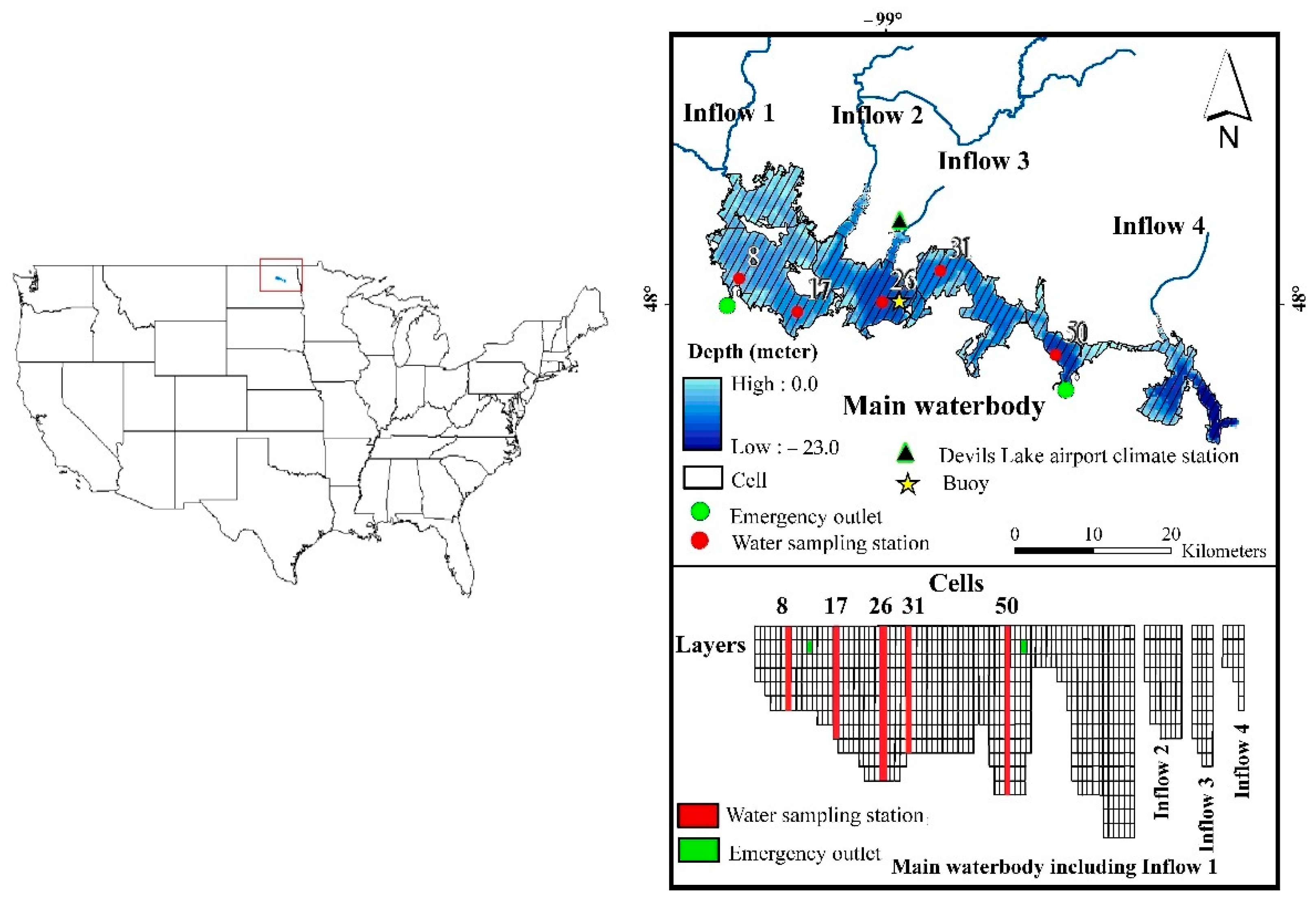
Devils Lake is a terminal lake in Northeast North Dakota (Figure 1) and the largest natural water body in the state. The lake is approximately 80 km long, 1–13 km wide, and relatively shallow, with a maximum water depth of 23 m (Figure 1). Because of inflows from the surrounding farmlands, the lake water is nutrient rich and has low transparency. Devils Lake is well-known for its water-level fluctuations between being dry and overflowing to the Sheyenne River in response to abrupt swing between dry and wet climate cycles [8]. At the current water-surface level of 441 m, the lake encompasses an area of 502 km2 and has a volume of 9829 km3. The climate in Devils Lake is extremely cold in winter and mild in summer, with typical annual temperature ranging from −17 to 27 °C [25]. The average annual precipitation in the area is 518 mm, with the majority of the rainfall occurring in summer [25].
During the study period, 2008–2016, the water temperatures recorded in Devils Lake ranged from −0.25 to 23 °C. Average and maximum wind speeds over the lake were 5 m s−1 and 22 m s−1. Because of its shallow depth and frequent strong wind events, the lake was well mixed during spring, summer, and fall. In the winter season, November to March, the lake was stratified due to having a frozen surface.
2.2. CE-QUAL-W2 Model
CE-QUAL-W2 is a two-dimensional (longitudinal–vertical) hydrodynamic and water-quality model [2]. The model assumes lateral homogeneity in velocities, temperature, and water-quality constituents; therefore, it is best suited for simulating large and narrow waterbodies, such as Devils Lake (Figure 1). The model also includes an ice-cover algorithm, which is important for studying the water quality of Devils Lake in the fall and winter seasons, when the lake surface is frozen.
In configuring the CE-QUAL-W2 model (Figure 1), the lake is divided into 96 cells along approximately west to east direction. Each cell is 1 km long and 1.5 m deep. The number of cells in vertical direction varies depending on the lake bathymetry; the maximum number of layers is 17. The lake has four tributaries, and their daily discharges were simulated by using a Soil and Water Assessment Tool model [11]. The inputs to the CE-QUAL-W2 model, including hourly climate data, such as air temperatures, precipitation, cloud cover, dew point, and wind speeds and directions, were acquired from Automated Surface Observation System Network’s station in Devils Lake (black triangle in Figure 1, [26]). The water temperatures of the tributaries were calculated from air temperatures [27]. Two emergency outlets were defined as being withdrawn in the model, and their daily discharge data were obtained from the North Dakota Water Commission [28]. The model was run to simulate the water temperature of Devils Lake in an hourly time-step. The study period was from 2008 to 2016, with the period from 2008 to 2011 for calibration and from 2012 to 2016 for validation.
Temperature influences physical properties, such as density and salinity, and chemical properties, such as dissolved oxygen and chlorophyll concentrations of a water body. Temperature also affects solubility of oxygen and the rate of photosynthesis, i.e., high temperature increases photosynthesis and reduces solubility of oxygen in water [7]. Six CE-QUAL-W2 parameters listed in Table 1 exert the most influence on simulating water temperature [2,16,17]. Among these parameters, BETA measures the attenuation of solar radiation through water and WSC is used for calculating heat loss, and the rest of the parameters are needed to calculate the heat balance under ice conditions.
2.3. Model Calibration
The CE-QUAL-W2 model was configured to simulate water temperatures of Devils Lake. The objective function for calibrating CE-QUAL-W2 was to minimize the difference between the model-simulated and observed water temperatures. We used profiles of water temperature collected seasonally at five locations in Devils Lake (the red circles and rectangles in Figure 1) to calculate Root Mean Squared Error (RMSE) of simulated water temperatures. In calibration, the values of the model parameters listed in Table 1 were tuned by using IGHS and PSO to minimize the RMSE value of our prediction. We used RMSE as our objective function because it is a standard measure of the CE-QUAL-W2 model performance [6,11,12,16] that can be compared against previous findings. The additional evaluation of the model performance was the coefficient of determination (R2).
2.3.1. HS and IGHS Algorithms
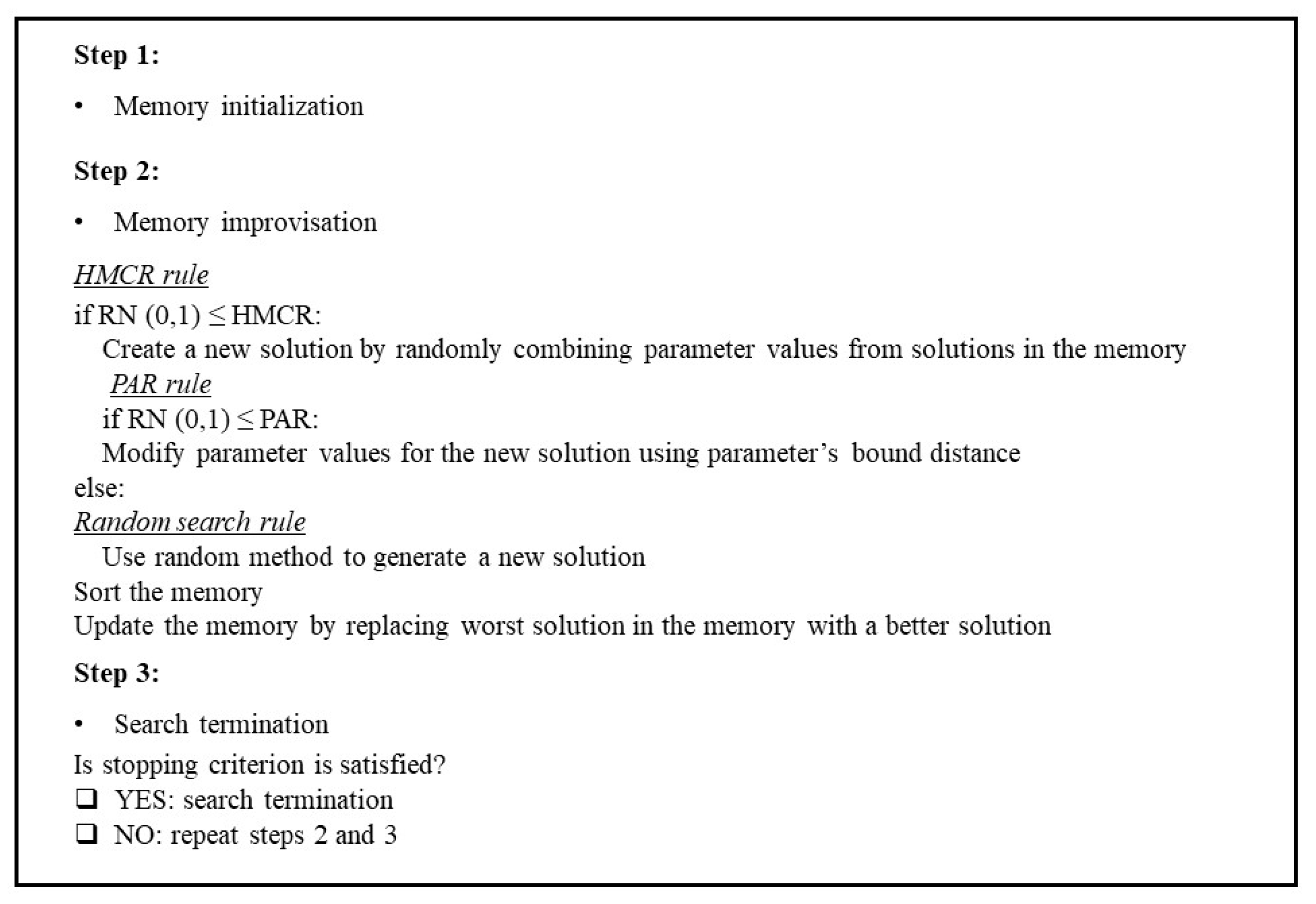
In music, harmony is a pleasing sound created by a group of musical instruments [21]. Inspired by this phenomenon, HS solves the optimization problem by emulating the improvisation process of music players [29]. Generally, HS deploys 3 steps (Figure 2): (1) memory initialization, (2) memory improvisation, and (3) search termination. In the first step, HS initiates the memory (Equations (1) and (2)), using the values of parameters that are randomly selected within their ranges of variation (Equation (3)):
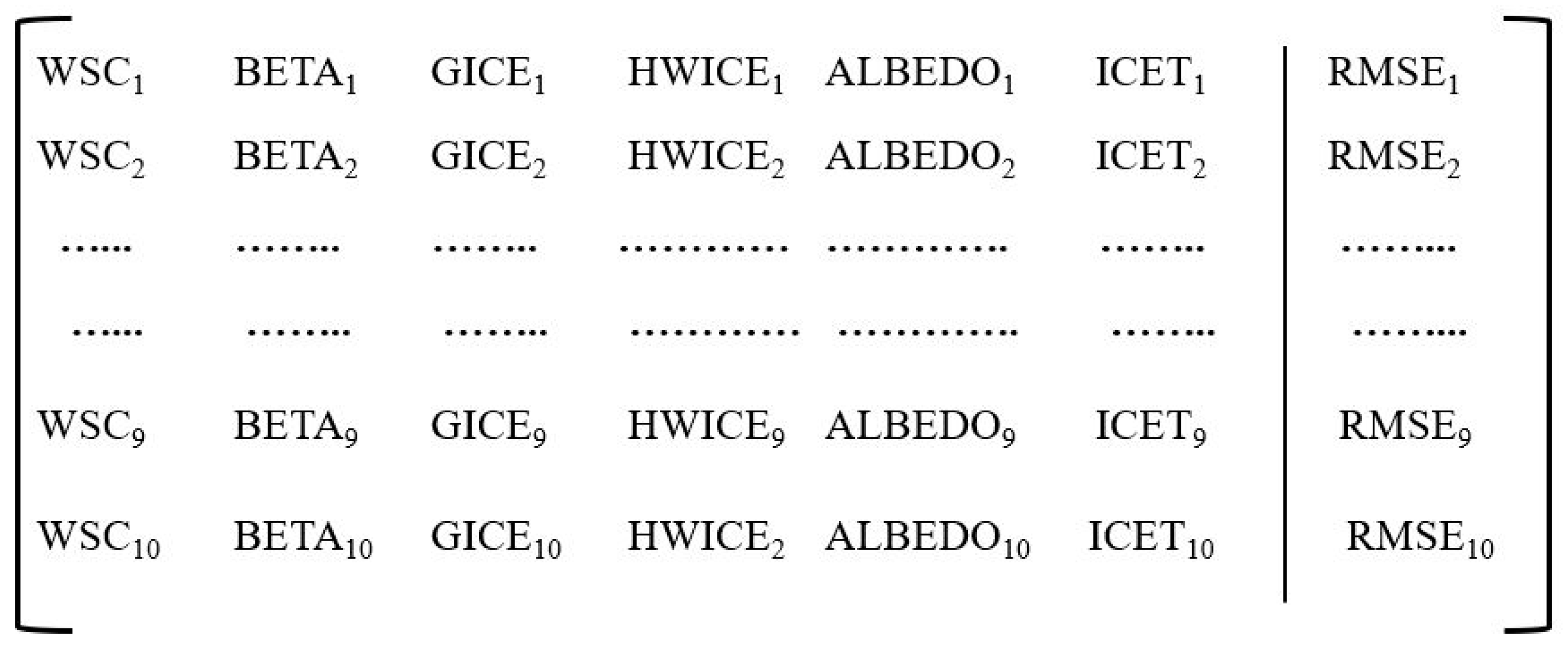
where M is the memory matrix with a total of n solution vectors; Xi represents one solution vector (i = 1 … n), composed of six values (xi,j, j = 1 … 6), representing the six parameters, namely WSC, BETA, GICE, HWICE, ALBEDO, and ICET (Table 1), to be calibrated; xuj and xlj are the upper and lower bounds of the CE-QUAL-W2 parameter, xj; and RN is a random number between 0 and 1.
M = [X1, X2, X3…Xi…, Xn]T
Xi = [xi,1, xi,2, xi,3, …, xi,6]
The second step involves iterations. In each iteration, HS replaces the solution in memory that produces the largest RMSE with a better solution (Figure 2). Two HS parameters are used to regulate the generation of a better solution: Harmony Memory Consideration Rate (HMCR) and Pitch Adjustment Rate (PAR), which typically range from 0.7 to 0.9 and from 0.25 to 0.5, respectively [22]. HMCR determines the contribution of the memory in the improvisation process, and the greater its value is, the greater contribution of the memory. PAR modifies solutions in the memory to prevent a premature convergence of HS [29]. In each iteration, HS creates a random number (RN) between 0 and 1. If RN > HMCR, HS generates a new solution, following Equation (3). If RN ≤ HMCR, then there are two additional steps. First, the HS algorithm generates a new solution (Xnew) by randomly combining parameter values from the existing solutions in the memory (i.e., the HMCR rule). Second, a new RN is generated, and if RN ≤ PAR, the solution will be further modified by using Equation (4) (i.e., the PAR rule):
where is a modified parameter value of the new solution, and is a random number between −1 and 1.
In the third step, HS terminates the search when a predefined criterion is satisfied, which could be a total number of iterations or a specific value for the optimal solution.
The challenge in applying the HS algorithm is to find the proper values for HMCR and PAR, which could be time-consuming [29]. IGHS overcomes this challenge by dynamically tuning the values of HMCR and PAR. Moreover, IGHS improves HS memory initialization and improvisation, which lead to a better global and local search than HS [24].
- IGHS Memory Initialization
Memory initialization is a critical step in HS because a good set of initial solutions can guide the search toward the right direction and potentially lead to a faster convergence. IGHS uses an opposition-based learning method to initiate its memory. In this study, we initialized a memory with 10 solutions (Figure 3) by (1) generating 10 random solutions (Xi, i = 1, …, 10), using Equation (3); (2) calculating their opposite pairs (OXi, i = 1, …, 10, Equation (5)) in the solution space, using Equation (6); and (3) populating the IGHS memory with the 10 solutions that had the smallest RMSEs among the total 20 solutions.
OXi = [oxi,1, oxi,2, oxi,3, ……, oxi,6]
- IGHS Memory Improvisation
Global search (exploration) and local search (exploitation) are defined as the abilities of a metaheuristic algorithm to search different parts and a given part of the solution space to find a solution that is both globally and locally optimal [14]. In HS, HMCR and PAR control global and local search, respectively; that is, a smaller value of HMCR increases global search by promoting random search, and a greater value of HMCR and PAR increases local search by utilizing the memory for search. For HS to converge to an optimal solution, HMCR and PAR values should both increase toward the end of the iterations to prioritize local search [29]. Since periodic functions are typically more suitable for simulating the natural phenomenon [24], IGHS uses a time-varying differential evolution scheme to adjust the values of HMCR and PAR (Equations (7) and (8)):
where HMCRmin, HMCRmax, PARmin, and PARmax represent the lower and upper bounds of HMCR and PAR values, respectively; Iter is the algorithm iteration number; and sgn and sin are sign and sine functions.
In HS, PAR (Equation (4)) conducts a random search and prevents the algorithm from a premature convergence toward a local optimum [24]. IGHS utilizes the best solution in the memory to modify a solution by using a mutation strategy adopted from the differential evolution algorithm based on the PAR rule (Equation (9)):
where best is the index of the best solution in the memory and always equals 1; a and b are unequal random integer numbers between 2 and the size of the memory; and β is an arbitrary scale factor between 0 and 1, which is assumed to be 0.5 here.
Based on the previous finding that random search used in the artificial bee colony algorithm has an advantage in global search [30], IGHS uses Equation (10) [24] for memory improvisation:
where c and d are unequal random integer numbers between 1 and the size of the memory.
In addition to these features, IGHS benefits from two perturbation schemes to further enhance its exploration by modifying the best solution in the memory during random iterations [24]. Since these perturbation schemes could reduce the convergence speed of IGHS [24], we did not use them in this study. We arbitrarily terminated the IGHS algorithm after 50 iterations.
2.3.2. PSO Algorithm
PSO is a metaheuristic algorithm derived from animal social behaviors [23]. The algorithm is inspired by the swarm behavior of a group of animals, such as fish and birds, searching for food and shelter. Similar to IGHS, PSO is a memory-based algorithm with 3 steps: (1) solutions initialization, (2) solutions movement, and (3) search termination [23].
PSO searches the solution space for an optimal solution by moving a group of candidate solutions toward the best solution in the memory (local optimum). The algorithm uses velocity vectors to move solutions in the solution space. PSO generates a velocity vector for a solution by using the parameters information from (1) the local optimum and (2) the best model output that is so far achieved by the solution. PSO uses the group and individual information to calculate the velocities of solutions. The algorithm stores parameter values for the local optimum and the best output achieved by the solutions to separate memories and updates them at the end of each iteration. To use PSO for calibration of CE-QUAL-W2, we used Equation (3) to generate 10 random solutions (X1, …, X10). We then created the initial vector of velocities (v) for 10 initial PSO solutions by generating the velocity for their parameter values:
In each iteration, the velocity of each solution was updated by using Equations (12)–(14):
where is the new velocity; xPbest is a parameter value used in simulating the best CE-QUAL-W2 output so far; xGbest is the value of the parameter from a local optimum; w is the inertia weight; w1 and w2 are the maximum and minimum values of inertia weight and are equal to 0.9 and 0.4, respectively; and c1 and c2 are acceleration constants and are equal to 0.5 [16]. Since PSO in each iteration generates 10 new solutions, for a fair comparison with IGHS, we ran PSO for 5 iterations, resulting in a total of 50 runs for calibrating the CE-QUAL-W2 model by using IGHS.
2.4. Model Validation
To validate the CE-QUAL-W2 model calibrated by IGHS and PSO algorithms, we compared simulated water temperatures against observations for the period from 2011 to 2016. Over the same period, we have deployed a buoy in Devils Lake (yellow star in Figure 1) during the non-freezing seasons to collect various water-quality-related data, including the water temperature at a depth of ~0.5 m. We averaged the temperature data collected every 10 min into hourly values for validation. We used RMSE and R2 to evaluate the validation results.
2.5. Uncertainty of Automatic Calibration
The uncertainty of automatic calibration was estimated by using the final ten values of the model parameters that are in the memory, assuming that they represent optimal range of parameter values [31,32,33]. Specifically, we used the range of model outputs corresponding to the final solutions in the memory to represent the uncertainty of calibration. We also increased the number of CE-QUAL-W2 runs from 50 to 100 to test sensitivity of our simulation results.
3. Results
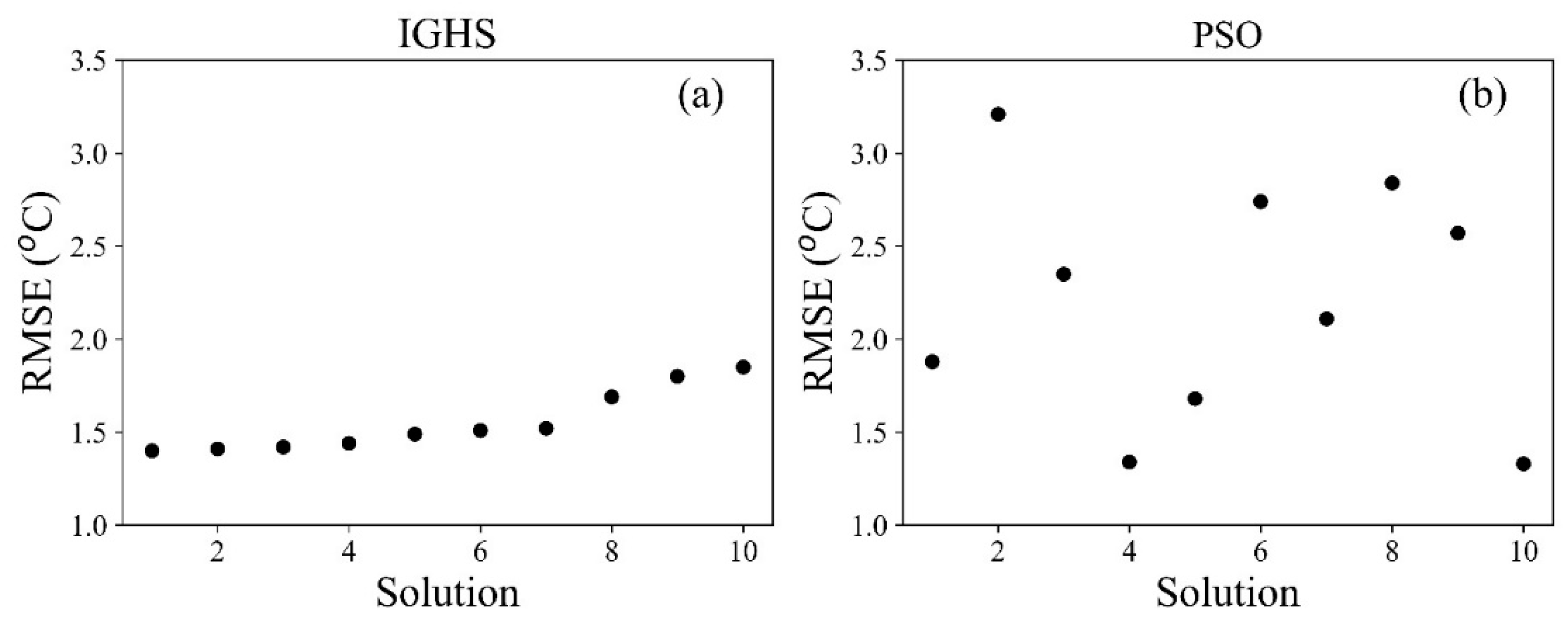
The initial memories generated for IGHS and PSO are presented in Figure 4. The RMSE values of the initial solutions range from 1.4 to 1.8 °C for IGHS (Figure 4a) and 1.33 to 3.21 °C for PSO (Figure 4b). Though the PSO has a solution with the smallest RMSE (1.33 °C), the IGHS solutions are more robust, with a median RMSE value of 1.5 °C, compared to the 2.3 °C for PSO. This indicates that the opposition-based learning method used in IGHS can produce better-fitted solutions to fill the memory than the random search used in PSO.
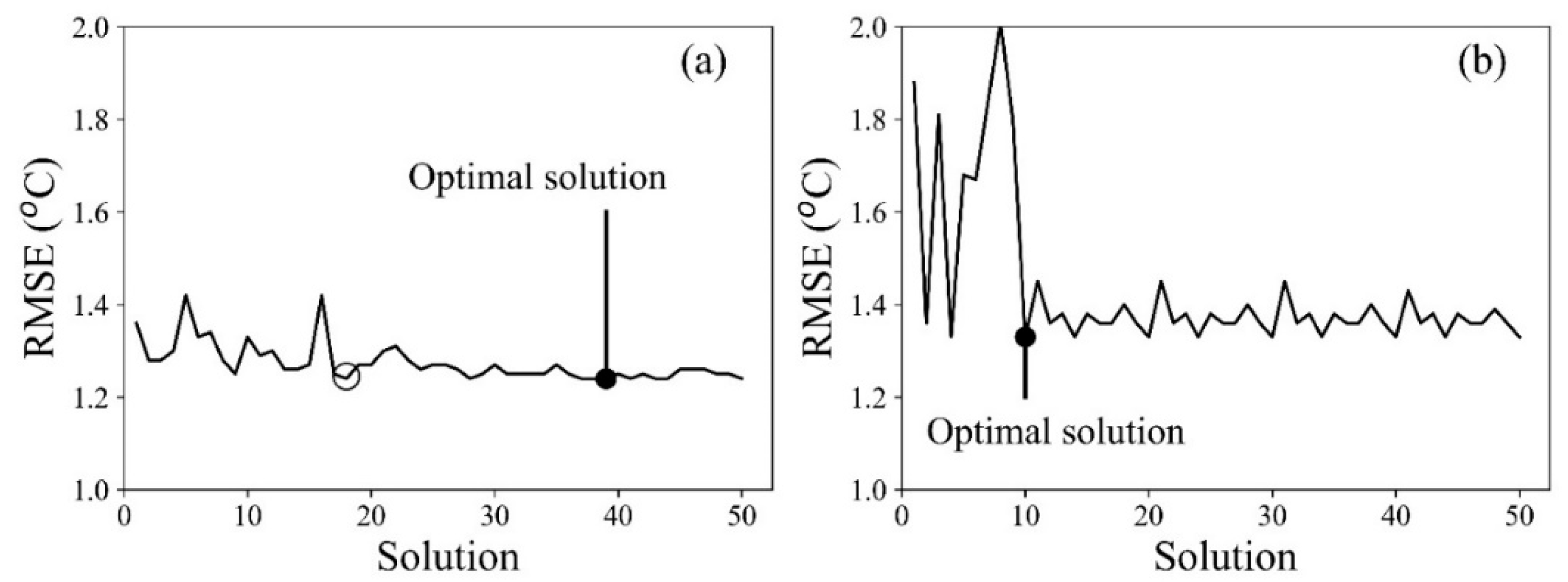
Figure 5a shows how the IGHS algorithm converged to the final solution during calibration. Based on the variations of RMSE values over the 50 iterations, we found that the IGHS algorithm went through two phases of the search. During the first 20 iterations, where variations in the RMSE values were relatively greater, the algorithm conducted global search or explored the solution space. This is because IGHS started with a small value of HMCR, which favors exploration (i.e., global search). In addition, the diversity of parameter values in initial solutions helped to enforce this global search when IGHS used the memory for the improvisation process. As a result of this global search, IGHS found a new optimal solution with RMSE = 1.24 °C in iteration 18 (open dot in Figure 5a).
With the number of iterations and the HMCR value increasing, IGHS was directed to use more memory for its search following the HMCR and PAR rules, and hence the RMSE values varied relatively less after entering the second phase of the search. Through the local search (or exploitation), IGHS was able to update the previous optimal solution that was identified in iteration 18 with a new optimal solution that has RMSE = 1.23 °C in iteration 39 (filled dot in Figure 5a). Later iterations did not result in a better solution, and IGHS converged by suggesting this solution as the optimal solution for calibrating the CE-QUAL-W2 model.
The convergence of the PSO algorithm for calibrating CE-QUAL-W2 is presented in Figure 5b. During the first 10 iterations, PSO explored the solution space by updating solutions in the memory and found an optimum solution at iteration 10 (filled dot in Figure 5b) with RMSE = 1.33 °C. In the following iterations, PSO updated the solutions’ velocity by using the parameter information from the local optimum (solution number 10) and the best model output for individual solutions. Despite this effort, the algorithm failed to identify a better solution than the one generated during the memory initialization step. This indicates that PSO was trapped in a local optimum through the entire course of CE-QUAL-W2 calibration (Figure 5b).
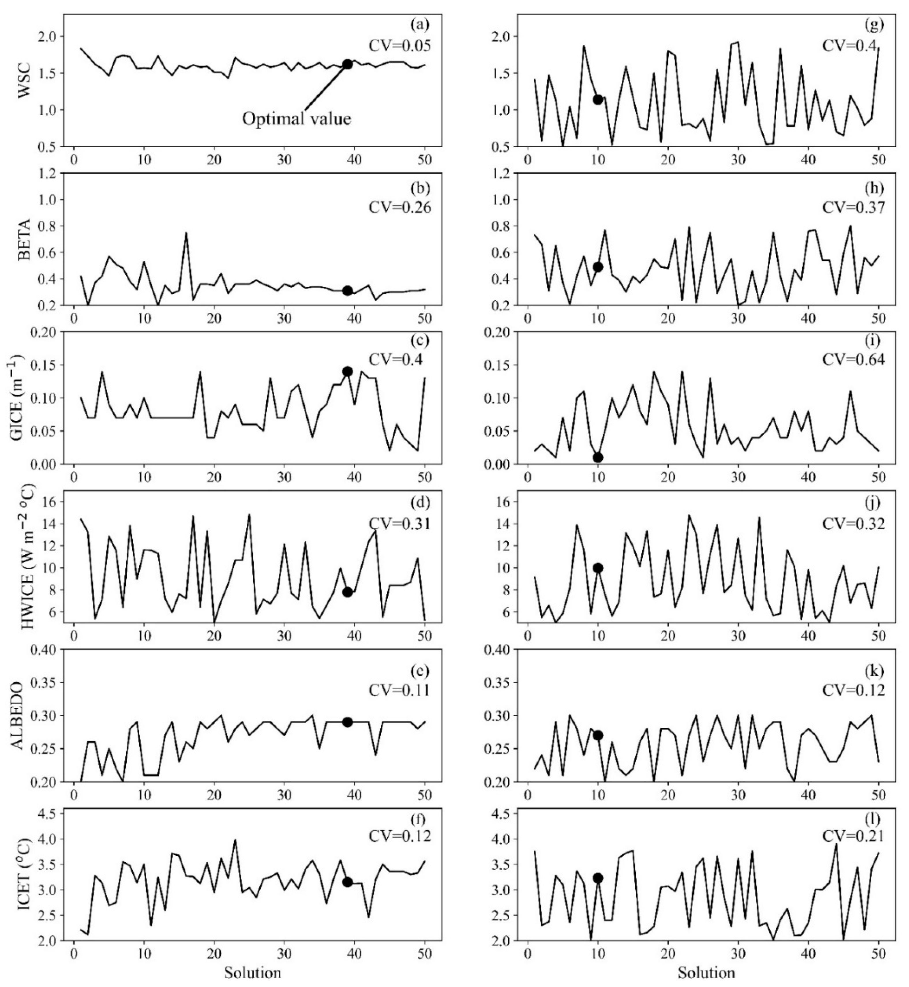
The run-time values of the CE-QUAL-W2 parameters and their optimal values contained in IGHS and PSO solutions are presented in Figure 6, which shows that the parameter values generated by both IGHS and PSO were within their specified ranges (Table 1). Overall, there is a greater variation (CV) in the parameter values among PSO solutions than those among IGHS solutions, which in turn leads to the larger variation in RMSE values observed for PSO algorithm (Figure 5). Examining the variations of the six parameters during the IGHS calibration indicated that the calibration was mainly driven by the convergence of WSC and BETA (Figure 6a,b).
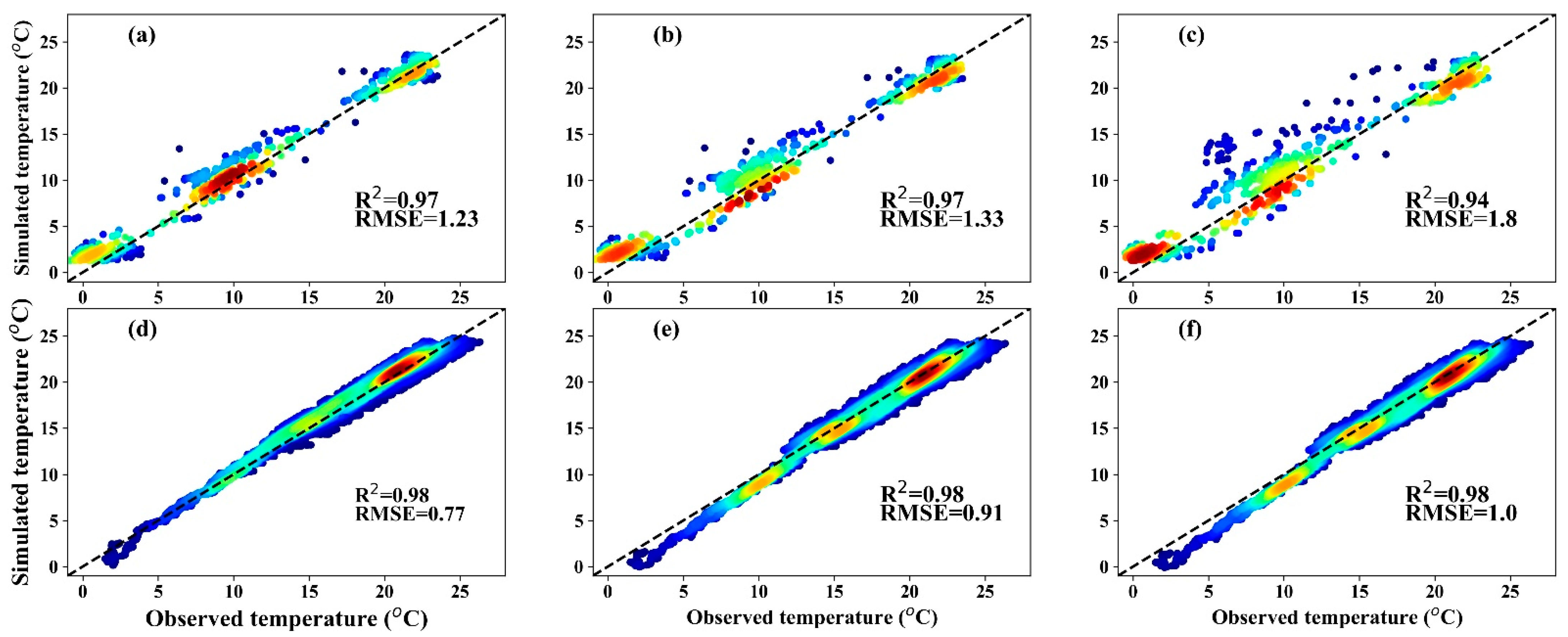
The performance of automatic calibration was further examined against the manual calibration for both calibration and validation periods (Table 2 and Figure 7). For calibration, the CE-QUAL-W2 model simulated water temperatures with R2 = 0.97, and RMSE = 1.23 and 1.33 °C for IGHS and PSO, respectively (Figure 7a,b). For validation, the calibrated model resulted in R2 = 0.98, and RMSE = 0.77 and 0.91 °C for IGHS and PSO, respectively (Figure 7d,e). Compared to manual calibration (Figure 7c,f), automatic calibration using either IGHS or PSO resulted in a better performance of the model. Among the three calibration methods, the CE-QUAL-W2 model calibrated by IGHS performed the best in simulating water temperatures of Devils Lake for both calibration and validation periods with the smallest RMSE values.
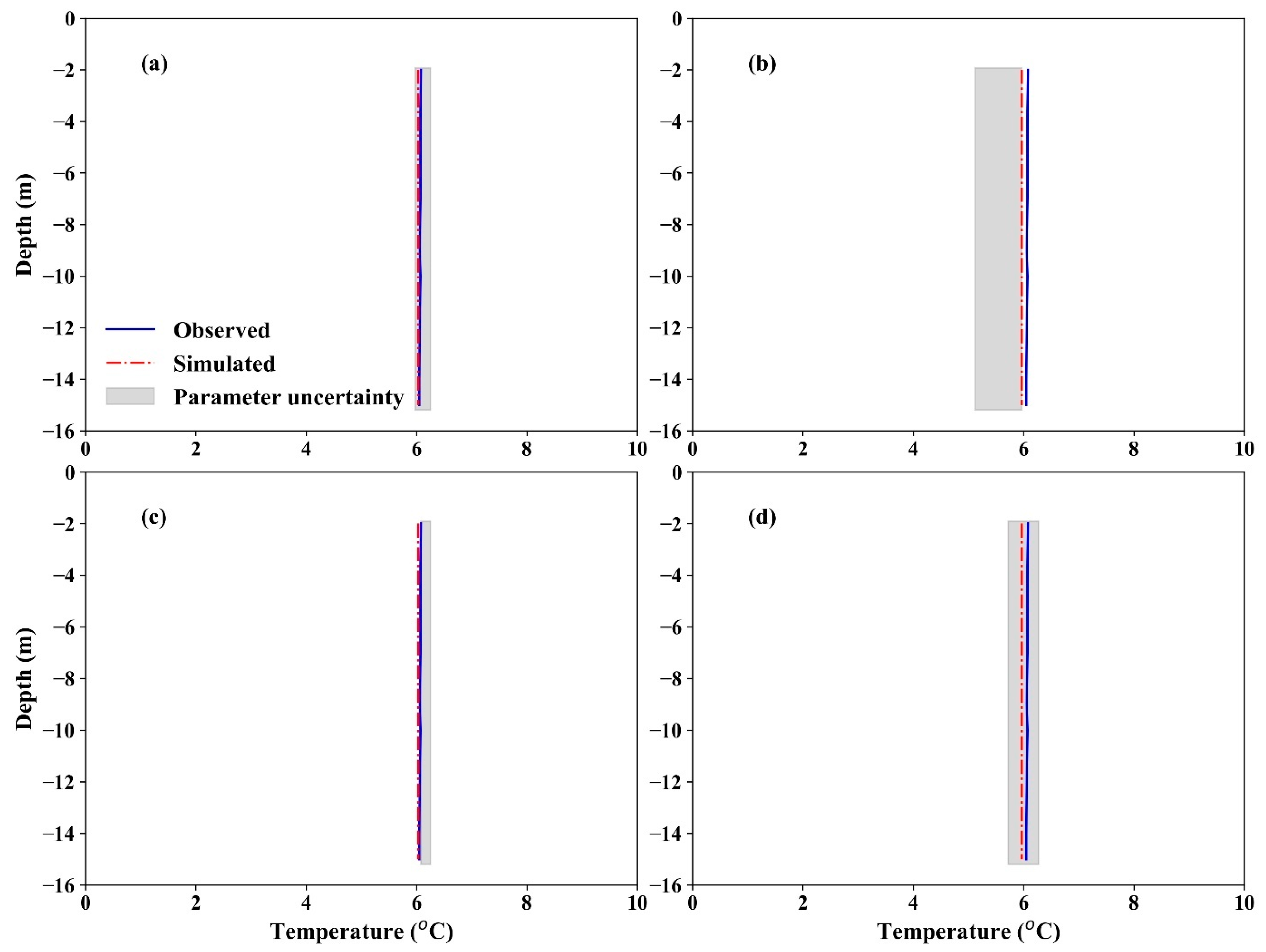
The uncertainty of the calibration was estimated by using the final 10 values of the model parameters that were in the memory. For illustration, we showed the final 10 water-temperature profiles simulated for segment 50 on 4 November 2009 (Figure 8), with the calibration-chosen output shown as red and the range of final 10 outputs as the shaded area. For comparison, we also showed the observed temperature (blue). Both calibrations were able to reproduce the distribution of water temperature (which was rather uniform), but the model calibrated by IGHS (Figure 8a) performed better than PSO (Figure 8b), with the average difference between modeled and observed temperature being 0.04 °C vs. 0.11 °C. The uncertainty of IGHS calibration was also better constrained than PSO; the ranges of shaded area are 0.26 and 0.85 °C for IGHS and PSO, respectively. Increasing the number of the model runs in calibration from 50 to 100 did decrease the uncertainty of PSO calibration to 0.55 (Figure 8d) but barely affected the IGHS calibration (Figure 8c). However, we did not observe improvement in accuracy of simulated water temperatures with increased iteration numbers in calibration.
4. Discussion
Global search and local search are two main features of metaheuristic algorithms that determine their capabilities in solving optimization problems [14]. In our study, IGHS and PSO started their searches by exploring the solution space and converged by exploiting parts of the solution space that were detected as the potential location for the global optimum (Figure 5). PSO is well-known for its global search [13]. As expected, PSO carried out a wider global search than IGHS (Figure 5). However, PSO was trapped in a local optimum that was detected during the initialization of memory, resulting a solution with RMSE = 1.33 °C (Figure 5b). This happened because (1) PSO failed to find a better global optimum during its exploration, and (2) the inefficient local search prevented PSO from detecting a better local optimum in the given solution space.
A small number of applied iterations (five iterations) is one of the main reasons for the PSO’s inefficient local search. In PSO, global search and local search were controlled by the velocity of solutions, and the velocity decreases linearly with iterations. Since a smaller velocity created greater exploitation, using only a small number of iterations prevented the algorithm from carrying out a comprehensive local search. We used a small number of iterations for calibration because CE-QUAL-W2 is a computationally intensive program and the model uses only one unit of the computer’s Central Process Unit (CPU) for its calculation [12]. For our study, each CE-QUAL-W2 run took ~30 min, and the entire calibration (50 runs) lasted 25 h. However, by using the same number of the model runs, IGHS still effectively explored the solution space and identified a near-global optimum, with RMSE = 1.24 °C, in iteration 18. By exploiting the part of the solution space around this optimum, the algorithm found a global optimum with RMSE = 1.23 °C in iteration 39.
Among the six CE-QUAL-W2 parameters that were calibrated, WSC and BETA are the most sensitive parameters in simulating water temperature in Devils Lake [11]. The run-time variation of the six parameters during the calibration (Figure 6) showed that WSC and BETA converged in IGHS (Figure 6a,b) but not in PSO (Figure 6g,h), suggesting that IGHS was able to capture the sensitivity of the parameters in model calibration.
We used RMSE and R2 to perform an end-of-run comparative analysis between the two metaheuristic algorithms [14]. Based on these two statistic parameters estimated for both calibration and validation periods, the CE-QUAL-W2 model calibrated by IGHS produced a better simulation compared to PSO (Table 2 and Figure 7), and the difference in performance between the two calibration algorithms is statistically significant. For instance, we estimated that the mean and standard deviation of the difference between simulated and observed water temperature during validation period are 0.6 and 0.4 °C for IGHS and 0.8 and 0.5 °C for PSO, respectively. A t-test showed that these differences between the two algorithms are statistically significant (p < 0.01). In summary, we found that using the IGHS algorithm for calibration leads to statistically significant improvement in the performance of CE-QUAL-W2, at least in our case of simulating water temperature. Moreover, the performance of our IGHS-calibrated CE-QUAL-W2 is comparable to the other studies that have used CE-QUAL-W2 to simulate water temperature (Table 3).
Despite the advantages of metaheuristic algorithms, namely IGHS and PSO, for the calibration of the CE-QUAL-W2 model, there is uncertainty associated with their applications, due to the stochastic nature of the calibration process and the constraint in computation resource [14]. Therefore, the solutions generated from these empirical algorithms inherited such uncertainty. We further assessed the uncertainties associated with IGHS and PSO by increasing the number of model iterations (Figure 8c,d). We found that the uncertainty in PSO calibration was reduced significantly when the length of calibration was increased from 50 to 100 model runs (Figure 8d), but the change was negligible for IGHS (Figure 8c).
It should be noted that the calibration of CE-QUAL-W2 in this study was an optimization problem with a single objective function and non-linear constraints. Future research should explore and validate the advantages of using IGHS to calibrate CE-QUAL-W2 model with multi-objectives and multicriteria problems, such as simulating water temperature, dissolved oxygen, and chlorophyll concentration simultaneously. This will help to evaluate the full capability of the IGHS algorithm for calibrating the CE-QUAL-W2 model in solving more complex water-quality problems.
Our IGHS calibration framework optimizes the model parameters to increase accuracy and reduce uncertainty in the model prediction. By quantifying parameter uncertainty, our program partially calculates the uncertainty of the model output. One potential route for future research can involve integrating the calibration framework with an uncertainty model to propagate uncertainty associated with model inputs and structure on CE-QUAL-W2 output.
5. Conclusions
CE-QUAL-W2 calibration can be a challenging task due to the complex behavior of water-quality constituents in the environment and the non-linear behavior of the model’s parameters. By testing two metaheuristic algorithms, namely IGHS and PSO, for automatic calibration of CE-QUAL-W2, we found that the IGHS could overcome these challenges and create reliable and robust calibration for simulating water temperature. The IGHS-calibrated model could simulate the vertical and temporal variations of the Devils Lake water temperatures with RMSE = 1.23 and 0.77 °C for the calibration and validation periods (Figure 7a,d). For comparison, the corresponding RMSEs for PSO-calibrated model are 1.33 and 0.91 °C, respectively. Measured by RMSE, the model performance improved by 7–15% with IGHS calibration as compared to PSO calibration. Both automatically calibrated models performed better than manually calibrated model.
Because CE-QUAL-W2 only uses one CPU unit for numerical computations, its calibration is a time-consuming process. This makes exploration of the entire solution space almost unfeasible, and as a result, we had to limit the global search of PSO and IGHS to a small number of iterations. To solve this computationally intensive optimization problem, where the chance of finding the global solution through global search is limited, we found that, by wisely using the control parameters, IGHS resulted in better calibration than PSO. This is because IGHS was able to identify the most sensitive parameters, BETA and WSC, through its global search and converge quickly to their optimal values during its local search. The method developed in this study is also applicable for simulating other water-quality constituents in Devils Lake or water bodies in different regions to improve the performance and efficiency in model calibration.
Author Contributions
A.S. and X.Z. designed the research. A.S. performed the analysis and drafted the manuscript. X.Z., H.Z. and X.C. provided advice during the research and helped to revise the paper. All authors have read and agreed to the published version of the manuscript.
Funding
This work was supported by National Science Foundation under grant 1355466, USDA under grant 2013-67010-21358, and North Dakota Water Resources Research Institute 2017–2018 Fellowship.
Institutional Review Board Statement
Not applicable.
Informed Consent Statement
Not applicable.
Data Availability Statement
The Python code developed in this research is available upon reasonable request.
Conflicts of Interest
The authors declare no conflict of interest.
References
- Flowers, J.D.; Hauck, L.M.; Kiesling, R.L. USDA: Lake Waco-Bosque River Initiative Water Quality Modeling of Lake Waco Using CE-QUAL-W2 for Assessment of Phosphorus Control Strategies; Texas Institute for Applied Environmental Research: Stephenville, TX, USA, 2001; p. 76. [Google Scholar]
- Cole, T.M.; Wells, S.A. CE-QUAL-W2: A Two-Dimensional, Laterally Averaged, Hydrodynamic and Water Quality Model, Version 3.1; US Army Engineering and Research Development Center: Vicksburg, MS, USA, 2003; p. 630. [Google Scholar]
- Debele, B.; Srinivasan, R.; Parlange, J.Y. Coupling upland watershed and downstream waterbody hydrodynamic and water quality models (SWAT and CE-QUAL-W2) for better water resources management in complex river basins. Environ. Modeling Assess. 2008, 13, 135–153. [Google Scholar] [CrossRef]
- Bowen, J.D.; Harrigan, N.B. Water Quality Model Calibration via a Full-Factorial Analysis of Algal Growth Kinetic Parameters. J. Mar. Sci. Eng. 2018, 6, 137. [Google Scholar] [CrossRef] [Green Version]
- Lindenschmidt, K.-E.; Carr, M.K.; Sadeghian, A.; Morales-Marin, L. CE-QUAL-W2 model of dam outflow elevation impact on temperature, dissolved oxygen and nutrients in a reservoir. Sci. Data 2019, 6, 312. [Google Scholar] [CrossRef]
- Kim, Y.; Kim, B. Application of a 2-Dimensional Water Quality Model (CE-QUAL-W2) to the Turbidity Interflow in a Deep Reservoir (Lake Soyang, Korea). Lake Reserv. Manag. 2006, 22, 213–222. [Google Scholar] [CrossRef]
- Noori, R.; Berndtsson, R.; Franklin Adamowski, J.; Rabiee Abyaneh, M. Temporal and depth variation of water quality due to thermal stratification in Karkheh Reservoir, Iran. J. Hydrol. Reg. Stud. 2018, 19, 279–286. [Google Scholar] [CrossRef]
- Shabani, A.; Zhang, X.; Chu, X.; Dodd, T.P.; Zheng, H. Mitigating Impact of Devils Lake Flooding on the Sheyenne River Sulfate Concentration. J. Am. Water Resour. Assoc. 2020, 56, 297–309. [Google Scholar] [CrossRef]
- Noori, R.; Tian, F.; Ni, G.; Bhattarai, R.; Hooshyaripor, F.; Klöve, B. ThSSim: A novel tool for simulation of reservoir thermal stratification. Sci. Rep. 2019, 9, 18524. [Google Scholar] [CrossRef] [Green Version]
- Buccola, N.L.; Stonewall, A.J. Development of a CE-QUAL-W2 Temperature Model for Crystal Springs Lake, Portland, Oregon; Open-File Report 2016–1076; United States Geological Survey: Reston, VA, USA, 2016. [Google Scholar]
- Shabani, A.; Zhang, X.; Ell, M. Modeling Water Quantity and Sulfate Concentrations in the Devils Lake Watershed Using Coupled SWAT and CE-QUAL-W2. J. Am. Water Resour. Assoc. 2017, 53, 748–760. [Google Scholar] [CrossRef]
- Afshar, A.; Shojaei, N.; Sagharjooghifarahani, M. Multiobjective Calibration of Reservoir Water Quality Modeling Using Multiobjective Particle Swarm Optimization (MOPSO). Water Resour. Manag. 2013, 27, 1931–1947. [Google Scholar] [CrossRef]
- Tayfur, G. Modern Optimization Methods in Water Resources Planning, Engineering and Management. Water Resour. Manag. 2017, 31, 3205–3233. [Google Scholar] [CrossRef]
- Maier, H.R.; Kapelan, Z.; Kasprzyk, J.; Kollat, J.; Matott, L.S.; Cunha, M.C.; Dandy, G.C.; Gibbs, M.S.; Keedwell, E.; Marchi, A.; et al. Evolutionary algorithms and other metaheuristics in water resources: Current status, research challenges and future directions. Environ. Model. Softw. 2014, 62, 271–299. [Google Scholar] [CrossRef] [Green Version]
- Yoo, D.G.; Kim, J.H. Meta-heuristic algorithms as tools for hydrological science. Geosci. Lett. 2014, 1, 4. [Google Scholar] [CrossRef] [Green Version]
- Afshar, A.; Kazemi, H.; Saadatpour, M. Particle Swarm Optimization for Automatic Calibration of Large Scale Water Quality Model (CE-QUAL-W2): Application to Karkheh Reservoir, Iran. Water Resour. Manag. 2011, 25, 2613–2632. [Google Scholar] [CrossRef]
- Ostfeld, A.; Salomons, S. A hybrid genetic—Instance based learning algorithm for CE-QUAL-W2 calibration. J. Hydrol. 2005, 310, 122–142. [Google Scholar] [CrossRef]
- Chen, Y.; Li, J.; Xu, H. Improving flood forecasting capability of physically based distributed hydrological models by parameter optimization. Hydrol. Earth Syst. Sci. 2016, 20, 375–392. [Google Scholar] [CrossRef] [Green Version]
- Kazemi, H. Calibration of Large Scale Water Quality Model (CE-QUAL-W2) by Hybrid Algorithm. Master’s Thesis, Iran University of Science and Technology, Tehran, Iran, 2010. [Google Scholar]
- Evers, G.I.; Ghalia, M.B. Regrouping particle swarm optimization: A new global optimization algorithm with improved performance consistency across benchmarks. In Proceedings of the 2009 IEEE International Conference on Systems, Man and Cybernetics, San Antonio, TX, USA, 11–14 October 2009; pp. 3901–3908. [Google Scholar]
- Zong Woo, G.; Joong Hoon, K.; Loganathan, G.V. A New Heuristic Optimization Algorithm: Harmony Search. Simulation 2001, 76, 60–68. [Google Scholar] [CrossRef]
- Ayvaz, M.T. Solution of Groundwater Management Problems Using Harmony Search Algorithm. In Recent Advances in Harmony Search Algorithm; Geem, Z.W., Ed.; Springer: Berlin/Heidelberg, Germany, 2010; Volume 270. [Google Scholar]
- Karahan, H.; Gurarslan, G.; Geem Zong, W. Parameter Estimation of the Nonlinear Muskingum Flood-Routing Model Using a Hybrid Harmony Search Algorithm. J. Hydrol. Eng. 2013, 18, 352–360. [Google Scholar] [CrossRef]
- Xiang, W.; An, M.; Li, Y.; He, R.; Zhang, J. An improved global-best harmony search algorithm for faster optimization. Expert Syst. Appl. 2014, 41, 5788–5803. [Google Scholar] [CrossRef]
- Hoerling, M.; Eischeid, J.; Easterling, D.; Peterson, T.; Webb, R. Understanding and Explaining Hydro-Climate Variation at Devils Lake; National Oceanic and Atmospheric Administration: Washington, DC, USA, 2010; pp. 1–21. [Google Scholar]
- Automated Surface Observing Systems. Hourly Climate Data. Available online: https://www.weather.gov/asos/asostech (accessed on 1 August 2018).
- Neitsch, S.L.; Arnold, J.G.; Williams, J.R. Soil and Water Assessment Tool Theorethical Documentation Version 2009; Texas Water Resource Institute: College Station, TX, USA, 2009; p. 647. [Google Scholar]
- The North Dakota State Water Commission. Devils Lake Outlets Discharge Monitoring Reports. Available online: https://www.swc.nd.gov/basins/devils_lake/outlets/ (accessed on 1 August 2018).
- Mahdavi, M.; Fesanghary, M.; Damangir, E. An improved harmony search algorithm for solving optimization problems. Appl. Math. Comput. 2007, 188, 1567–1579. [Google Scholar] [CrossRef]
- Karaboga, D.; Basturk, B. A powerful and efficient algorithm for numerical function optimization: Artificial bee colony (ABC) algorithm. J. Global Optim. 2007, 39, 459–471. [Google Scholar] [CrossRef]
- Abbaspour, K.C. SWAT-CUP 2012: SWAT Calibration and Uncertainty Programs—A User Manual; Swiss Federal Institute of Aquatic Science and Technology: Zürich, Switzerland, 2014; p. 106. [Google Scholar]
- Abbaspour, K.C.; Rouholahnejad, E.; Vaghefi, S.; Srinivasan, R.; Yang, H.; Kløve, B. A continental-scale hydrology and water quality model for Europe: Calibration and uncertainty of a high-resolution large-scale SWAT model. J. Hydrol. 2015, 524, 733–752. [Google Scholar] [CrossRef] [Green Version]
- Abbaspour, K.C.; Yang, J.; Maximov, I.; Siber, R.; Bogner, K.; Mieleitner, J.; Zobrist, J.; Srinivasan, R. Modelling hydrology and water quality in the pre-alpine/alpine Thur watershed using SWAT. J. Hydrol. 2007, 333, 413–430. [Google Scholar] [CrossRef]
- Shojaei, N. Automatic Calibration of Water Quality Model and Hydrodynamic Model (CE-QUAL-W2); Portland State University: Portland, OR, USA, 2014. [Google Scholar]
- Noori, R.; Asadi, N.; Deng, Z. A simple model for simulation of reservoir stratification. J. Hydraul. Res. 2019, 57, 561–572. [Google Scholar] [CrossRef]
- United States Army Corps of Engineer. Application and Calibration of the CE-QUAL-W2 Version 3.71 Hydrodynamic and Water Quality Model for Zorinsky Reservoir; USACE: Omaha, NE, USA, 2015; pp. 1–171.
Figure 1.
Map of Devils Lake and its discretization in the CE-QUAL-W2 model [17]. The five red points and rectangles represent the locations for seasonal water-temperature sampling. The two green circles and rectangles represent the two emergency outlets. The black triangle represents the location of a weather station, and the yellow star represents the location of the buoy in 2015.

Figure 2.
General structure of Harmony Search (HS) algorithm. Harmony Memory Consideration Rate (HMCR) and Pitch Adjustment Rate (PAR) are control parameters used in HS.
Figure 2.
General structure of Harmony Search (HS) algorithm. Harmony Memory Consideration Rate (HMCR) and Pitch Adjustment Rate (PAR) are control parameters used in HS.

Figure 3.
Scheme of the IGHS memory applied for calibration of CE-QUAL-W2 model. Each row in this schematic memory represents a solution which is composed of six CE-QUAL-W2 parameters and a corresponding RMSE value calculated by comparing model-simulated temperatures with observations.
Figure 3.
Scheme of the IGHS memory applied for calibration of CE-QUAL-W2 model. Each row in this schematic memory represents a solution which is composed of six CE-QUAL-W2 parameters and a corresponding RMSE value calculated by comparing model-simulated temperatures with observations.

Figure 4.
(a) IGHS initial memory generated by the opposition-based learning method, and (b) PSO initial memory generated by using random search.
Figure 4.
(a) IGHS initial memory generated by the opposition-based learning method, and (b) PSO initial memory generated by using random search.

Figure 5.
(a) IGHS solutions and (b) PSO solutions generated through 50 iterations for calibration of CE-QUAL-W2 model. Black open and filled dots represent the local and global optimum solutions.
Figure 5.
(a) IGHS solutions and (b) PSO solutions generated through 50 iterations for calibration of CE-QUAL-W2 model. Black open and filled dots represent the local and global optimum solutions.

Figure 6.
(a–f) Left panel and (g–l) right panel show the CE-QUAL-W2 parameter values for IGHS and PSO solutions, respectively. Black dots show the optimal values for the CE-QUAL-W2 parameters. CV is the coefficient of variation, and its higher value means larger variation from the calculated mean.
Figure 6.
(a–f) Left panel and (g–l) right panel show the CE-QUAL-W2 parameter values for IGHS and PSO solutions, respectively. Black dots show the optimal values for the CE-QUAL-W2 parameters. CV is the coefficient of variation, and its higher value means larger variation from the calculated mean.

Figure 7.
Comparison of Devils Lake water temperatures between simulation and observation. (a–c) Simulated by CE-QUAL-W2 model that was calibrated by using IGHS, PSO, and manual [11] methods, respectively, during the calibration period. (d–f) Same as (a–c) but for validation period. Dark blue and red colors represent low and high density of water temperature data.

Figure 8.
Observed (red) and simulated (blue) water-temperature profiles for segment 50 on 4 November 2009. The shaded areas represent the ranges of temperature simulated by using the final 10 parameter values that were in memory. (a,b) Calibration with 50 runs by IGHS and PSO, respectively; (c,d) same as (a,b) but with 100 runs in calibration.


Table 1.
The six CE-QUAL-W2 parameters and the ranges of their values that are calibrated for simulating water temperature in Devils Lake.
Table 1.
The six CE-QUAL-W2 parameters and the ranges of their values that are calibrated for simulating water temperature in Devils Lake.
| CE-QUAL-W2 Model Parameters | Name | Default Values | Feasible Ranges [3] |
|---|---|---|---|
| Wind sheltering coefficient | WSC | 1.0 | 0.5–2.0 |
| Fraction of solar radiation absorbed within 0.6 m depth of water | BETA | 0.45 | 0.20–0.8 |
| Solar radiation extinction coefficient (m−1) | GICE | 0.07 | 0.01–0.14 |
| Coefficient of water–ice heat exchange through the melt layer (W m−2 °C) | HWICE | 10.0 | 5.0–15.0 |
| Fraction of solar radiation reflected by the ice surface | ALBEDO | 0.25 | 0.20–0.30 |
| Temperature above which ice formation is not allowed (°C) | ICET | 3.0 | 2.0–4.0 |
Table 2.
The optimal values of the six CE-QUAL-W2 parameters calibrated by IGHS, PSO, and manually, and the calculated RMSE values of the simulated Devils Lake water temperatures for both calibration and validation periods.
Table 2.
The optimal values of the six CE-QUAL-W2 parameters calibrated by IGHS, PSO, and manually, and the calculated RMSE values of the simulated Devils Lake water temperatures for both calibration and validation periods.
| Calibration Method | CE-QUAL-W2 Parameter Value | RMSE (°C) | ||||||
|---|---|---|---|---|---|---|---|---|
| WSC | BETA | GICE | HWICE | ALBEDO | ICET | Calibration | Validation | |
| IGHS | 1.62 | 0.31 | 0.14 | 7.79 | 0.29 | 3.15 | 1.23 | 0.77 |
| PSO | 1.14 | 0.49 | 0.01 | 9.98 | 0.27 | 3.23 | 1.33 | 0.91 |
| Manual | 2.0 | 0.7 | – | – | – | – | 1.8 | 1.0 |
Table 3.
Performance comparison of CE-QUAL-W2 simulation of water temperature between this study and previous studies.
Table 3.
Performance comparison of CE-QUAL-W2 simulation of water temperature between this study and previous studies.
| Study Location | Simulation Length | Metric | Error (°C) |
|---|---|---|---|
| Devils Lake, USA (This study) | 8 years (2008–2016) | RMSE | 0.7–1.23 |
| Lake Soyang, South Korea [6] | 7 years (1995–2002) | RMSE | 1.93 |
| Karkheh Dam Reservoir, Iran [34] | One year (2005) | RMSE | 0.8 |
| Karkheh Dam Reservoir, Iran [35] | ---- | MAE | 0.67–0.71 |
| Crystal Spring Lake, USA [10] | One year (2014) | MAE | 0.2–0.6 |
| Zorinksy Reservoir, USA [36] | 6 years (2008–2014) | MAE | 0.6–1.1 |
Publisher’s Note: MDPI stays neutral with regard to jurisdictional claims in published maps and institutional affiliations. |
© 2021 by the authors. Licensee MDPI, Basel, Switzerland. This article is an open access article distributed under the terms and conditions of the Creative Commons Attribution (CC BY) license (https://creativecommons.org/licenses/by/4.0/).
Share and Cite
MDPI and ACS Style
Shabani, A.; Zhang, X.; Chu, X.; Zheng, H. Automatic Calibration for CE-QUAL-W2 Model Using Improved Global-Best Harmony Search Algorithm. Water 2021, 13, 2308. https://doi.org/10.3390/w13162308
AMA Style
Shabani A, Zhang X, Chu X, Zheng H. Automatic Calibration for CE-QUAL-W2 Model Using Improved Global-Best Harmony Search Algorithm. Water. 2021; 13(16):2308. https://doi.org/10.3390/w13162308
Chicago/Turabian StyleShabani, Afshin, Xiaodong Zhang, Xuefeng Chu, and Haochi Zheng. 2021. "Automatic Calibration for CE-QUAL-W2 Model Using Improved Global-Best Harmony Search Algorithm" Water 13, no. 16: 2308. https://doi.org/10.3390/w13162308
Note that from the first issue of 2016, this journal uses article numbers instead of page numbers. See further details here.