Influence of Pore Size Distribution on the Electrokinetic Coupling Coefficient in Two-Phase Flow Conditions

Abstract

Streaming potential is a promising method for a variety of hydrogeophysical applications, including the characterisation of the critical zone, contaminant transport or saline intrusion. A simple bundle of capillary tubes model that accounts for realistic pore and pore throat size distribution of porous rocks is presented in this paper to simulate the electrokinetic coupling coefficient and compared with previously published models. In contrast to previous studies, the non-monotonic pore size distribution function used in our model relies on experimental data for Berea sandstone samples. In our approach, we combined this explicit capillary size distribution with the alternating radius of each capillary tube to mimic pores and pore throats of real rocks. The simulation results obtained with our model predicts water saturation dependence of the relative electrokinetic coupling coefficient more accurately compared with previous studies. Compared with previous studies, our simulation results demonstrate that the relative coupling coefficient remains stable at higher water saturations but vanishes to zero more rapidly as water saturation approaches the irreducible value. This prediction is consistent with the published experimental data. Moreover, our model was more accurate compared with previously published studies in computing the true irreducible water saturation relative to the value reported in an experimental study on a Berea sandstone sample saturated with tap water and liquid CO₂. Further modifications, including explicit modelling of the capillary trapping of the non-wetting phase, are required to improve the accuracy of the model.

1. Introduction

Groundwater provides the main source of water for human consumption worldwide, and it is also critically important for agriculture [1]. Excessive abstraction of potable water from aquifers may cause exhaustion of the resource, especially during periods of reduced recharge. Moreover, poorly managed pumping schedules could potentially lead to contamination of boreholes, and in coastal aquifers, to the intrusion of saltwater [2]. To improve aquifer management requires accurate characterisation and modelling of subsurface water flow using available methods. Recently, geophysical methods have been gaining a place of choice in the hydrogeologist toolbox, yielding the emergence of hydrogeophysics [3]. Indeed, geophysical methods are non-intrusive and can be used for monitoring. However, such methods are not yet routinely deployed, and their implementation, as well as interpretation of measured signals, still require improvements. Thus, there is a real need for a robust hydrogeophysical tool to monitor water flow in hydrosystems. One of the main challenges is to characterise the effects of partial water saturation in the upper part of the critical zone, i.e., the vadose zone: the near-surface compartment where water and gas (normally air) are present.

The self-potential method (SPM) is a passive geophysical method that consists of measuring the naturally occurring electrical field (e.g., [4,5]). Among other applications, it has been shown to be a promising hydrogeophysical method to predict saltwater intrusion in coastal aquifers [6], to monitor rain or saline tracer infiltration in soils [7], to sense the root-water uptake linked to tree transpiration [8] or to characterise water flow through fractured systems [9]. SPM is a non-intrusive, cheap and logistically simple method that can be used for long-term monitoring (e.g., [10]). It does not require large areas to lay out surface electrode arrays, as it can be deployed in boreholes. Moreover, the method is useful in relating the measured self-potential (SP) signal to aquifer heterogeneities, and the SP response also correlates with water saturation (S_w).

SP arises in subsurface settings saturated with water in response to pressure, concentration and temperature gradients, all of which may occur naturally in freshwater aquifers (e.g., [11]). Depending on the type of the thermodynamic driving force, SP can be categorised as electrokinetic or streaming (EK), electrochemical (EC) or thermoelectric (TE) potential if they are caused by pressure, concentration or temperature gradients, respectively (e.g., [4,12,13]). EK acts to maintain electroneutrality when an excess electrical charge at the rock–water interface is dragged by the flow. The excess charge that develops at the rock–water interface originates from the establishment of the electrical double layer (EDL) in response to the mineral surface charge that attracts ions of opposite polarity (counter-ions) from the bulk water (e.g., [14]). These counter-ions populate the diffuse part of EDL and are mobilised by the flow beyond the so-called slip plane, thus giving rise to EK potential (e.g., [15]). The electric potential at the slip plane is termed zeta potential, and it is a key petrophysical property that characterises rock–water interactions. The zeta potential can be estimated from the so-called EK coupling coefficient (C_EK), which is defined as a ratio of voltage to the pressure difference, and it can be routinely measured in the subsurface and laboratory (e.g., [16,17]).

Vinogradov and Jackson [18] experimentally demonstrated that C_EK depends on S_w. To demonstrate the correlation, Vinogradov and Jackson [18] used the relative coupling coefficient (C_r) that relates C_EK at partial saturation to that at S_w = 1. Previous empirical, analytical and numerical studies have tried to relate C_r(S_w) to various aquifer and fluid properties (e.g., [15,19,20,21,22]). However, there is still no consensus in the literature, thus suggesting that although C_r(S_w) is a crucial parameter for flow characterisation, it is still poorly understood. Moreover, it appears that C_r(S_w) strongly depends on the porous medium considered in the study [22].

Measuring C_r(S_w) is a challenging task, which cannot be carried out for all possible permutations of minerals and fluids. Moreover, the behaviour of C_r with water saturation is not always predictable or easy to interpret from experimental observations. Therefore, it is essential to develop a model that explains the expected C_r(S_w) and, more importantly, is capable of predicting the correlation between C_r and S_w. The current modelling techniques of C_r consider four main approaches: (1) the pore-network modelling (e.g., [23,24]), which represents the pore space topology as an ensemble of larger voids (pores) connected by narrower channels (pore throats); (2) direct pore-scale modelling in which the governing equations are solved for a precisely reconstructed pore-geometry (e.g., [25]); (3) the Representative Elementary Volume modelling that represents a porous medium as a number of blocks (elements) so that the fluid properties are assigned to each block, and the governing equations are solved using finite difference (volume) or finite elements approach (e.g., [22]); (4) the Bundle Of Capillary Tubes (BOCT) modelling that uses a bundle of parallel tortuous capillaries as a representation of the pore space (e.g., [26,27]).

All the above approaches have certain advantages and drawbacks. The pore-network and direct pore-scale models require precise reconstruction of the pore space from SEM and/or micro-CT images, both of which are technologically challenging and time-consuming. Moreover, the produced images by SEM and micro-CT are of nm- to μm-scale and therefore, the image-based models are of the same scale, which in most cases cannot be representative of a larger scale experimental condition, and the models need to be up-scaled, thus losing their precision. Despite the fact that these models are efficient in solving the governing equations, image processing is computationally expensive and time-consuming. Moreover, unlike the direct pore-scale model, the pore-network models represent the pore space by spherical voids and circular (triangular, rectangular, etc.) ducts (e.g., [23]); hence, these models do not capture true pore space topology. Even though Jougnot et al. [24] showed that this true pore geometry is not necessarily needed to predict electrokinetic couplings in saturated conditions in the absence of surface electrical conductivity, the pore space topology plays a major role when considering the partially saturated conditions.

On the other hand, the REV approach can be applied for modelling flows on a much larger scale (up to kms), and its computational efficiency depends on the number of grid-blocks used to model aquifers, so that more accurate representation of subsurface setting would require millions of grid-blocks and the simulation would become extremely time-consuming. Moreover, such REV models take average fluid and aquifer properties across the size of a grid block, thus disregarding accurate physics of multi-phase flows. Simulated multi-phase flow using REV approach also relies on inaccurate, often empirically assumed, relative permeability and capillary pressure data (e.g., [22]).

The BOCT approach in modelling multi-phase flow in porous media is simple and captures and explicitly describes most of the petrophysical properties, such as water content (e.g., [28]), porosity and permeability (e.g., [29,30]), electrical conductivity (e.g., [31,32]) and thermal conductivity (e.g., [33]). However, the representation of the pore space is quite poor since pores are represented by capillary tubes that do not intersect and fluids flow in one direction. Such an approach is, of course, useful in modelling real mm- to cm-scale coreflooding experiments, in which flows are 1-D in nature. Thus, the BOCT model is capable of providing useful insights into single- and multi-phase flows in porous media on a larger scale than pore-network or direct pore-scale models while still accurately capturing basic petrophysical properties from the fundamental hydrodynamic principles. There are, however, some limitations of the BOCT approach that include unrealistic capillary (pore) size distribution and constant capillary radius even for 1-D simulations, and which need to be addressed and improved.

One can utilise the approach of Jougnot et al. [27] to determine the EK coupling coefficient based on inferred capillary size distribution. In this study, the authors use two hydrodynamic functions (the so-called water retention and relative permeability function) to infer the size distribution of equivalent straight capillaries. In their study, the EK coupling coefficients predicted from their model are highly soil- or rock-specific.

Therefore, the aim of this study is to improve on published BOCT models by introducing a more realistic non-monotonic capillary size distribution obtained from direct pore size distribution measurements and alternating capillary radii. We report the effect of the new capillary size distribution on simulated petrophysical properties in comparison with previously published studies. Moreover, we report a case study and analysis of the application of the novel BOCT model to experimental data on partially saturated porous media reported in the case study.

2. Methodology

2.1. Basic Definitions and Capillary Size Distribution

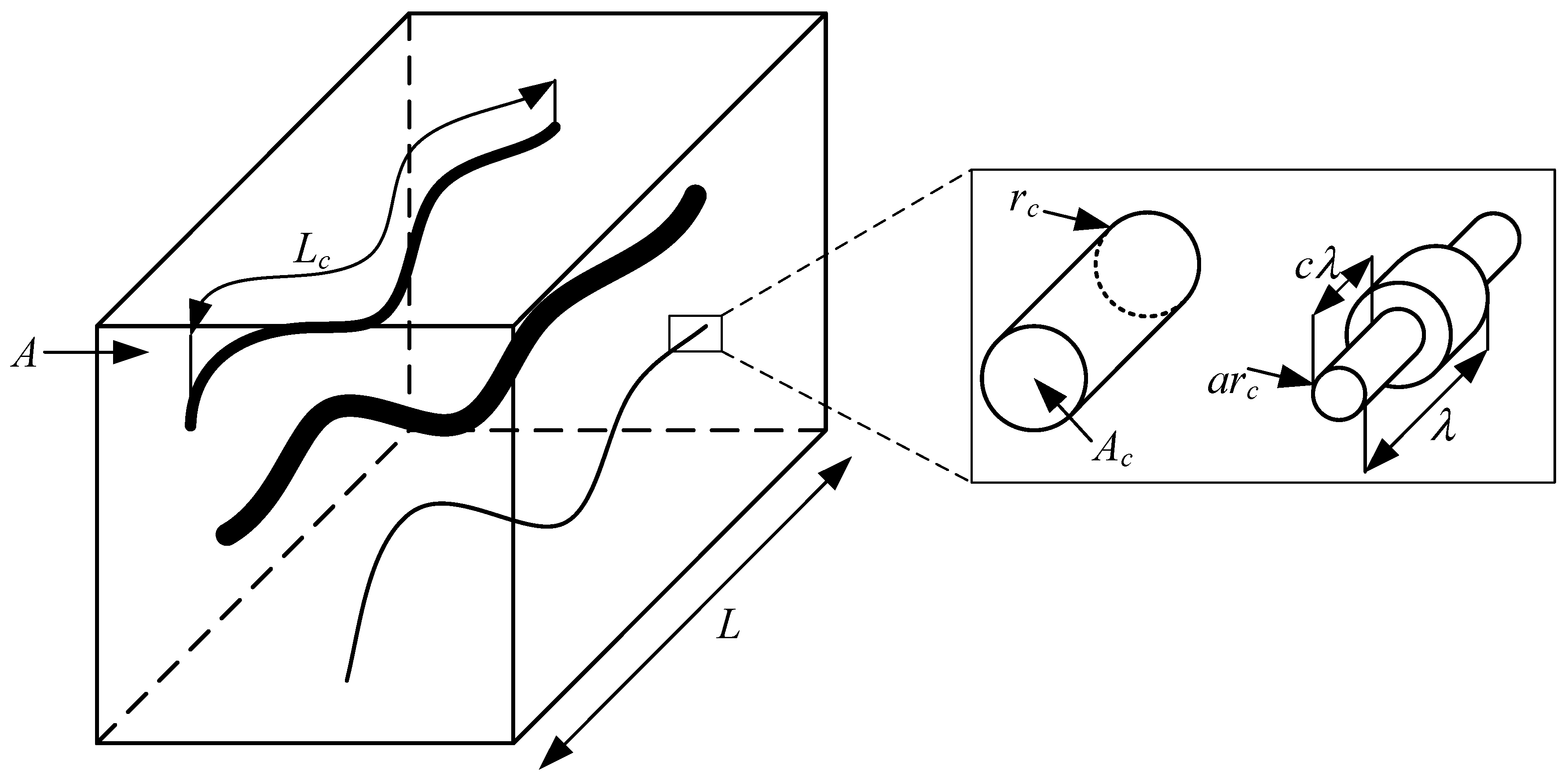
The classical BOCT model considers N capillaries, with each capillary permitted to have a different radius r_c. The capillaries are confined within a model of length L and area A, as displayed in Figure 1. Each capillary within the model is defined by a length L_c, tortuosity $t_c=L_c/L$ and a cross-sectional area to flow $A_c=\pi r_c$ [26,34].

The bundle of capillary tubes model deviates from the true pore structure of porous geologic media, as it is formulated on the assumption that there are no points of intersection between capillaries and that all capillaries run parallel with the same orientation [26]. It is widely acknowledged that the pore structure of geologic media is extremely complex, resulting in the effective porosity and absolute permeability of the media being highly dependent on the ratio of interconnected pore space [36]. However, for the simplicity of modelling, the assumption of zero intersections ensures that the transport of mass and electrical charge through the model takes place in only one direction [26]. Furthermore, in order to define an average tortuosity t for the model, it is assumed that the capillary radius r_c and length L_c are independent of each other.

The previously published works of Jackson [21,26] and Soldi et al. [37] define the distribution of capillary radii throughout the model differently. Jackson [21,26] states the number of capillaries with radius between $r_c$ and $r_c+d{r}_c$ as $n\left(r_c\right)d{r}_c$ such that the total number of capillary tubes is

$$N={{\displaystyle \int }}_{r_{min}}^{r_{max}}n(r_c)d{r}_c,$$

(1)

where N is the total number of capillaries, and $r_{min}$ and $r_{max}$ denote the minimum and maximum capillary radius within the model, respectively. The distribution of capillaries throughout the model is associated with the capillary radius by a function of the form [25].

$$n\left(r_c\right)\mathrm{d}{r}_c=D_J{\left(\frac{r_c-r_{max}}{r_{min}-r_{max}}\right)}^m,$$

(2)

where D_J is the normalization factor (constant, unitless) and 0 < m < ∞ (constant, unitless). The distribution function monotonically decreases at all values of m with the exception of m = 0, where the function produces a uniform distribution of capillary radii between $r_{min}$ and $r_{max}$ (Figure 3 in [26]). As the value of m increases, the frequency distribution is skewed more towards smaller radii values, similar to the skewed pore size distributions exhibited in many geologic porous media [26,38,39].

The frequency distribution of capillary radii presented by Soldi et al. [37] is somewhat different to that of Jackson [21,26]. Soldi et al. [37] assume that the number of pores with radii greater than or equal to a specific capillary radius R follows a fractal law such that [28,29,35,40]:

$$N\left(r_c\right)={\left(\frac{R_{REV}}{r_c}\right)}^{D_S}$$

(3)

where $0<r_{min}\le r_c\le r_{max}<R_{REV}$, D_S represents the dimensionless pore fractal dimension $\left(1<D_S<2\right)$ and R_REV is the radius of a cylindrical representative elementary volume (e.g., a cylindrical sample of porous geologic media) [37]. If $r_{max}=R_{REV}$, then $N=1$ and the cylindrical REV is entirely occupied by a single pore [35]. Conversely, if $r_{min}=0$, there are an infinite number of pores within the REV [35]. The cumulative pore size distribution (Equation (3)) is then differentiated with respect to $r_c$ to obtain an equivalent expression to Equation (2). The distribution of capillaries throughout the model is defined in terms of $dN\left(r_c\right)$, which represents the number of capillaries whose radii fall within the small range $r_c$ to $r_c+d{r}_c$ [37]:

$$dN\left(r_c\right)=D_S{R}_{REV}^D{r}_c{}^{-D_S-1}d{r}_c$$

(4)

A significant difference between the distributions produced from Equations (2) and (4) stems from a criterion of the model proposed by Soldi et al. [37] that the largest capillary must always exist. Unlike the frequency distribution of Jackson [21,26] (Equation (2)), that of Soldi et al. [37] (Equation (4)), cannot be skewed and so the accuracy of choice for r_max greatly influences how representative the BOCT model is of the modelled porous geologic media.

Nonetheless, by the implementation of capillary tubes with varying radii, the work of Soldi et al. [35,37] enhanced the BOCT model. The addition of pore throats within the model, rather than the constant radius approach adopted by Jackson [21,26], provides a more realistic representation of the pore structure in geologic media, thus enabling explicit modelling of residual phase saturation and impact of wettability alteration. The inset of Figure 1 displays the pore geometry of a single capillary tube proposed by Soldi et al. [35]. The radius at a particular point x along the length of a capillary is expressed as [35]:

$$r_c\left(x\right)=\{\begin{array}{c}a{r}_c \mathrm{if} x \in \left[0+\lambda n, c\lambda +\lambda n\right]\hfill \\ r_c \mathrm{if} x \in \left[c\lambda +\lambda n, \lambda +\lambda n\right]\hfill \end{array}$$

(5)

where a denotes the ratio in which the capillary radius is reduced, known as the radial factor ($0 \le a\le 1$, dimensionless), hence $a{r}_c$ represents the radius of the periodically distributed pore throats along the length of each capillary. It is assumed that each pore and its adjacent pore throat have a wavelength, or pattern length, $\lambda$, with the length of each capillary containing an integer number of wavelengths, $M$. Subsequently, the length of a pore throat is expressed as $c\lambda$, where $c$ represents the segment of $\lambda$ which contains a pore throat, also known as the length factor ($0 \le c\le 1$, dimensionless), and $n=0, 1, \dots M – 1$ [35].

Although the bundle of capillary tubes model is not the most accurate representation of the pore space in geologic media, the published works of Jackson [21,26] and Soldi et al. [37] individually provide good insight into the applications and advantages of modelling porous media as a bundle of tortuous capillary tubes. However, neither Jackson [21,26] nor Soldi et al. [37] considered non-monotonic capillary size distribution. On the other hand, Jougnot et al. [27] considered non-monotonic capillary size distribution but used the constant capillary radius approach, and their capillary size distribution was indirectly inferred from other modelled properties rather than from actually measured one. Moreover, many published studies investigated such non-monotonic pore size distribution and its effects on capillary pressure [41], relative permeability [42] or hydraulic conductivity [43]. However, to the best of the authors’ knowledge, such capillary distribution functions have never been used in modelling coupled electro-hydrodynamic problems. In this study, we present a new BOCT model that considers a non-monotonic pore size distribution based on experimentally measured pore size distribution and alternating capillary radius. Moreover, our new model is constructed to match the reported porosity and permeability values of a real sandstone sample and cross-compare the modelled hydro- and electrodynamic properties between the three types of capillary size distribution (termed Jackson, Soldi, New) and both constant and alternating capillary radius approaches. It should be noted that although our BOCT model was developed using available information on pore size distribution for a given rock sample, unlike in pore-network or direct pore-scale models, such information is not essential for BOCT models as capillary (pore) size distribution can be obtained from matching sample’s porosity and permeability.

2.2. Minimum and Maximum Capillary Radius

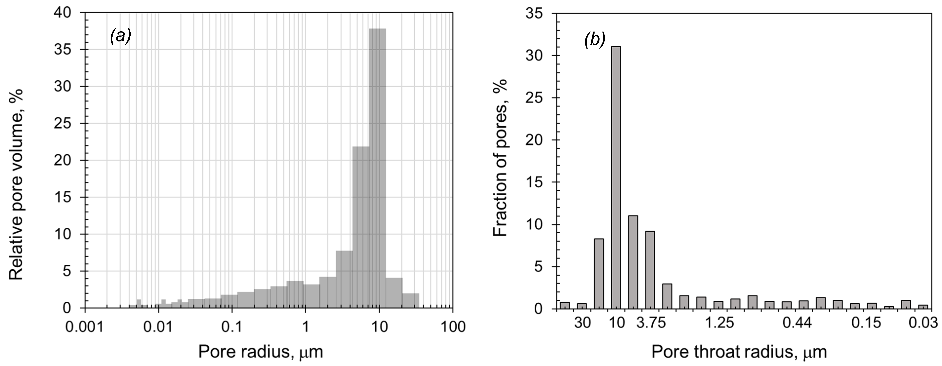
The Berea sandstone core sample, as discussed in Moore et al. [44], was modelled as a bundle of tortuous capillary tubes, assuming the system was water wet. Prior to implementing any capillary size distribution (CSD) function, a review of relevant literature surrounding Berea sandstone pore size distribution was conducted in order to determine the most appropriate minimum and maximum capillary radius to be used in the model.

Table 1. Pore and throat radii of Berea sandstone samples with respective porosity and absolute permeability. NMR is the Nuclear Magnetic Resonance.

Literature Reference	Method	Porosity (%)	Permeability (mD)	Pore Radius (μm)	Throat Radius (μm)
Hu et al. [45]	Micro-CT	10–25	500–5000	15	-
Li and Horne [38]	Mercury injection	23	804	10	-
Minagawa et al. [46]	NMR	-	-	14	14
Ott et al. [47]	Mercury injection	22	500	-	20
Thomson et al. [48]	Simulation (dry)	19.9	132–167	2.72	1.29
Thomson et al. [48]	Simulation (saturated)	15.8	61.5–115	2.72	1.32
Shi et al. [39]	Mercury injection	18.7	330	10	-

summarises the six key research papers consulted during the decision-making process, and Figure 2a,b present the pore size distributions from Shi et al. [39] and Li and Horne [38], respectively. The values of pore radius and throat radius given in Table 1 are either explicitly stated within the respective research paper as a single value or have been taken as the peak value from a pore size distribution curve.

The findings in the paper of Li and Horne [38] are presented in terms of pore throat diameter. Therefore, a rough assumption was made that the pore throat diameter was approximately equal to the pore radius, assuming a radial factor (ratio between throat and capillary radius) of 0.5, and so the pore radius has been reported as 5 μm in Table 1. Furthermore, Minagawa et al. [46] present a pore and throat size distribution as one figure, the peak of which sits at approximately 14 μm. Therefore, it has been assumed that this figure represents the average of all pore and throat radii, and so 14 μm has been presented in Table 1 as both the pore radius and the throat radius. The radius values from Ott et al. [47] and Thomson et al. [48] were determined to be outliers as they were, respectively, significantly larger and smaller than other values from the literature.

Initial values of r_min and r_max were considered by consulting the pore radius and throat data presented in Table 1 and Figure 2 and chosen to be 5 and 60 μm, respectively. The minimum value of 5 μm was selected due to the negligible pore volume of capillaries below this value, as depicted in Figure 2a, which will subsequently only be occupied by the wetting phase at the irreducible water saturation and will not contribute to flow within the core sample—therefore, having no impact on the permeability of the model. The minimum r_max value considered was 60 μm, again selected based on the maximum radius presented in Figure 2a. However, the simulation procedure was conducted using r_max of both 60 μm and 100 μm to investigate the influence of r_max on the distribution functions.

2.3. Matching Porosity and Permeability to Berea Sandstone

The porosity and permeability of the BOCT model were calculated using Jackson (2010) (Equations (4) and (5), respectively). Three CSD functions were then investigated, with their constants and exponents adjusted accordingly, in order to match the porosity of the model to the porosity of the Berea sandstone sample reported as 18.75% in Moore et al. [44]. Since no permeability was provided by Moore et al. [44], the permeability of the Berea core sample, and therefore BOCT model, was estimated from the literature data obtained from experimental procedures (Table 1). This resulted in a permeability range of 10s to low 100s mD being considered acceptable for a sample with 18.75% porosity.

Accurately predicting the tortuosity of the Berea sample was key in matching all three CSD functions, as tortuosity is required to calculate both porosity and absolute permeability using both Jackson and New approaches (note the porosity and permeability calculation using New CSD relies on Jackson [21] Equations (4) and (5)). To compute the sample porosity using the Soldi CSD also requires tortuosity (Equation (5) in [37]). The tortuosity of the model was calculated using studies of Civan (2007, Equations (3)–(14)) and Jougnot et al. ([15], Equation 4.29), in which F represents the formation factor of the Berea sandstone, which was explicitly stated as 24 in Moore et al. [44]. The Civan [49] and Jougnot et al. [15] approaches yielded tortuosity of 4.33 and 2.12, respectively. An additional calculation method outlined by Tiab and Donaldson [50] returned a tortuosity of 10.77, whilst Zecca et al. [51] recorded tortuosities of 4.3 and 4.5 for Berea sandstone using water and methane at 3 MPa, respectively. Attia et al. [52] measured tortuosities in the range of 3.78–4.71 for Berea sandstone, with an average value of 4.16. Therefore, range of values was investigated to determine the most realistic tortuosity and value of 4.5 was selected for a sample with porosity of 18.75%. In this study, we assumed the tortuosity to be independent of phase saturation, consistent with published studies [53,54].

2.4. Constant Capillary Radius

The first CSD examined was that proposed by Jackson [26] using Equation (2) and constant capillary radius. When manipulating the m and D_J parameters of the Jackson CSD, it was imperative to decide on whether the total number of capillaries was kept constant or the total volume of capillaries was constant. As $r_{min}$ and $r_{max}$ were predetermined based on literature values, in order to accurately replicate the sample examined by Moore et al. [44] for which the absolute permeability was not reported, the values of m and D_J were optimised until the porosity of the BOCT model matched that of the Berea core sample (18.5%), therefore ensuring the total volume of capillaries remained constant. Furthermore, it was crucial to ensure that the CSD resembled the pore size distributions depicted in Figure 2a (the right-hand side at pore radii greater than 6 μm) whilst still ensuring a realistic permeability for the model consistent with literature values (Table 1). It was, therefore, important to first choose the exponent m that gave the general shape of the distribution required and then to adjust D_J to achieve a porosity of 18.75%.

The second capillary size distribution examined was Soldi CSD using Equation (4). As all values of $r_c$ had already been incrementally distributed between $r_{min}$ and $r_{max}$ and R_REV was a fixed value of 12,500 μm taken from Moore et al. [44], the only parameter which could be adjusted to match the desired porosity was the fractal dimension, D_S. Therefore, the fractal dimension was manipulated until the porosity of the BOCT model matched that of the Berea sandstone sample.

Following the review of the literature surrounding Berea pore size distribution, the findings of Shi et al. [39] were determined to be the most similar to the core plug examined by Moore et al. [44]. This conclusion was drawn as the porosity reported in both papers was the same, and the permeability reported by Shi et al. [39] fell nicely within the range of permeability expected of Berea sandstone. Furthermore, Shi et al. [39] presented a detailed pore size distribution as displayed in Figure 2a, and for these reasons, the New CSD for the BOCT model was predominantly based on these findings.

The desired shape of the New CSD was replicated by modifying Jackson [26] distribution (Equation (2)) and invoking three intervals such that to capture the peak pore radius observed in the literature:

$$\left(r_c\right)\mathrm{d}{r}_c=\{\begin{array}{ccc}{D}_1{\left(\frac{r_c-r_{min}}{r_{max}-r_{min}}\right)}^{m_1}\hfill & for& r_{min}\le r_c \le 10 \mathrm{\mu }\mathrm{m}\\ constant& for& 10 \mathrm{\mu }\mathrm{m}<r_c<12 \mathrm{\mu }\mathrm{m}\\ D_2{\left(\frac{r_c-r_{max}}{r_{min}-r_{max}}\right)}^{m_2}\hfill & for& 12 \mathrm{\mu }\mathrm{m}\le r_c \le r_{max}\end{array}$$

(6)

The limits of each interval were determined by calculating the average pore size from the data in Table 1, which resulted in an average peak pore radius of 11 μm, thus informing on the location and the width of the peak. As before, $D_1$ and $D_2$ represent the normalisation factors of the first and third interval, respectively, with m₁ and m₂ being the respective skewing constants.

Table 2. Values required for each parameter of Soldi, Jackson and New CSD functions to obtain porosity of 18.75% for constant radius BOCT model when $d{r}_c=0.1$ μm. Number of significant figures varies due to the requirement to match porosity exactly.

Distribution	Parameter	rmax = 60 μm	rmax = 100 μm
Soldi	DS	1.31875	1.2565
Jackson	DJ	1185.32	342.74
	m	10	10
New	D1	39,850	119,990
	m1	2	2
	D2	978.4	1131
	m2	8	16

displays the final values required for the parameters of all three distribution functions for the BOCT model with constant capillary radius, each resulting in a porosity of 18.75%. Bearing in mind the typically expected permeability of Berea sandstone from literature (Table 1), it was concluded that the values in Table 2 resulted in the most accurate and realistic pore size distributions and permeabilities for the model with 18.75% porosity, with

Table 3. Permeability and number of capillaries within the model for Soldi, Jackson and New CSD functions with constant capillary radius and a model porosity of 18.75% when $d{r}_c=0.1 \mathsf{\mu }\mathrm{m}$.

Distribution	rmax = 60 μm		rmax = 100 μm
	Permeability (mD)	No. Capillaries	Permeability (mD)	No. Capillaries
Soldi	1313	29,532	3562	18,404
Jackson	263	59,861	686	29,772
New	409	29,638	434	29,393

providing the resulting permeability and total number of capillaries within the model.

It is clear that the permeability obtained with Soldi CSD using Equation (4) is outside the expected range of the literature. This is caused by the inability to skew the Soldi CSD function towards smaller capillaries due to the criterion of the model that the largest capillary must always exist.

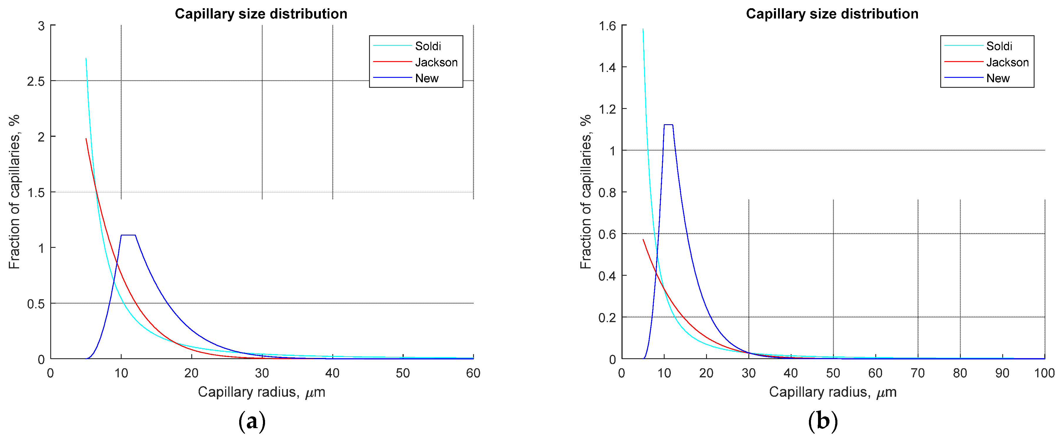
Figure 3 presents a comparison of each distribution function using Equations (2), (4) and (6) with a maximum capillary radius of 60 μm (Figure 3a) and 100 μm (Figure 3b). It can be seen from Figure 3 and Table 3 that the New CSD provides a more realistic size distribution as it is non-monotonic, as expected from real rocks, and it results in significantly fewer capillaries with radius less than 10 μm compared with Soldi and Jackson CSD. Both the Soldi and Jackson CSD require a large number of small capillaries to accommodate for the porosity of 18.75%, while these capillaries do not contribute significantly to flow and hence the permeability. Moreover, increasing r_max to 100 μm results in nearly 3-fold increase in the model permeability using the Soldi and Jackson CSD functions, while the permeability obtained with the New distribution remains fairly constant, which is consistent with real rock permeability behaviour if very few larger pores are added to (found in) the sample.

2.5. Alternating Capillary Radius

To model the CSD with alternating capillary radius requires determination of the radial (a) and length (c) factors in Equation (5). Examining micro-CT images and pore network modelling, such as the work of Sharqaway [55], allowed average a and c values to be estimated. Furthermore, the published work of Shehata et al. [56] determined the pore throat radius of Berea to be in the range of 2.5–25 μm, therefore permitting minimum and maximum radial factors of approximately 0.5 and 0.85, respectively. Upon sensitivity analysis of the a and c (not presented here) and consultation of Sharqaway [55] and Shehata et al. [56], a radial factor $a=0.7$ and length factor $c=0.2$ were decided to be the most representative of Berea sandstone whilst returning desired permeability values.

Equations for porosity and permeability of the model were altered to account for the implementation of pore throats. The porosity of the model was calculated using an altered form of Equation (4) from Jackson [21] such that:

$$\varphi =\frac{\pi t}{A}\underset{r_{min}}{\overset{r_{max}}{{\displaystyle \int }}}{f}_v\left(a,c\right) r_c^2 n\left(r_c\right)d{r}_c$$

(7)

where t is the previously defined tortuosity of the model, A is the cross-sectional area of the Berea sandstone sample and $f_v \left(a,c\right)$ is a dimensionless volume factor (same as Equation (6) in Soldi et al., [37]):

$$f_v\left(a,c\right)=c\left(a^2-1\right)+1$$

(8)

Similarly, the permeability of the model was calculated using an altered form of Equation (5) from Jackson [21] such that:

$$k=\frac{\varphi }{8t^2}\frac{{\int }_{r_{min}}^{r_{max}}{f}_k\left(a,c\right) r_c^4 n\left(r_c\right)d{r}_c }{{\int }_{r_{min}}^{r_{max}}{f}_v\left(a,c\right) r_c^2 n\left(r_c\right)d{r}_c}$$

(9)

where $f_k\left(a,c\right)$ is a permeability factor that quantifies the reduction in volumetric flow rate due to the pore throats (same as Equation (18) in [37]):

$$f_k\left(a,c\right)=\frac{a^4}{c+a^4\left(1-c\right)}$$

(10)

Implementing the radial and length factors into Equations (8) and (10) resulted in volume and permeability factors, f_v and f_k, of 0.898 and 0.612, respectively.

Table 4. Values required for each parameter of Soldi, Jackson and New distribution functions to obtain porosity of 18.75% with alternating radius water wet bundle of capillary tubes model with radial and length factors of 0.7 and 0.2, respectively, when $d{r}_c=0.1 \mathsf{\mu }\mathrm{m}$. Number of significant figures varies due to the requirement to match porosity exactly.

Distribution	Parameter	rmax = 60 μm	rmax = 100 μm
Soldi	DS	1.3341	1.27275
Jackson	DJ	1319.82	381.57
	m	10	10
New	D1	44,350	133,650
	m1	2	2
	D2	1089.2	1259.3
	m2	8	16

displays the final values required for the parameters of all three distribution functions—Equations (2), (4) and (6)—for BOCT model with alternating capillary radius, each resulting in a porosity of 18.75%, with capillary radii distributed in increments ($d{r}_c$) of 0.1.

The permeability and total number of capillaries within the bundle of capillary tubes model using each of the distribution functions is detailed in

Table 5. Permeability and number of capillaries within the model for Soldi, Jackson and New distribution functions with alternating capillary radius and model porosity of 18.75% with radial and length factors of 0.7 and 0.2, respectively, when $d{r}_c=0.1 \mathsf{\mu }\mathrm{m}$.

Distribution	rmax = 60 μm		rmax = 100 μm
	Permeability (mD)	No. Capillaries	Permeability (mD)	No. Capillaries
Soldi	227	33,355	615	20,926
Jackson	46	66,653	120	33,145
New	71	32,991	76	32,733

. The addition of pore throats resulted in a permeability reduction of approximately 83% with all distribution functions. Since the porosity of the model was reduced by the volume factor, the number of capillaries within each model also increased to achieve the desired porosity of 18.75% by 11.3% for both the Jackson and New distribution functions, and 12.9% and 13.7% for the Soldi distribution model with r_max of 60 μm and 100 μm, respectively.

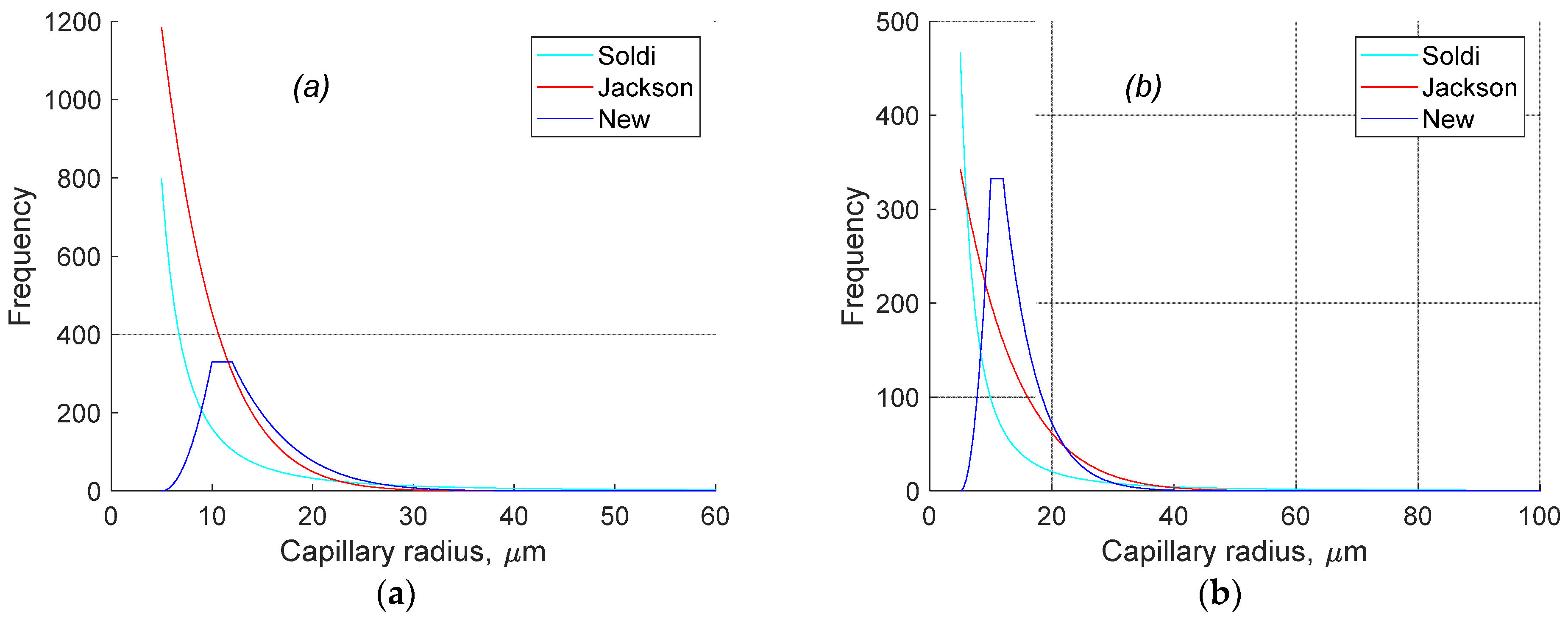
The shape of the capillary size distribution curves remained the same as before with the constant capillary radius model for all three distribution functions, i.e., the m, m₁ and m₂ exponents required for the Jackson and New distribution functions were untouched. The only aspect of the CSD that changed was the number of capillaries of each size (y-axis magnitude), as apparent in Figure 4. The change is due to the reduced volume of each capillary and thus the need for a greater number of capillaries within the model to achieve a porosity of 18.75%.

2.6. Multi-Phase Flow Simulation

The model was then extended to multi-phase flow by considering a wetting phase w (water) and an immiscible non-wetting phase nw (CO₂ as in [44]). Based on experimental data [57], Berea sandstones exhibit strongly water-wet behaviour when saturated with liquid CO₂ and high salinity brine. In the experiments conducted by Moore et al. [44] Berea sample was also saturated with liquid CO₂, but tap water was used. Considering the thermodynamics of wettability [58], it is expected that water wetness should increase with decreasing salinity. Therefore, we assumed that our BOCT model is strongly water-wet, and we only consider this case. Moreover, an assumption was made that capillaries occupied by the non-wetting CO₂ contain a thin immobile layer of water [21]. This volumetrically insignificant layer of water was included in the model as it contributes to the surface electrical conductivity ${\sigma }_{sw}$ and regulates the development of an electrical double layer in the wetting phase (e.g., [59]). It was also assumed that the non-wetting CO₂ is non-conductive, and therefore there is no electrical double layer in the non-wetting phase and associated with its surface electrical conductivity.

To determine water saturation, S_w, and the relative permeability to wetting phase, k_rw, of the model with constant capillary radius, we used the approach described by Jackson ([21]; Equations (6) and (7), respectively).

The relative streaming potential coupling coefficient C_r was calculated as a function of water saturation using both Equations (31) and (33) from Jackson [21], assuming a thin and thick electrical double layer, respectively. In order to adopt the thick double-layer assumption for the model, the surface conductivity must dominate—i.e., the two electrical double layers at opposite sides of the capillary must overlap, resulting in bulk conductivity of the wetting water, ${\sigma }_w$, being negligible compared with ${\sigma }_{sw}$. A criterion was therefore implemented to ensure that the correct C_r assumption was used within the model, such that if ${\sigma }_{sw}$ is less than 10% of ${\sigma }_w$, then the thin double-layer assumption was used; otherwise, the thick double-layer assumption was used.

Equations for water saturation, relative streaming potential coupling coefficient and relative electrical conductivity of the model were altered to account for the implementation of pore throats using the approach outlined by Soldi et al. [37]. Note that Rembert et al. [32] proposed a similar approach (pore and throats) using a different pattern and a fractal capillary size distribution to describe the electrical conductivity in saturated conditions. We introduced two new factors to quantify the reduction in capillary radius due to the presence of pore throats ($0\le f_r\left(a,c\right)\le 1$), and the reduction in $r_c^3$ ($0\le f_{cc}\left(a,c\right)\le 1$):

$$f_r\left(a,c\right)={{\displaystyle \int }}_0^{\lambda }r\left(x\right) dx=\left[{{\displaystyle \int }}_0^{\lambda c}\left(ra\right) dx+{{\displaystyle \int }}_{\lambda c}^{\lambda } r dx\right]=c\left(a-1\right)+1$$

(11)

$$f_{cc}\left(a,c\right)={{\displaystyle \int }}_0^{\lambda }{r}^3\left(x\right) dx=\left[{{\displaystyle \int }}_0^{\lambda c}{\left(ra\right)}^3 dx+{{\displaystyle \int }}_{\lambda c}^{\lambda } r^3 dx\right]=c\left(a^3-1\right)+1$$

(12)

For the alternating capillary radius model, the corresponding equations for the relative electrical conductivity and the relative streaming potential coupling coefficient invoking the thin and thick double-layer assumptions become:

$${\sigma }_r\left(S_w\right)=\frac{{\sigma }_w{\int }_{r_{min}}^{r_{w max}}{f}_v\left(a,c\right) r_c^2 n\left(r_c\right)d{r}_c + 2{\sigma }_{sw}{\int }_{r_{min}}^{r_{max}} f_r\left(a,c\right) r_c n\left(r_c\right)d{r}_c}{{\sigma }_w{\int }_{r_{min}}^{r_{max}}{f}_v\left(a,c\right) r_c^2 n\left(r_c\right)d{r}_c + 2{\sigma }_{sw}{\int }_{r_{min}}^{r_{max}} f_r\left(a,c\right) r_c n\left(r_c\right)d{r}_c}$$

(13)

$$C_r\left(S_w\right)=\frac{\left[\frac{{\int }_{r_{nw min}}^{r_{w max}} f_v\left(a,c\right) r_c^2 n\left(r_c\right)d{r}_c}{{\int }_{r_{nw min}}^{r_{max}} f_v\left(a,c\right) r_c^2 n\left(r_c\right)d{r}_c}\right]}{{\sigma }_r\left(S_w\right)}$$

(14)

$$C_r\left(S_w\right)=\frac{\left[\frac{{\int }_{r_{nw min}}^{r_{w max}} f_{cc}\left(a,c\right) r_c^3 n\left(r_c\right)d{r}_c}{{\int }_{r_{nw min}}^{r_{max}} f_{cc}\left(a,c\right) r_c^3 n\left(r_c\right)d{r}_c}\right]}{{\sigma }_r\left(S_w\right)}$$

(15)

In Equations (13)–(15) $r_{w max}$ refers to the radius of the largest capillary occupied by the wetting water, and a minimum radius of capillaries that could be occupied by the nonwetting CO₂ is referred to as $r_{nw min}$. To investigate an impact on hydroelectrodynamic properties, multiple values of the irreducible water saturation, S_wirr, were used, ranging from 0 to 0.5 using different values of $r_{nw min}$.

3. Results and Discussion

3.1. Relative Permeability to Water

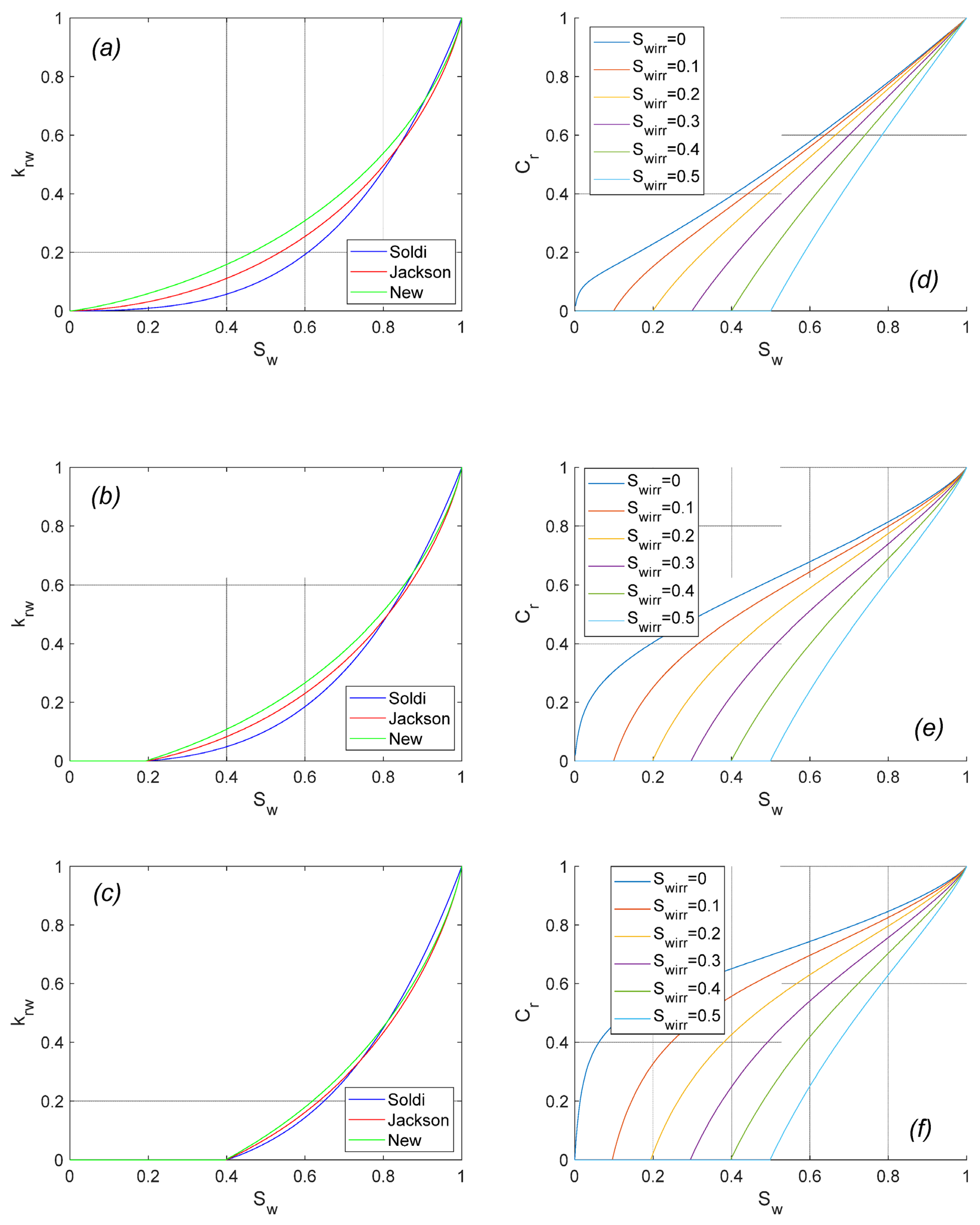
The relative permeability to water at S_wirr between 0 and 0.4 for all three distribution functions investigated are displayed in Figure 5a–c for the models of alternating radius capillaries, when $r_{max}=100 \mathsf{\mu }\mathrm{m}$. Implementing the code for capillaries of varying aperture into the bundle of capillary tubes model had a negligible effect on the relative permeability results compared with the constant radius results when plotted as a function of water saturation (e.g., [37]), and therefore the latter are not presented. We explain this observation by the fashion in which the pore throats are modelled using the radial and length factors, which results in a reduction of the average capillary radii while not explicitly capturing the residual trapping of the non-wetting CO₂, hence allowing the entire capillary to be occupied by either wetting or non-wetting phase. In reality, in some capillary tubes, depending on the capillary entry pressure, only pores (and usually not pore throats) should be occupied by the non-wetting phase via the so-called snap-off mechanism, which would have an impact on the relative permeability.

However, it is clear from Figure 5 that the distribution of capillary radii throughout the model has a significant impact on the gradient of the k_rw curve at low irreducible water saturations, with each distribution producing notably different values of k_rw in the domain $k_{rw}\le 0.8$ when $S_{wirr}=0$. The model constructed using the New distribution function has larger relative permeabilities at lower water saturation, whilst the relative permeability of the Soldi model increases notably slower. As S_wirr increases towards 0.4, the k_rw curves of each of the three distribution functions gradually move closer together and begin to overlap. These results suggest that the distribution of capillary radii throughout the BOCT model becomes less significant to the relative permeability of the model as the irreducible water saturation increases.

3.2. Relative Streaming Potential Coupling Coefficient

The relative streaming potential coupling coefficient C_r was investigated for all three distribution functions invoking both the thin and thick double-layer assumptions. It was found that alternating capillary radius did not have any noticeable effect on C_r for either CSD or whether the thin or thick double-layer assumption was invoked. This is explained by the inability of the current model to capture realistic residual trapping of the non-wetting phase, thus assuming that any capillary tube in its entirety is occupied either by water or by CO₂ regardless of whether the corresponding capillary has a constant or alternating radius. Moreover, varying the capillary size distribution function had no noticeable effect on C_r when employing the limit of a thin double layer. This conclusion was drawn when considering both zero and non-zero (${\sigma }_{sw}$ is less than 10% of ${\sigma }_w$) surface conductivities.

Moore et al. [44] used tap water of 125 $\Omega ·\mathrm{m}$ electrical resistivity in their streaming potential measurements. Another experimental study on multi-phase streaming potential measurements [18] reported values of C_r as a function of S_w using liquid non-polar undecane and 0.01 mol/L NaCl solution of approximately 10 $\Omega ·\mathrm{m}$ resistivity. Consistent with previously reported results [60], surface conductivity becomes dominant when the bulk resistivity exceeds 10 $\Omega ·\mathrm{m}$. Therefore, we apply the thick double-layer assumption to describe the water saturation dependence of C_r and compare the modelling results to the published experimental data. Figure 5d–f displays the relative coupling coefficient results for all three capillary size distribution functions investigated, assuming a thick electrical double layer, with model $r_{max}=100 \mathsf{\mu }\mathrm{m}$ and capillaries of alternating radius at various S_wirr values from 0 to 0.5. We do not present results obtained with constant capillary radii as they are essentially identical to those with alternating radii. The difference between the three capillary size distribution functions became apparent when analysing the C_r results considering a thick electrical double layer—particularly at small values of S_wirr (between 0 and 0.2). The New distribution function presents the sharpest decrease in C_r as S_wirr approaches 0 in comparison with other CSD functions, which mimics the results reported by Vinogradov and Jackson ([18]; Figure 3a,c) and simulated by Zhang et al. ([22]; Figure 13a,c). The results presented in Figure 5 demonstrate that more accurate modelling of the capillary size distribution is capable of capturing the experimentally observed behaviour of the C_r(S_w). However, the C_r behaviour with S_w obtained using the Jackson CSD closely resembles the results of the New CSD. On the other hand, the Soldi CSD does not provide as steep of decrease in C_r at proximity to 0 of S_w, thus suggesting this approach is least suitable for simulating the electrokinetic properties of the type of rocks studied here due to the very large number of small capillaries in the fractal distribution.

3.3. Bundle of Capillary Tubes vs. Experimental Results of Moore et al. (2004)

In order to simulate C_r of the Berea sandstone sample, the surface conductivity ${\sigma }_{sw}$ was determined to match the reported water electrical conductivity and that of the fully water-saturated rock sample of 3.03 × 10⁻³ S/m [44].

To determine the surface conductivity ${\sigma }_{sw}$ of the Berea sample, MATLAB (MathWorks, Natick, MA, USA) scripts were written to calculate the effective conductivity and conductance of a single capillary, the total conductance of all capillaries within the model constructed using each of the three distribution functions, and finally, the conductivity of the water-saturated sample:

$${\sigma }_{rw}=\left[{{\displaystyle \int }}_{r_{min}}^{r_{max}}\left({\sigma }_w+\frac{2{\sigma }_{sw}}{r_c f_r\left(a,c\right)}\right)\frac{\pi r_c^2{f}_v\left(a,c\right)}{tL}\right]\left(\frac{L}{A}\right)$$

(16)

where L and A are the length and area of the Berea sandstone sample, respectively. The results for each distribution function and r_max values are displayed in

Table 6. Surface conductivity of the model for Soldi, Jackson and New distribution functions with capillaries of alternating radius and model porosity of 18.75% required to match the conductivity of the water-saturated rock measured by Moore et al. [43]. Number of significant figures varies due to the requirement to match conductivity exactly.

Distribution	$\mathbf{Surface} \mathbf{Conductivity}, {\mathit{\sigma }}_{\mathit{s}\mathit{w}} \left(\mathbf{S}\right)$
	rmax = 60 μm	rmax = 100 μm
Soldi	2.8305 × 10−6	3.9592 × 10−6
Jackson	1.7221 × 10−6	2.5662 × 10−6
New	2.3668 × 10−6	2.38515 × 10−6

. As the surface conductivity is multiplied by the number of capillaries with a radius between $r_c$ and $r_c+d{r}_c$, the distribution of capillary radii throughout the model is therefore a limiting factor of the surface conductivity and, as such, each distribution at each value of r_max resulted in different surface conductivities. Comparing the results of Table 6 with those of Table 5, it is suggested that the surface conductivity correlates with the permeability of the model in some way, as the surface conductivity increases with increased permeability. This makes sense as the decrease of permeability is due to an increasing number of small capillaries, hence an increase of specific surface area and therefore more surface with an electrical double layer generating this surface conductivity. Due to the formulation of the New distribution function and subsequent similarity in model permeability independent of the r_max value selected, the New distribution was the only distribution that resulted in similar surface conductivities for r_max of 60 μm and 100 μm. As the bulk conductivity of tap water within the pore space of the Berea sample was measured to be 8 × 10⁻³ S/m (8 × 10⁻⁹ S/μm) by Moore et al. [44], the bundle of capillary tubes model is dominated by the surface conductivity since it is three orders of magnitude larger than the bulk conductivity in capillaries of an order of 1 μm and one order of magnitude larger than the bulk conductivity in the largest tested capillary tubes of 100 μm (note that the bulk conductivity is multiplied by the $r_c^2$ term and the surface conductivity is multiplied by the $r_c$ term in Equation (16)). The high surface conductivities presented in Table 6 are indeed expected as the bulk electrolyte (tap water) salinity is at least 1 order of magnitude lower than the threshold salinity at which the surface conductivity becomes dominant in sandstones [60] and comparable to the corresponding value for sand packs [61].

The streaming potential coupling coefficient of the fully water-saturated rock sample was calculated with respect to the zeta potential using:

$$C\left(S_w=1\right)=\frac{\frac{{\epsilon }_w {\zeta }_w}{{\mu }_w} {\int }_{r_{min}}^{r_{max}} f_v\left(a,c\right) r_c^2 n\left(r_c\right)d{r}_c}{{\sigma }_w {\int }_{r_{min}}^{r_{max}} f_v\left(a,c\right) r_c^2 n\left(r_c\right)d{r}_c+2{\sigma }_{sw}{\int }_{r_{min}}^{r_{max}} f_r\left(a,c\right) r_c n\left(r_c\right)d{r}_c}$$

(17)

Invoking thin double layer and assuming the electric permittivity and viscosity of water to be $7.1\times {10}^{-10}\mathrm{F}/\mathrm{m}$ and $8.9\times {10}^{-4}\mathrm{Pa}·\mathrm{s}$, respectively, with the aim of achieving the coupling coefficient of −300 mV/MPa as reported by Moore et al. [44]. Although Jackson [21] and Linde [62] derived expressions to compute $C\left(S_w=1\right)$ in the limit of a thick double layer, the proposed equations use the surface charge density, which is neither reported nor can be interpreted from Moore et al. [44], and for that reason, we used Equation (17). The bulk conductivity of the model was set to the measured value of the core sample (8 × 10⁻³ S/m), and the zeta potential ζ was assumed to be −28 mV as calculated by Moore et al. [44]. The coupling coefficient at $S_w=1$ was calculated for each distribution function with r_max values of 60 μm and 100 μm using the respective surface conductivities ${\sigma }_{sw}$ determined previously.

Unsurprisingly, the simulated coupling coefficient for the fully water-saturated rock sample under each of the distribution functions does not match the coupling coefficient of −300 mV/MPa reported by Moore et al. [44]—the simulated coupling coefficient is −62 mV/MPa, which is approximately five times smaller. However, in order to simulate liquid CO₂ flooding of a tap-water-saturated sample and to match the relative coupling coefficient of the model to that of Moore et al. [44], it is not necessary to match $C\left(S_w=1\right)$ of the model to that of Moore et al. [44].

The relative streaming potential coupling coefficient of the BOCT model was simulated under the thick double-layer assumption using Equation (15), with the aim of replicating the relative coupling coefficient of 0.1 reported by Moore et al. [44]. The simulated relative coupling coefficient results are presented in

Table 7. Actual irreducible water saturation of the Berea sample for various reported irreducible water saturations when $C_r\left(S_{wirr}\right)=0.1$, assuming the presence of a thick electrical double layer. Actual irreducible water saturations determined for Soldi, Jackson and New distribution functions with capillaries of alternating radius and model porosity of 18.75%, when $r_{max}=100 \mathsf{\mu }\mathrm{m}$.

Reported Swirr	Actual Irreducible Water Saturation When ${\mathit{C}}_{\mathit{r}}\left({\mathit{S}}_{\mathit{w}\mathit{i}\mathit{r}\mathit{r}}\right)=0.1$
	Soldi CSD	Jackson CSD	New CSD
0.2	0.15	0.17	0.18
0.3	0.25	0.26	0.27
0.4	0.35	0.35	0.36
0.5	0.46	0.46	0.46

for models with $r_{max}=100 \mathsf{\mu }\mathrm{m}$, and which summarises the actual S_wirr of the Berea sample for a range of possible values which could be reported by Moore et al. [44]. Based on the S_wirr values reported in the literature for Berea sandstone, C_r was initially simulated for S_wirr in the range 0.2–0.5. Since according to our model, a non-zero coupling can only occur when water is flowing within the Berea sample, acknowledging that if water is still flowing, then the irreducible water saturation has not yet been reached. This is consistent with the conclusions drawn by Vinogradov and Jackson [18] and Zhang et al. [22]. On the other hand, an experimental study published by Allègre et al. [63] reported a non-zero streaming potential coupling coefficient at irreducible water saturation and presented an empirical model to explain this behaviour. However, the model heavily relied on an abnormal relative streaming potential coupling coefficient of an order of 30 at partial water saturation. To the best of our knowledge, such large values of C_r have not been reported by any other research group, hence the empirical parameter introduced by Allègre et al. [63] that allowed C_r at partial saturation to be 200 greater than the corresponding value at S_w = 1 was considered to be irrelevant for our model describing experimental conditions when $C_r\left(S_{wirr}\right)\ll 1$.

The results in Table 7 are designed to be analysed such that if Moore et al. [44] report $C_r \left(S_{wirr}=0.32\right)=0.1$, the true S_wirr should be 0.21, 0.22 and 0.22 for the Soldi, Jackson and New CSD functions, respectively. Therefore, Table 7 effectively demonstrates the magnitude of the error within S_wirr of Moore et al. [44], with the largest and the smallest discrepancies between the reported and actual S_wirr being established with the Soldi and New distribution functions, respectively. However, at the reported S_wirr of 0.3 and above, the actual S_wirr of all distributions is approximately the same.

Following the comparison of the BOCT model results and experimental results of Moore et al. [44], this work confirms that the Moore et al. [44] paper must be corrected for the actual S_wirr, since it is not possible to achieve a non-zero coupling coefficient at the irreducible water saturation due to the lack of a flowing electrolyte. Our model also suggests that a more accurate New CSD function should be used in BOCT models to capture the behaviour of C_r with water saturation. Moreover, it is suggested to explicitly implement the residual trapping of a non-wetting phase in the BOCT model with alternating capillary radius.

4. Conclusions

The bundle of capillary tubes model developed in this study to simulate the streaming potential coupling coefficient in partially saturated porous media is based on a realistic pore and pore throat size distribution of real rock samples. Compared with previously published studies, our model produces results that are more consistent with existing experimental data.

• Unlike the previous bundle of parallel capillaries models, our approach to defining the pore and pore throat radii distribution is based on direct measurements, thus providing a more realistic description of porous rocks, in which pore and pore throat size distribution is non-monotonic;
• Our model was tested using constant and alternating capillary radii, with the latter being invoked in order to distinguish between pores and pore throats. Despite the alternating capillary radii model’s capability, we did not attempt to explicitly model residual trapping of the non-wetting phase in this work. Hence, we found no noticeable difference in the relative permeability and the relative streaming potential coupling coefficient modelled using either straight or variable radii capillary tubes;
• Our model produces considerably different relative permeability curves with small irreducible water saturation (<0.2) in comparison with previously published studies of Jackson [21] and Soldi et al. [37]. However, there is no noticeable difference between modelled curves using either of the approaches if irreducible water saturation is larger than 0.2;
• Compared with the results published by Jackson [21] and Soldi et al. [37], the relative streaming potential coupling coefficient simulated with our model appears to be more stable at high water saturation and to decrease more rapidly to zero as water saturation approaches the irreducible value. This behaviour is consistent with published experimental results, thus suggesting that the non-monotonic capillary size distribution should be used for more accurate characterisation of multi-phase flow in porous media;
• Our model was used to simulate measurements of the streaming potential coupling coefficient in sandstone samples saturated with aqueous solution and liquid CO₂ [44]. The model assumed a thick double layer approach for computing the coupling coefficient, consistent with the use of tap water in the experiments. The modelling results suggest that true irreducible water saturation was not reached in the experiments reported by Moore et al. [44]. This conclusion is consistent with the hypothesis that explained a non-zero coupling coefficient in the experiments of Vinogradov and Jackson [18]. Moreover, since our model produces qualitatively more accurate behaviour of the coupling coefficient with decreasing water saturation, the discrepancy between the reported by Moore et al. [44] irreducible water saturation and the modelled true value was the smallest with our approach relative to that of Jackson [21] or Soldi et al. [37];
• To improve the quality of the here-developed bundle of capillary tubes model requires explicit representation of the residual (capillary) trapping of the non-wetting phase. This modification will be developed in a future study using the alternating capillary radii and will potentially allow a more accurate depiction of hysteretic behaviour of the streaming potential coupling coefficient during saturation and desaturation of the modelled rock with the non-wetting phase;
• Due to its simplicity, the here-reported and to-be-improved bundle of capillary tubes model can be used to accurately simulate the evolution of the streaming potential coupling coefficient during multi-phase flow in porous media, thus providing an efficient means for a variety of geophysical applications.

References

- WWAP United Nations World Water Assessment Programme. United Nations World Water Development Report 2014; UNESCO: Paris, France, 2014. [Google Scholar]
- Barlow, P.M.; Reichard, E.G. Saltwater intrusion in coastal regions of North America. Hydrogeol. J. 2010, 18, 247–260. [Google Scholar] [CrossRef]
- Binley, A.; Hubbard, S.S.; Huisman, J.A.; Revil, A.; Robinson, D.A.; Singha, K.; Slater, L.D. The emergence of hydrogeophysics for improved understanding of subsurface processes over multiple scales. Water Resour. Res. 2015, 51, 3837–3866. [Google Scholar] [CrossRef] [PubMed] [Green Version]
- Jouniaux, L.; Maineult, A.; Naudet, V.; Pessel, M.; Sailhac, P. Review of self-potential methods in hydrogeophysics. Comptes Rendus Geosci. 2009, 341, 928–936. [Google Scholar] [CrossRef] [Green Version]
- Revil, A.; Jardani, A. The Self-Potential Method: Theory and Applications in Environmental Geosciences; Cambridge University Press: Cambridge, UK, 2013. [Google Scholar]
- MacAllister, D.J.; Jackson, M.D.; Butler, A.P.; Vinogradov, J. Remote detection of saline intrusion in a coastal aquifer using borehole measurements of self-potential. Water Resour. Res. 2018, 54, 1669–1687. [Google Scholar] [CrossRef] [Green Version]
- Jougnot, D.; Linde, N.; Haarder, E.B.; Looms, M.C. Monitoring of saline tracer movement with vertically distributed self-potential measurements at the HOBE agricultural site, Voulund, Denmark. J. Hydrol. 2015, 521, 314–327. [Google Scholar] [CrossRef] [Green Version]
- Voytek, E.; Barnard, H.; Jougnot, D.; Singha, K. Transpiration- and precipitation-induced subsurface water flow observed using the self-potential method. Hydrol. Process. 2019, 33, 1784–1801. [Google Scholar] [CrossRef] [Green Version]
- Roubinet, D.; Linde, N.; Jougnot, D.; Irving, J. Streaming potential modeling in fractured rocks: Insight into identification of hydraulically-active fractures. Geophys. Res. Lett. 2016, 43. [Google Scholar] [CrossRef] [Green Version]
- Hu, K.; Jougnot, D.; Huang, Q.; Looms, M.C.; Linde, N. Advancing quantitative understanding of self-potential signatures in the critical zone through long-term monitoring. J. Hydrol. 2020, 585, 124771. [Google Scholar] [CrossRef] [Green Version]
- Linde, N.; Doetsch, J.; Jougnot, D.; Genoni, O.; Duerst, Y.; Minsley, B.J.; Luster, J. Self-potential investigations of a gravel bar in a restored river corridor. Hydrol. Earth Syst. Sci. 2011, 15, 729–742. [Google Scholar] [CrossRef] [Green Version]
- Jackson, M.D.; Gulamali, M.Y.; Leinov, E.; Saunders, J.H.; Vinogradov, J. Spontaneous potentials in hydrocarbon reservoirs during waterflooding: Application to water-front monitoring. SPE J. 2012, 17, 53–69. [Google Scholar] [CrossRef]
- Leinov, E.; Jackson, M.D. Experimental measurements of the SP response to concentration and temperature gradients in sandstones with application to subsurface geophysical monitoring. J. Geophys. Res. Solid Earth 2014, 119, 6855–6876. [Google Scholar] [CrossRef] [Green Version]
- Hunter, R.J. Zeta Potential in Colloid Science; Academic: New York, NY, USA, 1981. [Google Scholar]
- Jougnot, D.; Roubinet, D.; Guarracino, L.; Maineult, A. Modeling streaming potential in porous and fractured media, description and benefits of the effective excess charge density approach. In Advances in Modeling and Interpretation in Near Surface Geophysics; Springer: Cham, Switzerland, 2020; pp. 61–96. [Google Scholar]
- Graham, M.; Macallister, D.; Vinogradov, J.; Jackson, M.; Butler, A. Self-potential as a predictor of seawater intrusion in coastal groundwater boreholes. Water Resour. Res. 2018, 54, 6055–6071. [Google Scholar] [CrossRef] [Green Version]
- Vinogradov, J.; Jackson, M.D.; Chamerois, M. Zeta potential in sandpacks: Effect of temperature, electrolyte pH, ionic strength and divalent cations. Colloids Surf. Physicochem. Eng. Asp. 2018, 553, 259–271. [Google Scholar] [CrossRef]
- Vinogradov, J.; Jackson, M.D. Multiphase streaming potential in sandstones saturated with gas/brine and oil/brine during drainage and imbibition. Geophys. Res. Lett. 2011, 38, L01301. [Google Scholar] [CrossRef]
- Guichet, X.; Jouniaux, L.; Pozzi, J.P. Streaming potential of a sand column in partial saturation conditions. J. Geophys. Res. Solid Earth 2003, 108, B3. [Google Scholar] [CrossRef]
- Revil, A.; Cerepi, A. Streaming potentials in two-phase flow conditions. Geophys. Res. Lett. 2004, 31, L11605. [Google Scholar] [CrossRef]
- Jackson, M.D. Multiphase electrokinetic coupling: Insights into the impact of fluid and charge distribution at the pore scale from a bundle of capillary tubes model. J. Geophys. Res. 2010, 115, B07206. [Google Scholar] [CrossRef]
- Zhang, J.; Vinogradov, J.; Leinov, E.; Jackson, M.D. Streaming potential during drainage and imbibition. J. Geophys. Res. Solid Earth 2017, 122, 4413–4435. [Google Scholar] [CrossRef]
- Blunt, M.J.; Bijeljic, B.; Dong, H.; Gharbi, O.; Iglauer, S.; Mostaghimi, P.; Paluszny, A.; Pentland, C. Pore-scale imaging and modelling. Adv. Water Resour. 2013, 51, 197–216. [Google Scholar] [CrossRef] [Green Version]
- Jougnot, D.; Mendieta, A.; Leroy, P.; Maineult, A. Exploring the effect of the pore size distribution on the streaming potential generation in saturated porous media, insight from pore network simulations. J. Geophys. Res. Solid Earth 2019, 124, 5315–5335. [Google Scholar] [CrossRef]
- Hao, L.; Cheng, P. Pore-scale simulations on relative permeabilities of porous media by lattice Boltzmann method. Int. J. Heat Mass Transfer. 2010, 53, 1908–1913. [Google Scholar] [CrossRef]
- Jackson, M.D. Characterization of multiphase electrokinetic coupling using a bundle of capillary tubes model. J. Geophys. Res. 2008, 113, B04201. [Google Scholar] [CrossRef] [Green Version]
- Jougnot, D.; Linde, N.; Revil, A. Doussan CDerivation of soil-specific streaming potential electrical parameters from hydrodynamic characteristics of partially saturated soils. Vadose Zone J. 2012, 11, 1–15. [Google Scholar] [CrossRef] [Green Version]
- Tyler, S.W.; Wheatcraft, S.W. Fractal processes in soil water retention. Water Resour. Res. 1990, 26, 1047–1054. [Google Scholar] [CrossRef]
- Yu, B.; Li, J.; Li, Z.; Zou, M. Permeabilities of unsaturated fractal porous media. Int. J. Multiph. Flow 2003, 29, 1625–1642. [Google Scholar] [CrossRef]
- Guarracino, L. Estimation of saturated hydraulic conductivity Ks from the van Genuchten shape parameter α. Water Resour. Res. 2007, 43, W11502. [Google Scholar] [CrossRef]
- Pfannkuch, H.O. On the correlation of electrical conductivity properties of porous systems with viscous flow transport coefficients. In Developments in Soil Science; Elsevier: Amsterdam, The Netherlands, 1972; Volume 2, pp. 42–54. [Google Scholar] [CrossRef]
- Rembert, F.; Jougnot, D.; Guarracino, L. A fractal model for the electrical conductivity of water-saturated porous media during mineral precipitation-dissolution processes. Adv. Water Resour. 2020, 145, 103742. [Google Scholar] [CrossRef]
- Chu, Z.; Zhou, G.; Li, R. Enhanced fractal capillary bundle model for effective thermal conductivity of composite-porous geomaterials. Int. Commun. Heat Mass Transf. 2020, 113, 104527. [Google Scholar] [CrossRef]
- Dullien, F.A.L. Porous Media: Fluid Transport and Pore Structure, 2nd ed.; Academic Press: San Diego, CA, USA, 1992; p. 574. [Google Scholar]
- Soldi, M.; Guarracino, L.; Jougnot, D. A Simple Hysteretic Constitutive Model for Unsaturated Flow. Transport. Porous Media 2017, 120, 271–285. [Google Scholar] [CrossRef] [Green Version]
- Abou-Kassem, J.H.; Farouq Ali, S.M.; Rafiq Islam, M. Chapter 2—Single-Phase Fluid Flow Equations in Multidimensional Domain. In Petroleum Reservoir Simulations; Gulf Publishing Company: Huoston, TX, USA, 2006; pp. 7–41. [Google Scholar]
- Soldi, M.; Guarracino, L.; Jougnot, D. An effective excess charge model to describe hysteresis effects on streaming potential. J. Hydrol. 2020, 588, 124949. [Google Scholar] [CrossRef]
- Li, K.; Horne, R.N. Experimental Study and Fractal Analysis of Heterogeneity in Naturally Fractured Rocks. Fractal Characterization of the geysers rock. Transp. Porous Med. 2009, 78, 217–231. [Google Scholar] [CrossRef]
- Shi, J.Q.; Xue, Z.; Durucan, S. Supercritical CO2 core flooding and imbibition in Berea sandstone—CT imaging and numerical simulation. Energy Procedia 2011, 4, 5001–5008. [Google Scholar] [CrossRef] [Green Version]
- Soldi, M.; Jougnot, D.; Guarracino, L. An analytical effective excess charge density model to predict the streaming potential generated by unsaturated flow. Geophys. J. Int. 2019, 216, 380–394. [Google Scholar] [CrossRef] [Green Version]
- Kosugi, K. Three-parameter lognormal distribution model for soil water retention. Water Resour. Res. 1994, 30, 891–901. [Google Scholar] [CrossRef]
- Kosugi, K. Lognormal distribution model for unsaturated soil hydraulic properties. Water Resour. Res. 1996, 32, 2697–2703. [Google Scholar] [CrossRef]
- Malama, B.; Kuhlman, K.L. Unsaturated hydraulic conductivity models based on truncated lognormal pore-size distributions. Ground Water 2015, 53, 498–502. [Google Scholar] [CrossRef] [Green Version]
- Moore, J.R.; Glaser, S.D.; Morrison, F.H. The streaming potential of liquid carbon dioxide in Berea sandstone. Geophys. Res. Lett. 2004, 31. [Google Scholar] [CrossRef] [Green Version]
- Hu, D.; Wyatt, D.; Chen, C.; Martysevich, V. Correlating Recovery Efficiency to Pore Throat Characteristics Using Digital Rock Analysis. In SPE Digital Energy Conference and Exhibition; Society of Petroleum Engineers: Texas, TX, USA, 2015. [Google Scholar]
- Minagawa, H.; Nishikawa, Y.; Ikeda, I.; Miyazaki, K. Characterization of sand sediment by pore size distribution and permeability using proton nuclear magnetic resonance measurement. J. Geophys. Res. Atmos. 2008, 113. [Google Scholar] [CrossRef]
- Ott, H.; Andrew, M.; Snippe, J.; Blunt, M.J. Microscale solute transport and precipitation in complex rock during drying. Geophys. Res. Lett. 2014, 41, 8369–8376. [Google Scholar] [CrossRef] [Green Version]
- Thomson, P.-R.; Aituar-Zhakupova, A.; Hier-Majumder, S. Image Segmentation and Analysis of Pore Network Geometry in Two Natural Sandstones. Front. Earth Sci. 2018, 6, 58. [Google Scholar] [CrossRef] [Green Version]
- Civan, F. Petrographic Characteristics of Petroleum-Bearing Formations. Reserv. Form. Damage 2007. [Google Scholar] [CrossRef]
- Tiab, D.; Donaldson, E.C. Formation Resistivity and Water Saturation. In Petrophysics (Fourth Edition): Theory and Practice of Measuring Reservoir Rock and Fluid Transport; Elsevier: Amsterdam, The Netherlands, 2016; pp. 187–278. [Google Scholar]
- Zecca, M.; Honari, A.; Vogt, S.J.; Bijeljic, B.; May, E.F.; Johns, M.L. Measurements of Rock Core Dispersivity and Tortuosity for Multi-Phase Systems. In International Symposium of the Society of Core Analysts; Snowmass: Colorado, CO, USA, 2016. [Google Scholar]
- Attia, A.M.; Fratta, D.; Bassiouni, Z. Irreducible Water Saturation from Capillary Pressure and Electrical Resistivity Measurements. Oil Gas. Sci. Technol. 2008, 63, 203–217. [Google Scholar] [CrossRef] [Green Version]
- Clennell, M.B. Tortuosity: A guide through the maze. Geol. Soc. Lond. Spec. Publ. 1997, 122, 299–344. [Google Scholar] [CrossRef]
- Ghanbarian, B.; Hunt, A.G.; Ewing, R.P.; Sahimi, M. Tortuosity in porous media: A critical review. Soil Sci. Soc. Am. J. 2013, 77, 1461–1477. [Google Scholar] [CrossRef]
- Sharqaway, M.H. Construction of pore network models for Berea and Fontainebleau sandstones using non-linear programing and optimization techniques. Adv. Water Resour. 2016, 98, 198–210. [Google Scholar] [CrossRef]
- Shehata, A.M.; Kumar, H.; Nasr-El-Din, H.A. New Insights on Relative Permeability and Initial Water Saturation Effects during Low-Salinity Waterflooding for Sandstone Reservoirs. In Proceedings of the SPE Trinidad and Tobago Section Energy Resources Conference, Port of Spain, Trinidad and Tobago, 13–15 June 2016. Society of Petroleum Engineers. [Google Scholar]
- Haeri, F.; Tapriyal, D.; Sanguinito, S.; Fuchs, S.J.; Shi, F.; Dalton, L.E.; Baltrus, J.; Howard, B.; Matranga, C.; Crandal, D.; et al. CO2-brine contact angle measurements on Navajo, Nugget, Bentheimer, Bandra Brown, Berea, and Mt. Simon Sandstones. Energy Fuels 2020, 34, 6085–6100. [Google Scholar] [CrossRef]
- Hirasaki, G.J. Wettability: Fundamentals and Surface Forces. SPE Form. Eval. 1991, 6, 217–226. [Google Scholar] [CrossRef]
- Revil, A.; Pezard, P.A.; Glover, P.W.J. Streaming potential in porous media 1. Theory of the zeta potential. J. Geophys. Res. Solid Earth 1999, 104, 20021–20031. [Google Scholar] [CrossRef]
- Vinogradov, J.; Jaafar, M.Z.; Jackson, M.D. Measurement of streaming potential coupling coefficient in sandstones saturated with natural and artificial brines at high salinity. J. Geophys. Res. 2010, 115, B12204. [Google Scholar] [CrossRef] [Green Version]
- Lorne, B.; Perrier, F.; Avouac, J.-P. Streaming potential measurements: 1. Properties of the electrical double layer from crushed rock samples. J. Geophys. Res. 1999, 104, 17857–17877. [Google Scholar] [CrossRef] [Green Version]
- Linde, N. Comment on “Characterization of multiphase electrokinetic coupling using a bundle of capillary tubes model”. J. Geophys. Res. 2009, 114, B06209. [Google Scholar] [CrossRef] [Green Version]
- Allègre, V.; Jouniaux, L.; Lehmann, F.; Sailhac, P. Streaming potential dependence on water-content in Fontainebleau sand. Geophys. J. Int. 2010, 182, 1248–1266. [Google Scholar] [CrossRef] [Green Version]
Figure 1.
The bundle of capillary tubes (bold curves) model. The inset to the right shows the two representations of modelled capillaries having the (i) constant (left) and (ii) alternating (right) radius. In the alternating capillary radius model, the pore throat is modelled by a reduced radius , while the pore throat length is defined by , where is the pattern length, which is described in more detail below [35].
Figure 2.
Pore size distribution of Berea sandstone reported in terms of (a) pore radius, extracted from Shi et al. [39], and (b) pore throat radius, extracted from Li and Horne [38].
Figure 3.
Frequency distribution comparison of Soldi, Jackson and New CSD functions using straight capillaries with tortuosity of 4.5, , and (a) and (b) .
Figure 4.
Comparison of Soldi, Jackson and New distribution functions using alternating capillaries with tortuosity of 4.5, , and (a) and (b) with radial and length factors of 0.7 and 0.2, respectively.
Figure 5.
Relative permeability (a–c) and relative streaming potential coupling coefficient (d–f) of the BOCT model constructed using the Soldi (a,d), Jackson (b,e) and New (c,f) distribution functions with capillaries of alternating radius assuming a thick electrical double layer and significant surface conductivity with maximum capillary radius of 100 μm.